| Issue |
A&A
Volume 691, November 2024
|
|
|---|---|---|
| Article Number | A27 | |
| Number of page(s) | 10 | |
| Section | Extragalactic astronomy | |
| DOI | https://doi.org/10.1051/0004-6361/202449892 | |
| Published online | 28 October 2024 | |
X-ray observations of Blueberry galaxies
1
Astronomical Institute of the Czech Academy of Sciences, Boční II 1401, CZ-14100 Prague, Czech Republic
2
Physics Department, & Institute of Theoretical and Computational Physics, University of Crete, GR 71003 Heraklion, Greece
3
Institute of Astrophysics, Foundation for Research and Technology-Hellas, GR 71110 Heraklion, Greece
4
Cahill Center for Astronomy and Astrophysics, California Institute of Technology, Pasadena, CA 91125, USA
5
FZU – Institute of Physics of the Czech Academy of Sciences, Na Slovance 1999/2, Prague 182 21, Czech Republic
6
LERMA, Observatoire de Paris, CNRS, PSL Univ., Sorbonne Univ., 75014 Paris, France
7
Collège de France, 11 Place Marcelin Berthelot, 75005 Paris, France
8
Univ. Grenoble Alpes, CNRS, IPAG, 38000 Grenoble, France
⋆ Corresponding author; barbora.adamcova@asu.cas.cz
Received:
7
March
2024
Accepted:
9
August
2024
Context. Compact star-forming galaxies were dominant galaxy types in the early Universe. Blueberry galaxies (BBs) represent their local analogues, being very compact and having intense star formation.
Aims. Motivated by high X-ray emission recently found in other analogical dwarf galaxies, called Green Peas, we probed the X-ray properties of BBs to determine if their X-ray emission is consistent with the empirical laws for star-forming galaxies.
Methods. We performed the first X-ray observations of a small sample of BBs with the XMM-Newton satellite. Spectral analysis for detected sources and upper limits measured via Bayesian-based analysis for very low-count measurements were used to determine the X-ray properties of our galaxy sample.
Results. Clear detection was obtained for only two sources, with one source exhibiting an enhanced X-ray luminosity to the scaling relations. For the remaining five sources, only an upper limit was constrained, suggesting BBs to be rather underluminous as a whole. Our analysis shows that the large scatter cannot be easily explained by the stochasticity effects. While the bright source is above (and inconsistent with) the expected distribution at almost the 99% confidence level, the upper limits of the two sources are below the expected distribution.
Conclusions. These results indicate that the empirical relations between the star formation rate, metallicity, and X-ray luminosity might not hold for BBs with uniquely high specific star formation rates. One possible explanation could be that the BBs may not be old enough to have a significant X-ray binary population. The high luminosity of the only bright source can then be caused by an additional X-ray source, such as a hidden active galactic nucleus or more extreme ultraluminous X-ray sources.
Key words: galaxies: dwarf / galaxies: star formation
© The Authors 2024
 Open Access article, published by EDP Sciences, under the terms of the Creative Commons Attribution License (https://creativecommons.org/licenses/by/4.0), which permits unrestricted use, distribution, and reproduction in any medium, provided the original work is properly cited.
This article is published in open access under the Subscribe to Open model. Subscribe to A&A to support open access publication.
1. Introduction
Compact star-forming galaxies allow us to study various astrophysical processes, from star formation in extreme environments to the broader context of galaxy evolution and cosmic history. Low-mass, low-metallicity compact dwarf galaxies were abundant at the early stages of the Universe. The intense star formation ignited in such compact dwarf galaxies is proposed, along with the high-energy emission from first quasars, to be responsible for the reionisation of the Universe (see, e.g. Robertson et al. 2010). The main mechanism responsible for the epoch of reionisation, which took place after the Dark Ages in the early Universe (corresponding to the cosmological redshift z ∼ 30 − 6), is still hotly debated. The recently launched James Webb Space Telescope (JWST) enables the direct study of these high-redshift galaxies (see recent studies by Harikane et al. 2023; Finkelstein et al. 2023). However, a detailed study of these distant primordial galaxies is challenging due to the limited sensitivity of observations across wavelengths. Therefore, the local galaxies with properties analogous to those of the early-Universe galaxies represent unique environments for multi-wavelength studies.
One of the local analogues of the high-redshift galaxies includes the Green Pea galaxies (GPs), z ∼ 0.2 − 0.3, compact (≤5 kpc), low-mass (∼109 M⊙), and low-metallicity (log(O/H) + 12 ∼ 8.1) starburst galaxies with high star formation rates (SFR ∼ 10 − 100 M⊙ yr−1), originally identified in a citizen-science Galaxy Zoo project of classification of the optical Sloan Digital Sky Survey (SDSS) observations (Cardamone et al. 2009). The characteristic green colour is due to a strong emission from ionised oxygen heated by the presence of recently formed stars. Similar to high-redshift galaxies, GPs are also strong Lyα emitters (Henry et al. 2015; Verhamme et al. 2017; Orlitová et al. 2018), and the escape of a significant amount of ionising ultraviolet (UV) radiation (also called the Lyman continuum) has been observed in some of them (Izotov et al. 2016, 2018a,b). Most recently, Schaerer et al. (2022), Rhoads et al. (2023) revealed a high level of similarity between the JWST spectra of high-redshift galaxies and GPs.
Somewhat surprising results came from X-ray observations of GPs with the X-ray Multi-Mirror Mission (XMM-Newton). Unusually bright X-ray emission was detected in two out of three of the sources (Svoboda et al. 2019), and the reported X-ray luminosities, ∼1042 erg s−1, were a factor of > 5 larger than predicted from any theoretical or empirical relation established for star-forming galaxies (e.g. Ranalli et al. 2003; Brorby et al. 2016). The enhancement of the X-ray emission of the two GPs is too strong to be due to stochasticity, the enhanced population of high-mass X-ray binaries (HMXBs), or ultraluminous X-ray sources (ULXs). It was also shown that the contribution from hot gas cannot explain the high X-ray luminosity (Franeck et al. 2022). One of the feasible remaining explanations is the presence of an active galactic nucleus (AGN), where the X-ray emission originates in the accretion processes onto a massive black hole (Svoboda et al. 2019). In dwarf galaxies, such massive black holes would represent a lower end of the mass range for super-massive black holes or might be considered as intermediate-mass black holes, with masses around ∼104 − 105 M⊙ (see studies by Mezcua et al. 2016, 2018).
The GPs are, by definition, at redshift z ≳ 0.2 − 0.3. Yang et al. (2017) identified a sample of local GP analogues using selection criteria similar to those for the GPs (compactness, large equivalent width of optical emission lines), but limited to z < 0.1 SDSS galaxies. Due to their lower redshift, the characteristic colour of these galaxies is blue, and therefore they were called ‘Blueberry galaxies’ (BBs). Similarly, McKinney et al. (2019) and Jaskot et al. (2019) focused their sample on galaxies with the highest ionisation (high [O III]/[O II] line ratio), as analogues to Lyman continuum leakers. As a shorthand, we refer to both these samples as BBs. Compared to GPs, the BBs typically have lower metallicities (log(O/H) + 12 ∼ 7.6−8.1) and lower stellar masses (M* < 108 M⊙). The specific star formation rate (sSFR), defined as the star formation rate per unit of stellar mass (SFR/M⋆), is higher (logsSFR > −8) than for GPs. Thus, BBs not only represent good analogues to the high-redshift galaxies, but also significantly extend the parameter space at which scaling relations between star formation properties and X-ray luminosity can be studied.
This paper contains the first study of X-ray emission of a sample of BBs observed with the XMM-Newton satellite. The paper is structured as follows: first we discuss the observation sample and provide details of the data reduction and analysis in Section 2, then present our results in Section 3, and discuss them in Section 4.
2. Observation sample, data reduction, and analysis
We defined the parent sample of the BBs by combining the two samples mentioned above: (1) Yang et al. (2017) – 40 sources and (2) Jaskot et al. (2019) – 13 sources. For all of the galaxies in the combined parent sample, we calculated the expected X-ray luminosity using the Brorby et al. (2016) scaling relation. The parent sample of BBs includes SFR values estimated under the assumption of the Kroupa (2001) initial mass function (IMF); therefore, we had to modify the Brorby et al. (2016) relation, which was constrained assuming the Salpeter (1955) IMF. Throughout this paper, we adopt the values based on the Kroupa (2001) IMF. To use the Brorby et al. (2016) scaling relation or to compare with different galaxy samples, we used the conversion described by Madau & Dickinson (2014) (i.e. to convert the SFR from Salpeter 1955 IMF to Kroupa 2001 IMF, we multiplied by a constant factor of 0.67).
After using the adjusted Brorby et al. (2016) relation, we selected eight galaxies for X-ray observations based on their expected X-ray fluxes, choosing those with the shortest exposure time needed for their detection in X-rays. Given that the X-ray emission of star-forming galaxies is mainly correlated with the SFR (Grimm et al. 2003; Lehmer et al. 2010), and that the flux naturally drops with the distance, the selected sources are those with the largest SFRs and the lowest redshift from the parent sample. Table 1 lists the full names, coordinates, and main physical properties of the selected sources. Our targets lie in the redshift range z = 0.03 − 0.09, their SFRs are ∼0.5 − 10 M⊙ yr−1 (based on Hα measurements from Yang et al. 2017; Jaskot et al. 2019), their stellar masses log M⋆ = 7.2 − 8.7 M⊙ (obtained from the ugrizy photometry for the Yang et al. 2017 sample and from the MPA-JHU catalogue for the Jaskot et al. 2019 sample), and their metallicities log[O/H] + 12 ∼ 7.6−8.1 (measured here using the prescription of Pettini & Pagel 2004).
Sample of BBs with the expected highest X-ray flux from the parent sample.
Our selected sources, except BB6, were observed by the XMM-Newton satellite from January to April 2021 with the use of the EPIC cameras operating in full-frame mode with a thin filter (for observation details, see Table 2). BB6 was not observed; therefore, it is excluded from the subsequent data reduction and analysis. The total exposure times of the seven observed BBs ranged from 17 to 61 ks per source, but after the subtraction of intervals with high background flares (see below), the net exposure times shrank significantly in some cases (see Table 2 for the clean exposure times for each camera). The most strongly affected source was BB5, for which the useful exposure shrank from 25 to 5 ks in the pn camera (to 10 and 9 ks in MOS1 and MOS2 cameras, respectively), which meant that only a small fraction (less than 25%) of the observing time could be used.
Observation details and results of the XSPEC and BEHR analysis.
For the data reduction, we used version 20.0.0 of the Science Analysis System software (SAS; Gabriel et al. 2004). First, the SAS commands epproc and emproc were used to obtain the calibrated and concatenated event lists for the pn and MOS detectors, which were subsequently filtered using the tabgtigen and evselect tools in order not to contain intervals of high particle background. The count rate threshold of 0.4 ct s−1 and energy range of 10 < E < 12 keV were assumed for pn, and the count rate threshold of 0.35 ct s−1 and E > 10 keV were assumed for MOS.
The SAS script EDETECT_CHAIN was used to perform the detection of weak sources in several energy bands (namely 0.5 − 10, 0.5 − 1, 1 − 2, 2 − 4.5, and 4.5 − 10 keV) at the same time. The detection criteria were based on the emldetect tool with a minimum detection likelihood of eight. If a source was detected by this script, we followed with the spectra extraction. For a particular observation, the source and background regions were determined identically for the pn and MOS cameras. The counts from these regions were then extracted using the evselect tool. The spectra of the point-like sources were extracted as circular regions around the source coordinates from SDSS with a standard radius of 30 arcsec. To define the background regions, we used the recommendation for the pn and MOS cameras given in the XMM-Newton Calibration Technical Note XMM-SOC-CAL-TN-0018 (Smith & Guainazzi 2022). First, the background and source regions cannot overlap, as out-of-time events are to be avoided. As is recommended for the pn camera, the background regions were chosen to have comparable low-energy instrumental noise to the source region– that is, on the same chip of the CCD detector and with a similar distance from the readout node. As the MOS detectors have a less severe limitation (only the same chip is required), we used the same background regions as for the pn and only visually checked for any contamination by bright sources in the background regions (for the background region coordinates, see Table A.1).
As the combination of spectra from the EPIC cameras is possible only if the spectra are generated with a common bin size, a common bin size of 5 eV was chosen for all EPIC cameras. For the pn detector, only patterns less than four and the standard energy range of 0 − 20479 eV were considered; for the MOS detector, less than 12 and a range of 0 − 11999 eV. For the extracted spectra, the redistribution matrices were generated using the rmfgen task, and the ancillary files using the arfgen. This allowed for the combination of the spectra into the EPIC combined spectrum via the epicspeccombine tool. For the detected sources, we used the combined spectra for the spectral analysis. For different energy bands (namely 0.5 − 1, 1 − 2, and 2 − 10 keV), the EPIC vignetting-corrected background-subtracted images1 were created for our sources.
We analysed the X-ray spectra of the X-ray-detected sources with the XSPEC spectral fitting software (v12.12, Arnaud 1996), using the energy range of 0.5 − 10 keV. When a background model is not included in the spectral fitting, XSPEC uses W-statistics (Wachter et al. 1979), which are also referred to as modified C-statistics2 For the fitting, the combined EPIC spectra were binned using the ftgrouppha tool to contain at least one count in a single bin, which is recommended for the XSPEC implementation of the W-statistics. An absorbed power-law model, phabs*powerlaw, was used for the spectral model, Iν ≈ ν−α with frequency ν, and spectral slope α. The abundances were set to values from Anders & Grevesse (1989), and the (Verner et al. 1996) photo-ionisation cross-sections were used. In X-ray astronomy, the photon index (Γ, where Γ = α + 1) is used to describe the power-law slope and is associated with the X-ray emission produced by typical X-ray binary (XRB) populations. For the XSPEC analysis, Γ and the normalisation factor were left to vary, and the uncertainties on the fitted parameters were calculated using the err command in the 90% confidence ranges for each parameter. The hydrogen column density, NH, was set to values calculated from the galaxy coordinates via the nH calculator3, since we assume the absorption to be only the neutral absorption in our Galaxy. The fluxes and luminosities were then determined using the flux and lum commands in XSPEC.
For the rest of the sources, which were undetected by the SAS detection script due to low count rates, Bayesian analysis in low count regimes had to be applied, mainly because we cannot directly subtract the background from the source spectra. We used the Bayesian Estimation of Hardness Ratios (BEHR4) code (Park et al. 2006) to determine the posterior probability distribution of the counts in each of the undetected sources.
The same process of defining the source and background regions as for the detected sources was applied (see above). We used the SAOImage DS9 (Joye & Mandel 2003) region statistics tool on the images (energy range being 0.5−10 keV) and measured the number of counts and the area of the previously defined regions. As no prior information about the sources was known, we used the non-informative Jeffrey’s prior distribution (Φ = 1/2). The X-ray flux for each source was determined via the use of the WebPIMMS5 tool. To convert the count rate posteriors to fluxes, a power-law model was used. The photon index was assumed to be Γ = 1.9, as that is the usual value for star-forming galaxies (see Basu-Zych et al. 2013). The X-ray luminosity was then calculated as LX = 4πDL2FX, where DL is the luminosity distance and FX is the X-ray flux measured in 0.5 − 8 keV. The Λ cold dark matter model is assumed throughout this work: Hubble constant H0 = (67.4 ± 0.5) km s−1 Mpc−1 and matter density parameter Ωm = 0.315 (Planck Collaboration VI 2020).
Parameters and results of the XSPEC fitting.
3. Results
The measured X-ray fluxes and derived X-ray luminosities for detected sources (using XSPEC), as well as the measured upper limits for the undetected ones (determined using the BEHR code and a 68% confidence interval for the upper limits), are summarised in Table 2. The last column lists the predicted values of X-ray luminosities from the Brorby et al. (2016) relation. Only two sources, BB1 and BB8, have a significant detection revealed by the aforementioned SAS detection script. They both have the X-ray luminosity log LX ≳ 40.4 erg s−1, but the X-ray luminosity for BB8 is about five times larger than the expected one from the SFR and metallicity. Both sources are detected in the softest X-ray bands (0.5−1 and 1−2 keV), but only BB8 is also detected in the harder 2−10 keV band. The results of the XSPEC spectral analysis using the absorbed power-law model are given in Table 3. We obtained good fits for both BBs, with the Γ ≈ 1.9 for BB1 and Γ ≈ 1.7 for BB8. The X-ray spectra of our two BBs are shown in Fig. 2, along with their best-fit power-law models and their residuals. We also tested an APEC spectral model, but we did not obtain any better fit.
For the two detected sources, we created the X-ray vignetting-corrected background-subtracted images for three energy bands, 0.5–1 keV, 1–2 keV, and 2–10 keV, and we obtained the optical images from the SDSS DR16 SkyServer6 (Fig. 1). BB1 has a strong detection in the 0.5–1 and 1–2 keV bands, while BB8 also shows a significant detection in the harder 2–10 keV band. The optical images reveal that BB1 has extended features, whereas BB8 appears to be very compact. Additionally, there is a source near BB1 which is classified as a star in the SDSS DR16 SkyServer and therefore does not contribute to the X-ray energy band.
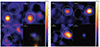 |
Fig. 1. X-ray vignetting-corrected background-subtracted images for BB1 (left) and BB8 (right) in the three used energy bands, 0.5–1 keV, 1–2 keV, and 2–10 keV (from top left to bottom left), and the SDSS optical images (bottom right). The source extraction regions (solid white open circles) and background regions (dot-dashed white open circles) are denoted in the figures (see the appendix for details of the extraction regions). The dashed green open rectangles, present in each X-ray image, indicate the regions corresponding to the SDSS images. The X-ray images are given in linear scale using the minima and maxima of the image cutouts. The colour scale denotes the pixel intensity, i.e. the scaled and weighted count rate per pixel. The SDSS images are shown at a different size scale than the X-ray images since a larger field of view would not provide adequate detail of the galaxies. |
The detection of BB1 and BB8 was also confirmed using the Bayesian analysis via the BEHR code. The BEHR code gave the same resulting fluxes and luminosities as the XSPEC analysis, the results of which are used in the rest of the paper. For the rest of the observed sources, only the Bayesian upper limits could be measured.
The BB X-ray measurements and the empirical relation by Brorby et al. (2016) for star-forming galaxies are plotted in Fig. 3 (left). Except for BB8, which is above, the luminosities of our sources are below the empirical relation, with BB2 and BB4 having their upper limits about an order of magnitude below the relation. For comparison, we also plot the GPs by Svoboda et al. (2019), for which two sources were detected above the empirical relation and one measured upper limit consistent with the relation. The right panel of Fig. 3 shows L2 − 10 keV/SFR vs sSFR. While BB8 is above the scaling relation by Lehmer et al. (2010), most of the other BBs are consistent with or below the relation. The two detected GPs are again significantly above the empirical relation. We also plot a few previously studied star-forming galaxy samples in Fig. 3.
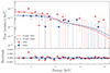 |
Fig. 2. X-ray XMM-Newton EPIC combined folded spectra of BB1 (filled red circles) and BB8 (filled blue squares) overplotted with their respective best-fit models (absorbed power-law) in dashed red for BB1 and dot-dashed blue for BB8. The residuals after the model subtraction are plotted in the bottom panel. The plotted data are binned to 20 counts per bin using the setplotrebin tool in XSPEC for plotting purposes only (the fitting was done with data only binned to have at least one count per bin). |
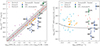 |
Fig. 3. X-ray luminosity as a function of SFR, metallicity, and sSFR for the BBs and comparison samples. Left: X-ray luminosity LX as a function of SFR and metallicity for the BBs (filled blue squares and down-arrows) studied by XMM-Newton. The empirical relation by Brorby et al. (2016) is shown as a red dot-dashed line and its 1σ deviation as a grey region. Right: Our BB sample in the diagram of the X-ray luminosity over the SFR as dependent on the sSFR. The solid horizontal line represents the Lehmer et al. (2010) relation. The GP sample by Svoboda et al. (2019) (filled green squares and down-arrows) is plotted in both diagrams for comparison, along with a few other samples of Mineo et al. (2012) (filled turquoise circles only in the right plot), Douna et al. (2015) (filled purple circles only in the left plot), Brorby et al. (2016) (filled pink circles), and Fornasini et al. (2020) (filled dark yellow circles). |
A possible source for the large scatter of our BB sample may be the stochastic sampling of individual XRBs associated with the galaxies. To investigate this assumption, we performed a simulation study following a similar approach as in Anastasopoulou et al. (2019), Kouroumpatzakis et al. (2021), and Kyritsis et al. (2024). In particular, by using the SFR and gas-phase metallicity of each galaxy (Table 1) and integrating their corresponding metallicity-dependent XLFs from Lehmer et al. (2021) (L21), we calculated the expected number of HMXBs for each galaxy as follows:
For the integration of the L21 XLF, we assumed their best-fit parameters (from their Table 2), and the integration limits spanned between the Lmin = 1036 erg s−1 and Lmax = 5 × 1041 erg s−1, representing the minimum and maximum luminosity, respectively. Subsequently, by sampling from a Poisson distribution with a mean equal to the number of expected HMXBs calculated above, we generated 20 000 draws of the expected number of HMXBs ( ). Then we sampled the HMXB XLF of each galaxy by drawing the corresponding X-ray luminosities of
  sources each time. The total X-ray luminosity for each of the 20 000 simulations was then computed by summing the luminosity of each source drawn from the XLF for each instance.
This analysis allowed us to simulate the X-ray emission of 20 000 galaxies, considering the typical properties (SFR and metallicity) of the galaxies in our sample. At the same time, we accounted for fluctuations in the number of sources within each galaxy and stochastic effects associated with the sampling of their XLF. For each of these distributions, we calculated the mode and the 90%, 99%, and 99.9% upper and lower confidence intervals (CIs). The probability of the X-ray luminosity of a given galaxy being greater or smaller than the observed value is given in Table B.1, and the probability distributions based on the stochastic sampling are plotted in Fig. B.1.
In Fig. 4, we present the 90%, 99%, and 99.9% CIs of the total expected X-ray luminosity per SFR distribution due to the stochastic sampling of the HMXB XLF from L21, as a function of the metallicity of each galaxy in our sample. We also show in blue the BB sample of this work and in green the GP sample from Svoboda et al. (2019). For comparison, we overplot the scaling relations from Brorby et al. (2016), Fornasini et al. (2020), and Lehmer et al. (2021). Only one of the BBs, BB8, is above the empirical relation by Lehmer et al. (2021). More specifically, the probability of its luminosity being an outcome of stochastic behaviour is less than 1.2%. On the contrary, the rest of the BBs are significantly below the relation. BB5’s upper limit is within the 90% CI from the expected value, but all the other upper limits are beyond it. The detected BB1 and the upper limits of BB2 and BB7 lie in the 99% CI region. Two sources, BB3 and BB4, have their upper limits even beyond the lower bound of 99.9% and thus cannot be attributed to stochasticity effects at all. The jump in the distribution between BB2 and BB4 is due to them having the same metallicity, but different SFRs. The two bright GPs both lie beyond the upper bounds of the stochasticity sampling. The upper limit of the weakest GP, on the other hand, seems to be consistent with the Lehmer et al. (2021) relation.
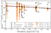 |
Fig. 4. Distribution of the total expected X-ray luminosity per SFR due to the stochastic sampling of the HMXB XLF from L21, as a function of the metallicity of each galaxy in our sample. Orange-, pink-, and goldenrod-shaded regions indicate the 90%, the 99%, and the 99.9% CI, respectively, of the expected LX/SFR distribution of each BB. Filled blue squares and down-arrows indicate the BB sample of this work. We also plot with filled green squares and down-arrows the GP sample from Svoboda et al. (2019). For comparison, we overplot with a red dot-dashed line the scaling relation from Brorby et al. (2016), with a grey dashed line the relation from Fornasini et al. (2020), and with a black dashed line the relation from Lehmer et al. (2021). |
4. Discussion
In this paper, we study the first X-ray observations of the extremely low-metallicity compact and highly star-forming young galaxies, the BBs. The X-ray data were obtained with the XMM-Newton satellite. The planned exposures were calculated to be sufficient for the detection of the expected X-ray flux based on empirical relations between X-ray flux, star formation, and metallicity. However, only two out of seven sources were detected (with one non-detection probably due to high background flare contamination). For the two detected sources, the X-ray flux and luminosity could be properly measured and the spectral fitting applied.
The luminosity of these two detected sources is about log LX ≈ 40.5 erg s−1, with one (BB1) being close to the expected luminosity estimated from empirical relations for star-forming galaxies, and the other (BB8) showing an X-ray excess five times the expected value. To explore the possibility of contamination from a background AGN or source confusion, we adopted a method similar to Svoboda et al. (2019). We estimated the number of background sources expected to have the same flux as the two BBs, which corresponds to the detection probability of such background AGNs. The BB fluxes in the 0.5−2 keV band are log FX ≈ −14.5 erg s−1 cm−2 for BB1 and log FX ≈ −14.6 erg s−1 cm−2 for BB8, which can then be compared to the values in Table 3 in Mateos et al. (2008). Given the higher probability of finding a fainter source, we used the values for a flux of log FX ≈ −14.7 erg s−1 cm−2. For an area of 1 deg2, the probability of finding a source with this flux is N(> S)≈474 (Mateos et al. 2008). For our source extraction regions of 30 arcsec (0.00022 deg2), this translates to N(> S)≈0.1. Therefore, the probability of finding a random background AGN in our source regions is quite low. The only nearby source is the star 13 arcsec south of BB1 (as classified by the SDSS DR16 SkyServer), but it is not expected to contribute to the X-ray flux at all.
Two sources, BB1 and BB2, were previously measured by a targeted Chandra observation (Wang et al. 2016). BB1 was detected with a measured flux by Wang et al. (2016), and its luminosity was constrained by Latimer et al. (2021) to be log LX ≈ 40.5 erg s−1 in the 0.5−2 keV band and log LX ≈ 40.8 erg s−1 in the 2−10 keV band. For the rest of the BBs, which were undetected by the standard methods, only the Bayesian-based upper limits on X-ray flux and luminosity were obtained. The upper limits of the luminosity of these sources are typically less than 1040 erg s−1.
The fact that our sample of BBs is mostly X-ray underluminous compared to the empirical relations using their SFR, stellar mass, and metallicity values is a somewhat surprising result. The relation by Brorby et al. (2016) was built for galaxies dominated by HMXBs– that is, the young star-forming galaxies. The sSFRs of BBs range from −7.9 to −7.5 (see Fig. 3), which is extremely high, signifying that the BBs are very young and star-forming galaxies and putting them far into the HMXB-dominated region (sSFRs > −10). Following the previous study of GPs (Svoboda et al. 2019), which found a significant X-ray excess in two out of three sources, an enhanced X-ray luminosity of BBs in more than one source could have been expected, especially since the BBs are more extreme than GPs. However, our results suggest the opposite: the BBs do not follow the empirical laws for local star-forming galaxies and could have lower X-ray luminosity on average. This result indicates that the higher emission of BB8 and the two GPs is likely not due to pure star formation activity.
For the two GPs, Svoboda et al. (2019) proposed that the enhanced X-ray luminosity can be attributed to a hidden AGN. The X-ray emission was too large to be produced by a standard XRB population. Both a larger population of X-ray binaries or ULXs were considered but concluded as unlikely since the GPs have an X-ray luminosity of the order of ∼1042 erg s−1 (Svoboda et al. 2019), which is too high even for ULXs with their typical X-ray luminosity of the order of ∼1039 erg s−1 (e.g. Kaaret et al. 2017). For BB8, the X-ray luminosity ∼1040 erg s−1 is not as high, and the enhanced luminosity could be due to an additional X-ray source (several ULXs, a bright ULX, or a larger population of HMXBs). However, we note that the stochasticity simulations do include contributions from ULXs, and therefore only the rare extreme ULXs would be a possibility for the high X-ray emission explanation.
We compared the measured luminosity and upper limits of observed BBs to different empirical relations by Lehmer et al. (2010, 2021), Brorby et al. (2016), and Fornasini et al. (2020), but with similar conclusions. Our BB8 shows enhanced X-ray luminosity with respect to all considered relations and is inconsistent at a confidence level of almost 99% with the expectations resulting from the stochastic sampling of the HMXB XLF. The X-ray luminosity of BB1 is either below or consistent with each relation, and the upper limits of the rest (BB2−BB7) are mostly below the empirical curves (see Figs. 3 and 4). The deviation is seemingly less pronounced for the relation by Lehmer et al. (2010), shown in the right panel of Fig. 3. However, this is likely just coincident, since the other samples are more appropriate for comparison with BBs that are largely in the HMXB-dominated regime (log(sSFR) > − 10). The relation by Lehmer et al. (2010) considered both LMXBs and HMXBs, while Brorby et al. (2016) and Lehmer et al. (2021) focused their sample only on the galaxies whose X-ray flux is dominated by HMXBs and also took into account the effects of metallicity (though in Lehmer et al. 2010, the stellar mass is taken into account and thus the metallicity is indirectly considered through the mass-metallicity relation by Tremonti et al. 2004). The lowest-metallicity source BB5 was too underexposed to have a robust detection due to high background flares. Nevertheless, this source is illustrative of how significant the metallicity effect is in the considered empirical relations. Compared to Lehmer et al. (2010), the upper limit is consistent with the expected X-ray luminosity. However, it is below the empirical relations that took the metallicity directly into account.
The extremely high sSFRs of BBs indicate that their dominating stellar population is very young, much younger than the star-forming galaxies used for the empirical relations. This leads to a hypothesis that our BBs may not be old enough to give rise to a significant population of X-ray binaries. This effect was studied by Shtykovskiy & Gilfanov (2007), Antoniou et al. (2010, 2019) for BeXRBs in the Magellanic Clouds. They showed that for a population of 10 Myr, there is an order of magnitude fewer HMXBs than in a population of 40 Myr. However, Fragos et al. (2013) showed that for XRB populations younger than 10 Myr, the X-ray luminosity seems to be higher, as the HMXBs tend to be more luminous. Therefore, our BBs would have to be even younger (probably less than 5 Myr) for this to have a significant effect. As Linden et al. (2010) showed, the characteristics and star formation history of young populations of bright HMXBs depend strongly on metallicity and formation channels. Thus, this could also be an effect in our galaxy sample, as our metallicities are rather low (log(O/H) + 12 < 8.1). Although we do not know the exact star formation history or stellar population ages of our studied sources, if the high sSFR of BBs indicates that their stellar populations are extremely young, this might be a reason for the deficit of the X-ray luminosity, especially for BB4, which is significantly below the empirical relations, even after taking the stochasticity into account (see Fig. 4). A detailed analysis of the optical spectra of these galaxies could provide insights into their star formation histories and help explain the observed low X-ray luminosities.
The obtained results might also be relevant for the high-redshift galaxies at the epoch of reionisation. The BBs, with their extreme sSFR due to high SFR and compactness, can be considered reminiscent of the first early-Universe galaxies, similarly to GPs, whose spectra are noticeably similar to the early high-redshift galaxies as recently observed by JWST (Schaerer et al. 2022; Rhoads et al. 2023). The higher X-ray flux of BB8, especially when compared to the other X-ray underluminous BBs, might suggest an alternative explanation: the elevated X-ray flux could be due to AGN activity, as was proposed for two GPs. But only for the GPs, the stochasticity effects cannot explain the elevation at more than a 99.9% confidence level (see Fig. 4), and the AGN scenario thus remains one of the most viable interpretations for these two GPs.
The presence of AGNs in dwarf galaxies has been revealed in several other sources (Greene & Ho 2004; Reines et al. 2013; Mezcua et al. 2018, 2023; Mezcua & Domínguez Sánchez 2020; Birchall et al. 2020; Reines 2022). Nonetheless, AGNs in dwarf galaxies are difficult to detect, as they are expected to be intrinsically low luminosity. Their X-ray luminosities are expected to be lower than ∼1040 or ∼1041 erg s−1, with a significant contribution from the thermal emission attributed to star formation that contaminates the signal at lower energies. Cases of AGNs in low-metallicity compact galaxies with extremely high sSFRs, such as GPs and BBs, are very rare and can improve our knowledge of the first galaxies in the Universe and their evolution and help us properly understand the crucial source of the ionising radiation during the cosmic reionisation. A more detailed investigation of potential AGN candidates among them, as well as a systematic analysis of a larger sample of these local analogues, is needed to shed light on the power of the galaxies in the early Universe. One such method might include the optical variability of these sources, as studied by Baldassare et al. (2018, 2020).
5. Conclusions
We studied seven BBs in X-rays using data from the XMM-Newton satellite. Only two sources were detected, and we were able to obtain their X-ray luminosity. The luminosity was constrained to be log LX = 40.5 ± 0.3 erg s−1 for BB1 and log LX = 40.4 ± 0.2 erg s−1 for BB8. For the remaining sources, only the Bayesian-based upper limits were measured. One source (BB3) has an X-ray luminosity upper limit of log LX < 40.2 erg s−1, while the rest are below log LX ∼ 39.9 erg s−1. Comparison with different empirical relations showed that, except for the brightest source (BB8), the X-ray luminosities of the BBs are below those predicted by empirical relations. By applying the stochasticity analysis, we show that the brightest source (BB8) is, at a 99% confidence level, inconsistent with the expectations, which could hint at the presence of an additional X-ray source, such as an AGN or an extreme ULX. On the contrary, the second detected source (BB1) is, at more than 99%, inconsistent with the lower bounds of the stochasticity sampling. Two sources (BB3 and BB4) are completely outside the lower bounds and therefore cannot be explained by the stochasticity with more than 99.9% probability. Therefore, our results indicate that the BBs have much larger scatter and/or are markedly X-ray underluminous. The insufficient X-ray luminosity might be due to the BBs not having had enough time to develop a significant XRB population. A larger sample of BBs, combined with their optical spectra and variability measurements, would enhance our understanding of these sources.
See the guide at: https://www.cosmos.esa.int/web/xmm-newton/sas-thread-images
See the XSPEC manual by Arnaud et al. (2022).
Acknowledgments
We sincerely thank the anonymous referee for their insightful comments, which have significantly improved the quality of the manuscript. This work was supported by the Czech Science Foundation project No. 22-22643S. MC and POP were partly supported by the High Energy National Programme (PNHE) of the French National Center of Scientific Research (CNRS) and the French Spatial Agency (CNES). Software used: Numpy (Harris et al. 2020), matplotlib (Hunter 2007), astropy (Astropy Collaboration 2013, 2018, 2022).
References
- Anastasopoulou, K., Zezas, A., Gkiokas, V., & Kovlakas, K. 2019, MNRAS, 483, 711 [NASA ADS] [CrossRef] [Google Scholar]
- Anders, E., & Grevesse, N. 1989, Geochim. Cosmochim. Acta, 53, 197 [Google Scholar]
- Antoniou, V., Zezas, A., Hatzidimitriou, D., & Kalogera, V. 2010, ApJ, 716, L140 [NASA ADS] [CrossRef] [Google Scholar]
- Antoniou, V., Zezas, A., Drake, J. J., et al. 2019, ApJ, 887, 20 [NASA ADS] [CrossRef] [Google Scholar]
- Arnaud, K. 1996, ASP Conf. Ser., 101, 17 [NASA ADS] [Google Scholar]
- Arnaud, K., Gordon, C., Dorman, B., & Rutkowski, K. 2022, XSPEC, An X-Ray Spectral Fitting Package, Users’ Guide for version 12.13, HEASARC [Google Scholar]
- Astropy Collaboration (Robitaille, T. P., et al.) 2013, A&A, 558, A33 [NASA ADS] [CrossRef] [EDP Sciences] [Google Scholar]
- Astropy Collaboration (Price-Whelan, A. M., et al.) 2018, AJ, 156, 123 [Google Scholar]
- Astropy Collaboration (Price-Whelan, A. M., et al.) 2022, ApJ, 935, 167 [NASA ADS] [CrossRef] [Google Scholar]
- Baldassare, V. F., Geha, M., & Greene, J. 2018, ApJ, 868, 152 [NASA ADS] [CrossRef] [Google Scholar]
- Baldassare, V. F., Dickey, C., Geha, M., & Reines, A. E. 2020, ApJ, 898, L3 [NASA ADS] [CrossRef] [Google Scholar]
- Basu-Zych, A. R., Lehmer, B. D., Hornschemeier, A. E., et al. 2013, ApJ, 762, 45 [NASA ADS] [CrossRef] [Google Scholar]
- Birchall, K. L., Watson, M. G., & Aird, J. 2020, MNRAS, 492, 2268 [NASA ADS] [CrossRef] [Google Scholar]
- Brorby, M., Kaaret, P., Prestwich, A., & Mirabel, I. F. 2016, MNRAS, 457, 4081 [NASA ADS] [CrossRef] [Google Scholar]
- Cardamone, C., Schawinski, K., Sarzi, M., et al. 2009, MNRAS, 399, 1191 [NASA ADS] [CrossRef] [Google Scholar]
- Douna, V. M., Pellizza, L. J., Mirabel, I. F., & Pedrosa, S. E. 2015, A&A, 579, A44 [NASA ADS] [CrossRef] [EDP Sciences] [Google Scholar]
- Finkelstein, S. L., Bagley, M. B., Ferguson, H. C., et al. 2023, ApJ, 946, L13 [NASA ADS] [CrossRef] [Google Scholar]
- Fornasini, F. M., Civano, F., & Suh, H. 2020, MNRAS, 495, 771 [NASA ADS] [CrossRef] [Google Scholar]
- Fragos, T., Lehmer, B., Tremmel, M., et al. 2013, ApJ, 764, 41 [NASA ADS] [CrossRef] [Google Scholar]
- Franeck, A., Wünsch, R., Martínez-González, S., et al. 2022, ApJ, 927, 212 [NASA ADS] [CrossRef] [Google Scholar]
- Gabriel, C., Denby, M., Fyfe, D., et al. 2004, ASP Conf. Ser., 314, 759 [NASA ADS] [Google Scholar]
- Greene, J. E., & Ho, L. C. 2004, ApJ, 610, 722 [NASA ADS] [CrossRef] [Google Scholar]
- Grimm, H.-J., Gilfanov, M., & Sunyaev, R. 2003, MNRAS, 339, 793 [NASA ADS] [CrossRef] [Google Scholar]
- Harikane, Y., Ouchi, M., Oguri, M., et al. 2023, ApJS, 265, 5 [NASA ADS] [CrossRef] [Google Scholar]
- Harris, C. R., Millman, K. J., van der Walt, S. J., et al. 2020, Nature, 585, 357 [NASA ADS] [CrossRef] [Google Scholar]
- Henry, A., Scarlata, C., Martin, C., & Erb, D. 2015, ApJ, 809, 19 [NASA ADS] [CrossRef] [Google Scholar]
- Hunter, J. D. 2007, Comput. Sci. Eng., 9, 90 [NASA ADS] [CrossRef] [Google Scholar]
- Izotov, Y., Schaerer, D., Thuan, T. X., et al. 2016, MNRAS, 461, 3683 [CrossRef] [Google Scholar]
- Izotov, Y., Schaerer, D., Worseck, G., et al. 2018a, MNRAS, 474, 4514 [NASA ADS] [CrossRef] [Google Scholar]
- Izotov, Y., Worseck, G., Schaerer, D., et al. 2018b, MNRAS, 478, 4851 [CrossRef] [Google Scholar]
- Jaskot, A., Dowd, T., Oey, M. S., Scarlata, C., & McKinney, J. 2019, ApJ, 885, 96 [NASA ADS] [CrossRef] [Google Scholar]
- Joye, W. A., & Mandel, E. 2003, ASP Conf. Ser., 295, 489 [Google Scholar]
- Kaaret, P., Brorby, M., Casella, L., & Prestwich, A. H. 2017, MNRAS, 471, 4234 [CrossRef] [Google Scholar]
- Kouroumpatzakis, K., Zezas, A., Wolter, A., et al. 2021, MNRAS, 500, 962 [Google Scholar]
- Kroupa, P. 2001, MNRAS, 322, 231 [NASA ADS] [CrossRef] [Google Scholar]
- Kyritsis, E., Zezas, A., Haberl, F., et al. 2024, A&A, submitted [arXiv:2402.12367] [Google Scholar]
- Latimer, L. J., Reines, A. E., Hainline, K. N., Greene, J. E., & Stern, D. 2021, ApJ, 914, 133 [NASA ADS] [CrossRef] [Google Scholar]
- Lehmer, B. D., Alexander, D. M., Bauer, F., et al. 2010, ApJ, 724, 559 [NASA ADS] [CrossRef] [Google Scholar]
- Lehmer, B. D., Eufrasio, R. T., Basu-Zych, A., et al. 2021, ApJ, 907, 17 [NASA ADS] [CrossRef] [Google Scholar]
- Linden, T., Kalogera, V., Sepinsky, J. F., et al. 2010, ApJ, 725, 1984 [Google Scholar]
- Madau, P., & Dickinson, M. 2014, ARA&A, 52, 415 [Google Scholar]
- Mateos, S., Warwick, R. S., Carrera, F. J., et al. 2008, A&A, 492, 51 [NASA ADS] [CrossRef] [EDP Sciences] [Google Scholar]
- McKinney, J. H., Jaskot, A., Oey, M. S., et al. 2019, ApJ, 874, 52 [NASA ADS] [CrossRef] [Google Scholar]
- Mezcua, M., Civano, F., Fabbiano, G., Miyaji, T., & Marchesi, S. 2016, ApJ, 817, 20 [Google Scholar]
- Mezcua, M., Civano, F., Marchesi, S., et al. 2018, MNRAS, 478, 2576 [NASA ADS] [CrossRef] [Google Scholar]
- Mezcua, M., & Domínguez Sánchez, H. 2020, ApJ, 898, L30 [Google Scholar]
- Mezcua, M., Siudek, M., Suh, H., et al. 2023, ApJ, 943, L5 [NASA ADS] [CrossRef] [Google Scholar]
- Mineo, S., Gilfanov, M., & Sunyaev, R. 2012, MNRAS, 419, 2095 [Google Scholar]
- Orlitová, I., Verhamme, A., Henry, A., et al. 2018, A&A, 616, A60 [Google Scholar]
- Park, T., Kashyap, V. L., Siemiginowska, A., et al. 2006, ApJ, 652, 610 [Google Scholar]
- Pettini, M., & Pagel, B. E. J. 2004, MNRAS, 348, L59 [NASA ADS] [CrossRef] [Google Scholar]
- Planck Collaboration VI. 2020, A&A, 641, A6 [NASA ADS] [CrossRef] [EDP Sciences] [Google Scholar]
- Ranalli, P., Comastri, A., & Setti, G. 2003, A&A, 399, 39 [NASA ADS] [CrossRef] [EDP Sciences] [Google Scholar]
- Reines, A. E. 2022, Nat. Astron., 6, 26 [NASA ADS] [CrossRef] [Google Scholar]
- Reines, A. E., Greene, J. E., & Geha, M. 2013, ApJ, 775, 116 [Google Scholar]
- Rhoads, J. E., Wold, I. G. B., Harish, S., et al. 2023, ApJ, 942, L14 [NASA ADS] [CrossRef] [Google Scholar]
- Robertson, B. E., Ellis, R. S., Dunlop, J. S., McLure, R. J., & Stark, D. P. 2010, Nature, 468, 49 [Google Scholar]
- Salpeter, E. E. 1955, ApJ, 121, 161 [Google Scholar]
- Schaerer, D., Marques-Chaves, R., Barrufet, L., et al. 2022, A&A, 665, L4 [NASA ADS] [CrossRef] [EDP Sciences] [Google Scholar]
- Shtykovskiy, P. E., & Gilfanov, M. R. 2007, Astron. Lett., 33, 437 [NASA ADS] [CrossRef] [Google Scholar]
- Smith, M., & Guainazzi, M. 2022, XMM-Newton Calibration Technical Note, EPIC Status of Calibration and Data Analysis, XMM-SOC-CAL-TN-0018 [Google Scholar]
- Svoboda, J., Douna, V., Orlitová, I., & Ehle, M. 2019, ApJ, 880, 144 [NASA ADS] [CrossRef] [Google Scholar]
- Tremonti, C. A., Heckman, T., Kauffmann, G., et al. 2004, ApJ, 613, 898 [CrossRef] [Google Scholar]
- Verhamme, A., Orlitová, I., Schaerer, D., et al. 2017, A&A, 597, A13 [NASA ADS] [CrossRef] [EDP Sciences] [Google Scholar]
- Verner, D. A., Ferland, G. J., Korista, K. T., & Yakovlev, D. G. 1996, ApJ, 465, 487 [Google Scholar]
- Wachter, K., Leach, R., & Kellogg, E. 1979, ApJ, 230, 274 [NASA ADS] [CrossRef] [Google Scholar]
- Wang, S., Liu, J., Qiu, Y., et al. 2016, ApJS, 224, 40 [Google Scholar]
- Yang, H., Malhotra, S., Rhoads, J. E., & Wang, J. 2017, ApJ, 847, 38 [NASA ADS] [CrossRef] [Google Scholar]
Appendix A: Details of source and background regions
The details of the source and different background extraction regions for all seven BBs are summarised in Table A.1.
Details of the source and background extraction regions
Appendix B: Stochasticity probabilities and X-ray luminosity distributions
The results of the probability analysis of the stochasticity sampling are summarised in Table B.1, where the probability of stochastically observing a galaxy having the same properties as the observed one, with X-ray luminosity greater or smaller than the observed value, is given. In addition, in Fig. B.1, we plot the histograms of the X-ray luminosity distribution over SFR based on the stochasticity simulations.
Probability for a galaxy, with the same physical properties as the observed one, having X-ray luminosity greater or less than the observed value (i.e. Lx> Lobs or Lx< Lobs) due to stochastic sampling
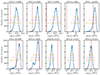 |
Fig. B.1. Histograms of the X-ray luminosity distribution over SFR based on the stochasticity simulations for seven BBs and three GPs. The red dashed line indicates the observed X-ray luminosity. The orange, pink and goldenrod bars indicate the lower and upper bounds of the CI 90%, 99%, and 99.9%. |
All Tables
Probability for a galaxy, with the same physical properties as the observed one, having X-ray luminosity greater or less than the observed value (i.e. Lx> Lobs or Lx< Lobs) due to stochastic sampling
All Figures
|
Fig. 1. X-ray vignetting-corrected background-subtracted images for BB1 (left) and BB8 (right) in the three used energy bands, 0.5–1 keV, 1–2 keV, and 2–10 keV (from top left to bottom left), and the SDSS optical images (bottom right). The source extraction regions (solid white open circles) and background regions (dot-dashed white open circles) are denoted in the figures (see the appendix for details of the extraction regions). The dashed green open rectangles, present in each X-ray image, indicate the regions corresponding to the SDSS images. The X-ray images are given in linear scale using the minima and maxima of the image cutouts. The colour scale denotes the pixel intensity, i.e. the scaled and weighted count rate per pixel. The SDSS images are shown at a different size scale than the X-ray images since a larger field of view would not provide adequate detail of the galaxies. |
| In the text | |
|
Fig. 2. X-ray XMM-Newton EPIC combined folded spectra of BB1 (filled red circles) and BB8 (filled blue squares) overplotted with their respective best-fit models (absorbed power-law) in dashed red for BB1 and dot-dashed blue for BB8. The residuals after the model subtraction are plotted in the bottom panel. The plotted data are binned to 20 counts per bin using the setplotrebin tool in XSPEC for plotting purposes only (the fitting was done with data only binned to have at least one count per bin). |
| In the text | |
|
Fig. 3. X-ray luminosity as a function of SFR, metallicity, and sSFR for the BBs and comparison samples. Left: X-ray luminosity LX as a function of SFR and metallicity for the BBs (filled blue squares and down-arrows) studied by XMM-Newton. The empirical relation by Brorby et al. (2016) is shown as a red dot-dashed line and its 1σ deviation as a grey region. Right: Our BB sample in the diagram of the X-ray luminosity over the SFR as dependent on the sSFR. The solid horizontal line represents the Lehmer et al. (2010) relation. The GP sample by Svoboda et al. (2019) (filled green squares and down-arrows) is plotted in both diagrams for comparison, along with a few other samples of Mineo et al. (2012) (filled turquoise circles only in the right plot), Douna et al. (2015) (filled purple circles only in the left plot), Brorby et al. (2016) (filled pink circles), and Fornasini et al. (2020) (filled dark yellow circles). |
| In the text | |
|
Fig. 4. Distribution of the total expected X-ray luminosity per SFR due to the stochastic sampling of the HMXB XLF from L21, as a function of the metallicity of each galaxy in our sample. Orange-, pink-, and goldenrod-shaded regions indicate the 90%, the 99%, and the 99.9% CI, respectively, of the expected LX/SFR distribution of each BB. Filled blue squares and down-arrows indicate the BB sample of this work. We also plot with filled green squares and down-arrows the GP sample from Svoboda et al. (2019). For comparison, we overplot with a red dot-dashed line the scaling relation from Brorby et al. (2016), with a grey dashed line the relation from Fornasini et al. (2020), and with a black dashed line the relation from Lehmer et al. (2021). |
| In the text | |
|
Fig. B.1. Histograms of the X-ray luminosity distribution over SFR based on the stochasticity simulations for seven BBs and three GPs. The red dashed line indicates the observed X-ray luminosity. The orange, pink and goldenrod bars indicate the lower and upper bounds of the CI 90%, 99%, and 99.9%. |
| In the text | |
Current usage metrics show cumulative count of Article Views (full-text article views including HTML views, PDF and ePub downloads, according to the available data) and Abstracts Views on Vision4Press platform.
Data correspond to usage on the plateform after 2015. The current usage metrics is available 48-96 hours after online publication and is updated daily on week days.
Initial download of the metrics may take a while.