| Issue |
A&A
Volume 689, September 2024
|
|
|---|---|---|
| Article Number | A170 | |
| Number of page(s) | 13 | |
| Section | Extragalactic astronomy | |
| DOI | https://doi.org/10.1051/0004-6361/202449406 | |
| Published online | 12 September 2024 | |
The origin of the X-ray luminosity of the green pea galaxies: X-ray binaries or active galactic nuclei?
1
Kavli Institute for Astronomy and Astrophysics, Peking University, Beijing 100871, People’s Republic of China
2
CAS Key Laboratory of Optical Astronomy, National Astronomical Observatories, Beijing 100101, China
3
School of Astronomy and Space Science, University of Chinese Academy of Sciences, Beijing 101408, China
4
University of Chinese Academy of Sciences, Nanjing, Jiangsu 211135, China
5
Key Laboratory for Research in Galaxies and Cosmology, Shanghai Astronomical Observatory, Chinese Academy of Sciences, 80 Nandan Road, Shanghai 200030, China
6
School of Astronomy and Space Sciences, University of Chinese Academy of Sciences, Beijing 100049, China
7
Leiden Observatory, Leiden University, PO Box 9513, 2300 RA Leiden, The Netherlands
8
Kapteyn Astronomical Institute, University of Groningen, PO Box 800, 9700 AV Groningen, The Netherlands
Received:
30
January
2024
Accepted:
10
June
2024
Context. Green pea galaxies (GPs) are renowned for their compact sizes, low masses, strong emission lines, high star formation rates (SFRs), and being analogs to high-z Lyα-emitting galaxies.
Aims. This investigation focuses on a curated sample of six GPs with X-ray detections, sourced from XMM-Newton, Swift, Chandra and eROSITA, with the aim to elucidate the origin of their X-ray luminosity.
Methods. We determined the GPs’ physical properties, including the SFRs, stellar masses, and metallicities, based on multiwavelength photometry and LAMOST spectra analysis.
Results. Within the LX–SFR relation, GPs predominantly occupy the high specific SFR domain, where high-mass X-ray binaries (HMXBs) dominate, leading to an excess in X-ray luminosity compared to the sole contributions from HMXBs (LXHMXB). Moreover, GPs exhibit a noticeable excess in X-ray luminosity within the LX–SFR–metallicity relationship. The cumulative input from X-ray binaries, hot gas, hot interstellar medium, and young stellar objects falls short in accounting for the X-ray luminosity observed in GPs. The presence of active galactic nucleus (AGNs) surfaces is suggested based on mid-infrared color–color criteria. Furthermore, based on the MBH derived from LAMOST optical spectra, GPs conform to the MBH–M⋆ scaling relation.
Conclusions. The origin of the X-ray excess likely stems from the combined contributions of HMXBs and AGNs, although further scrutiny via X-ray spectra and spatially resolved imaging using forthcoming facilities is needed to confirm this.
Key words: galaxies: peculiar / galaxies: starburst
© The Authors 2024
 Open Access article, published by EDP Sciences, under the terms of the Creative Commons Attribution License (https://creativecommons.org/licenses/by/4.0), which permits unrestricted use, distribution, and reproduction in any medium, provided the original work is properly cited.
This article is published in open access under the Subscribe to Open model. Subscribe to A&A to support open access publication.
1. Introduction
Galaxy-wide X-ray emissions come from a variety of sources: X-ray binaries (XRBs), supernovae, supernova remnants, hot interstellar gas (≈0.2 − 1 keV), massive stars, and active galactic nuclei (AGNs). Extensive studies have revealed a robust correlation between galaxy-wide X-ray emissions and the total star formation rate (SFR), as described by the LX–SFR relation (Grimm et al. 2003; Ranalli et al. 2003; Gilfanov et al. 2004a,b; Persic et al. 2004; Persic & Rephaeli 2007). The prevailing factor driving the LX–SFR relationship appears to be emissions primarily stemming from XRBs, particularly within the 2–10 keV energy range, where contributions from hot interstellar gas and young stars are negligible. Colbert et al. (2004) analyzed point-source populations in 32 nearby spiral and elliptical galaxies using Chandra, demonstrating a linear correlation between the galaxy-wide X-ray luminosity from these sources, and both the SFR and stellar mass (M⋆). The relative contribution from high-mass X-ray binaries (HMXBs) and low-mass X-ray binaries (LMXBs) varies with specific SFRs (sSFRs). HMXBs are relatively short-lived, with lifetimes of 106 − 7 yr, and trace recent star formation, while the LMXBs trace older star formation on timescales of over 108 − 9 yr. The relative contribution of HMXBs and LMXBs to the galaxy-wide LX is determined by the specific star formation rate (sSFR). Lehmer et al. (2010) show that LX/SFR values in terms of sSFR are separated into two regimes: at low sSFRs (≤ 10−10 yr−1) both LMXBs and HMXBs contribute to the total LX, and at high sSFRs (> 10−10 yr−1) the LX is dominated by the contributions from HMXBs. As shown by Persic & Rephaeli (2007), Iwasawa et al. (2009), ultraluminous infrared galaxies (ULIRGs) with SFR > 100 M⊙ yr−1, exhibit a higher LX(2–10 keV)/SFR ratio compared to galaxies with considerably lower SFRs, indicating the dominance of HMXBs in the LX(2–10 keV) at high sSFR regime. Assuming that the galaxy-wide X-ray luminosity ( ) reflects emissions from both HMXBs and LMXBs and correlates linearly with the stellar mass and SFR, Lehmer et al. (2010) derived a relation in the form of
  , based on Chandra observations of 17 luminous infrared galaxies, where α = (9.05 ± 0.37) × 1028 erg s−1 M⊙ yr−1 and β = (1.62 ± 0.22) × 1039 erg s−1 (M⊙ yr−1) (also referenced in Colbert et al. 2004).
Subsequent studies (Basu-Zych et al. 2013a; Lehmer et al. 2016; Aird et al. 2016) demonstrate the evolving nature of the LX–SFR relation with redshift, a phenomenon corroborated by population synthesis predictions (Linden et al. 2010). Recent investigations (Brorby et al. 2014; Douna et al. 2015; Brorby et al. 2016; Lehmer et al. 2022) reveal that a reduced metallicity amplifies the LX/SFR ratio in HMXBs. Fornasini et al. (2019) conducted an analysis involving the stacking of X-ray data from galaxies at z ∼ 2, stratifying them based on varying metallicity levels, and uncovered an anticorrelation between LX/SFR and metallicity at this redshift, direct evidence of metallicity’s role in the redshift evolution of the  /SFR ratio and Fornasini et al. (2020), Lehmer et al. (2021) derived calibrated forms of
  –SFR versus metallicity (12+log(O/H)). The LX–SFR–metallicity relation (Fragos et al. 2013b; Brorby et al. 2016; Madau & Fragos 2017; Fornasini et al. 2020) holds significant implications for nebular ionization and the heating of the intergalactic medium in the early Universe. Population synthesis models of XRBs explicate the link between metallicity and
  /SFR in two main ways (Dray et al. 2006; Linden et al. 2010; Fragos et al. 2013a,b; Basu-Zych et al. 2013b): (1) diminished stellar winds in massive stars result in a higher retention of mass that evolves into black holes (BHs), thereby rendering a higher LX(BH-HMXB)/SFR compared to neutron star-HMXBs (Mapelli et al. 2009; Zampieri & Roberts 2009), and (2) reduced stellar winds lead to less angular momentum loss within binary systems, limiting orbital expansion. Consequently, these systems encounter Roche-lobe overflow with elevated accretion rates, and as such this mechanism is favored over Bondi-Hoyle wind accretion.
Green pea galaxies (GPs; Cardamone et al. 2009) are compact, isolated galaxies with high SFRs. Due to the limited number of spectroscopically confirmed GPs, there is a limited number of X-ray detections. Svoboda et al. (2019) analyzed the X-ray properties of three GPs (including two detected by XMM-Newton) and determined an upper limit for the X-ray luminosity. They deliberated on the excessive X-ray luminosity in GPs, which surpasses predicted values derived from the LX–SFR–metallicity relation. Based on the two GPs with X-ray detections, Kawamuro et al. (2019) documented X-ray observations of these two sources using NuSTAR in the hard X-ray range (> 10 keV) and XMM-Newton in the soft X-ray range (< 10 keV). They find no significant detection in the hard X-ray domain but robust emissions in the soft X-ray range. Svoboda et al. (2019) argue that even when accounting for contributions solely from star formation, a standard XRB population, and hot gas, the overall X-ray luminosity of GPs cannot be explained. Potential explanations for the observed X-ray excess include the presence of a concealed AGN, an expanded population of X-ray binaries, or ultraluminous X-ray sources. Kawamuro et al. (2019) propose that the excess X-ray emission might arise from pure star formation or a hypothetical AGN torus absorbing a significant portion of the X-ray emission.
The majority of massive galaxies harbor supermassive BHs within their central regions (Kormendy & Richstone 1995; Kormendy & Ho 2013). Harish et al. (2023) confirmed the presence of BHs in GPs using mid-infrared (MIR) variability. Furthermore, the X-ray excess observed in GPs might be accounted for by AGNs (Svoboda et al. 2019; Kawamuro et al. 2019).
We have compiled a sample of six GPs with identified X-ray detections to validate the observed X-ray excess and propose plausible explanations. In Sect. 2 we introduce the dataset and the specific samples utilized in this study, detailing the measured physical properties. In Sect. 3 we discuss the contributions originating from XRBs, BHs, hot gas, hot interstellar medium (ISM), and young stellar objects (YSOs). In Sect. 4 we explore the elevated  values observed at lower metallicities, and explain that one source with strong emission lines might be a starburst galaxy hosting a dust-obscured AGN. In Sect. 5 we summarize our work.
2. Data and sample
In this section we outline the procedures for sample selection, detail the methodology used to measure physical properties such as SFRs, metallicities, and stellar mass, and conduct a comprehensive analysis of a single source using X-ray spectra obtained from XMM-Newton.
2.1. Sample selection
Green pea galaxies are renowned for strong [O III]λ5007 emission lines in the r band. To select GPs with X-ray detections, we focused on compact galaxies with strong [O III]λ5007 emission lines reported in the LAMOST survey (Liu et al. 2022, 2023)1. Specifically, we limited our selection to sources with an equivalent width (EW) exceeding the lower threshold established by spectroscopically confirmed GPs in Cardamone et al. (2009), namely EW([O III]λ5007) > 12.6 Å. By cross-matching the LAMOST GPs with different X-ray surveys with a radius of 3 arcseconds, we obtained six sources with X-ray detections. Their properties are listed in Table 1.
Basic information about the GPs with X-ray detections.
Green pea galaxies with X-ray detections are identified in different X-ray surveys: 4XMM-Newton DR13 (Traulsen et al. 2020; Webb et al. 2020), Swift’s X-Ray Telescope (XRT) data (Burrows et al. 2005), Chandra Source Catalog (CSC) 2.0 (Evans et al. 2010), and the extended ROentgen Survey with an Imaging Telescope Array (eROSITA) Final Equatorial Depth Survey (eFEDS) X-ray catalog (Brunner et al. 2022). In this study we utilized measured fluxes within the observed frame’s energy bands: 0.2–12 keV for XMM-Newton, 0.3–10 keV for Swift, 0.5–7 keV for CSC 2.0, and 0.2–2.3 keV for eFEDS. Five sources with X-ray images, in conjunction with Sloan Digital Sky Survey (SDSS) images and LAMOST spectra, are presented in Fig. 1, and the source detected with eFEDS is presented in Fig. 2. Sect. 4.1 discusses the bias in this selection method.
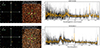 |
Fig. 1. Two GPs with X-ray detections from XMM-Newton (J1330-0043 and J0035+0431). Left panels: SDSS and XMM-Newton image cutouts. Right panels: LAMOST spectra. The black lines mark flux-calibrated spectra, the orange curves the spectra smoothed with a Gaussian kernel standard deviation of 3 pixels, and the gray-shaded regions the flux error. |
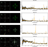 |
Fig. 2. GPs with X-ray detection from Swift (J0205+1504 and J0227+2355; top two rows), the GP with X-ray detection from Chandra (J1605+4405; third row), and the GP with X-ray detection from eROSITA (J0906+0242; bottom row). Left panels: SDSS, Swift, and Chandra image cutouts. Right panels: LAMOST spectra. The black lines mark the flux-calibrated spectrum, the orange curves the spectrum smoothed with a kernel of 3, and the gray-shaded regions the flux error. |
Furthermore, the k correction was applied with kcorr = (1 + z)Γ − 2. For the X-ray luminosity in the 0.5 − 8 keV range in the rest frame, we converted the observed values with the method based on the rest-frame energy limits using the following equation:
For the LX(0.5 − 8 keV) in the rest frame, we adopted the Γ = 2.02 in a single-power-law form, where different photon indices will not have a significant impact on the derived luminosity.
We used three additional GP samples from two previous studies (Svoboda et al. 2019; Kawamuro et al. 2019) for a comparative analysis of the origin of the X-ray luminosity. The fundamental details of these samples are summarized in Table 1.
2.2. Physical properties: SFR, metallicity, and stellar mass measurements
The spectral data obtained from LAMOST for all six GPs were deconstructed to determine the contribution from the BHs using the methodology outlined in QSOFITMORE (Fu 2021). The fitting results are presented in Fig. B.1.
To determine the stellar mass, age, and SFR, we performed fittings using CIGALE (Burgarella et al. 2005; Boquien et al. 2019; Yang et al. 2020, 2022) and multiwavelength photometry data. These data encompass inputs from various sources, such as X-ray surveys, Galaxy Evolution Explorer (GALEX) (Bianchi et al. 2017) far- and near-UV, SDSS ugriz bands, and All WISE Source Catalog (AllWISE) W1 to W4 (Wright et al. 2010, 2019). The fitting configuration involves several modules and models within CIGALE. These include the delayed-τ star formation history, BC03 stellar population models (Bruzual & Charlot 2003), the Chabrier initial mass function (Chabrier 2003), nebular emission lines, a modified starburst model accounting for dust attenuation, the dust emission model from Casey (2012), the SKIRTOR 2016 AGN model (Stalevski et al. 2012, 2016), and the xray module, which we used to take X-ray emissions into account. An example of the fitting result of the spectral energy distribution (SED) is shown in Fig. 3, and the remaining fitting results are shown in Fig. A.1. These figures showcase the output derived from the SED fitting process. The advantage of using the SFR determined from SED fitting results instead of the method used in Svoboda et al. (2019), the later of which combines IR and UV photometry based on the scaling relations from Hao et al. (2011), Kennicutt & Evans (2012), Durbala et al. (2020), is to calculate the SFR of the galaxy apart from the contributions from AGNs. For example, from the SED fitting result displayed in the Fig. 3, the stellar emission at 22 μm in Wide-field Infrared Survey Explorer (WISE) would be mainly emitted by the AGNs (by ∼2 orders of magnitude), which would dramatically overpredict the SFRs of the galaxies.
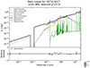 |
Fig. 3. CIGALE SED fitting result for source J0035+0431. |
Figure 4 presents the sources with corresponding emission line spectral coverage3 in the Baldwin, Philips, and Terlevich (BPT) diagram (Baldwin et al. 1981; Veilleux & Osterbrock 1987), according to the definitions in Kewley et al. (2001), Kauffmann et al. (2003), and Kewley et al. (2006). As discussed in Sect. 3.2.2, we used the flux ratios of the narrow emission lines.
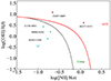 |
Fig. 4. BPT diagram of the GPs with spectral coverage. The plotting routine is based on that from Cherinka et al. (2019). |
In determining the metallicity, we treated the sources that are classified as star-forming and AGNs separately according to the BPT classification. For the star-forming sources, we used one of two methods – the O3N2 technique from Pettini & Pagel (2004), and the newly calibrated R23 method outlined in Jiang et al. (2019) – depending on if Hα and [N II]λ6584 emission lines are present within the LAMOST spectra. If these lines are detected, we employed the Pettini & Pagel (2004) O3N2 method, and if not the R23 method. It should be noted that our metallicity calculations are based on measurements obtained solely from the narrow-line components. For AGNs, we used the method from Schlegel et al. (1998), which works well for narrow-line regions of AGNs.
The physical properties of the GPs studied in this work are outlined in Table 2. The GPs studied in Kawamuro et al. (2019) are also included in Table 2 for comparison. In the following discussions, we employ the stellar mass, metallicity, SFR4, and X-ray luminosity measurements5 from Svoboda et al. (2019); we refer to the two GPs with X-ray detections from XMM-Newton as GP1 and GP2, and the one without X-ray detection as GP3.
Measured physical properties of GPs with X-ray detections.
We calculated the SFR ratios of log SFRNUV+IR/log SFRSED to lie in the range 0.34–1.38. The discrepancies mainly come from the contributions from the AGNs. Section 4.1 of Svoboda et al. (2019) discusses the impact of different data analysis methods, and the authors conclude that the X-ray excess is prominent in their GPs regardless of the SFR and metallicity estimators. Specifically for the SFR estimation, the SFRFUV/SFRHα ratios vary from 0.68 to 0.93 for GP1 and GP2 (Svoboda et al. 2019). Hunter et al. (2010) derive log SFRFUV/log SFRHα = 0.99, where the two SFR measurements provide comparable results. Brorby et al. (2014) obtain SFRNUV+IR/SFRFUV = 1.23. The X-ray excess is present in GP1 and GP2 for all of the conversions.
2.3. X-ray spectral analysis
Out of the four sources detected in 4XMM-Newton DR13, only one source has available X-ray spectra obtained from the pn-CCD camera (PN) detector within the European Photon Imaging Camera (EPIC) instrument. Employing a fitting engine, which functions as a wrapper over Sherpa modeling (Freeman et al. 2001), we conducted fits on this source using a single-power-law model. We used the Levenberg-Marquardt method for the fitting, employing the χ2 statistic along with variance computed from data amplitudes. The fitted spectra are displayed in Fig. 5, and the fitting results are listed in Table 3. For the other sources, there are too few X-ray photons detected to generate an X-ray spectrum.
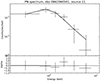 |
Fig. 5. X-ray flux from different energy bands for source J0035+0431, and the fitted spectra from XMM-Newton. |
Fitting result for the source with X-ray spectra.
3. Results
In this section we discuss the potential contributions from XRBs, AGNs, hot gas, hot ISM, and YSOs to the X-ray luminosity of the GPs.
3.1. Contributions from XRBs
The results in this subsection are provided in two parts: the traditionally investigated LX–SFR relation, and the LX–SFR–metallicity relation.
3.1.1. LX–SFR relation
In Fig. 6 we show LX measured in both the 0.5–8 keV and 2–10 keV (rest frame) energy bands to compare them with different scaling relations in the form of (Lehmer et al. 2010; Mineo et al. 2012b; Lehmer et al. 2019, 2022).
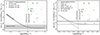 |
Fig. 6. Relations of the rest-frame X-ray luminosity in the 2–10 keV (left panel) and 0.5–8 keV energy bands (right panel) per SFR vs. sSFR. The green circles mark the GP measurements. Different LX–SFR relations in the form of Eq. (2) are marked in the left panel (Lehmer et al. 2010; Mineo et al. 2012b) and the right panel (Lehmer et al. 2019, 2022); the shaded regions mark the 1σ scatter. The gray downward pointing arrows indicate the upper limits of GPs with only limiting sensitivities from Chandra (see Sect. 4.1 for a discussion). The arrow size corresponds to the exposure time, with larger arrows indicating longer exposure times. The grayscale represents the source’s off-axis angle from the image center, with lighter shades indicating larger off-axis angles. |
Specifically, based on sub-galactic observations in bins of sSFR, Lehmer et al. (2019) fit X-ray luminosity functions, with the best-fitting result based on the clean samples as  and
and  . Unlike Lehmer et al. (2019), Lehmer et al. (2022) obtain the LX/SFR specifically for a sample of metal-poor galaxies (Z ≈ 0.3 Z⊙), obtaining a higher value. In both panels of Fig. 6, the GPs are located within the regime where HMXBs dominate (sSFRs > 10−10 yr−1) and LX/SFR excess is pronounced.
3.1.2. LX–SFR–metallicity relation
There are currently different LX–SFR–metallicity relations based on LX in different energy bands (Fragos et al. 2013b; Brorby et al. 2016; Fornasini et al. 2020; Lehmer et al. 2021). To avoid the impact of the conversion factor under different spectral shape assumptions, we compare the GPs separately in the following.
LX(0.5–8 keV)–SFR–metallicity relation. Brorby et al. (2016) fit the LX(0.5 − 8 keV)–SFR–metallicity relation to resolve the exceedingly high LX/SFR for Lyman break analog (LBA) galaxies. In this work, we also checked whether the GPs conform to the LX–SFR metallicity relation (see Fig. 7, where the green open circles lie above the predicted values in the LX–SFR–metallicity relation, with 1–2 dex offsets). The X-ray excess is also demonstrated in Svoboda et al. (2019), where the X-ray luminosity of the GPs is higher than the predicted values, with an excess of 1042 erg s−1.
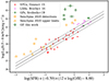 |
Fig. 7. LX–SFR–metallicity relation of the GPs. Green open circles with error bars represent the GPs in this study. The solid line denotes the best-fit LX–SFR–metallicity relation from Brorby et al. (2016), with dashed lines indicating a dispersion of σ = 0.34 dex. Red circles represent SFGs from Douna et al. (2015), and magenta squares represent LBAs from Brorby et al. (2016). Orange open circles indicate seven detections from Chandra observations, while orange triangles denote the four upper limits for low-redshift SFGs (Senchyna et al. 2020). |
We also compared samples from other studies with the GPs in this work. Douna et al. (2015) compiled a sample of 49 galaxies with measured SFRs, metallicities, and HMXB properties (observed number of sources and luminosities above some luminosity threshold) from the literature, building on previous samples from Mineo et al. (2012a) and Brorby et al. (2014). The selection criteria in Douna et al. (2015) are a high sSFR (> 10−10 yr−1) and a small distance (D < 65 Mpc). Brorby et al. (2016) used a sample of ten LBAs with metallicities in the range 12 + log(O/H) = 8.15 − 8.80 based on archival Chandra observations (Grimes et al. 2007; Basu-Zych et al. 2013b) and new observations. To ensure the exclusion of AGN contaminants within this sample, they conducted optical diagnostics (using a BPT diagram; Baldwin et al. 1981; Veilleux & Osterbrock 1987) and applied a 1.4 GHz spectral luminosity threshold.
LX(2–10 keV)–SFR–metallicity relation. Fornasini et al. (2020) derived a synthesized LX(2 − 10 keV)–SFR–metallicity relation based on star-forming galaxies (SFGs) at z = 0.1 − 0.9. Their analysis utilized stacked Chandra data from the Cosmic Evolution Survey (COSMOS) Legacy survey across three redshift bins. Along with the previously derived relations from Fragos et al. (2013b) and Madau & Fragos (2017), we compared the LX/SFR relation of the GPs with these scaling relations (see Fig. 8). Lyman-break galaxies (LBGs) from Basu-Zych et al. (2013b) are also included to demonstrate the relation.
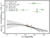 |
Fig. 8. LX/SFR–metallicity relation of the GPs. The green open circles with error bars mark the GPs in this work. Scaling relations from Fragos et al. (2013b), Madau & Fragos (2017), and Lehmer et al. (2021) are marked with different lines. The brown diamonds mark the LBGs from Basu-Zych et al. (2013b). |
The LX/SFR excess is more pronounced in the rest-frame 2–10 keV data (Fig. 8) compared with the rest-frame 0.5–8 keV relation illustrated in Fig. 7. This observation aligns with findings from Basu-Zych et al. (2013a) concerning the LX/SFR of LBGs. The excess is notably close to that observed in AGNs, with LX/SFR values ranging from 1041.0−43.5 erg s−1 [M⊙ yr−1]−1.
3.2. Contributions from the AGNs
This subsection is dedicated to exploring the potential contributions of AGNs to the X-ray luminosity observed in GPs.
3.2.1. MIR color–color plot
Jarrett et al. (2011) classified extragalactic sources into different categories based on MIR colors. We checked the positions of these GPs with X-ray detections in the MIR color–color plot (Fig. 9) with AllWISE photometry. All of the sources located in the color region are classified as AGNs, which further verifies the existence of AGNs in these GPs. However, as pointed out in Kawamuro et al. (2019), Class I YSOs occupy the same region in the MIR color–color plot, and YSO contributions to the MIR cannot be completely ruled out.
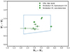 |
Fig. 9. MIR color–color plot for the GPs. The solid lines mark the regions used by Jarrett et al. (2011) to select AGNs. The GPs studied in Svoboda et al. (2019) and Kawamuro et al. (2019) are also included for comparison. |
3.2.2. Virial BH mass based on LAMOST optical spectra
Under the assumption that the broad-line region is virialized, the continuum luminosity is considered to represent the broad-line-region radius, and the width of the broad line to represent the virial velocity. The single-epoch spectra can be used to estimate the virial mass of the BHs (Shen et al. 2011). We used the following equations to estimate the virial BH mass:
In this work, we employed measurements based on the full width at half maximum of Hβ, and the coefficients are a = 0.910 and b = 0.50 (Vestergaard & Peterson 2006).
The virial mass of BHs can also be estimated from the broad Hα lines (Greene & Ho 2005). Greene & Ho (2005) and Shen et al. (2008, 2011) conducted multi-Gaussian fits to the broad Balmer lines and find the following correlation:
For virial BH mass estimators, the L5100 Å has a narrow dynamical range and suffers from host contamination in the low-luminosity range; therefore, we employed the following estimator based on Hα measurements:
where LHα is the Hα luminosity. The results are listed in Table 4.
BH masses of GPs.
3.2.3. MBH–M⋆ scaling relation
Scaling relations with the MBH can provide insights into the evolutionary history of BHs (Greene et al. 2020). The absorption features are not observable from the optical spectra; instead of the MBH–σ⋆ relation, we checked whether the GPs in this work follow the MBH–M⋆ scaling relation.
Greene et al. (2020) employed the form log MBH/M⊙ = α + βlog(M⋆/M0)+ϵ, obtaining fitted results of α = 7.56 ± 0.09, β = 1.39 ± 0.13, ϵ = 0.79 ± 0.05, and M0 = 3 × 10¹⁰ M⊙. We present the MBH relation of the GPs and this scaling relation in Fig. 10, where all the GPs comply with this MBH–M⋆ scaling relation.
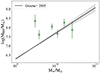 |
Fig. 10. MBH–M⋆ relation of the GPs. In the right panel, the solid line and the gray-shaded regions mark the scaling relation from Greene et al. (2020) and its scatter. |
3.3. Contributions from hot gas, hot ISM, and YSOs
According to the HMXB and hot gas scaling relations of Lehmer et al. (2022, their Eqs. (9)–(10)) and assuming that the hot gas only contributes to the soft energy band (0.5–2 keV), we have LX/(LHMXB + Lgas) > 3 for all sources. LX/SFR scaling relations of the hot ISM and YSOs (Winston et al. 2007; Mineo et al. 2012b) are L0.5#x2212;2 keV,ISM/SFR = 5.2 × 1038 (erg s−1/M⊙ yr−1) and L2x2212;10 keV,YSO/SFR = 1.7 × 1038 (erg s−1/M⊙ yr−1). Kawamuro et al. (2019) also modeled the contributions from the ISM and YSOs. As demonstrated in Fig. 6, hot ISM and YSOs are not enough to explain the excess X-ray luminosity of the GPs. Hot gas, hot ISM, and YSOs might contribute to the total X-ray luminosity of the GPs; however, these contributions are not enough to explain the observed LX/SFR.
4. Discussion
In this section we explore the elevated  values observed at lower metallicities.
4.1. The X-ray detection limit of the GPs
Based on the raw EPIC PN observation by the XMM-Newton X-ray observatory of the Lockman Hole field, Brunner et al. (2008) provide the sensitivity limit, which is defined as the faintest detectable source: 1.9 × 10⁻¹⁶ erg cm−2 s−1 in the 0.5 − 2.0 keV band, 9 × 10⁻¹⁶ erg cm−2 s−1 in the 2.0 − 10.0 keV band, and 1.8 × 10⁻¹⁵ erg cm−2 s−1 in the 5.0 − 10.0 keV band. The point source sensitivity of the Advanced CCD Imaging Spectrometer of the Chandra X-ray observatory is 4 × 10⁻¹⁵ erg cm−2 s−1 within 104 seconds in the energy range 0.4 − 6.0 keV6. The sensitivity of Swift/XRT is 8 × 10⁻¹⁴ erg cm−2 s−1 within 104 seconds in the energy range 0.2 − 10.0 keV7. Brunner et al. (2022) give the point-source flux limit of eFEDS to be 6.5 × 10⁻¹⁵ erg cm−2 s−1 in the 0.5 − 2.0 keV energy band.
Considering a GP located at z = 0.24, which is the lowest redshift where the [O III]λ5007 emission line lies within the r band, with a typical SFR of 10 M⊙ yr−1, we conducted the following calculations. Given the scaling relation from Mineo et al. (2012b), the X-ray flux from HMXBs in the 2 − 10 keV band in the rest frame is 1.4 × 10⁻¹⁶ erg cm−2 s−1. The X-ray flux from HMXBs derived from Lehmer et al. (2022) in the 0.5 − 8 keV band in the rest frame is 8.7 × 10⁻¹⁶ erg cm−2 s−1. Therefore, the X-ray luminosity from the HMXBs will be only barely detectable or not detectable by current X-ray facilities, depending on the exposure time of the instrument.
We employed Chandra observations to assess the proportion of GPs detected within the spatial coverage of Chandra. The LAMOST survey has identified 1887 unique GPs (Liu et al. 2022, 2023). Upon crossmatching them with the CSC using a search radius of 1 arcsec and a 1σ position error of 10 arcsec, we identified two detected sources (one true and one marginal) as well as 69 sources that are within the instrument’s limiting sensitivity. Consequently, the detection rate of GPs spatially covered by the instrument amounts to 1.4%.
Additionally, of the 69 sources with limiting sensitivity from Chandra, 26 are also covered by the GALEX and AllWISE surveys. Utilizing this multiwavelength data, we performed SED fitting with CIGALE as detailed in Sect. 2.2 but excluding the xray module. These sources are not detected in X-rays and typically have upper limits lower than the X-ray-selected GPs in this study, with LX/SFR values similar to those of local normal galaxies. As shown in Fig. 6, these non-detections, especially those with exposure times of less than 10 ks and larger off-axis angles from the image center, exhibit higher upper limits for LX/SFR. Increasing the depth of observations with longer exposure times could potentially allow us to detect more GPs with X-ray emissions and better constrain the upper limits for non-detections. Additionally, next-generation X-ray telescopes with reduced sensitivity limits would further these objectives.
4.2. The elevated  at low metallicities
There are potentially two sources contributing to the high LX/SFR in GPs: HMXBs and AGNs. Brorby et al. (2016) propose several hypotheses to explain the excess X-ray luminosity: (1) the presence of an additional X-ray flux source, possibly a hidden AGN, (2) a more substantial population of HMXBs in GPs compared to typical SFGs, and (3) a potential underestimation of the SFRs derived from optical spectral lines, IR luminosities, or UV luminosities. They favor the scenario involving a hidden AGN despite the scatter in X-ray measurements, which is yet to be corroborated by optical line diagnostics. The emitted X-rays cannot be solely accounted for by pure star formation, even with the inclusion of hot gas. A greater number of XRBs in the SFG with a steeper initial mass function might be plausible but cannot completely explain the scatter.
HMXBs typically consist of a BH or neutron star accreting material from a nearby massive (> 10 M⊙) stellar companion (Iben 1995; Bodaghee et al. 2012; Antoniou & Zezas 2016). Population synthesis models of XRBs explain the dependence of metallicity on  /SFR in two ways (Dray et al. 2006; Linden et al. 2010; Fragos et al. 2013a,b; Basu-Zych et al. 2013b): (1) weaker stellar winds in massive stars result in more mass that is retained and evolves into BHs, leading to higher LX(BH-HMXB)/SFR values compared to neutron star-HMXBs (Mapelli et al. 2009; Zampieri & Roberts 2009), and (2) reduced angular momentum loss from weaker stellar winds causes less orbital expansion, resulting in Roche-lobe overflow with higher accretion rates rather than Bondi-Hoyle wind accretion. In Fig. 6, the GPs predominantly occupy the high sSFR regime, with HMXBs dominating the XRB contributions.
We also incorporated the measurements of 11 low-redshift SFGs with high-quality constraints on X-ray emission from Chandra (Senchyna et al. 2020). These 11 galaxies show no signature of the existence of AGNs in the low-metallicity regime, 12 + log(O/H) 7.47 − 8.29. As demonstrated in Fig. 7, these low-redshift SFGs also follow the LX–SFR–metallicity relation, albeit with significant offsets. Senchyna et al. (2020) note that HMXBs are not the dominant source of the high ionization in the optical spectra and suggest that the solution may lie in revising stellar wind predictions, considering softer X-ray sources, or investigating very hot products of binary evolution at the low metallicity regime.
5. Summary
We studied a sample of six GPs with X-ray detections from XMM-Newton, Swift, Chandra, and eROSITA, as well as GPs from previous studies (Svoboda et al. 2019; Kawamuro et al. 2019). The SFRs, stellar masses, and ages of the GPs were determined using multiwavelength SED fitting via CIGALE. Metallicity assessments were based on optical spectra (Liu et al. 2022, 2023), with the BPT-classified AGNs measured using the Storchi-Bergmann et al. (1998) method. Furthermore, for the source with a relatively high S/N (J0035+0431), we conducted detailed X-ray spectral fitting using XMM-Newton data. We aimed to determine the origin of the X-ray luminosity and propose potential explanations.
In the context of the LX–SFR relation, GPs predominantly occupy the high sSFR regime (where HMXBs dominate), resulting in more LX compared to contributions solely from  . Furthermore, GPs exhibit a significant excess in LX in relation to the SFR and metallicity. According to MIR color–color criteria, six GPs fall within the AGN regime (Jarrett et al. 2011). Furthermore, based on the calculated MBH from LAMOST optical spectra, all GPs with AGNs from the MIR color–color plot comply with the MBH–M⋆ scaling relation (Greene et al. 2020). Contributions from XRBs, hot gas, hot ISM, and YSOs fail to fully explain the observed X-ray luminosity in GPs.
Although studies reveal elevated  values at lower metallicities (Dray et al. 2006; Linden et al. 2010; Fragos et al. 2013a,b; Basu-Zych et al. 2013b; Brorby et al. 2016), this is not enough to explain the excess of LX observed in these GPs. The X-ray excess observed in GPs is hypothesized to predominantly originate from the collective contribution of HMXBs and AGNs. The X-ray luminosities of the HMXBs of typical GPs are still above the detection limit of the current X-ray facilities. Further validation through X-ray spectra and high-resolution imaging is required.
Uncertainties remain regarding the sources of energetic photons responsible for heating and reionizing the early Universe. GPs, characterized by high SFRs and low metallicities, serve as local analogs of early high-z galaxies. Understanding the origin of the X-ray luminosity in GPs could help us uncover the energetic sources that ionize the high-z Universe.
The Large Sky Area Multi-Object Fiber Spectroscopic Telescope (LAMOST; Wang et al. 1996; Su & Cui 2004), which is located at the Xinglong Observatory, has an effective aperture of 4 m and can collect thousands of spectra at the same time (Cui et al. 2012).
Typically, Γ is 1.8 for AGNs, 1.56 for LMXBs, and 2.0 for HMXBs (Yang et al. 2020).
Kawamuro et al. (2019) used the Hα luminosity to calculate the SFR and obtain a higher result. For the sake of consistency, we used the measurements from Svoboda et al. (2019).
For GP1, whose X-ray spectrum is found to be significantly steeper, Svoboda et al. (2019) only constrain an upper limit in the 2–10 keV energy band.
Acknowledgments
This work is supported by the National Science Foundation of China (No. 12273075) and the National Key R&D Program of China (No. 2019YFA0405502). Guoshoujing Telescope (the Large Sky Area Multi-Object Fiber Spectroscopic Telescope, LAMOST) is a National Major Scientific Project built by the Chinese Academy of Sciences. Funding for the project has been provided by the National Development and Reform Commission. LAMOST is operated and managed by the National Astronomical Observatories, the Chinese Academy of Sciences. W. Zhang acknowledges support from the National Science Foundation of China (No. 12090041), the National Key R&D Program of China (No. 2021YFA1600401, 2021YFA1600400), and the Guangxi Natural Science Foundation (No. 2019GXNSFFA245008). S.L. thanks for the useful discussion with Meicun Hou on X-ray image reduction, Ru-Qiu Lin on green pea galaxies, and Hui-Mei Wang on flux calibration. This research has made use of data obtained from the 4XMM XMM-Newton Serendipitous Source Catalog compiled by the 10 institutes of the XMM-Newton Survey Science Centre selected by ESA. This research has made use of data obtained from the Chandra Source Catalog, provided by the Chandra X-ray Center (CXC) as part of the Chandra Data Archive. This work is based on data from eROSITA, the soft X-ray instrument aboard SRG, a joint Russian-German science mission supported by the Russian Space Agency (Roskosmos), in the interests of the Russian Academy of Sciences represented by its Space Research Institute (IKI), and the Deutsches Zentrum für Luft- und Raumfahrt (DLR). The SRG spacecraft was built by Lavochkin Association (NPOL) and its subcontractors and is operated by NPOL with support from the Max Planck Institute for Extraterrestrial Physics (MPE). The development and construction of the eROSITA X-ray instrument was led by MPE, with contributions from the Dr. Karl Remeis Observatory Bamberg & ECAP (FAU Erlangen-Nuernberg), the University of Hamburg Observatory, the Leibniz Institute for Astrophysics Potsdam (AIP), and the Institute for Astronomy and Astrophysics of the University of Tübingen, with the support of DLR and the Max Planck Society. The Argelander Institute for Astronomy of the University of Bonn and the Ludwig Maximilians Universität Munich also participated in the science preparation for eROSITA. The eROSITA data shown here were processed using the eSASS software system developed by the German eROSITA consortium.
References
- Aird, J., Coil, A. L., & Georgakakis, A. 2016, MNRAS, 465, 3390 [Google Scholar]
- Antoniou, V., & Zezas, A. 2016, MNRAS, 459, 528 [Google Scholar]
- Baldwin, J. A., Phillips, M. M., & Terlevich, R. 1981, PASP, 93, 5 [Google Scholar]
- Basu-Zych, A. R., Lehmer, B. D., Hornschemeier, A. E., et al. 2013a, ApJ, 762, 45 [NASA ADS] [CrossRef] [Google Scholar]
- Basu-Zych, A. R., Lehmer, B. D., Hornschemeier, A. E., et al. 2013b, ApJ, 774, 152 [NASA ADS] [CrossRef] [Google Scholar]
- Bianchi, L., Shiao, B., & Thilker, D. 2017, ApJS, 230, 24 [Google Scholar]
- Bodaghee, A., Tomsick, J. A., Rodriguez, J., & James, J. B. 2012, ApJ, 744, 108 [NASA ADS] [CrossRef] [Google Scholar]
- Boquien, M., Burgarella, D., Roehlly, Y., et al. 2019, A&A, 622, A103 [NASA ADS] [CrossRef] [EDP Sciences] [Google Scholar]
- Brorby, M., Kaaret, P., & Prestwich, A. 2014, MNRAS, 441, 2346 [NASA ADS] [CrossRef] [Google Scholar]
- Brorby, M., Kaaret, P., Prestwich, A., & Mirabel, I. F. 2016, MNRAS, 457, 4081 [NASA ADS] [CrossRef] [Google Scholar]
- Brunner, H., Cappelluti, N., Hasinger, G., et al. 2008, A&A, 479, 283 [NASA ADS] [CrossRef] [EDP Sciences] [Google Scholar]
- Brunner, H., Liu, T., Lamer, G., et al. 2022, A&A, 661, A1 [NASA ADS] [CrossRef] [EDP Sciences] [Google Scholar]
- Bruzual, G., & Charlot, S. 2003, MNRAS, 344, 1000 [NASA ADS] [CrossRef] [Google Scholar]
- Burgarella, D., Buat, V., & Iglesias-Páramo, J. 2005, MNRAS, 360, 1413 [NASA ADS] [CrossRef] [Google Scholar]
- Burrows, D. N., Hill, J. E., Nousek, J. A., et al. 2005, Space. Sci. Rev., 120, 165 [NASA ADS] [CrossRef] [Google Scholar]
- Cardamone, C., Schawinski, K., Sarzi, M., et al. 2009, MNRAS, 399, 1191 [NASA ADS] [CrossRef] [Google Scholar]
- Casey, C. M. 2012, MNRAS, 425, 3094 [Google Scholar]
- Chabrier, G. 2003, PASP, 115, 763 [Google Scholar]
- Cherinka, B., Andrews, B. H., Sánchez-Gallego, J., et al. 2019, AJ, 158, 74 [CrossRef] [Google Scholar]
- Colbert, E. J. M., Heckman, T. M., Ptak, A. F., Strickland, D. K., & Weaver, K. A. 2004, ApJ, 602, 231 [NASA ADS] [CrossRef] [Google Scholar]
- Cui, X.-Q., Zhao, Y.-H., Chu, Y.-Q., et al. 2012, RAA, 12, 1197 [NASA ADS] [Google Scholar]
- Douna, V. M., Pellizza, L. J., Mirabel, I. F., & Pedrosa, S. E. 2015, A&A, 579, A44 [NASA ADS] [CrossRef] [EDP Sciences] [Google Scholar]
- Dray, L. M., King, A. R., & Davies, M. B. 2006, MNRAS, 372, 31 [CrossRef] [Google Scholar]
- Durbala, A., Finn, R. A., Crone Odekon, M., et al. 2020, AJ, 160, 271 [NASA ADS] [CrossRef] [Google Scholar]
- Evans, I. N., Primini, F. A., Glotfelty, K. J., et al. 2010, ApJS, 189, 37 [NASA ADS] [CrossRef] [Google Scholar]
- Fornasini, F. M., Kriek, M., Sanders, R. L., et al. 2019, ApJ, 885, 65 [NASA ADS] [CrossRef] [Google Scholar]
- Fornasini, F. M., Civano, F., & Suh, H. 2020, MNRAS, 495, 771 [NASA ADS] [CrossRef] [Google Scholar]
- Fragos, T., Lehmer, B., Tremmel, M., et al. 2013a, ApJ, 764, 41 [NASA ADS] [CrossRef] [Google Scholar]
- Fragos, T., Lehmer, B. D., Naoz, S., Zezas, A., & Basu-Zych, A. 2013b, ApJ, 776, L31 [CrossRef] [Google Scholar]
- Freeman, P., Doe, S., & Siemiginowska, A. 2001, SPIE Conf. Ser., 4477, 76 [NASA ADS] [Google Scholar]
- Fu, Y. 2021, QSOFITMORE: A Python Package for Fitting UV-optical Spectra of Quasars, https://doi.org/10.5281/zenodo.4893646 [Google Scholar]
- Gilfanov, M., Grimm, H. J., & Sunyaev, R. 2004a, MNRAS, 347, L57 [NASA ADS] [CrossRef] [Google Scholar]
- Gilfanov, M., Grimm, H. J., & Sunyaev, R. 2004b, MNRAS, 351, 1365 [NASA ADS] [CrossRef] [Google Scholar]
- Greene, J. E., & Ho, L. C. 2005, ApJ, 630, 122 [NASA ADS] [CrossRef] [Google Scholar]
- Greene, J. E., Strader, J., & Ho, L. C. 2020, ARA&A, 58, 257 [Google Scholar]
- Grimes, J. P., Heckman, T., Strickland, D., et al. 2007, ApJ, 668, 891 [NASA ADS] [CrossRef] [Google Scholar]
- Grimm, H. J., Gilfanov, M., & Sunyaev, R. 2003, MNRAS, 339, 793 [Google Scholar]
- Hao, C.-N., Kennicutt, R. C., Johnson, B. D., et al. 2011, ApJ, 741, 124 [Google Scholar]
- Harish, S., Malhotra, S., Rhoads, J. E., et al. 2023, ApJ, 945, 157 [NASA ADS] [CrossRef] [Google Scholar]
- Hunter, D. A., Elmegreen, B. G., & Ludka, B. C. 2010, AJ, 139, 447 [NASA ADS] [CrossRef] [Google Scholar]
- Iben, I., Tutukov, A. V., & Yungelson, L. R. 1995, ApJS, 100, 217 [NASA ADS] [CrossRef] [Google Scholar]
- Iwasawa, K., Sanders, D. B., Evans, A. S., et al. 2009, ApJ, 695, L103 [NASA ADS] [CrossRef] [Google Scholar]
- Jarrett, T. H., Cohen, M., Masci, F., et al. 2011, ApJ, 735, 112 [Google Scholar]
- Jiang, T., Malhotra, S., Rhoads, J. E., & Yang, H. 2019, ApJ, 872, 145 [NASA ADS] [CrossRef] [Google Scholar]
- Kauffmann, G., Heckman, T. M., Tremonti, C., et al. 2003, MNRAS, 346, 1055 [Google Scholar]
- Kawamuro, T., Ueda, Y., Ichikawa, K., et al. 2019, ApJ, 881, 48 [NASA ADS] [CrossRef] [Google Scholar]
- Kennicutt, R. C., & Evans, N. J. 2012, ARA&A, 50, 531 [NASA ADS] [CrossRef] [Google Scholar]
- Kewley, L. J., Dopita, M. A., Sutherland, R. S., Heisler, C. A., & Trevena, J. 2001, ApJ, 556, 121 [Google Scholar]
- Kewley, L. J., Groves, B., Kauffmann, G., & Heckman, T. 2006, MNRAS, 372, 961 [Google Scholar]
- Kormendy, J., & Ho, L. C. 2013, ARA&A, 51, 511 [Google Scholar]
- Kormendy, J., & Richstone, D. 1995, ARA&A, 33, 581 [Google Scholar]
- Lehmer, B. D., Alexander, D. M., Bauer, F. E., et al. 2010, ApJ, 724, 559 [Google Scholar]
- Lehmer, B. D., Basu-Zych, A. R., Mineo, S., et al. 2016, ApJ, 825, 7 [Google Scholar]
- Lehmer, B. D., Eufrasio, R. T., Tzanavaris, P., et al. 2019, ApJS, 243, 3 [NASA ADS] [CrossRef] [Google Scholar]
- Lehmer, B. D., Eufrasio, R. T., Basu-Zych, A., et al. 2021, ApJ, 907, 17 [NASA ADS] [CrossRef] [Google Scholar]
- Lehmer, B. D., Eufrasio, R. T., Basu-Zych, A., et al. 2022, ApJ, 930, 135 [NASA ADS] [CrossRef] [Google Scholar]
- Linden, T., Kalogera, V., Sepinsky, J. F., et al. 2010, ApJ, 725, 1984 [Google Scholar]
- Liu, S., Luo, A. L., Yang, H., et al. 2022, ApJ, 927, 57 [NASA ADS] [CrossRef] [Google Scholar]
- Liu, S., Luo, A. L., Zhang, W., et al. 2023, ApJS, 267, 16 [NASA ADS] [CrossRef] [Google Scholar]
- Madau, P., & Fragos, T. 2017, ApJ, 840, 39 [Google Scholar]
- Mapelli, M., Colpi, M., & Zampieri, L. 2009, MNRAS, 395, L71 [NASA ADS] [CrossRef] [Google Scholar]
- Mineo, S., Gilfanov, M., & Sunyaev, R. 2012a, MNRAS, 419, 2095 [Google Scholar]
- Mineo, S., Gilfanov, M., & Sunyaev, R. 2012b, MNRAS, 426, 1870 [NASA ADS] [CrossRef] [Google Scholar]
- Persic, M., & Rephaeli, Y. 2007, A&A, 463, 481 [NASA ADS] [CrossRef] [EDP Sciences] [Google Scholar]
- Persic, M., Rephaeli, Y., Braito, V., et al. 2004, A&A, 419, 849 [NASA ADS] [CrossRef] [EDP Sciences] [Google Scholar]
- Pettini, M., & Pagel, B. E. J. 2004, MNRAS, 348, L59 [NASA ADS] [CrossRef] [Google Scholar]
- Planck Collaboration XI. 2014, A&A, 571, A11 [NASA ADS] [CrossRef] [EDP Sciences] [Google Scholar]
- Ranalli, P., Comastri, A., & Setti, G. 2003, A&A, 399, 39 [NASA ADS] [CrossRef] [EDP Sciences] [Google Scholar]
- Schlegel, D. J., Finkbeiner, D. P., & Davis, M. 1998, ApJ, 500, 525 [Google Scholar]
- Senchyna, P., Stark, D. P., Mirocha, J., et al. 2020, MNRAS, 494, 941 [CrossRef] [Google Scholar]
- Shen, J., Vanden Berk, D. E., Schneider, D. P., & Hall, P. B. 2008, AJ, 135, 928 [NASA ADS] [CrossRef] [Google Scholar]
- Shen, Y., Richards, G. T., Strauss, M. A., et al. 2011, ApJS, 194, 45 [Google Scholar]
- Stalevski, M., Fritz, J., Baes, M., Nakos, T., & Popović, L. Č. 2012, MNRAS, 420, 2756 [Google Scholar]
- Stalevski, M., Ricci, C., Ueda, Y., et al. 2016, MNRAS, 458, 2288 [Google Scholar]
- Storchi-Bergmann, T., Schmitt, H. R., Calzetti, D., & Kinney, A. L. 1998, AJ, 115, 909 [NASA ADS] [CrossRef] [Google Scholar]
- Su, D.-Q., & Cui, X.-Q. 2004, Chin. J. Astron. Astrophys, 4, 1 [NASA ADS] [CrossRef] [Google Scholar]
- Svoboda, J., Douna, V., Orlitová, I., & Ehle, M. 2019, ApJ, 880, 144 [NASA ADS] [CrossRef] [Google Scholar]
- Traulsen, I., Schwope, A. D., Lamer, G., et al. 2020, A&A, 641, A137 [NASA ADS] [CrossRef] [EDP Sciences] [Google Scholar]
- Veilleux, S., & Osterbrock, D. E. 1987, ApJS, 63, 295 [Google Scholar]
- Vestergaard, M., & Peterson, B. M. 2006, ApJ, 641, 689 [Google Scholar]
- Wang, S.-G., Su, D.-Q., Chu, Y.-Q., Cui, X., & Wang, Y.-N. 1996, Appl. Opt., 35, 5155 [NASA ADS] [CrossRef] [Google Scholar]
- Webb, N. A., Coriat, M., Traulsen, I., et al. 2020, A&A, 641, A136 [NASA ADS] [CrossRef] [EDP Sciences] [Google Scholar]
- Winston, E., Megeath, S. T., Wolk, S. J., et al. 2007, ApJ, 669, 493 [NASA ADS] [CrossRef] [Google Scholar]
- Wright, E. L., Eisenhardt, P. R. M., Mainzer, A. K., et al. 2010, AJ, 140, 1868 [Google Scholar]
- Wright, E. L., Eisenhardt, P. R. M., Mainzer, A. K., et al. 2019, AllWISE Source Catalog (IPAC) [Google Scholar]
- Yang, G., Boquien, M., Buat, V., et al. 2020, MNRAS, 491, 740 [Google Scholar]
- Yang, G., Boquien, M., Brandt, W. N., et al. 2022, ApJ, 927, 192 [NASA ADS] [CrossRef] [Google Scholar]
- Zampieri, L., & Roberts, T. P. 2009, MNRAS, 400, 677 [NASA ADS] [CrossRef] [Google Scholar]
Appendix A: CIGALE SED fitting result
We show the remaining CIGALE SED fitting results in Fig. A.1.
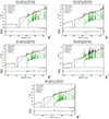 |
Fig. A.1. CIGALE SED fitting result for the rest of the sources. |
Appendix B: Fitting result from QSOFITMORE
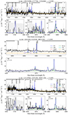 |
Fig. B.1. Spectral fitting result from QSOFITMORE. In the upper panels of the subplots, black lines denote the total de-reddened spectra (corrected for Galactic extinction from Planck Collaboration XI (2014)), yellow lines denote the continua, cyan lines depict the Fe II templates, blue lines indicate the whole emission lines, red lines represent the broad-line components, green lines denote the narrow-line components, and the gray shaded area mark the error region of the spectra. The lower panels demonstrate the zoomed-in fitting results of the different emission lines. |
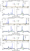 |
Fig. B.1. continued. |
All Tables
All Figures
|
Fig. 1. Two GPs with X-ray detections from XMM-Newton (J1330-0043 and J0035+0431). Left panels: SDSS and XMM-Newton image cutouts. Right panels: LAMOST spectra. The black lines mark flux-calibrated spectra, the orange curves the spectra smoothed with a Gaussian kernel standard deviation of 3 pixels, and the gray-shaded regions the flux error. |
| In the text | |
|
Fig. 2. GPs with X-ray detection from Swift (J0205+1504 and J0227+2355; top two rows), the GP with X-ray detection from Chandra (J1605+4405; third row), and the GP with X-ray detection from eROSITA (J0906+0242; bottom row). Left panels: SDSS, Swift, and Chandra image cutouts. Right panels: LAMOST spectra. The black lines mark the flux-calibrated spectrum, the orange curves the spectrum smoothed with a kernel of 3, and the gray-shaded regions the flux error. |
| In the text | |
|
Fig. 3. CIGALE SED fitting result for source J0035+0431. |
| In the text | |
|
Fig. 4. BPT diagram of the GPs with spectral coverage. The plotting routine is based on that from Cherinka et al. (2019). |
| In the text | |
|
Fig. 5. X-ray flux from different energy bands for source J0035+0431, and the fitted spectra from XMM-Newton. |
| In the text | |
|
Fig. 6. Relations of the rest-frame X-ray luminosity in the 2–10 keV (left panel) and 0.5–8 keV energy bands (right panel) per SFR vs. sSFR. The green circles mark the GP measurements. Different LX–SFR relations in the form of Eq. (2) are marked in the left panel (Lehmer et al. 2010; Mineo et al. 2012b) and the right panel (Lehmer et al. 2019, 2022); the shaded regions mark the 1σ scatter. The gray downward pointing arrows indicate the upper limits of GPs with only limiting sensitivities from Chandra (see Sect. 4.1 for a discussion). The arrow size corresponds to the exposure time, with larger arrows indicating longer exposure times. The grayscale represents the source’s off-axis angle from the image center, with lighter shades indicating larger off-axis angles. |
| In the text | |
|
Fig. 7. LX–SFR–metallicity relation of the GPs. Green open circles with error bars represent the GPs in this study. The solid line denotes the best-fit LX–SFR–metallicity relation from Brorby et al. (2016), with dashed lines indicating a dispersion of σ = 0.34 dex. Red circles represent SFGs from Douna et al. (2015), and magenta squares represent LBAs from Brorby et al. (2016). Orange open circles indicate seven detections from Chandra observations, while orange triangles denote the four upper limits for low-redshift SFGs (Senchyna et al. 2020). |
| In the text | |
|
Fig. 8. LX/SFR–metallicity relation of the GPs. The green open circles with error bars mark the GPs in this work. Scaling relations from Fragos et al. (2013b), Madau & Fragos (2017), and Lehmer et al. (2021) are marked with different lines. The brown diamonds mark the LBGs from Basu-Zych et al. (2013b). |
| In the text | |
|
Fig. 9. MIR color–color plot for the GPs. The solid lines mark the regions used by Jarrett et al. (2011) to select AGNs. The GPs studied in Svoboda et al. (2019) and Kawamuro et al. (2019) are also included for comparison. |
| In the text | |
|
Fig. 10. MBH–M⋆ relation of the GPs. In the right panel, the solid line and the gray-shaded regions mark the scaling relation from Greene et al. (2020) and its scatter. |
| In the text | |
|
Fig. A.1. CIGALE SED fitting result for the rest of the sources. |
| In the text | |
|
Fig. B.1. Spectral fitting result from QSOFITMORE. In the upper panels of the subplots, black lines denote the total de-reddened spectra (corrected for Galactic extinction from Planck Collaboration XI (2014)), yellow lines denote the continua, cyan lines depict the Fe II templates, blue lines indicate the whole emission lines, red lines represent the broad-line components, green lines denote the narrow-line components, and the gray shaded area mark the error region of the spectra. The lower panels demonstrate the zoomed-in fitting results of the different emission lines. |
| In the text | |
|
Fig. B.1. continued. |
| In the text | |
Current usage metrics show cumulative count of Article Views (full-text article views including HTML views, PDF and ePub downloads, according to the available data) and Abstracts Views on Vision4Press platform.
Data correspond to usage on the plateform after 2015. The current usage metrics is available 48-96 hours after online publication and is updated daily on week days.
Initial download of the metrics may take a while.