| Issue |
A&A
Volume 693, January 2025
|
|
|---|---|---|
| Article Number | A254 | |
| Number of page(s) | 15 | |
| Section | Extragalactic astronomy | |
| DOI | https://doi.org/10.1051/0004-6361/202452735 | |
| Published online | 23 January 2025 | |
Physical characterization of the FeLoBAL outflow in SDSS J0932+0840: Analysis of VLT/UVES observations
1
Department of Physics, Virginia Tech, Blacksburg, VA 24061, USA
2
Department of Physics, Western Michigan University, 1120 Everett Tower, Kalamazoo, MI 49008-5252, USA
3
Department of Astronomy, University of Michigan, Ann Arbor, MI 48109, USA
⋆ Corresponding author; This email address is being protected from spambots. You need JavaScript enabled to view it.
Received:
24
October
2024
Accepted:
9
December
2024
Abstract
Context. The study of quasar outflows is essential for understanding the connection between active galactic nuclei (AGN) and their host galaxies. We analyzed the VLT/UVES spectrum of quasar SDSS J0932+0840 and identified several narrow and broad outflow components in absorption, with multiple ionization species including Fe II. This places it among the rare class of outflows known as iron low-ionization broad absorption line outflows (FeLoBALs).
Aims. We studied one of the outflow components to determine its physical characteristics by determining the total hydrogen column density, the ionization parameter, and the hydrogen number density. Through these parameters, we obtained the distance of the outflow from the central source, its mass outflow rate, and its kinetic luminosity, and we constrained the contribution of the outflow to the AGN feedback.
Methods. We obtained the ionic column densities from the absorption troughs in the spectrum and used photoionization modeling to extract the physical parameters of the outflow, including the total hydrogen column density and ionization parameter. The relative population of the observed excited states of Fe II was used to model the hydrogen number density of the outflow.
Results. We used the Fe II excited states to model the electron number density (ne) and hydrogen number density (nH) independently and obtained ne ≃ 103.4 cm−3 and nH ≃ 104.8 cm−3. Our analysis of the physical structure of the cloud shows that these two results are consistent with each other. This places the outflow system at a distance of 0.7−0.4+0.9 kpc from the central source, with a mass flow rate (Ṁ) of 43−26+65 M⊙ yr−1 and a kinetic luminosity (Ėk) of 0.7−0.4+1.1 × 1043 erg s−1. This is 0.5−0.3+0.7 × 10⁻⁴ of the Eddington luminosity (LEdd) of the quasar, and we thus conclude that this outflow is not powerful enough to contribute significantly toward AGN feedback.
Key words: galaxies: active / galaxies: evolution / galaxies: kinematics and dynamics / quasars: absorption lines / quasars: individual: SDSS J093224.48-084008.0
© The Authors 2025
 Open Access article, published by EDP Sciences, under the terms of the Creative Commons Attribution License (https://creativecommons.org/licenses/by/4.0), which permits unrestricted use, distribution, and reproduction in any medium, provided the original work is properly cited.
This article is published in open access under the Subscribe to Open model. This email address is being protected from spambots. You need JavaScript enabled to view it. to support open access publication.
1. Introduction
Quasar outflows are detected as blueshifted absorption troughs relative to the systemic redshift of the active galactic nuclei (AGN). They are observed ubiquitously and are invoked as the primary mechanism in the quasar mode of AGN feedback. They may play an important role in the evolution of the supermassive black hole (SMBH; e.g., Silk & Rees 1998; Begelman & Nath 2005; Hopkins et al. 2009; Liao et al. 2024), in that of the host galaxy (e.g., Di Matteo et al. 2005; Ostriker et al. 2010; Choi et al. 2017; Cochrane et al. 2023), in the enrichment of the intergalactic medium (e.g., Moll et al. 2007; Fabjan et al. 2010; Ciotti et al. 2022), and in cooling flows in clusters of galaxies (e.g., Begelman & Ruszkowski 2005; Brüggen & Scannapieco 2009; Hopkins et al. 2016; Weinberger et al. 2023).
Based on the width of the detected absorption lines (defined as continuous absorption with a normalized flux < 0.9), quasar outflows are commonly classified into one of the three following categories: Broad absorption lines (BALs) are defined as having a velocity width of Δv≳ 2000 km s−1, and they are found in ∼20% of the quasar spectra (Weymann et al. 1991; Hewett & Foltz 2003; Reichard et al. 2003; Knigge et al. 2008), mini-BALs have velocity widths of 500 ≲Δv≲ 2000 km s−1 and an incidence rate of ∼10% (Hamann & Sabra 2004; Hidalgo et al. 2012; Moravec et al. 2017; Chen et al. 2021), and finally, narrow absorption lines (NALs) with a velocity width of Δv≲ 500 km s−1 are the most common features and are detected in ∼60% of the quasar spectra (Vestergaard 2003; Ganguly & Brotherton 2008; Stone & Richards 2019).
Broad absorption line quasar outflows (BALQSO) have further been classified into three categories based on the ionization state of the observed absorption lines in their spectra (Hall et al. 2002). High-ionization BALQSOs (HiBALs) only show absorption from high-ionization species, such as C IV, Si IV, N V, and O VI, and they are most common and observed in all BALQSOs (Voit et al. 1993; Dai et al. 2012). Low-ionization BALQSOs (LoBALs) show absorption lines from the high-ionization species, but are also accompanied by lower-ionization species such as Mg II, C II, and Al III. They are observed in ∼10% of the BALQSOs (Weymann et al. 1991; Trump et al. 2006). The rarest class are iron low-ionization BALQSOs (FeLoBALs), which show absorption from both high- and low-ionization species along with Fe II or Fe III. They make up just ∼0.3% of the quasar population (Trump et al. 2006).
Theoretically, these classifications for quasar outflows are understood through two different models. In the context of an orientation-based model, BALQSOs are observed as a result of the intersection of our line of sight with outflowing gas that is launched from a narrow range of radii on the accretion disk (Murray et al. 1995; Elvis 2000). The different ionization subclasses then relate to the column density of the material they encounter, with HiBALS having the smallest column and FeLoBALs having the largest, extending beyond the H II region (Arav et al. 2001a; Korista et al. 2008; Lucy et al. 2014). The opening angle for this line of sight would be small (Green et al. 2001; Gallagher et al. 2006; Morabito et al. 2011) and thus explains the rarity of FeLoBALs. An alternative evolutionary model suggests that FeLoBALs might represent a short-lived phase in which a young quasar is observed in the process of breaking through a cocoon of enveloping dust and gas (Voit et al. 1993).
The FeLoBALs usually show a plethora of absorption troughs from ground-state and various excited-state transitions, which makes them an excellent diagnostic of the physical state of the outflowing gas. Arav et al. (2001b) and de Kool et al. (2001, 2002a,b) presented some of the first detailed photoionization analyses of FeLoBAL quasars based on Keck High Resolution Echelle Spectrometer (HIRES) spectra and obtained constraints on the temperature, the ionization parameter (UH), the electron number density (ne), and the distance from the emission source (R) for the outflows. Korista et al. (2008), Arav et al. (2008), Moe et al. (2009), Dunn et al. (2010), and Bautista et al. (2010) used high-resolution spectra with a high signal-to-noise ratio from the Very Large Telescope (VLT) and the Astrophysical Research Consortium telescope (ARC). This allowed them to improve the accuracy of the column density and number density measurements and obtain mass flux and kinetic luminosity for some outflows, thus constraining the extent of their contribution to AGN feedback processes. Leighly et al. (2018) introduced the novel spectral synthesis procedure SimBAL, which has led to an impressive increase in the number of FeLoBALs that were subjected to a detailed spectral analysis. Choi et al. (2022a) presented a SimBAL analysis of 50 low-redshift FeLoBAL quasars that covered a wide range in the parameter space for UH, ne, and R, and introduced a new class of loitering FeLoBAL outflows. Choi et al. (2022b) and Leighly et al. (2022) extended this analysis further to the geometry of the outflows and the optical line emission properties for the host quasars. Other recent studies of individual quasar outflows have led to the discovery of increasingly interesting properties and phenomenon: Choi et al. (2020) discovered a remarkably powerful FeLoBAL outflow with the highest observed velocity and kinetic luminosity so far, Xu et al. (2021) found differences in the physical conditions for the Fe II and Fe III formation in Q0059–2735, Byun et al. (2022a) found the farthest known mini-BAL outflow system at ∼67 kpc and along with Walker et al. (2022), an extremely high mass outflow rate that might contribute significantly to AGN feedback processes.
We present a study of the Ultraviolet and Visual Echelle Spectrograph (UVES) spectrum of the quasar SDSS J093224.48+084008.0 (hereafter, J0932+0840), obtained with the VLT. Section 2 describes the observation and how we obtained the data for our analysis. In Sect. 3 we analyze the spectrum to obtain the column densities of the observed troughs, along with the photoionization modeling of the outflow. Section 4 discusses our diagnostics for the outflow electron and hydrogen number densities based on the population of the observed excited states. Section 5 presents the energetics of the outflow. Section 6 discusses the observed variability between the different epochs, along with a reevaluation of properties from a few previous FeLoBAL studies. Finally, we summarize and conclude the paper in Sect. 7. Throughout the paper, we adopt a standard ΛCDM cosmology with h = 0.677, Ωm = 0.310 and ΩΛ = 0.690 (Planck Collaboration VI 2020).
2. Data overview
2.1. Observation and data acquisition
J0932+0840 (J2000: RA = 09:32:24.48; Dec: +08:40:08.0) was observed with VLT/UVES on 30 April 2008 with a total exposure time of 28.1 ks as part of program 081.B-0285 (PI: Benn). The data cover a spectral range of 3758–10 250 Å, with a resolution of R ≈ 48 000 and an average signal-to-noise ratio S/N ≈ 30 per resolution element. The data were then reduced and normalized by Murphy et al. (2019) as part of the first data release (DR1) of the UVES Spectral Quasar Absorption Database (SQUAD). Figure 3 shows the obtained normalized data.
J0932+0840 was also observed on two occasions (20 December 2003 and 26 January 2012) as part of the Sloan Digital Sky Survey (SDSS). While our primary analysis is based on the SQUAD data with their higher resolution and S/N, it lacks information about any emission features as it is normalized. We therefore used the SDSS spectrum (Fig. 1) to (i) obtain the redshfit of the quasar (Sect. 2.2), (ii) scale the flux of our spectral energy distribution (SED) to obtain the bolometric luminosity (Sect. 5.1), and (iii) obtain the black hole mass (Sect. 5.2).
 |
Fig. 1. Non-normalized SDSS spectra of J0932+0840 (2012 epoch). The flux density (Fλ) is shown in black, and the error is plotted in gray. |
2.2. Redshift determination
The second epoch of the SDSS observation (Fig. 1) covers the Mg IIλλ 2796.35, 2803.53 emission feature. This feature can be used to obtain the redshfit of the quasar. We first modeled the underlying continuum emission with a power law and then modeled the Mg II emission feature with a single Gaussian. The result of this fit is shown in Fig. 2. This led to a redshift of z = 2.308 ± 0.001. This is close to the redshift estimate obtained by Yi et al. (2019) (z = 2.300) in their study of 134 Mg II broad absorption line (BAL) quasars including J0932+0840. We note, however, that these redshift values disagree with the value determined by Hewett & Foltz (2003) (z = 2.341231 ± 0.001884). These authors determined this value by modeling the 1900 blend, which includes Al III 1857 (λλ 1854.72, 1862.78), SiIII] 1892 (λ 1892.03), and the CIII] 1909 (λ 1908.73) emission lines in the first epoch of SDSS observation, as it does not cover the Mg II emission feature. As this blend includes multiple emission features of similar strengths, it is more prone to uncertainty than the fit obtained for Mg II, and we therefore used z = 2.308 for our analysis.
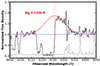 |
Fig. 2. Gaussian model fit for the Mg II 2799 emission feature (shown in red). Due to high absorption, the data points for the fit were selected manually. The dashed red line marks the centroid of the best-fit model we used to determine the redshift of the quasar. The dashed blue line shows the continuum level. The error on the flux is shown in gray. |
3. Spectral analysis
3.1. Identifying outflow systems
The UVES spectrum of J0932+0840 shows a large number of absorption systems ranging in velocities from −500 to −5000 km s−1. The lowest-velocity systems (∼−500, −700 and −850 km s−1) are narrow absorption lines (Δv∼ 100 km s−1) and are observed in most species, including low- and high-ionization lines. The higher-velocity systems (∼−1300, −4200 and −5000 km s−1) are much broader (with Δv≳ 2000 km s−1, and thus classified as BALs), and are only seen in a few species such as Si II, C II, Mg II, Al III, Si IV, and C IV (the latter is only covered in the SDSS spectrum). The focus of this paper is on the system with velocity ∼−700 km s−1 (hereafter S2) as it shows absorption from the most species and is thus rich in diagnostics.
3.2. Column density determination
In order to constrain the physical characteristics of an outflow system, it is important to obtain the column densities of the observed ionic species. For a given ionic transition with a rest wavelength λ (in Angstroms) and oscillator strength f, the column density Nion is obtained using (Savage & Sembach 1991)
![Mathematical equation: $$ \begin{aligned} N_{\rm ion} = \frac{m_e c}{\pi e^2 f \lambda } \int \tau (v)\,\text{ d}v = \frac{3.8 \times 10^{14}}{f \lambda } \int \tau (v) \,\text{ d}v\,[\mathrm{cm}^{-2}], \end{aligned} $$](/articles/aa/full_html/2025/01/aa52735-24/aa52735-24-eq5.gif) (1)
(1)
where me is the electron mass, c is the speed of light, e is the elementary charge, and τ(v) is the optical depth profile for the transition, which is based on the choice of the absorber model. The simplest model, known as the apparent optical depth (AOD) model, assumes a homogeneous outflow that completely covers the source. In this case, the normalized intensity profile I(v) is then simply related to τ(v) as
 (2)
(2)
This model does not account for partial line-of-sight (LOS) covering and saturation effects in line centers and can thus underestimate the column densities. For saturated troughs, only lower limits to the column densities can therefore be obtained with the AOD model. In the case of J0932+0840, however, we detected several weak transitions that have low oscillator strength values. These troughs are much shallower than the other deeper troughs from the same ion and can thus be considered unsaturated. We therefore regarded the derived column densities for these transitions as actual measurements.
When two or more lines from the same lower-energy level were detected for an ion, we employed a more physical inhomogeneous absorber model in which the gas distribution is approximated with a power law (de Kool et al. 2002c; Arav et al. 2005). The optical depth profile within the outflow is then described as
 (3)
(3)
where x is the spatial dimension across our LOS, and a is the power law index. Then, given two or more intensity profiles, we solved for τmax and a simultaneously.
The unsaturated absorption troughs of Fe II cover a velocity range −820≲ v ≲ − 600 km s−1 and were modeled by a Gaussian profile based on the Fe II* 1278 Å trough. The corresponding best-fit profile was scaled to match the other Fe II troughs, and the final fits are shown in Fig. 4. Except for the 7955 and 8680 cm−1 levels, all other troughs appear to be unsaturated, and therefore, their AOD column densities were taken as measurements. We also detected multiple unsaturated transitions from the 385, 668, 863, and 1873 cm−1 levels and therefore applied the power-law (PL) model to obtain their column densities. We find that for these transitions, the Nion values derived from the PL method are similar to the AOD model and therefore lend credibility to the AOD column densities derived for other species. We repeated this analysis for the other observed troughs in the spectrum and report their column densities in Table 1. The reported error bars for the column density measurements include a 20% relative error added in quadrature to account for systemic uncertainties, following the method described by Xu et al. (2018).
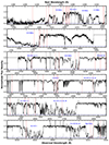 |
Fig. 3. Normalized UVES spectrum of J0932-0840. Important features and multiplets are marked in blue, and the identified absorption troughs from the primary outflow system at v ≈ −720 km s−1 are marked with dashed red lines. The zero flux level is shown by the dashed blue lines. The dashed black lines mark troughs from an intervening system at z = 1.28. |
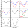 |
Fig. 4. Identified Fe II troughs for outflow system S2. The histograms show the VLT/UVES spectra in velocity space, and the corresponding dashed curves show the modeled Gaussian for the absorption. The model is based on the 1278 Å transition, and its template with fixed centroid and width was scaled to match the depth of all other troughs. The lower-energy level of the transition and the wavelengths are given for each panel. |
Absorption lines identified in the VLT spectrum of SDSS J0932+0840 and their measured column densities.
3.3. Calculating the oscillator strength for Fe II transitions
As mentioned above, a special feature of the VLT spectrum of J0932+0840 is the detection of unsaturated troughs that correspond to transitions with very weak oscillator strengths. The Fe II 1901.78 ground-state transition is the weakest of these transitions, with a theoretically determined oscillator strength of 6.25 × 10⁻⁵ (Kurucz & Bell 1995), and is thus rarely observed. The only other detection in a quasar spectrum was reported by Byun et al. (2024). This rarity means, however, that the oscillator strength value for the transition remains poorly constrained by observations and is prone to uncertainties. As this transition is of central importance in our work (see Sect. 4), we performed our own calculations to obtain an estimate for the oscillator strength along with its uncertainties.
We modeled the Fe II atomic system and computed gf values for dipole bound-bound transitions using the computer code AUTOSTRUCTURE (Badnell 2011). AUTOSTRUCTURE solves the Breit–Pauli Schrödinger equation with a scaled Thomas–Fermi–Dirac-Amaldi (TFDA) central-field potential to generate orthonormal atomic orbitals. Configuration interaction (CI) atomic state functions are built using these orbitals. The scaling factors of the potential for each orbital are generally optimized in a multiconfiguration variational procedure minimizing a sum over LS term energies or a weighted average of LS term energies. This optimization can be made on nonrelativistic LS calculations or with one-body relativistic operators.
Two types of corrections are enabled by the code after optimizing the orbitals. Perturbative term energy correction (TEC) can be applied to the multi-electronic Hamiltonian, which adjusts theoretical LS term energies closer to the centers of gravity of the available experimental multiplets. Level energy corrections (LEC) can also be applied to shift the theoretical energy levels to reproduce matching level energy separations when computing f values and transition probabilities.
For large calculations such as ours, AUTOSTRUCTURE was run from our own PYTHON wrapper for the semi-automatic generation of input files with large configuration expansions, analysis of output files, comparisons of energies and radiative data, and TEC and LEC corrections. We carried out numerous calculations for the Fe II system, systematically added configurations to the CI expansion, and fully optimized the orbitals with every expansion. The aim was to include within the computational limits all configurations that contribute to improving the energies of the terms belonging to the 3d64s, 3d7, 3d54s2, 3d64p, and 3d54s4p configurations relative to the experimental values, as well as the convergence of the gf values for the transitions of interest. The energies of the 3d7 a 4F levels relative to levels of the 3d64s a 6D ground term are particulaarly challenging and important because all observed transitions in this work arise from them.
Our final expansion included 11 orbitals (1s, 2s, 2p 3s, 3p, 3d, 4s, 4p, 4d, 5s, 5p) in 61 configurations with 1s and 2s closed-core orbitals: 3d7, 3d6nl (n = 4 − 5, l = 0–2), 3d5nln′l′ (n = 4–5, l = 0–2, n′ = 4–5, l′ = 0–2), 3p53d8, 3p53d7nl (n = 4–5, l = 0–2), 3p53d64snl (n = 4–5, l = 0–2), 3p43d9, 3p43d8nl (n = 4–5, l = 0–2), 3p43d7nl2 (n = 4–5, l = 0–2), 3s3p63d8, 3s3p63d7nl (n = 4–5, l = 0–2), 3s3p63d64s2, 2p53s23p63d8, 2p53s23p63d7nl (n = 4–5, l = 0–2), 2p53s23p63d64s2, 2p63p63d9, 2p63p63d84s, 2p63p63d74s2, 2p63p63d74s4p, 2p43s23p63d9, 2p43s23p63d84s, 2p43s23p63d74l2 (l = 0–2).
An important issue to highlight with these calculations is that when an acceptable level of converse was achieved in terms of the predicted energies, a further slight optimization of the 3d and 4s orbitals had to be performed manually on fine-structure energy levels rather than the numerical optimization based on LS terms incorporated in AUTOSTRUCTURE for the correct ordering and energy separations between the 3d7 a 4F and 3d64s a 6D levels. The energy separation between these is comparable to the magnitude of the two-body relativistic corrections, hence optimizations in LS-coupling of these terms is unphysical and becomes severely disrupted in final jj-coupling computations. Moreover, the relativistic jj-coupling correction on level energies is highly nonlineal upon initial LS term energies. Because of the magnitude of two-body energy corrections on levels of the 3d7 a 4F and 3d64s a 6D, no perturbative TEC can be employed. The orbitals must instead be optimized by hand to obtain accurate level energies, and simple LEC was then applied for the final computation of gf values.
Our calculation resulted into 669 energy levels from the five configurations listed above. These levels yield nearly 40 000 dipole-allowed transitions and over 100 000 dipole-forbidden transitions. This extensive dataset enables the proper identification of the troughs observed in our experiment, many of which were not found in previously published tabulations of Fe II gf values. We recall that the Fe II troughs identified in the VLT/X-Shooter spectrum of J0932+0840 are intrinsically weak transitions, and their gf values therefore carry a significant uncertainty. The radiative rates found for these transitions in the NIST database have accuracy ratings of D or D+ (i.e., an uncertainty ≳50%). Table 2 compares the gf values from the NIST database with our calculations for a sample of transitions.
Comparison between the gf values obtained from our calculations and the values available in the NIST database for a sample of transitions.
For the transitions with an available gf value in the NIST database, we used this value in our analysis. For the Fe II 1901.78 Å transition, we used the value obtained from our calculations, with log(gf) =  . This agrees with the value reported in Kurucz & Bell (1995). Our calculations importantly also gave us an estimate for the associated uncertainty, which we propagated in our calculation for the Fe II ground-state column density (Table 1) and thus in the remaining analysis.
3.4. Photoionization modeling
Photoionization dominates the ionization equilibrium in quasar outflows. Therefore, an outflow is characterized by its total hydrogen column density (NH) and ionization parameter (UH), which is related to the rate of ionizing photons emitted by the source (QH) by
 (4)
(4)
where R is the distance between the emission source and the observed outflow component, c is the speed of light, and nH is the hydrogen number density. QH is determined by the choice of the SED that is incident upon the outflow and the redshift of the object.
Using the obtained column densities, we constrained NH and UH and thus determined the physical state of the gas. This was done using version C23.01 of the spectral synthesis code CLOUDY (Chatzikos et al. 2023), which solves the ionization equilibrium equations. The outflow was modeled as a plane-parallel slab with a constant nH ( = 105 cm−3; see Sect. 4.2) and solar abundance, and it was irradiated upon by the modeled SED from quasar HE0238-1904 (Arav et al. 2013), which is the best empirically determined SED in the extreme UV where most of the ionizing photons come from. Using the method described by Arav et al. (2001a) and Edmonds et al. (2011), we varied NH and UH in small steps and kept all other parameters constant. This led to a grid of models in the (NH, UH) parameter space, where each point in the grid predicted the total column densities (i.e., the sum of the column densities of the ground state and all the excited states) of all relevant ions. We then mapped the measured ionic column densities (Nion) against the model predictions, which resulted in a phase-space plot containing the ionic equilibrium solutions for all observed ions, as shown in Fig. 5. In this space, an (NH, UH) value that is within one standard deviation of all the solutions would provide a viable model. The best-fit solution determined by minimizing χ2 led to log NH =  [cm−2] and log UH =
  . We note that this solution does not depend strongly on the assumed value of nH in the range considered in this work (3 ≲ log(nH) ≲ 8 [cm−3]), as verified by CLOUDY models.
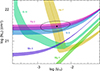 |
Fig. 5. log NH vs. log UH phase-space plot, with constraints based on the measured total ionic column densities (sum of the column densities of the ground state and all the observed excited states). The measurements are shown as solid curves, and the dashed curves show lower limits. The shaded regions denote the errors associated with each Nion. The phase-space solution with minimized χ2 is shown as a black dot surrounded by a black ellipse indicating the 1σ error. |
While we have robust column density measurements from multiple troughs corresponding to Co II and a single trough corresponding to Zn II, we did not use them to constrain our photoionization solution because the ionization structure of the singly-ionized iron-peak elements is very similar to that of Fe II. Their contours in the (NH, UH) phase space shown in Fig. 5 are thereofre parallel to that of Fe II, and the exact location depends on their respective abundances. As Co and Zn are much less abundant than Fe, their ionization structure is more prone to be affected by a slight variation in their abundances as compared to Fe, and we therefore did not include them in our determination of the best-fit photoionization solution.
4. Number density of the outflow
4.1. Electron number density
In the absorption system S2 of the outflow in J0932-0840, we detected multiple troughs arising from excited metastable levels of Fe II (see Fig. 4). Under the assumption of collisional excitation, the ratios of the column densities of these excited lines to the resonance line can be used as an indicator of the electron number density (ne) of the outflow (e.g., de Kool et al. 2001; Arav et al. 2018). To do this, we obtained the theoretical population ratios of the various excited states and the ground state as a function of ne using the CHIANTI atomic database (vers. 9.0 Dere et al. 1997, 2019). We then compared these predictions with our measurements of the column density ratios with the results shown in Fig. 6. The various excited levels constrain log(ne) to be between 3.1 and 3.75 [cm−3]. We determined its weighted mean using the method described by Barlow (2004) and obtained the error using the procedure described in Appendix A. This resulted in log(ne) =  .
.
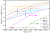 |
Fig. 6. Theoretical population ratios for different Fe II* transitions for Te = 5000 K (determined from our CLOUDY modeling; dashed curves). The solid crosses represent the observed column density ratios and their corresponding error (which includes the error determined in Sect. 3.3). The arrows represent the lower limits obtained from possibly saturated troughs corresponding to these energy levels. The mean ne along with its errors obtained from all the levels is shown in brown. |
In determining ne, we used an effective electron temperature of Te = 5000 K based on the average Fe II temperature determined from our photoionization modeling. This temperature is lower than the common assumption of Te ≈ 10 000 K for photoionized outflows. However, it does not significantly affect our solution for ne as its dependence on the temperature in this range is weak. This can be understood by noting that for a given energy level, the relative excited state population depends on the temperature through the Boltzmann factor e−ΔE/kT, where ΔE is the energy of the transition, and k is the Boltzmann constant. For the FeII* levels used in determining ne, ΔE ≤ 1873 cm−1 and thus, ΔE/k ≲ 2700 K. Therefore, for higher temperatures, the contribution from the Boltzmann factor does not vary significantly, and the dependence of the relative excited state population on the temperature is thus weak.
We also measured the column densities of troughs corresponding to two excited metastable levels of Ni II (and a lower limit for the ground state). However, as Dunn et al. (2010) noted, Ni II cannot be used as a reliable indicator of the electron number density of the outflow because as opposed to Fe II, Ni II is much more prone to fluorescence excitation by the UV continuum (Lucy 1995; Bautista et al. 1996). Therefore, the population of the Ni II excited levels is highly sensitive to the incident radiation, which makes it hard to model its excited-state population. We thus focused solely on Fe II for our density diagnostics.
4.2. Hydrogen number density
We performed a similar analysis for the hydrogen number density (nH) by modeling the photoionized gas using CLOUDY, which offers two advantages over the CHIANTI analysis. First, CLOUDY does not assume fixed values in ne and Te within the gas. For a given value of the gas density nH and a choice of elemental abundances, ne, Te, and the ion number densities are instead computed self-consistently given the depth-dependent thermal and ionization equilibrium solutions determined zone by zone throughout the cloud. Second, since an assumption about the outflow gas density nH is part of the ionization equilibrium solution, there is no need to guess its value based upon the value of ne determined from the level-population or excitation analysis. The CLOUDY models also include the contributions from fluorescence excitation (and other microphysics) in addition to collisional excitation, although this is not expected to significantly affect the relevant Fe II level populations, as mentioned in the previous section.
For our analysis, we ran models for the outflow with fixed NH and UH (obtained from our photoionization modeling in Sect. 3.4) for a range of nH (104.0 ≤ nH (cm−3)≤106.5, in steps of 0.5 dex). These models predict the column densities for all the available levels of Fe II, from which we obtained the column density ratios for the various levels to the ground state and compared them with the ratios obtained from the spectrum. The results of this analysis are shown in Fig. 7.
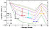 |
Fig. 7. Excited-state to ground-state ratios for Fe II. The dashed lines show the level population ratio predicted by CLOUDY for different values of the hydrogen number density. The measurements are shown as coloured circles and are accompanied by their errors. |
The different excited-state ratios were reproduced for hydrogen number densities between 4.5≲ log(nH) ≲5.0 [cm−3]. To determine the best-fit value of nH from this analysis, we varied log(nH) between 4.0 and 5.5 [cm−3] in steps of 0.1 to create a grid of models. We then compared the observed column density ratios of the excited states with the model predictions to perform a χ2 minimization. This resulted in a best-fit solution with log(nH) = 4.8 [cm−3]. We discuss the relation of the electron number density solution determined using CHIANTI (log(ne) = 3.42 [cm−3]) and the hydrogen number density solution determined from CLOUDY (log(nH) = 4.8 [cm−3]) in the next section.
4.3. Physical structure of the cloud
The formation of Fe II and the excitation of various energy levels are better understood by a detailed examination of the physical structure of the photoionized cloud. As found through the photoionization modeling in Fig. 5, the cloud is bound by a total hydrogen column density of log(NH) = 21.47 [cm−2]. Using log UH = −2.4 and the HE0238 SED, we employed CLOUDY to provide a zone-wise description of the cloud for the best-fit hydrogen number density solution obtained in Sect. 4.2 (log(nH) = 4.8 [cm−3]). Figure 8 shows the obtained physical parameters (Te and ne) and the column densities for the observed Fe II levels as a function of the hydrogen column density within the cloud. We defined the hydrogen ionization front (marked by the dashed black line) as the point in the cloud at which half the hydrogen is ionized, and therefore, the density of fully ionized hydrogen (H II) and neutral hydrogen (H I) is similar.
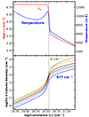 |
Fig. 8. Physical structure of the photoionized cloud vs. the total hydrogen column density for log(nH) = 4.8 [cm−3]. The top panels show the variation in the electron density and temperature within the cloud. The bottoms panels show the cumulative column density of each Fe II level detected in the spectra. The dashed vertical black line marks the H I ionization front. |
Figure 8 (top panel, blue curve) shows that the temperature within the cloud drops suddenly across the H I ionization front because most of the highly energetic photons are absorbed at the front. The electron number density also remains fairly constant before the H I front. In this region, as most of the hydrogen is fully ionized, the electron number density is linearly related to the hydrogen number density with ne≈ 1.2 nH (approximation for fully ionized plasma; Osterbrock & Ferland 2006). However, across the H I front, ne drops suddenly by around an order of magnitude, as shown in Fig. 8 (top panel, red curve). This decrease is attributed to hydrogen becoming neutral and thus absorbing most of the free electrons. The bottom panel shows that the column densities of all observed levels of Fe II also vary rapidly near the front, and a sudden increase occurs just inside. The hydrogen ionization front is essential for the effective formation of Fe II as it acts as a shield against high-energy photons, thus preventing its further ionization. Therefore, most of the observed Fe II comes from the region of the cloud beyond the H I front. The varying electron number densities and temperatures in this region indicate that the conditions that determine the collisional excitation equilibrium are starkly different before and after the H I ionization front. This is an important effect that shows that the majority of Fe II is subjected to a significantly reduced electron number density than the rest of the cloud, where it traces the constant hydrogen number density. Therefore, the approximation ne≈ 1.2 nH is not correct in FeLoBAL outflows, and using this approximation can lead to a severe underestimation for nH.
We estimated the effective Te and ne for Fe II by averaging over all the zones while weighting their contribution based on the their relative Fe II populations. This resulted in Teeff = 5060 K and log(neeff) = 3.51 [cm−3]. This agrees remarkably well with the solution obtained from CHIANTI in Sect. 4.1 with log(ne) =  [cm−3]. This shows that the two solutions obtained independently for ne and nH, respectively, are consistent with each other. We thus adopted log(nH) =
  [cm−3] for the cloud.
We note that this is not the first time a difference between the two density solutions was deduced for a low-ionization quasar outflow. Dunn et al. (2010) found nH for their outflow to be ∼0.4 dex higher than ne. Similarly, de Kool et al. (2001) found that their models required nH to be ∼0.4/1.4 dex higher than ne depending on the choice of the abundance and depletion model. On the other hand, Moe et al. (2009) and Bautista et al. (2010) reported that for their models, ne ≈ nH. These different studies thus revealed that the low-ionization gas in these outflows is subject to a diverse range of physical conditions.
5. Distance and energetics
5.1. Distance to the outflow
After we obtained UH from photoionization modeling (Sect. 3.4) and nH (Sect. 4), we inverted Eq. (4) to obtain the distance of the outflow from the emission source (R) as
 (5)
(5)
To obtain the rate of hydrogen ionizing photons emitted by the source, we scaled the HE0238 SED used in our modeling to match the estimated SDSS flux of J0932+0840 at an observed wavelength of λ≃ 5680 Å, with Fλ = 7.35 × 10⁻¹⁷ erg s−1 cm−2
Å−1. Integrating over the scaled SED for energy values above 1 Ryd. gives us QH =  × 1056 s−1 and bolometric luminosity LBol =
  × 1046 erg s−1. This resulted in a location of the outflow that is
  kpc away from the central source.
5.2. Black hole mass and Eddington luminosity
As described in Sect. 2.2, Mg II 2799 Å is one of the most prominent emission features in the SDSS spectra. Based on the scaling relation derived in Bahk et al. (2019), we estimated the black hole mass (MBH) from the Mg II emission line as
 (6)
(6)
where L3000, 44 is the rest-frame luminosity λLλ at 3000 Å in units of 1044 erg s−1, and the FWHMMg II is in units of 1000 km s−1. Based on our modeling in Fig. 2, FWHMMg II ≈ 3430 km s−1, and from our continuum modeling of the SDSS spectrum at 3000 Å,  × 1046 erg s−1. These values used with Eq. (6) lead to log
 , which results in an Eddington luminosity
  × 1047 erg s−1.
5.3. Energetics
In a simple geometry for the outflow in the form of a partial spherical shell that covers the fractional solid angle Ω and moves with a velocity v, the total mass is (see Borguet et al. 2012 for a detailed discussion)
 (7)
(7)
where R is the distance of the outflow from the source, NH is the total hydrogen column density of the outflow, mp is the proton mass, and μ = 1.4 is the atomic weight of the plasma per proton. Defining the dynamic timescale tdyn = R/v, where v is the outflow velocity, we obtained the mass-flow rate Ṁ and the kinetic luminosity Ėk,
 (8)
(8)
As Ω cannot be determined from the spectrum, the fraction of quasars that show the particular class of outflows has commonly been used as a substitute. Although FeLoBALs are extremely rare, as detailed in the introduction, we used Ω ≈ 0.2, based on the fraction of quasars that show C IV BALs (which is seen in the SDSS spectra of J0932+0840). This is based on the argument by Dunn et al. (2010) based on the morphological indistinguishability of the C IV BALs in FeLoBALs with C IV BALs in the ubiquitous high-ionization BALQSOs. According to this, FeLoBALs fall under the class of normal Ω ≈ 0.2 outflows that are observed through a rare LOS.
This results in a mass-loss rate of Ṁ =  M⊙ yr−1 and kinetic luminosity Ėk =
  × 1043 erg s−1, which is
  × 10−4 of the quasar LEdd and
  × 10−4 of its LBol (see Table 3 for a summary of the obtained parameters for the quasar and its outflow). Hopkins & Elvis (2010) showed that a kinetic luminosity of ∼5 × 10⁻³ of the quasar luminosity is required for an efficient AGN feedback. As the kinetic luminosity of this outflow component is much lower than this requirement, it is not expected to contribute significantly toward AGN feedback processes.
Physical parameters of quasar J0932+0840 and its outflow S2.
6. Discussion
6.1. Variability in the broad absorption lines
As mentioned in Sect. 2, the two different epochs of SDSS spectra were obtained ∼8 years apart, which spans roughly 8/(1 + z)∼2.4 yr in the rest frame of the quasar. We compared them over their common wavelength range (4000–9000 Å in the observed frame) and found no discernible change in the continuum as the flux level remained the same in regions without emission or absorption. The outflow identified in the UVES spectrum is also clearly detected in the SDSS spectra. However, due to its lower resolution, the three narrow low-velocity components (v ∼ −500, −700, and −850 km s−1) appear as a single component, whereas the broader high-velocity components (v ∼ −1300, −4200, and −5000 km s−1) are well resolved. The low-velocity component does not vary significantly over the two epochs for any of the observed ionic species. This is best confirmed by the nonblack troughs corresponding to the low-ionization species (e.g., Si II, Fe II, and Ni II). For the high-ionization species (e.g., C IV, Si IV, and N V), it is harder to determine any variation as their troughs are completely saturated, and thus, it cannot be completely ruled out.
For the broad high-velocity components, however, a clear change is visible as most of the nonblack troughs become considerably shallower. Figure 9 shows this phenomenon for Al III, which shows the most dramatic decrease among all observed species. The low-velocity components for Al III, Si II, and Si II* (marked with vertical black lines) do not show any appreciable variation. However, the high-velocity Al III component (between 6010 < λobs < 6080 Å) shows stronger absorption and a more pronounced kinematic structure for the 2003 spectrum than for the 2012 spectrum. Possible explanations for this variation in the high-velocity structure include (i) transverse motion of the outflowing gas across our line of sight or (ii) a change in the ionization state of the gas. In Sects. 6.1.1 and 6.1.2, we consider these two scenarios.
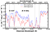 |
Fig. 9. Spectral region around the Al III BAL as observed in the 2003 (in red) and 2012 spectra (in blue). The troughs corresponding to our main outflow system at v ≈−700 km s−1 are marked with a dashed black line. We chose this spectral region as it shows the most noticeable difference in the high-velocity structure between the two epochs. |
6.1.1. Transverse motion
In this case, variability in the troughs is assumed to be due to the transverse motion of the absorbing gas such that its coverage of the continuum source along our line of sight changes. With the help of some simplifying assumptions, we determined the transverse velocity of the variable component and an upper limit for its distance from the central source following previous studies (e.g., Moe et al. 2009; Hall et al. 2011; Yi et al. 2019). Assuming that the black hole accretes close to the Eddington limit, we used its bolometric luminosity and black hole mass to estimate the radius of the accretion disk. Using Eq. (3.15) of Peterson (1997) and the relation of the accretion disk size to black hole mass derived by Morgan et al. (2010), we found the accretion disk radius to be about one light day.
The residual intensity of the Al III component shown in Fig. 9 increases by ∼0.4 in 2.4 yr in the quasar rest frame. In the simplest scenario, this would imply that the transverse motion of the gas allowed it to cross roughly 40% of the two-light-day-wide continuum source in the span of 2.4 yr. This results in a lower limit for the transverse velocity of vtr≳ 275 km s−1. Finally, when we assume that this tangential velocity does not exceed the Keplerian orbital velocity solely due to the SMBH, we obtain an upper limit on the distance of the high-velocity component from the center of R < GMBH/v2 ≈ 70 pc.
However, at these large distances, the outflowing gas could be affected by the potential of the stars in the galactic bulge. We determined whether this contribution is significant by obtaining the radius of influence (rh) of the SMBH. rh is defined as the radius at which the Keplerian rotation velocity equals the velocity dispersion of the galaxy, and it is thus a typical estimate of the radius within which the SMBH must dominate the gravitational potential (Peebles 1972). Using Eqs. (17.1) and (17.6) of Bovy (in prep.)1, we obtained rh ≈ 46 pc. As this is smaller than our upper limit on the distance (70 pc), we needed to include the contribution from the Galactic bulge. Within the sphere of influence, the total mass of the stars is roughly equal to that of the SMBH. We assumed that the density of the galactic bulge is roughly constant around the center (within the scale of a few hundred parsecs) and obtained the enclosed stellar mass as a function of the radius, with M*(< r) ≈ MBH (r/rh)3. Then, we solved for the Keplerian velocity profile as
 (9)
(9)
This revealed that the Keplerian velocity decreases with distance from the center because the mass of stars is initially far lower than that of the SMBH. However, with increasing distance, continually more stellar mass is accumulated and eventually becomes the dominant factor. Therefore, the velocity eventually stops to decrease, with a minimum at r≈ 0.8 rh, beyond which it increases monotonically to the extent of the bulge. In our case, the minimum Keplerian velocity (vmin) ≈ 470 km s−1 is higher than the lower limit on the transverse velocity obtained for the outflowing component. Therefore, we cannot obtain any estimate on the its distance based on the available information about the variability.
Finally, we note that while considering the case for transverse motion of the gas, we assumed that the variable broad structure (with Δv ≳ 3000 km s−1) shown in Fig. 9 is a single outflow component. If this broad feature were composed of different velocity components that could be at different radii from the central source, however, the observed variability would require their coordinated movement, which is unlikely. In this scenario, a change in the ionization state of the gas is a more viable explanation for the variability (see Sect. 5.1 of Capellupo et al. 2013, for a detailed discussion).
6.1.2. Change in ionization state
Because the ionization equilibrium of the outflow is dominated by photoionization, a change in the incident ionizing flux is expected to lead to a change in the ionization state of the absorbing gas, which would then be reflected in the corresponding troughs. In this section, we consider whether this mechanism might explain the nature of the absorption trough variability in the SDSS spectra of J0932+0840. Our model focused on three physical and observational constraints: 1. The plausibility of change in the ionizing flux, 2. a lack of variation in the Si II 1808, 1817 Å troughs for our main outflowing system, and 3. a significant change in the Al IIIλλ 1855, 1863 doublet corresponding to a higher-velocity outflowing system. We discuss each of these in detail below.
1. For J0932+0840, as the spectra do not cover the wavelength region responsible for the ionizing radiation (λrest ≤ 912 Å), we have no direct information about variation in the ionizing flux. In the spectral region covered by the two SDSS epochs (1200 ≲ λrest ≲ 2700 Å), the underlying continuum emission does not change appreciably, which indicates that no drastic changes occur in the shorter wavelength regime because they are usually assumed to be correlated. However, an exception to this correlation has been observed by Arav et al. (2015), and a variation in the ionizing flux therefore cannot be ruled out based on the far-UV flux alone. To study the effect of any possible variation in detail, we considered an example in which the ionizing flux increased by a factor of ∼2 between the two epochs.
2. We first considered the main outflowing component at v ∼ −700 km s−1, for which no significant variation was detected in the nonblack troughs from the low-ionization species (e.g., see the Si II troughs in Fig. 9). To study the maximum variation in the ionization state of the gas as a result of the increase in the ionizing flux, we assumed that a new ionization equilibrium was established over a timescale shorter that the separation between the epochs. Equation (4) shows that the new ionization parameter (UH2012) should then be related to the old ionization parameter (UH2003) as UH2012/UH2003 ∼ 2, while other parameters such as NH and nH remain unchanged. When we assume that the ionization parameter of this component during the 2003 epoch is similar to that obtained from the VLT/UVES spectrum, we have log(UH2003) = −2.4 and log(UH2012) = −2.1. We compared our photoionization models (with log(NH) = 21.5 [cm−2]) of the outflowing gas in both these ionization states and found that the Si II column density decreased by only ∼10% despite the 100% increase in the ionizing flux. To better understand this phenomenon, we tracked the decrease in the Si II column density as a function of NH, and the results are shown in Fig. 10. For the same variation in the ionizing flux, the percentage change in Si II column density can be different by up to an order of magnitude, depending on the total hydrogen column density of the cloud.
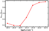 |
Fig. 10. Change in the column density of Si II due to the increase by a factor of 2 in the ionizing flux for clouds with a different total hydrogen column density (NH). For clouds that did not form the H I ionization front (log(NH) ≲ 20.5 [cm−2]), the variation in column density is much higher than for the clouds that formed the ionization front. |
This effect can be understood by noting that the formation of singly-ionized species such as Si II strongly depends on the hydrogen ionization front (see Sect. 4.3), which forms around log(NH) ∼ 20.5 [cm−2] in our case. Before the H I front, only a small fraction of silicon is in the form of Si II, and the majority is in more highly ionized forms (e.g., SiIII/IV). The exact amount of Si II is thus determined by a delicate ionization balance with the higher ionized species, which strongly depends on the incident ionizing flux. Therefore, variations in this flux are reflected strongly in the Si II column density before the H I front. On the other hand, after the front, most of the silicon is found to be in the form of Si II (> 90% for log(NH) ≥ 21.5 [cm−2]). With the increase in the ionizing flux, the H I front shifts to a higher NH, but it still continues to shield the gas behind it from Si II ionizing photons (i.e., photons with an energy greater than the ionization potential of Si II ∼ 16.35 eV) and the ionization balance of silicon there continues to be dominated by Si II. Therefore, the Si II column density for the clouds with higher NH is much less sensitive to the change in the ionizing flux. This is also true for other singly ionized species (e.g., Fe II and Ni II), and thus, their column densities are not expected to vary significantly in the case of our main outflowing component either, which is consistent with our observations.
3. We considered the higher-velocity component at v ∼ −5100 km s−1, which shows troughs from multiple species such as Si II, C II, Al III, Mg II, Si IV, and C IV. The Al IIIλλ 1855, 1863 doublet for this component is shown in Fig. 9 between 6020–6070 Å, where it shows considerable variation between the two epochs. There are also clear signs of variations for the unsaturated troughs of Si II 1260 Å and C II 1335 Å, but the troughs corresponding to Mg II, Si IV, and C IV are saturated, and thus, their variation cannot be characterized properly. While the photoionization solution of this component is not well constrained, we considered whether this variation in the low-ionization components might be understood in terms of a change in the ionization state of the gas. Krolik & Kriss (1996) provided an estimate for the recombination timescale (t*) over which a sudden change in the incident ionizing flux would lead to a change in the ionic fraction of a species. For our main outflowing component, we find  ∼ 1.24 yr. We lack a density diagnostic for the high-velocity component, and we thus cannot obtain its recombination timescale directly. However, we note that due to its much higher velocity, this component is expected to be closer to the central source and thus have a higher hydrogen and electron number density than our main outflowing component (from Eq. (5)). As t* is inversely proportional to ne for similar temperatures, we expect the recombination timescale of the high-velocity component to be significantly shorter than 1.24 yr. It would thus be much shorter that the 2.4 yr span between the two epochs in the quasar rest frame. Therefore, the new Al III column density will agree well with that predicted by the time-independent photoionization equilibrium equations.
To study this variation quantitatively, we first obtained the column density of the Al III 1863 Å trough in the 2003 epoch using Eq. (1). This was done by assuming an AOD model and integrating over the velocity range −5450 ≤ v ≤ −4550 km s−1, which resulted in log(NAl III) = 14.81 [cm−2]. We repeated this process (with the same velocity range) for the 2012 epoch and found log(NAl III) = 14.49 [cm−2]. If this decrease in Al III column density is due to a change in the ionization state, we should be able to find a constant value of NH and the two ionization parameters (UH and U′H) that can reproduce the observed Al III column densities for the two epochs. We again assumed that the ionizing flux increased by a factor of 2 between the two epochs, and therefore, we have UH/U′H = 0.5. With this constraint in mind, we explored a (NH, UH) phase-space plot (similar to Fig. 5) for the measured Al III column densities and obtained log(NH) = 21.1 [cm−2], log(UH) = − 2 and log(U′H) = − 1.7. This variation would also predict a decrease in the column densities of Si II and C II, which is also seen in the observations. On the other hand, the Si IV and C IV column densities would be expected to increase, but this cannot be confirmed as the corresponding troughs are saturated in both epochs. Therefore, our example shows that the observed variability pattern might be due to changes in the ionization state of the gas.
6.2. Previous high-resolution studies of FeLoBAL outflows
In Sect. 4 we highlighted the importance of taking the physical structure of the cloud into account while estimating its nH from the ne determined from observed excited states of low-ionization species such as Fe II. Depending on parameters such as the thickness of the cloud, ne/nH can take values much lower than 1.2. The assumption that the plasma is highly ionized can then lead to an overestimation for the distance of the outflow and its energetics (see Eqs. (5) and (8)).
We found four such cases in the previous high-resolution studies of FeLoBAL outflows with a distance determination in which the effect of the physical structure of the cloud was not considered in their density diagnostics. For each of these objects, we modeled the outflowing cloud using the NH, UH and the incident SED prescribed in the respective analyses. We then ran a grid of models with varying nH to determine the value for which the weighted ne matched the value determined using excited-state ratios observed in their outflow system. Using this new nH, we then reevaluated R, Ṁ, and Ėk for the outflows. Table 4 shows the result of this analysis. For three of these objects, the reevaluated distance determination does not vary significantly from the reported distance. However, for the outflow in J1321-0041, we find that ne/nH ≲ 10−1, and therefore, the distance of the outflow from the central source was overestimated by ∼300%.
Reevaluated density, distance, and energetics for some FeLoBAL outflows from the literature.
7. Summary and conclusion
We identified several outflow systems in the VLT/UVES spectrum of quasar SDSS J0932+0840, and analyzed the system with v ∼ −720 kms−1 in detail.
-
In Sect. 3.1 we outlined our determination of the column densities of several ionic species. This enabled us to employ photoionization modeling (see Fig. 5) for the outflow and obtain its total hydrogen column density
 [cm−2]) and ionization parameter (log UH =
  ).
). -
The detection of several ground- and excited-state transitions of Fe II allowed us to obtain the number density of the outflow. We modeled the electron number density (ne) and hydrogen number density (nH) independently and obtained log(ne) =
 [cm−3] (Sect. 4.1) and log(nH) = 4.80 [cm−3] (Sect. 4.2).
 -
We examined the physical structure of the cloud in Sect. 4.3 and showed that the formation of Fe II is subject to a set of conditions different from most of the cloud, as it takes place beyond the hydrogen ionization front, where ne and temperature drop suddenly (see Fig. 8). For FeLoBAL outflows, the approximation of highly ionized plasma therefore does not hold as ne ≉ 1.2nH.
-
We obtained the effective ne for our modeled cloud with log(nH) = 4.80 [cm−3] as log(neeff) = 3.51 [cm−3]. This agrees with the measured value of log(ne) =
 [cm−3], and we thus showed that our independent solutions for ne and nH are consistent with each other.
 -
Using our obtained solution for nH, we estimated the distance of the outflow to be
 kpc from the central source. This led to
  M⊙ yr−1 and Ėk =
  × 1043 erg s−1, with Ėk/LEdd =
  × 10−4. This outflow is thus not expected to contribute significantly to the AGN feedback.
 -
We compared two epochs of SDSS spectra separated by ∼2.4 years in the quasar rest frame and explained the observed pattern of the absorption variation in terms of a change in the ionization state of the gas.
An online draft of the work is available at https://galaxiesbook.org/
Acknowledgments
We acknowledge support from NSF grant AST 2106249, as well as NASA STScI grants AR-15786, AR-16600, AR-16601 and AR-17556.
References
- Arav, N., De Kool, M., Korista, K. T., et al. 2001a, ApJ, 561, 118 [NASA ADS] [CrossRef] [Google Scholar]
- Arav, N., Brotherton, M. S., Becker, R. H., et al. 2001b, ApJ, 546, 140 [NASA ADS] [CrossRef] [Google Scholar]
- Arav, N., Kaastra, J., Kriss, G. A., et al. 2005, ApJ, 620, 665 [CrossRef] [Google Scholar]
- Arav, N., Moe, M., Costantini, E., et al. 2008, ApJ, 681, 954 [NASA ADS] [CrossRef] [Google Scholar]
- Arav, N., Borguet, B., Chamberlain, C., Edmonds, D., & Danforth, C. 2013, MNRAS, 436, 3286 [NASA ADS] [CrossRef] [Google Scholar]
- Arav, N., Chamberlain, C., Kriss, G., et al. 2015, A&A, 577, A37 [NASA ADS] [CrossRef] [EDP Sciences] [Google Scholar]
- Arav, N., Liu, G., Xu, X., et al. 2018, ApJ, 857, 60 [NASA ADS] [CrossRef] [Google Scholar]
- Badnell, N. 2011, Comp. Phys. Commun., 182, 1528 [NASA ADS] [CrossRef] [Google Scholar]
- Bahk, H., Woo, J.-H., & Park, D. 2019, ApJ, 875, 50 [NASA ADS] [CrossRef] [Google Scholar]
- Barlow, R. 2004, arXiv e-prints [arXiv:physics/0401042] [Google Scholar]
- Bautista, M. A., Peng, J., & Pradhan, A. K. 1996, ApJ, 460, 372 [Google Scholar]
- Bautista, M. A., Dunn, J. P., Arav, N., et al. 2010, ApJ, 713, 25 [NASA ADS] [CrossRef] [Google Scholar]
- Begelman, M. C., & Nath, B. B. 2005, MNRAS, 361, 1387 [NASA ADS] [CrossRef] [Google Scholar]
- Begelman, M. C., & Ruszkowski, M. 2005, Philos. Trans. R. Soc. Lond. Ser. A, 363, 655 [NASA ADS] [Google Scholar]
- Borguet, B. C., Edmonds, D., Arav, N., Dunn, J., & Kriss, G. A. 2012, ApJ, 751, 107 [CrossRef] [Google Scholar]
- Brüggen, M., & Scannapieco, E. 2009, MNRAS, 398, 548 [CrossRef] [Google Scholar]
- Byun, D., Arav, N., & Hall, P. B. 2022a, ApJ, 927, 176 [NASA ADS] [CrossRef] [Google Scholar]
- Byun, D., Arav, N., & Hall, P. B. 2022b, MNRAS, 517, 1048 [NASA ADS] [CrossRef] [Google Scholar]
- Byun, D., Arav, N., & Walker, A. 2022c, MNRAS, 516, 100 [NASA ADS] [CrossRef] [Google Scholar]
- Byun, D., Arav, N., Sharma, M., Dehghanian, M., & Walker, G. 2024, A&A, 684, A158 [NASA ADS] [CrossRef] [EDP Sciences] [Google Scholar]
- Capellupo, D. M., Hamann, F., Shields, J. C., Halpern, J. P., & Barlow, T. A. 2013, MNRAS, 429, 1872 [CrossRef] [Google Scholar]
- Chatzikos, M., Bianchi, S., Camilloni, F., et al. 2023, RMxAA, 59, 327 [NASA ADS] [CrossRef] [Google Scholar]
- Chen, C., Hamann, F., Ma, B., & Murphy, M. 2021, ApJ, 907, 84 [NASA ADS] [CrossRef] [Google Scholar]
- Choi, E., Ostriker, J. P., Naab, T., et al. 2017, ApJ, 844, 31 [NASA ADS] [CrossRef] [Google Scholar]
- Choi, H., Leighly, K. M., Terndrup, D. M., Gallagher, S. C., & Richards, G. T. 2020, ApJ, 891, 53 [NASA ADS] [CrossRef] [Google Scholar]
- Choi, H., Leighly, K. M., Terndrup, D. M., et al. 2022a, ApJ, 937, 74 [NASA ADS] [CrossRef] [Google Scholar]
- Choi, H., Leighly, K. M., Dabbieri, C., et al. 2022b, ApJ, 936, 110 [NASA ADS] [CrossRef] [Google Scholar]
- Ciotti, L., Ostriker, J. P., Gan, Z., et al. 2022, ApJ, 933, 154 [NASA ADS] [CrossRef] [Google Scholar]
- Cochrane, R., Anglés-Alcázar, D., Mercedes-Feliz, J., et al. 2023, MNRAS, 523, 2409 [NASA ADS] [CrossRef] [Google Scholar]
- Dai, X., Shankar, F., & Sivakoff, G. R. 2012, ApJ, 757, 180 [NASA ADS] [CrossRef] [Google Scholar]
- de Kool, M., Arav, N., Becker, R. H., et al. 2001, ApJ, 548, 609 [NASA ADS] [CrossRef] [Google Scholar]
- de Kool, M., Becker, R. H., Arav, N., Gregg, M. D., & White, R. L. 2002a, ApJ, 570, 514 [NASA ADS] [CrossRef] [Google Scholar]
- de Kool, M., Becker, R. H., Gregg, M. D., White, R. L., & Arav, N. 2002b, ApJ, 567, 58 [NASA ADS] [CrossRef] [Google Scholar]
- de Kool, M., Korista, K. T., & Arav, N. 2002c, ApJ, 580, 54 [NASA ADS] [CrossRef] [Google Scholar]
- Dere, K., Landi, E., Mason, H., Fossi, B. M., & Young, P. 1997, A&AS, 125, 149 [NASA ADS] [CrossRef] [EDP Sciences] [Google Scholar]
- Dere, K. P., Del Zanna, G., Young, P. R., Landi, E., & Sutherland, R. S. 2019, ApJS, 241, 22 [Google Scholar]
- Di Matteo, T., Springel, V., & Hernquist, L. 2005, Nature, 433, 604 [NASA ADS] [CrossRef] [Google Scholar]
- Dunn, J. P., Bautista, M., Arav, N., et al. 2010, ApJ, 709, 611 [NASA ADS] [CrossRef] [Google Scholar]
- Edmonds, D., Borguet, B., Arav, N., et al. 2011, ApJ, 739, 7 [NASA ADS] [CrossRef] [Google Scholar]
- Elvis, M. 2000, ApJ, 545, 63 [NASA ADS] [CrossRef] [Google Scholar]
- Fabjan, D., Borgani, S., Tornatore, L., et al. 2010, MNRAS, 401, 1670 [Google Scholar]
- Gallagher, S., Brandt, W., Chartas, G., et al. 2006, ApJ, 644, 709 [NASA ADS] [CrossRef] [Google Scholar]
- Ganguly, R., & Brotherton, M. S. 2008, ApJ, 672, 102 [CrossRef] [Google Scholar]
- Green, P. J., Aldcroft, T. L., Mathur, S., Wilkes, B. J., & Elvis, M. 2001, ApJ, 558, 109 [CrossRef] [Google Scholar]
- Hall, P. B., Anderson, S. F., Strauss, M. A., et al. 2002, ApJS, 141, 267 [NASA ADS] [CrossRef] [Google Scholar]
- Hall, P. B., Anosov, K., White, R., et al. 2011, MNRAS, 411, 2653 [NASA ADS] [CrossRef] [Google Scholar]
- Hamann, F., & Sabra, B. 2004, in AGN Physics with the Sloan Digital Sky Survey, Astronomical Society of the Pacific Conference Series, 311, 203 [NASA ADS] [Google Scholar]
- Hewett, P. C., & Foltz, C. B. 2003, AJ, 125, 1784 [NASA ADS] [CrossRef] [Google Scholar]
- Hidalgo, P. R., Hamann, F., Eracleous, M., et al. 2012, arXiv e-prints [arXiv:1203.3830] [Google Scholar]
- Hopkins, P. F., & Elvis, M. 2010, MNRAS, 401, 7 [NASA ADS] [CrossRef] [Google Scholar]
- Hopkins, P. F., Murray, N., & Thompson, T. A. 2009, MNRAS, 398, 303 [CrossRef] [Google Scholar]
- Hopkins, P. F., Torrey, P., Faucher-Giguère, C.-A., Quataert, E., & Murray, N. 2016, MNRAS, 458, 816 [NASA ADS] [CrossRef] [Google Scholar]
- Knigge, C., Scaringi, S., Goad, M. R., & Cottis, C. E. 2008, MNRAS, 386, 1426 [NASA ADS] [CrossRef] [Google Scholar]
- Korista, K. T., Bautista, M. A., Arav, N., et al. 2008, ApJ, 688, 108 [NASA ADS] [CrossRef] [Google Scholar]
- Krolik, J., & Kriss, G. 1996, ApJ, 456, 909 [NASA ADS] [CrossRef] [Google Scholar]
- Kurucz, R., & Bell, B. 1995, Atomic Line Data (RL Kurucz and B. Bell) Kurucz CD-ROM No. 23. Cambridge, 23 [Google Scholar]
- Leighly, K. M., Terndrup, D. M., Gallagher, S. C., Richards, G. T., & Dietrich, M. 2018, ApJ, 866, 7 [NASA ADS] [CrossRef] [Google Scholar]
- Leighly, K. M., Choi, H., DeFrancesco, C., et al. 2022, ApJ, 935, 92 [NASA ADS] [CrossRef] [Google Scholar]
- Liao, S., Irodotou, D., Johansson, P. H., et al. 2024, MNRAS, 530, 4058 [Google Scholar]
- Lucy, L. 1995, A&A, 294, 555 [NASA ADS] [Google Scholar]
- Lucy, A. B., Leighly, K. M., Terndrup, D. M., Dietrich, M., & Gallagher, S. C. 2014, ApJ, 783, 58 [NASA ADS] [CrossRef] [Google Scholar]
- Moe, M., Arav, N., Bautista, M. A., & Korista, K. T. 2009, ApJ, 706, 525 [NASA ADS] [CrossRef] [Google Scholar]
- Moll, R., Schindler, S., Domainko, W., et al. 2007, A&A, 463, 513 [NASA ADS] [CrossRef] [EDP Sciences] [Google Scholar]
- Morabito, L. K., Dai, X., Leighly, K. M., Sivakoff, G. R., & Shankar, F. 2011, ApJ, 737, 46 [NASA ADS] [CrossRef] [Google Scholar]
- Moravec, E., Hamann, F., Capellupo, D., et al. 2017, MNRAS, 468, 4539 [NASA ADS] [CrossRef] [Google Scholar]
- Morgan, C. W., Kochanek, C., Morgan, N. D., & Falco, E. E. 2010, ApJ, 712, 1129 [NASA ADS] [CrossRef] [Google Scholar]
- Murphy, M. T., Kacprzak, G. G., Savorgnan, G. A., & Carswell, R. F. 2019, MNRAS, 482, 3458 [NASA ADS] [CrossRef] [Google Scholar]
- Murray, N., Chiang, J., Grossman, S., & Voit, G. 1995, ApJ, 451, 498 [NASA ADS] [CrossRef] [Google Scholar]
- Osterbrock, D. E., & Ferland, G. J. 2006, Astrophysics of Gas Nebulae and Active Galactic Nuclei (University Science Books) [Google Scholar]
- Ostriker, J. P., Choi, E., Ciotti, L., Novak, G. S., & Proga, D. 2010, ApJ, 722, 642 [NASA ADS] [CrossRef] [Google Scholar]
- Peebles, P. 1972, ApJ, 178, 371 [NASA ADS] [CrossRef] [Google Scholar]
- Peterson, B. M. 1997, An Introduction to Active Galactic Nuclei (Cambridge University Press) [Google Scholar]
- Planck Collaboration VI. 2020, A&A, 641, A6 [NASA ADS] [CrossRef] [EDP Sciences] [Google Scholar]
- Reichard, T. A., Richards, G. T., Hall, P. B., et al. 2003, AJ, 126, 2594 [NASA ADS] [CrossRef] [Google Scholar]
- Savage, B. D., & Sembach, K. R. 1991, ApJ, 379, 245 [NASA ADS] [CrossRef] [Google Scholar]
- Silk, J., & Rees, M. J. 1998, A&A, 331, L1 [NASA ADS] [Google Scholar]
- Stone, R. B., & Richards, G. T. 2019, MNRAS, 488, 5916 [NASA ADS] [CrossRef] [Google Scholar]
- Trump, J. R., Hall, P. B., Reichard, T. A., et al. 2006, ApJS, 165, 1 [Google Scholar]
- Vestergaard, M. 2003, ApJ, 599, 116 [NASA ADS] [CrossRef] [Google Scholar]
- Voit, G. M., Weymann, R. J., & Korista, K. T. 1993, ApJ, 413, 95 [NASA ADS] [CrossRef] [Google Scholar]
- Walker, A., Arav, N., & Byun, D. 2022, MNRAS, 516, 3778 [NASA ADS] [CrossRef] [Google Scholar]
- Weinberger, R., Su, K.-Y., Ehlert, K., et al. 2023, MNRAS, 523, 1104 [Google Scholar]
- Weymann, R. J., Morris, S. L., Foltz, C. B., & Hewett, P. C. 1991, ApJ, 373, 23 [NASA ADS] [CrossRef] [Google Scholar]
- Xu, X., Arav, N., Miller, T., & Benn, C. 2018, ApJ, 858, 39 [Google Scholar]
- Xu, X., Arav, N., Miller, T., Korista, K. T., & Benn, C. 2021, MNRAS, 506, 2725 [NASA ADS] [CrossRef] [Google Scholar]
- Yi, W., Brandt, W., Hall, P., et al. 2019, ApJS, 242, 28 [NASA ADS] [CrossRef] [Google Scholar]
Appendix A: Error estimation for mean ne
We observed various excited states of Fe II in the system S2 of the outflow. Using the methodology described in Sect. 4.1, we obtained a corresponding electron number density (ne) solution and its errors for each level as shown in Table A.1. To characterize the outflow with a single ne, we obtain the weighted mean using the methodology described by Barlow (2004). To obtain an estimate for the error on the weighted mean, we use two different procedures, which are described below.
ne obtained from CHIANTI for different Fe II level ratios
A.1. Propagating errors associated with each measurement
One way to estimate error for the mean is to obtain the mean of the weighted errors added in quadrature. If the positive/negative error for the ith measurement of x (xi) is denoted as (δxi)±, then the positive/negative error for the mean, (δ⟨x⟩)±, can be obtained as:
 (A.1)
(A.1)
where wi is the weight associated with each measurement as described in Barlow (2004). With x = log(ne), we obtain (δ⟨log(ne)⟩)+ = 0.24 and (δ⟨log(ne)⟩)− = 0.14, and therefore we have ⟨log(ne)⟩ =  . While this is a robust method to take into account the errors associated with each measurement, it does not include information about the scatter in the values between measurements obtained from the different levels.
A.2. Standard deviation including the measurement errors
To obtain errors on the mean in a way which includes the spread of the measurements around it, and also their own individual errors, we define:
 (A.2)
(A.2)
where N is the total number of measurements and ⟨x⟩ is their mean. With x = log(ne), this definition leads to (δ⟨log(ne)⟩)+ = 0.65 and (δ⟨log(ne)⟩)− = 0.46, and therefore we have ⟨log(ne)⟩ =  . We adopt this value for our analysis and represent it graphically in Fig. 6. It shows that given the scatter between the different measurements, Eq. (A.2) provides a much better representation of the error compared to the smaller values obtained from Eq. (A.1).
All Tables
Absorption lines identified in the VLT spectrum of SDSS J0932+0840 and their measured column densities.
Comparison between the gf values obtained from our calculations and the values available in the NIST database for a sample of transitions.
Reevaluated density, distance, and energetics for some FeLoBAL outflows from the literature.
All Figures
|
Fig. 1. Non-normalized SDSS spectra of J0932+0840 (2012 epoch). The flux density (Fλ) is shown in black, and the error is plotted in gray. |
| In the text | |
|
Fig. 2. Gaussian model fit for the Mg II 2799 emission feature (shown in red). Due to high absorption, the data points for the fit were selected manually. The dashed red line marks the centroid of the best-fit model we used to determine the redshift of the quasar. The dashed blue line shows the continuum level. The error on the flux is shown in gray. |
| In the text | |
|
Fig. 3. Normalized UVES spectrum of J0932-0840. Important features and multiplets are marked in blue, and the identified absorption troughs from the primary outflow system at v ≈ −720 km s−1 are marked with dashed red lines. The zero flux level is shown by the dashed blue lines. The dashed black lines mark troughs from an intervening system at z = 1.28. |
| In the text | |
|
Fig. 4. Identified Fe II troughs for outflow system S2. The histograms show the VLT/UVES spectra in velocity space, and the corresponding dashed curves show the modeled Gaussian for the absorption. The model is based on the 1278 Å transition, and its template with fixed centroid and width was scaled to match the depth of all other troughs. The lower-energy level of the transition and the wavelengths are given for each panel. |
| In the text | |
|
Fig. 5. log NH vs. log UH phase-space plot, with constraints based on the measured total ionic column densities (sum of the column densities of the ground state and all the observed excited states). The measurements are shown as solid curves, and the dashed curves show lower limits. The shaded regions denote the errors associated with each Nion. The phase-space solution with minimized χ2 is shown as a black dot surrounded by a black ellipse indicating the 1σ error. |
| In the text | |
|
Fig. 6. Theoretical population ratios for different Fe II* transitions for Te = 5000 K (determined from our CLOUDY modeling; dashed curves). The solid crosses represent the observed column density ratios and their corresponding error (which includes the error determined in Sect. 3.3). The arrows represent the lower limits obtained from possibly saturated troughs corresponding to these energy levels. The mean ne along with its errors obtained from all the levels is shown in brown. |
| In the text | |
|
Fig. 7. Excited-state to ground-state ratios for Fe II. The dashed lines show the level population ratio predicted by CLOUDY for different values of the hydrogen number density. The measurements are shown as coloured circles and are accompanied by their errors. |
| In the text | |
|
Fig. 8. Physical structure of the photoionized cloud vs. the total hydrogen column density for log(nH) = 4.8 [cm−3]. The top panels show the variation in the electron density and temperature within the cloud. The bottoms panels show the cumulative column density of each Fe II level detected in the spectra. The dashed vertical black line marks the H I ionization front. |
| In the text | |
|
Fig. 9. Spectral region around the Al III BAL as observed in the 2003 (in red) and 2012 spectra (in blue). The troughs corresponding to our main outflow system at v ≈−700 km s−1 are marked with a dashed black line. We chose this spectral region as it shows the most noticeable difference in the high-velocity structure between the two epochs. |
| In the text | |
|
Fig. 10. Change in the column density of Si II due to the increase by a factor of 2 in the ionizing flux for clouds with a different total hydrogen column density (NH). For clouds that did not form the H I ionization front (log(NH) ≲ 20.5 [cm−2]), the variation in column density is much higher than for the clouds that formed the ionization front. |
| In the text | |
Current usage metrics show cumulative count of Article Views (full-text article views including HTML views, PDF and ePub downloads, according to the available data) and Abstracts Views on Vision4Press platform.
Data correspond to usage on the plateform after 2015. The current usage metrics is available 48-96 hours after online publication and is updated daily on week days.
Initial download of the metrics may take a while.