© The Authors 2025

1. Introduction

Quasar outflows are essential components of the feedback mechanisms that regulate the evolution of galaxies and the intergalactic medium (e.g., Silk & Rees 1998; Scannapieco & Oh 2004). These powerful winds can impact the star formation within their host galaxies and contribute to the metal enrichment in the surrounding environment. Outflows are frequently observed in quasar spectra as blueshifted absorption troughs. These absorption outflows are invoked as potential contributors to active galactic nuclei (AGN) feedback processes (e.g., Silk & Rees 1998; Scannapieco & Oh 2004; Yuan et al. 2018; Vayner et al. 2021; He et al. 2022).

Absorption lines in rest-frame UV spectra are generally classified into three categories based on their width: broad absorption lines (BALs) with widths of ≥2000 km s⁻¹, narrow absorption lines (NALs) with widths of ≤500 kms⁻¹, and an intermediate group referred to as mini-BALs (Itoh et al. 2020). While BAL outflows were studied extensively (Vestergaard 2003; Gabel et al. 2006), less is known about NAL outflows.

The chemical abundances of an outflow can be determined by comparing the ionic column densities measured from the absorption lines across the spectrum with the results of photoionization analyses (Gabel et al. 2006; Arav et al. 2007). The primary advantage of using absorption lines over emission lines in abundance studies is that they are able to provide diagnostics that are less dependent on the temperature and density (Hamann 1998; Borguet et al. 2012b). Since BALs present challenges for determining abundances due to their complex nature, with lines often being blended and heavily saturated, we used NALs to determine the abundances. This study focuses on a NAL outflow in the quasar 3C298, and we used archival HST/FOS¹ data to determine the absolute abundances of nitrogen and sulfur, along with physical conditions such as the electron number density.

While not many studies have focused on the abundance of quasar outflows, supersolar abuncances were reported in most of the available literature. For instance, Fields et al. (2005) and Arav et al. (2007) indicated that the outflow in the quasars they studied was significantly enriched, and the abundances often exceeded solar values (Grevesse et al. 2010) by factors of several. Gabel et al. (2006) reported that the absorption outflow in QSO J2233-606 had supersolar abundances of carbon, nitrogen, and oxygen by roughly a factor of 10 (see Table 1). The nitrogen abundance was most enhanced. As investigated by Arav et al. (2020), the absorption outflow in NGC 7469 also exhibits a supersolar abundance, and the carbon and nitrogen abundances are roughly twice and four times the solar values, respectively. However, our analysis of the outflow seen in quasar 3C298 indicates that the abundances of nitrogen and sulfur are 0.4–3 times their solar values, but they can extend to sub- and supersolar values when different spectral energy distributions are considered (see Sect. 3.2). These findings are consistent with recent studies that suggested that radio-loud quasars tend to exhibit a slightly subsolar metallicity in their line-emitting regions, while radio-quiet quasars may show abundances closer to solar values. For example, Punsly et al. (2018) examined the metallicity of the broad-line region (BLR) in NGC 1275, which is a nearby radio-loud AGN with a powerful jet. The findings indicated that its metallicity levels are near solar, which is consistent with Seyfert galaxies and supports a scenario of moderate enrichment that is likely driven by jet and accretion activity. Marziani et al. (2023) revealed that radio-quiet quasars generally have slightly subsolar or solar metallicities, without a significant supersolar enrichment. In contrast, radio-loud quasars tend to exhibit distinctly subsolar metallicities that are often lower than their radio-quiet counterparts. In a more recent study, Floris et al. (2024) focused on the BLR of AGNs in different populations in the quasar main sequence. The study revealed a systematic metallicity gradient along the quasar main sequence, from subsolar levels in Population B quasars (specifically, radio-loud ones) to extremely high supersolar values in extreme Population A (xA) sources. Villar-Martin et al. (2024) observed a subsolar metallicity in the giant nebula associated with the Teacup quasar. However, within the AGN-driven bubble, their study identified a solar or slightly supersolar metallicity. This highlights the complexity of the metallicity distribution in AGN environments, in which a localized metal enrichment occurs within the outflow structures. The use of multiple SEDs (MF87, UV-soft, and HE0238) allows us to assess the impact of varying radiation fields on the derived chemical abundances and to constrain the conditions of the outflow in 3C298.

The detailed analysis of Punsly et al. (2022) of the radio lobes of 3C298 estimated one of the largest known long-term jet powers at 1.28 × 10⁴⁷ erg s⁻¹ and identified a weakly ionizing continuum. In contrast, our study focuses on the chemical abundances of nitrogen and sulfur in the NAL outflow. This offers insights into the physical conditions of the NAL outflow and its role in quasar feedback.

In the following sections, we discuss the observational data, the method we used to derive the abundances from absorption lines, and additional relevant analyses. The results presented here emphasize the importance of considering a broader range of abundances in quasar outflows, and they underscore the necessity for further research in this relatively underexplored field.

This paper is structured as follows. In Sect. 2 we present the observational data, including the spectral data from quasar 3C298 and the relevant absorption lines. Section 3 details the method we employed to derive elemental abundances from these absorption lines, with a focus on the techniques we used to extract the ionic column densities and photoionization modeling, and the determination of the electron number density. Finally, Section 4 concludes the paper with a summary of the key findings. Additionally, Appendices A and B provide detailed error calculations related to the methods we used.

We adopted a standard ΛCDM cosmology with h = 0.677, Ω_m = 0.310, and Ω_Λ = 0.690 (Planck Collaboration VI 2020). We used the Python astronomy package Astropy (Astropy Collaboration 2013, 2018) for our cosmological calculations, as well as Scipy (Virtanen et al. 2020), Numpy (Harris et al. 2020), and Pandas (Reback et al. 2021) for most of our numerical computations. For our plotting purposes, we used Matplotlib (Hunter 2007).

2. Observations

The bright radio source QSO 3C298 lies at redshift z = 1.4362 (based on the NASA/IPAC Extragalactic Database² and also de Diego et al. (2007)), with J2000 coordinates at RA = 14:19:08.18, Dec = +06:28:34.80. Table 1 of Punsly et al. (2022) summarizes the radio data available for this object. The quasar was observed using the HST/FOS on two separate occasions on August 15, 1996, as part of HST Hamann (1996) (PI: Hamann). These observations had exposure times of 1.6 and 2.4 ks, and both used the G270H grating with a central wavelength of 2650 Å. We coadded these two spectra and binned them by three pixels to prepare the data for the further analysis.

After obtaining the relevant data from the Mikulski Archive for Space Telescopes (MAST), we detected an outflow at a velocity of v_centroid = −210 km s⁻¹, with blueshifted ionic absorption lines that are denoted by vertical red lines in Fig. 1.

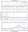Fig. 1. Spectrum of 3C298 observed by HST/FOS in August 1996. The absorption features of the outflow with a velocity of −210 km/s are marked with red lines, and the gray lines show the absorption from the interstellar medium.

3. Analysis

The identified absorption lines in the spectra are shown in Fig. 1. We excluded the C IIIλ977.02Å and O VI doublet absorption lines (λλ 1031.91,1037.61Å) from our analysis since they are observed to be very deep (especially compared to the Lyα absorption line), which suggests that these absorption lines are most likely saturated. We also focused on using Lyϵ of the available Lyman lines because it is the least saturated line of the series.

3.1. Determining the ionic column density

The determination of the ionic column densities (N_ion) of the absorption lines is the first step to understand the physical characteristics of the outflow. The apparent optical depth (AOD) is one method for measuring the ionic column densities using the absorption lines. This approach assumes that the outflow uniformly and completely covers the source (Spitzer 1968; Savage & Sembach 1991). When the AOD method is used, the column density can be determined using Eqs. (1) and (2) below (Spitzer 1968; Savage & Sembach 1991; Arav et al. 2001),

$$\begin{array}{c}\hfill I(v)=e^{-\tau (v)},\end{array}$$(1)

$$\begin{array}{c}\hfill N_{\text{ion}}=\frac{3.77\times {10}^{14}}{{\lambda }_{0}f}\times {\displaystyle \int \tau }(v)dv[{\text{cm}}^{-2}],\end{array}$$(2)

where

I(v) Normalized intensity profile as a function of velocity.

τ(v) Optical depth of the absorption trough.

λ₀ Transition wavelength.

f Oscillator strength of the transition.

To determine the ionic column densities of the Lyϵ, N IIIλ989.80Å, and NIII*λ991.58Å, we opted for the AOD technique because these ions are all singlets. The absorption troughs of these ions are much more shallow than those of other absorption lines (particularly compared to the Lyα), which ensures that they are not saturated and their column density measurements via the AOD method are reliable. For the case of S VI, we only considered its red trough (S VIλ944.52Å) and treated it as a singlet because the red trough exhibits lower noise levels than the blue trough. This makes its measurements more reliable. For more details regarding the AOD method, we refer to Arav et al. (2001), Gabel et al. (2003), and Byun et al. (2022c).

The second method is the partial covering (PC) method, which we applied when two or more lines originated from the same lower level. This approach assumes a homogeneous source that is partially covered by the absorption outflow (Barlow et al. 1997; Arav et al. 1999a,b). By using the PC method and deducing a velocity-dependent covering factor, we ensured that phenomena such as nonblack saturation were considered (de Kool et al. 2002). In this method, the covering fraction C(v) and the optical depth τ(v) are calculated using Eqs. (3) and (4) (Arav et al. 2005). For a doublet transition in which the blue component has twice the oscillator strength of the red component,

$$\begin{array}{c}\hfill I_R(v)-[1-C(v)]=C(v)e^{-\tau (v)}\end{array}$$(3)

and

$$\begin{array}{c}\hfill I_B(v)-[1-C(v)]=C(v)e^{-2\tau (v)},\end{array}$$(4)

in which I_R(v) and I_B(v) are the normalized intensity of the red and blue absorption feature (as shown in Fig. 2), respectively, while τ(v) is the optical depth profile of the red component.

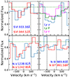Fig. 2. Normalized flux vs. velocity for the blueshifted absorption lines detected in the spectrum of 3C298. The dashed horizontal green line shows the continuum level, and the vertical dashed black lines show the integration region for each line.

We applied the PC method to the N V doublet (λλ1238.82, 1242.80Å). The S/N of the data is moderate, and some of the red doublet flux values are therefore lower than the blue flux values at the same velocity (see Fig. 2). This situation does not allow a PC solution. We therefore modeled each trough with a Gaussian in flux space, in which both Gaussians had the same centroid velocity (v_centroid) and width (see Fig. 3). We then performed the PC method on the resultant Gaussians and converted the resultant τ(v) and C(v) into the column density. For a detailed explanation of the two methods, to better understand the logic behind them, and for a sense of their mathematics, we refer to Barlow et al. (1997), Arav et al. (1999a,b), de Kool et al. (2002), Arav et al. (2005), Borguet et al. (2012a), Byun et al. (2022b,c).

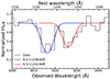Fig. 3. Gaussian modeling of the N Vλ1238.82Å and N Vλ1242.80Å absorption trough.

For each of the absorption lines, we used the redshift of the outflow (z_outflow = 1.4345) to transfer the spectrum from wavelength space to velocity space (see Fig. 2). When performing column density calculations, we chose a velocity range of −750 to +500 km s⁻¹ as our integration range for S VI, Lyϵ, and N V. For N III, and NIII* ions, the integration range is smaller because the absorption trough is narrower (see Fig. 2). The integration ranges for each ion are indicated by vertical dashed lines. We also included Lyγ and Lyδ in Fig. 2 for comparison purposes.

Before we finalized our results, it was essential to estimate the uncertainties arising from systematic errors. To achieve this, we repeated the column density calculations while adjusting for the upper and lower thresholds of the local continuum (as shown in Fig. 4). The finally adopted errors for the column densities of Lyϵ, N III, NIII*, and S VI were determined by quadratically combining the AOD errors with the systematic errors arising from the 5% uncertainty in the local continuum level. For N V, the errors were directly derived from the Gaussian fits. Table 2 summarizes the results of our N_ion measurements, along with their associated uncertainties.

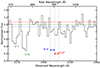Fig. 4. Absorption line profiles for the quasar 3C298, plotted against velocity in km s−1 in the regions around N III and NIII*. The normalized flux is shown on the y-axis, and the absorption lines of Lyϵ, C III, N III, and NIII* are labeled. The dashed green line shows the local continuum model, and the dashed red and dotted blue lines show the ±5% uncertainties. The integration range for N III and NIII* is also shown with blue and red arrows, respectively.

3.2. Photoionization solution

At this stage, we used the ionic column densities to determine the total hydrogen column density (N_H) and the ionization parameter (U_H) following established methods (e.g., Xu et al. 2019; Byun et al. 2022a,b,c; Walker et al. 2022; Dehghanian et al. 2024). We employed the code Cloudy (Gunasekera et al. 2023) to generate a grid of (N_H) and (U_H) values, which allowed us to compare theoretical predictions with observational data that are available in Table 2. The photoionization state of an outflow is influenced by the spectral energy distribution (SED) incident upon it. To evaluate how the choice of SED affects our abundance determination results, we conducted our analysis using three different SEDs: HE0238, MF87, and UV-soft, as shown in Fig. 5. This figure also displays the SED generated for 3C298 by Punsly et al. (2022) (shown in green). The ionizing portion of the SED is critical for our study. As illustrated in Fig. 5, the 3C298 SED from the value reported in Punsly et al. (2022) at log(ν)≈15.7 [Hz] is only 0.1 dex lower than the HE0238 νL_ν at the same frequency, indicating general agreement in the ionizing range. However, we excluded the 3C298 SED from our analysis because the data points in this crucial region were limited.

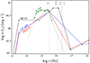Fig. 5. Three SEDs used in the analysis (from Arav et al. 2013) along with the 3C298 SED generated by Punsly et al. (2022). The vertical dashed lines show the ionization energy for each labeled ion.

3.2.1. HE0238 SED

First, we adopted the SED of quasar HE0238-1904 (hereafter HE0238, Arav et al. 2013) and performed Cloudy simulations. HE0238 is the most empirically determined SED in the extreme-ultraviolet (EUV) region and provides a reliable model for studying ionization processes in AGN outflows.

Figure 6 illustrates the results for H I (estimated based on Lyϵ), N III, N V, and S VI, assuming solar abundances. As this figure shows, while there is a photoionization solution (shown by the black dot) that reproduces the N III, N V, and S VI ionic column densities, it does not simultaneously reproduce the observed column density of H I. This discrepancy suggests that the assumption of solar abundances fails to account for all of the observed ionic column densities.

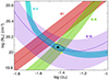Fig. 6. Photoionization solution for the outflow detected in 3C 298. Each colored contour indicates the ionic column densities consistent with the observations (presented in Table 2), assuming the HE0238 SED and solar abundances. The solid lines show the measured value, and the shaded bands show the uncertainties. The black dot shows the best solution for N III and N V, and the 1σ uncertainty is shown by the black oval. The two yellow crosses show the allowed uncertainty region we used to determine the absolute abundances (see Appendix A).

The H I column density predicted by the photoionization model presented in Fig. 6 is $1.{66}_{-0.50}^{+0.61}$ times lower than the observed value (see Appendix A for detailed calculations). This finding indicates that adjustments to the photoionization models are necessary for a more accurate model of the absorption outflow. The only free parameters in the photoionization modeling (in addition to the choice of SED) are the absolute abundances of nitrogen and sulfur. By decreasing the absolute abundances of nitrogen by a factor of 1.66, we can achieve a minimized-χ² solution that reproduces the observations,

$$\begin{array}{cc}\hfill \frac{\text{Expected Abundances of N}}{\text{Solar Abundances of N}}& =\frac{1}{1.{66}_{-0.50}^{+0.61}}=0.{60}_{-0.16}^{+0.26}\hfill \\ \hfill & \to [\text{N}/\text{H}]=-0.{22}_{-0.14}^{+0.16}.\hfill \end{array}$$

Similarly, since the contour of S VI nearly coincides with the crossing point of the N III and N V lines, we can estimate that its abundances have to be adjusted by the same value,

$$\begin{array}{c}\hfill [\text{S}/\text{H}]=-0.{22}_{-0.14}^{+0.16}.\end{array}$$

It is worth mentioning that the notation [X/H] is commonly used to express the abundance of element X relative to hydrogen (H), compared to the same abundance ratio in the Sun. This value is usually reported on a logarithmic scale.

To confirm that the nitrogen and sulfur abundances must be subsolar, we conducted a new set of Cloudy simulations, assuming solar abundances for all elements except for nitrogen and sulfur, for which we scaled its abundance to 60% of their solar values (as calculated above). The results are presented in Fig. 7, which displays the final photoionization solution for the outflow, assuming the HE0238 SED and adjusted abundances for nitrogen and sulfur. As shown in this figure, for the HE0238 SED, the assumption of a subsolar nitrogen and sulfur abundance yields a photoionization solution with ${\chi }_{\mathrm{reduced}}^2=0.01$, indicating an excellent fit for the outflow. Below, we repeat these analyses for two more SEDs. As this figure illustrates and in contrast with our previous modeling, the minimized-χ² photoionization solution that reproduces the observed value of N III and N V (black dot in Fig. 8) overproduces hydrogen. This solution does not produce the observed column density of S VI either. However, its predictions of S VI are still within the measured uncertainties.

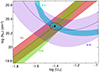Fig. 7. Photoionization solution for the outflow in 3C298, assuming the HE0238 SED and solar abundance for all elements, except for nitrogen and sulfur. The abundances of nitrogen and sulfur are set to be 60% of their solar value with respect to hydrogen.

Fig. 8. Same is Fig. 6, using the MF87 SED and solar abundances.

3.2.2. M87 SED

The second SED we employed is the MF87 SED, which was designed by Mathews & Ferland (1987) to model the energy distribution from the UV-FUV bump to the X-ray regime, and which has been widely used to model radio-loud quasars. Figure 8 shows the results of the photoionization modeling using this SED and assuming solar abundances.

The H I column density predicted by the photoionization solution presented by the black dot in Fig. 8 is approximately $0.6_{-0.18}^{+0.22}$ times the observed value (the error calculation follows the procedure explained in Appendix A). This means that for a solution that produces the observed values of nitrogen and hydrogen at the same time, we have to increase the nitrogen abundance (with respect to those of hydrogen),

$$\begin{array}{cc}& \frac{\text{Expected Abundances of N}}{\text{Solar Abundances of N}}(\text{with respect to H})=\frac{1}{0.6_{-0.18}^{+0.22}}\hfill \\ \hfill & =1.{66}_{-0.44}^{+0.72}\to [\text{N}/\text{H}]=0.{22}_{-0.13}^{+0.16}.\hfill \end{array}$$

We must also adjust the sulfur abundances to reproduce the observations simultaneously. In Fig. 8, we match the S VI contour with the crossing point of N III and N V,

$$\begin{array}{c}\hfill \frac{\text{Expected Abundance of S}}{\text{Solar Abundance of S}}(\text{with respect to N})=1.3_{-0.5}^{+0.5},\end{array}$$

which results in

$$\begin{array}{cc}& \frac{\text{Expected Abundance of S}}{\text{Solar Abundance of S}}(\text{with respect to H})=\hfill \\ \hfill & 1.3_{-0.5}^{+0.5}\times 1.{66}_{-0.44}^{+0.72}=2.{16}_{-1.0}^{+1.2}\to [\text{S}/\text{H}]=0.{33}_{-0.27}^{+0.20},\hfill \end{array}$$

in which the error calculations are similar to those explained in Appendix A.

3.2.3. UV-soft SED

Finally, we investigated the change in the photoionization solution when we employed the UV-soft SED to the outflow. This SED is typically used for high-luminosity radio-quiet quasars and was described in Dunn et al. (2010), Arav et al. (2013). Unlike the MF87 SED, which features a prominent UV bump, the UV-soft model excludes this feature and offers a cooler accretion disk with a power-law spectrum from the near-infrared to X-rays.

Figure 9 shows the results of photoionization simulations of the outflow in 3C298 while considering the UV-soft SED and solar abundances. As this figure shows, a single photoionization solution can reproduce all observed column densities simultaneously:

Fig. 9. Same is Fig. 6, using the UV-soft SED and solar abundances.

$$\begin{array}{cc}& \frac{\text{Expected Abundances of N}}{\text{Solar Abundances of N}}(\text{with respect to H})=\hfill \\ \hfill & \frac{1}{0.{87}_{-0.22}^{+0.32}}=1.{15}_{-0.30}^{+0.40}\to [\text{N}/\text{H}]=0.{06}_{-0.13}^{+0.13},\hfill \end{array}$$

and

$$\begin{array}{c}\hfill \frac{\text{Expected Abundances of S}}{\text{Solar Abundances of S}}(\text{with respect to N})=0.{93}_{-0.4}^{+0.4},\end{array}$$

which results in

$$\begin{array}{cc}& \frac{\text{Expected Abundances of S}}{\text{Solar Abundances of S}}(\text{with respect to H})=\hfill \\ \hfill & 1.{15}_{-0.30}^{+0.40}\times 0.{93}_{-0.4}^{+0.4}=1.{07}_{-0.54}^{+0.60}\to [\text{S}/\text{H}]=0.{03}_{-0.28}^{+0.20}.\hfill \end{array}$$

To summarize the results derived from all three SEDs, we found that the nitrogen and sulfur abundances are consistent with solar values, with a small spread introduced by the choice of the SED. Table 1 presents the final photoionization solution for each SED after adjusting the nitrogen and sulfur abundances according to the calculations above. Based on this table, and by considering the variations introduced by the three SEDs, we report that the total hydrogen column density of the outflow in 3C298 is log(N_H) = 20.05 ± 0.3 [cm⁻²]. This value represents the median of the three measurements, and the uncertainties are chosen to encompass the full range of results from the different SEDs. Similarly, for the ionization parameter, we report log$(U_{\mathrm{H}})=-1.6_{-0.15}^{+0.25}$, where the uncertainties similarly account for the full variation in the SED models.

3.3. Electron number density

We used the Chianti 9.0.1 atomic database (Dere et al. 1997, 2019) to calculate the abundance ratios of the excited state to the resonance state for N III as a function of electron number density (n_e). The Chianti atomic database uses the atomic data for N III, including energy levels, radiative transition rates, and collisional excitation rates. For a given temperature, Chianti then calculates the column density ratio of NIII* to N III as a function of n_e (see the blue curve in Fig. 10). These calculations were performed considering a temperature of 16,000 K, which is predicted by Cloudy for the outflow in 3C298, and by adopting the UV-soft SED. Figure 10 presents the results. Based on Table 2, the column density of the excited state to that of the ground state is $\frac{N_{\mathrm{N}\mathrm{I}\mathrm{I}\mathrm{I}\ast }}{N_{\mathrm{N}\mathrm{I}\mathrm{I}\mathrm{I}}}\approx 1.8$ (marked by the red dot in Fig. 10), which corresponds to log(n_e) = 4.2 [cm⁻³].

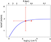Fig. 10. Excited state (E = 174.4 cm−1) to resonance state column density ratio of N III vs. the electron number density (blue curve) from the Chianti atomic database for T = 16 000 K. The measured ratio is shown by the red dot, and the accompanying error bars are shown by the vertical red lines. The 174.4 cm−1 transition in N III arises from the 2P3/2  →  2P1/2 transition within this ion.

To determine the uncertainties on the electron number density, we first determined the uncertainties on the column density ratio to be $\frac{N_{\mathrm{N}\mathrm{I}\mathrm{I}\mathrm{I}\ast }}{N_{\mathrm{N}\mathrm{I}\mathrm{I}\mathrm{I}}}=1.8_{-0.7}^{+1.9}$, as outlined in detail in Appendix B. These uncertainties, represented by vertical red lines in Fig. 10, were then used to calculate the corresponding errors in the electron number density: The upper uncertainty on the column density allows an n_e of infinity, and the result therefore is a lower limit on n_e. The lower uncertainty allows a value of log(n_e) = 3.3 [cm⁻³], as this is the point where the error intersects the theoretical curve. Combining these results and based on the Chianti plot shown in Fig. 10, we conclude that log(n_e)≥3.3 [cm⁻³].

The top horizontal axis of Fig. 10 shows the distance between the outflow and the central source in parsecs, derived from the definition of the ionization parameter (Osterbrock & Ferland 2006),

$$\begin{array}{c}\hfill U_{}\text{H}\equiv \frac{Q_{\text{H}}}{4\pi R^{2}c{n}_{\text{H}}}\Rightarrow R=\sqrt{\frac{Q_{\text{H}}}{4\pi c{n}_{\text{H}}{U}_{\text{H}}}},\end{array}$$(5)

in which Q_H is the number of hydrogen-ionizing photons emitted by the central object per second, R is the distance between the outflow and the central source, n_H is the hydrogen number density, and c is the speed of light. For a highly ionized plasma, we can assume n_e ≈ 1.2 n_H (Osterbrock & Ferland 2006). For 3C 298, Q_H = 1.2 × 10⁵⁷ s⁻¹, which was calculated using the quasar redshift and our adopted cosmology (see Sect. 1). To calculate Q_H, we also scaled the UV-soft SED to match the continuum flux of 3C298 at an observed wavelength of λ = 2650 Å.

Using the ionization parameter resulting from the photoionization modeling with solar abundances (log(U_H) =  − 1.6) and the electron number density from Chianti database (log(n_e) = 4.2 [cm⁻³]), we located the outflow at a distance of approximately 1050 pc from the central source. By considering the lower uncertainties on the electron number density, the outflow might be located as far away as R_max = 2800 pc.

4. Summary

We used archival data from the Hubble Space Telescope and employed a photoionization modeling to determine the absolute abundances of nitrogen and sulfur in the absorption outflow seen in quasar 3C298. Our main conclusions are summarized below.

1. We employed three different SEDs to determine the chemical abundances in the outflow. The use of UV-soft and MF87 SEDs resulted in solar and supersolar abundances, respectively, which agrees with the chemical abundances determined in other quasar outflows, as presented in Table 3. However, when we used the HE0238 SED as the incident SED, our simulations indicated that the nitrogen and sulfur abundances are 60% of their solar values compared to hydrogen. To conclude, each SED we explored produced a distinct regime of potential nitrogen and sulfur abundances. The three SEDs span an abundance range of 0.4–3 times solar.

   Table 3.

   Chemical abundances in outflows.

2. The photoionization modeling assuming three SEDs resulted in three pairs of solutions for log(N_H) and log(U_H) (see Table 1), or an average of log$(N_{\mathrm{H}})=20.{05}_{-0.3}^{+0.3}$ and log$(U_{\mathrm{H}})=-1.6_{-0.15}^{+0.25}$ for the outflow, in which we considered the systematic errors arising from various SEDs.

3. We used the Chianti atomic database to derive the electron number density in the outflow. By comparing the ratio of the excited state to the resonance state of N III, we determined that log(n_e) = 4.2 [cm⁻³], which places the outflow at 1050 pc away from the AGN. However, by taking the uncertainties of the electron number density into account, we estimated that the electron number density is log(n_e)≥3.3 [cm⁻³]. This means that the outflow could be as far away as 2800 pc. One possible scenario to explain the subsolar abundances results is that this outflow is located at this farther distance and is therefore less enriched than outflows closer to the center of the galaxy.

4. Our findings suggest that the outflow system has solar metallicity, with an uncertainty of 60%. The 60% uncertainty in our metallicity determination arises from three different SEDs we considered, that is, MF87, UV-soft, and HE0238. These SEDs represent different assumptions about the ionizing radiation field, which in turn influence the ionization parameter and column density calculations.

5. While subsolar metallicities have been suggested in previous studies (e.g., Arav et al. 2007; Punsly et al. 2018; Marziani et al. 2023; Floris et al. 2024), our analysis contributes to refining the metallicity range by testing multiple SEDs. Our study serves as a complementary analysis that extends the findings of previous AGN feedback studies by exploring the effects of different SEDs on chemical abundance determinations.

6. For a given ionic column density of heavy elements, higher abundances result in a lower total hydrogen column density (N_H) that is required to reproduce the observed ionic column densities. Since N_H is directly proportional to the kinetic luminosity in quasar outflows (Eq. (7) in Borguet et al. 2012a), a smaller N_H leads to a reduced kinetic luminosity. This inverse relation between the abundance and the kinetic luminosity indicates that adopting lower abundances could have significant implications for our understanding of galaxy evolution and feedback mechanisms.

Acknowledgments

We want to express our sincere gratitude to the anonymous referee for their detailed and constructive feedback on our manuscript. We acknowledge support from NSF grant AST 2106249, as well as NASA STScI grants AR- 15786, AR-16600, AR-16601, and HST-AR-17556.

References

Appendix A: Error determination in the abundances calculations:

The black dot in Figure 6 suggests that in order to have a photoionization solution, H I column density has to be $log(N_{\text{Expected HI}})=16.{10}_{-0.11}^{+0.08}$. This is the value of H I where the black dot is located and the errors are calculated based on the allowed uncertainties on the solution (shown by yellow crossed in Figure 6). By adopting the observed values (log(N_{Observed HI})) and its uncertainties from Table 2:

$$\begin{array}{cc}\hfill log(N_{\text{Expected HI}})& =16.10,log(\text{Upper uncertainty})=+0.08,log(\text{Lower uncertainty})=-0.11\hfill \\ \hfill log(N_{\text{Observed HI}})& =16.32,log(\text{Upper uncertainty})=+0.12,log(\text{Lower uncertainty})=-0.11\hfill \end{array}$$

By converting these values to linear scale, we have:

$$\begin{array}{cc}\hfill N_{\text{Expected HI}}& ={10}^{16.10}=1.26\times {10}^{16}\hfill \\ \hfill \text{Upper value (Expected HI)}& ={10}^{16.10+0.08}=1.5\times {10}^{16}\hfill \\ \hfill \text{Lower value (Expected HI)}& ={10}^{16.10-0.11}=9.8\times {10}^{15}\hfill \end{array}$$

$$\begin{array}{cc}\hfill N_{\text{Observed HI}}& ={10}^{16.32}=2.1\times {10}^{16}\hfill \\ \hfill \text{Upper value (Observed HI)}& ={10}^{16.32+0.12}=2.75\times {10}^{16}\hfill \\ \hfill \text{Lower value (Observed HI)}& ={10}^{16.32-0.11}=1.62\times {10}^{16}\hfill \end{array}$$

The discrepancy between the observed and expected values can be determined as below:

$$\begin{array}{c}\hfill \text{Column density ratio}=\frac{N_{\text{Observed HI}}}{N_{\text{Expected HI}}}=\frac{2.1\times {10}^{16}}{1.26\times {10}^{16}}=1.66\end{array}$$

We can then calculate the relative uncertainties for the observed value of H I column density as:

$$\begin{array}{cc}\hfill \text{Relative upper uncertainty (Observed HI)}& =\frac{\text{Upper value (Observed HI)}-N_{\text{Observed HI}}}{N_{\text{Observed HI}}}\hfill \\ \hfill & =\frac{2.75\times {10}^{16}-2.1\times {10}^{16}}{2.1\times {10}^{16}}=0.31\hfill \end{array}$$

$$\begin{array}{cc}\hfill \text{Relative lower uncertainty (Observed HI)}& =\frac{N_{\text{Observed HI}}-\text{Lower value (Observed HI)}}{N_{\text{Observed HI}}}\hfill \\ \hfill & =\frac{2.1\times {10}^{16}-1.62\times {10}^{16}}{2.1\times {10}^{16}}=0.23\hfill \end{array}$$

Similarly, we calculate the relative uncertainties for the expected value of the H I column density:

$$\begin{array}{cc}\hfill \text{Relative upper uncertainty (Expected HI)}& =\frac{\text{Upper value (Expected HI)}-N_{\text{Expected HI}}}{N_{\text{Expected HI}}}\hfill \\ \hfill & =\frac{1.50\times {10}^{16}-1.26\times {10}^{16}}{1.26\times {10}^{16}}=0.19\hfill \end{array}$$

$$\begin{array}{cc}\hfill \text{Relative lower uncertainty (Expected HI)}& =\frac{N_{\text{Expected HI}}-\text{Lower value (Expected HI)}}{N_{\text{Expected HI}}}\hfill \\ \hfill & =\frac{1.26\times {10}^{16}-9.8\times {10}^{15}}{1.26\times {10}^{16}}=0.22\hfill \end{array}$$

The final relative uncertainties result from quadratically adding the relative uncertainties:

Relative upper uncertainty (For the column density ratio)=

$$\begin{array}{cc}& \sqrt{{(\text{Relative upper uncertainty (Observed HI)})}^2+{(\text{Relative lower uncertainty (Expected HI)})}^2}\hfill \\ \hfill & =\sqrt{{(0.31)}^2+{(0.22)}^2}=0.37\hfill \end{array}$$

Relative lower uncertainty (For the column density ratio) =

$$\begin{array}{cc}& \sqrt{{(\text{Relative lower uncertainty (Observed HI)})}^2+{(\text{Relative upper uncertainty (Expected HI)})}^2}\hfill \\ \hfill & =\sqrt{{(0.23)}^2+{(0.19)}^2}=0.30\hfill \end{array}$$

And finally, to calculate the absolute uncertainties in the column density ratio, we multiply the relative uncertainties by the ratio itself:

$$\begin{array}{cc}& \text{Upper absolute uncertainty in the column density ratio}=\hfill \\ \hfill & \text{Relative upper uncertainty (For the column density ratio)}\times \text{Column density ratio}\hfill \\ \hfill & =0.37\times 1.66=0.61\hfill \end{array}$$

$$\begin{array}{cc}& \text{Lower absolute uncertainty in the column density ratio}=\hfill \\ \hfill & \text{Relative lower uncertainty (For the column density ratio)}\times \text{Column density ratio}\hfill \\ \hfill & =0.30\times 1.66=0.50\hfill \end{array}$$

Which results in the final value of:

$$\begin{array}{c}\hfill \frac{N_{\text{Observed HI}}}{N_{\text{Expected HI}}}=1.{66}_{-0.50}^{+0.61}\end{array}$$

Appendix B: Error Calculations for the electron number density

Table 2 presents the measurements and uncertainties for N III and NIII* as:

$$\begin{array}{cc}\hfill log{N}_{\text{N}\text{III}}& =14.41,log(\mathrm{\Delta }{N}_{\text{upper},\text{N}\text{III}})=0.17,log(\mathrm{\Delta }{N}_{\text{lower},\text{N}\text{III}})=-0.30,\hfill \\ \hfill log{N}_{\text{N}\text{III*}}& =14.66,log(\mathrm{\Delta }{N}_{\text{upper},\text{N}\text{III*}})=0.12,log(\mathrm{\Delta }{N}_{\text{lower},\text{N}\text{III*}})=-0.16,\hfill \end{array}$$

Using the values above, one can simply calculate the ratio of excited to resonance states for N III as:

$$\begin{array}{c}\hfill log(\frac{N_{\text{N}\text{III*}}}{N_{\text{N}\text{III}}})=log{N}_{\text{N}\text{III*}}-log{N}_{\text{N}\text{III}}=0.25=>\frac{N_{\text{N}\text{III*}}}{N_{\text{N}\text{III}}}=1.8\end{array}$$

Using the logarithmic values, we can determine the uncertainties for the ratio of $\frac{N_{\mathrm{N}\mathrm{I}\mathrm{I}\mathrm{I}\ast }}{N_{\mathrm{N}\mathrm{I}\mathrm{I}\mathrm{I}}}$ as follows:

$$\begin{array}{cc}\hfill log(\mathrm{\Delta }{N}_{\text{upper, ratio}})& =\sqrt{{(log(\mathrm{\Delta }{N}_{\text{upper},\text{N}\text{III*}}))}^2+{(log(\mathrm{\Delta }{N}_{\text{lower},\text{N}\text{III}}))}^2}=\sqrt{{(0.12)}^2+{(-0.30)}^2}=0.32,\hfill \\ \hfill log(\mathrm{\Delta }{N}_{\text{lower, ratio}})& =\sqrt{{(log(\mathrm{\Delta }{N}_{\text{lower},\text{N}\text{III*}}))}^2+{(log(\mathrm{\Delta }{N}_{\text{upper},\text{N}\text{III}}))}^2}=\sqrt{{(-0.17)}^2+{(0.18)}^2}=0.23.\hfill \end{array}$$

which can be converted to the linear scale:

$$\begin{array}{cc}\hfill \text{Upper uncertainty}& ={10}^{log(\text{Ratio})+log(\mathrm{\Delta }{N}_{\text{upper, ratio}})}-{10}^{log(\text{Ratio})}=+1.9\hfill \\ \hfill \text{Lower uncertainty}& ={10}^{log(\text{Ratio})}-{10}^{log(\text{Ratio})-log(\mathrm{\Delta }{N}_{\text{lower, ratio}})}=-0.7\hfill \end{array}$$

Therefore, the final results are:

$$\begin{array}{c}\hfill \frac{N_{\text{N}\text{III*}}}{N_{\text{N}\text{III}}}=1.8_{-0.7}^{+1.9}\end{array}$$

All Tables

All Figures

	Fig. 1. Spectrum of 3C298 observed by HST/FOS in August 1996. The absorption features of the outflow with a velocity of −210 km/s are marked with red lines, and the gray lines show the absorption from the interstellar medium.
In the text

	Fig. 2. Normalized flux vs. velocity for the blueshifted absorption lines detected in the spectrum of 3C298. The dashed horizontal green line shows the continuum level, and the vertical dashed black lines show the integration region for each line.
In the text

	Fig. 3. Gaussian modeling of the N Vλ1238.82Å and N Vλ1242.80Å absorption trough.
In the text

Fig. 4. Absorption line profiles for the quasar 3C298, plotted against velocity in km s−1 in the regions around N III and NIII*. The normalized flux is shown on the y-axis, and the absorption lines of Lyϵ, C III, N III, and NIII* are labeled. The dashed green line shows the local continuum model, and the dashed red and dotted blue lines show the ±5% uncertainties. The integration range for N III and NIII* is also shown with blue and red arrows, respectively.

In the text

	Fig. 5. Three SEDs used in the analysis (from Arav et al. 2013) along with the 3C298 SED generated by Punsly et al. (2022). The vertical dashed lines show the ionization energy for each labeled ion.
In the text

Fig. 6. Photoionization solution for the outflow detected in 3C 298. Each colored contour indicates the ionic column densities consistent with the observations (presented in Table 2), assuming the HE0238 SED and solar abundances. The solid lines show the measured value, and the shaded bands show the uncertainties. The black dot shows the best solution for N III and N V, and the 1σ uncertainty is shown by the black oval. The two yellow crosses show the allowed uncertainty region we used to determine the absolute abundances (see Appendix A).

In the text

	Fig. 7. Photoionization solution for the outflow in 3C298, assuming the HE0238 SED and solar abundance for all elements, except for nitrogen and sulfur. The abundances of nitrogen and sulfur are set to be 60% of their solar value with respect to hydrogen.
In the text

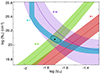	Fig. 8. Same is Fig. 6, using the MF87 SED and solar abundances.
In the text

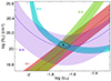	Fig. 9. Same is Fig. 6, using the UV-soft SED and solar abundances.
In the text

	Fig. 10. Excited state (E = 174.4 cm−1) to resonance state column density ratio of N III vs. the electron number density (blue curve) from the Chianti atomic database for T = 16 000 K. The measured ratio is shown by the red dot, and the accompanying error bars are shown by the vertical red lines. The 174.4 cm−1 transition in N III arises from the 2P3/2  →  2P1/2 transition within this ion.
In the text

References

- Arav, N., Korista, K. T., de Kool, M., Junkkarinen, V. T., & Begelman, M. C. 1999a, ApJ, 516, 27 [NASA ADS] [CrossRef] [Google Scholar]
- Arav, N., Becker, R. H., Laurent-Muehleisen, S. A., et al. 1999b, ApJ, 524, 566 [NASA ADS] [CrossRef] [Google Scholar]
- Arav, N., Brotherton, M. S., Becker, R. H., et al. 2001, ApJ, 546, 140 [NASA ADS] [CrossRef] [Google Scholar]
- Arav, N., Kaastra, J., Kriss, G. A., et al. 2005, ApJ, 620, 665 [CrossRef] [Google Scholar]
- Arav, N., Gabel, J. R., Korista, K. T., et al. 2007, ApJ, 658, 829 [NASA ADS] [CrossRef] [Google Scholar]
- Arav, N., Borguet, B., Chamberlain, C., Edmonds, D., & Danforth, C. 2013, MNRAS, 436, 3286 [NASA ADS] [CrossRef] [Google Scholar]
- Arav, N., Xu, X., Kriss, G. A., et al. 2020, A&A, 633, A61 [NASA ADS] [EDP Sciences] [Google Scholar]
- Astropy Collaboration (Robitaille, T. P., et al.) 2013, A&A, 558, A33 [NASA ADS] [CrossRef] [EDP Sciences] [Google Scholar]
- Astropy Collaboration (Price-Whelan, A. M., et al.) 2018, AJ, 156, 123 [Google Scholar]
- Barlow, T. A., Hamann, F., & Sargent, W. L. W. 1997, ASPC, 128, 13 [NASA ADS] [Google Scholar]
- Borguet, B. C. J., Edmonds, D., Arav, N., Dunn, J., & Kriss, G. A. 2012a, ApJ, 751, 107 [CrossRef] [Google Scholar]
- Borguet, B. C. J., Edmonds, D., Arav, N., et al. 2012b, ApJ, 758, 69 [NASA ADS] [CrossRef] [Google Scholar]
- Byun, D., Arav, N., & Walker, A. 2022a, MNRAS, 516, 100 [NASA ADS] [CrossRef] [Google Scholar]
- Byun, D., Arav, N., & Hall, P. B. 2022b, MNRAS, 517, 1048 [NASA ADS] [CrossRef] [Google Scholar]
- Byun, D., Arav, N., & Hall, P. B. 2022c, ApJ, 927, 176 [NASA ADS] [CrossRef] [Google Scholar]
- de Diego, J. A., Binette, L., Ogle, P., et al. 2007, A&A, 467, L7 [NASA ADS] [CrossRef] [EDP Sciences] [Google Scholar]
- Dehghanian, M., Arav, N., Byun, D., et al. 2024, MNRAS, 527, 7825 [Google Scholar]
- de Kool, M., Korista, K. T., & Arav, N. 2002, ApJ, 580, 54 [NASA ADS] [CrossRef] [Google Scholar]
- Dere, K. P., Landi, E., Mason, H. E., Monsignori, Fossi B. C., & Young P. R., 1997, A&AS, 125, 149 [NASA ADS] [CrossRef] [EDP Sciences] [Google Scholar]
- Dere, K. P., Del Zanna, G., Young, P. R., Landi, E., & Sutherland, R. S. 2019, ApJS, 241, 22 [Google Scholar]
- Dunn, J. P., Bautista, M., Arav, N., et al. 2010, ApJ, 709, 611 [NASA ADS] [CrossRef] [Google Scholar]
- Fields, D. L., Mathur, S., Pogge, R. W., et al. 2005, ApJ, 634, 928 [CrossRef] [Google Scholar]
- Floris, A., Marziani, P., Panda, S., et al. 2024, A&A, 689, A321 [NASA ADS] [CrossRef] [EDP Sciences] [Google Scholar]
- Gabel, J. R., Crenshaw, D. M., Kraemer, S. B., et al. 2003, ApJ, 583, 178 [NASA ADS] [CrossRef] [Google Scholar]
- Gabel, J. R., Arav, N., & Kim, T.-S. 2006, ApJ, 646, 742 [NASA ADS] [CrossRef] [Google Scholar]
- Grevesse, N., Asplund, M., Sauval, A. J., et al. 2010, Ap&SS, 328, 179 [NASA ADS] [CrossRef] [Google Scholar]
- Gunasekera, C. M., van Hoof, P. A. M., Chatzikos, M., et al. 2023, Res. Notes Am. Astron. Soc., 7, 246 [Google Scholar]
- Hamann, F. 1996, HST Proposal, 6589 [Google Scholar]
- Hamann, F. 1998, ApJ, 500, 798 [NASA ADS] [CrossRef] [Google Scholar]
- Harris, C. R., Millman, K. J., van der Walt, S. J., et al. 2020, Natur, 585, 357 [NASA ADS] [CrossRef] [Google Scholar]
- He, Z., Liu, G., Wang, T., et al. 2022, Sci. Adv., 8, eabk3291 [NASA ADS] [CrossRef] [Google Scholar]
- Hunter, J. D. 2007, Comput. Sci. Eng., 9, 90 [NASA ADS] [CrossRef] [Google Scholar]
- Itoh, D., Misawa, T., Horiuchi, T., & Aoki, K. 2020, MNRAS, 499, 3094 [NASA ADS] [CrossRef] [Google Scholar]
- Marziani, P., Panda, S., Deconto Machado, A., et al. 2023, Galaxies, 11, 52 [NASA ADS] [CrossRef] [Google Scholar]
- Mathews, W. G., & Ferland, G. J. 1987, ApJ, 323, 456 [NASA ADS] [CrossRef] [Google Scholar]
- Osterbrock, D. E., & Ferland, G. J. 2006, Astrophysics of gaseous nebulae and active galactic nuclei, eds. D. E. Osterbrock & G. J. Ferland (Sausalito, CA: University Science Books) [Google Scholar]
- Planck Collaboration VI. 2020, A&A, 641, A6 [NASA ADS] [CrossRef] [EDP Sciences] [Google Scholar]
- Punsly, B., Marziani, P., Bennert, V. N., et al. 2018, ApJ, 869, 143 [Google Scholar]
- Punsly, B., Groeneveld, C., Hill, G. J., et al. 2022, AJ, 163, 194 [Google Scholar]
- Reback, J., McKinney, W., jbrockmendel, et al. 2021, https://doi.org/10.5281/zenodo.5774815 [Google Scholar]
- Savage, B. D., & Sembach, K. R. 1991, ApJ, 379, 245 [NASA ADS] [CrossRef] [Google Scholar]
- Scannapieco, E., & Oh, S. P. 2004, ApJ, 608, 62 [NASA ADS] [CrossRef] [Google Scholar]
- Silk, J., & Rees, M. J. 1998, A&A, 331, L1 [NASA ADS] [Google Scholar]
- Spitzer, L. 1968, Diffuse Matter in Space (New York: Interscience Publication) [Google Scholar]
- Vayner, A., Wright, S. A., Murray, N., et al. 2021, ApJ, 919, 122 [CrossRef] [Google Scholar]
- Vestergaard, M. 2003, ApJ, 599, 116 [NASA ADS] [CrossRef] [Google Scholar]
- Villar-Martin, M., López Cobá, C., Cazzoli, S., et al. 2024, A&A, 690, A397 [Google Scholar]
- Virtanen, P., Gommers, R., Oliphant, T. E., et al. 2020, Nat. Methods, 17, 261 [Google Scholar]
- Walker, A., Arav, N., & Byun, D. 2022, MNRAS, 516, 3778 [NASA ADS] [CrossRef] [Google Scholar]
- Xu, X., Arav, N., Miller, T., & Benn, C. 2019, ApJ, 876, 105 [NASA ADS] [CrossRef] [Google Scholar]
- Yuan, F., Yoon, D., Li, Y.-P., et al. 2018, ApJ, 857, 121 [Google Scholar]