| Issue |
A&A
Volume 695, March 2025
|
|
|---|---|---|
| Article Number | A4 | |
| Number of page(s) | 7 | |
| Section | Astrophysical processes | |
| DOI | https://doi.org/10.1051/0004-6361/202453384 | |
| Published online | 26 February 2025 | |
An energetic absorption outflow in QSO J1402+2330: Analysis of DESI observations
1
Department of Physics and Astronomy, The University of Kentucky, Lexington, KY 40506, USA
2
Department of Physics, Virginia Tech, Blacksburg, VA 24061, USA
⋆ Corresponding author; This email address is being protected from spambots. You need JavaScript enabled to view it.
Received:
10
December
2024
Accepted:
29
January
2025
Abstract
Context. Quasar outflows play a significant role in the active galactic nucleus (AGN) feedback, impacting the interstellar medium and potentially influencing galaxy evolution. Characterizing these outflows is essential for understanding AGN-driven processes.
Aims. We aim to analyze the physical properties of the mini-broad absorption line outflow in quasar J1402+2330 using data from the Dark Energy Spectroscopic Instrument (DESI) survey. We seek to measure the outflow’s location, energetics, and potential impact on AGN feedback processes.
Methods. In the spectrum of J1402+2330, we identify multiple ionic absorption lines, including ground and excited states. We measure the ionic column densities and then use photoionization models to determine the total hydrogen column density and ionization parameter of the outflow. We utilized the population ratio of the excited state to the ground state of N III and S IV to determine the electron number density.
Results. The derived electron number density, combined with the ionization parameter, indicates an outflow distance of approximately 2.2 kpc from the central source. Having a mass outflow rate of more than one thousand solar masses per year and a kinetic energy output exceeding 5% of the Eddington luminosity, this outflow can significantly contribute to AGN feedback.
Conclusions. Our findings suggest the absorption outflow in J1402+2330 plays a potentially significant role in AGN feedback processes. This study highlights the value of DESI data in exploring AGN feedback mechanisms.
Key words: galaxies: active / galaxies: general / galaxies: individual: J1402+2330 / quasars: absorption lines
© The Authors 2025
 Open Access article, published by EDP Sciences, under the terms of the Creative Commons Attribution License (https://creativecommons.org/licenses/by/4.0), which permits unrestricted use, distribution, and reproduction in any medium, provided the original work is properly cited.
This article is published in open access under the Subscribe to Open model. This email address is being protected from spambots. You need JavaScript enabled to view it. to support open access publication.
1. Introduction
Quasar outflows are invoked as key contributors to active galactic nuclei (AGN) feedback (e.g., Silk & Rees 1998; Scannapieco & Oh 2004; Yuan et al. 2018; Vayner et al. 2021; He et al. 2022). Absorption outflows observed in rest-frame UV spectra are generally classified into broad absorption lines (BALs, ≥2000 km s−1), narrow absorption lines (NALs, ≤500 km s−1), and mini-BALs. Mini-BALs exhibit absorption features with intermediate widths between NALs and traditional BALs, with smooth BAL-like profiles but velocity widths ≤2000 km s−1 (Weymann et al. 1991; Churchill et al. 1999; Hamann & Sabra 2004; Itoh et al. 2020; Hamann et al. 2013). Mini-BAL trough are typically unblended, allowing for reliable determination of ionic column densities. As a result, mini-BALs serve as effective probes of the physical conditions within outflows (Ganguly & Brotherton 2008; Dehghanian et al. 2024, 2025).
The Dark Energy Spectroscopic Instrument (DESI) is a cutting-edge, multi-object spectrograph designed to map the large-scale structure of the universe with remarkable precision. Installed on the Mayall 4-meter telescope at Kitt Peak National Observatory, DESI can observe over 5000 targets simultaneously, enabling the measurement of redshifts for millions of galaxies and quasars across a vast area of the sky. As of June 2023, DESI has identified approximately 90 000 quasars in its Early Data Release (EDR, DESI Collaboration 2024), representing about 2% of its planned survey, which aims to map over 35 million galaxies and quasars (From DESI lab1). The EDR serves as a valuable resource for the scientific community to evaluate DESI’s data quality, calibration, and potential for preliminary cosmological analyses.
Recently, some studies have utilized DESI data to detect and investigate the absorption lines. For instance, Napolitano et al. (2023) detected Mg II (λ2796.28 Å) absorbers via developing an autonomous supplementary spectral pipeline. This was followed by searching for other common metal lines, such as Fe II, C IV, and Si IV. In another study, Filbert et al. (2024) present a catalog of BAL quasars identified in the DESI-EDR survey. The current paper marks the first instance of employing DESI data to analyze the energetics of an absorption outflow system. In this study, we investigate the quasar SDSS J1402+2330, in which two distinct absorption outflow systems are detected. Using DESI spectra, we aim to:
-
Measure the physical parameters of the low-velocity outflow, including ionic column densities (Nion), total hydrogen column density (NH), ionization parameter (UH), electron number density (ne), and distance from the AGN (R).
-
Determine the outflow’s energetics, including the mass-loss-rate and kinetic luminosity, to assess its possible role in AGN feedback.
The paper’s structure is as follows: In Section 2, we describe the observations and data acquisition of the target. Section 3 details the approaches used to calculate Nion of the mini-BALs. From these Nion, we derive the photoionization solution, ne and R. We then calculate the black hole (BH) mass and the quasar’s Eddington luminosity. These are followed by deriving the energetics of the outflow system. Section 4 presents the summary of the paper and concludes it.
Here we adopt standard ΛCDM cosmology with h = 0.677, Ωm = 0.310, and ΩΛ = 0.690 (Planck Collaboration VI 2020). We used the Python astronomy package Astropy (Astropy Collaboration 2013, 2018) for our cosmological calculations, as well as Scipy (Virtanen et al. 2020), Numpy (Harris et al. 2020), and Pandas (Reback et al. 2021) for most of our numerical computations. For our plotting purposes, we used Matplotlib (Hunter 2007).
2. Observation
Quasar SDSS J1402+2330 (hereafter J1402) is a bright quasar, at Redshift z = 2.8302 (based on the NASA/IPAC Extragalactic Database)2, with J2000 coordinates at RA = 14:2:21.52 and Dec =+23:30:43.32. Observations of J1402 were conducted as part of the DESI-EDR survey over two nights: March 10, 2021, and April 4, 2021, with a total exposure time of 5769.5 seconds. The spectral data span the wavelength range of 3600–9800 Å, with a spectral resolution which falls between R ≈ 2000–5000, depending on the specific wavelength observed. The observations are part of the sv1 Survey Validation Phase and were processed with the DESI pipeline, and co-added spectra are referenced in file 3851 from the DESI archive.
After obtaining the data using client developed by SPectra Analysis and Retrievable Catalog Lab (SPARCL), we identified two absorption line outflow systems from multiple ions (see Figure 1):
-
Low-velocity outflow: vcentroid ≈ −4300 km s−1
-
High-velocity outflow: vcentroid ≈ −8500 km s−1
The low-velocity outflow system is the focus of our analysis due to the detection of ground-state and excited-state absorption troughs in its spectrum, including N III, NIII*, S IV, SIV*, C II, and CII* (see Figure 1). The presence of multiple ions in various energy states makes this outflow an especially valuable target for determining its energetics. This outflow has a centroid velocity of approximately vcentroid ≈ −4300 km s−1 and exhibits absorption troughs from Al II, Al III, and P V as well. The absorption width of this system is around 600 km s−1, which categorizes it as a mini-BAL. Throughout this paper, we refer to this high-velocity mini-BAL system as “the outflow.”
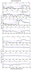 |
Fig. 1. Spectrum of SDSS J1402+2330 as observed by the DESI in 2021. The absorption features of the outflow system with a velocity of −8500 km s−1 are marked with magenta lines, while the green lines show the absorption from the outflow system with a centroid velocity of −4300 km s−1. The dashed blue line shows our continuum emission model. |
The high-velocity absorption outflow is excluded from analysis because reliable column density measurements cannot be obtained for the excited states identified in this system: Both SIV* and NIII* are saturated, and CII* is heavily blended, precluding a reliable assessment.
3. Analysis
Figure 1 displays the spectrum along with the identified absorption lines. As noted above, we focus on the low-velocity outflow system, for which the absorption lines are shown with vertical blue lines (high-redshift).
We exclude O VI doublet (λλ1031.91,1037.61 Å), N V doublet (λλ1238.82, 1242.80 Å), and also Si IV doublet (λλ1393.76, 1402.77 Å) from our analysis, as their flux values approach zero, indicating saturation. Note that the spectrum has a velocity resolution ranging between 60 to 150 km s−1, with the velocity resolution around ∼150 km s−1 at the N III region.
To identify the troughs in the spectrum and determine their ionic column densities, we first obtain a normalized spectrum by dividing the data by the unabsorbed emission model. In the spectrum of J1402, we modeled the unabsorbed emission model with a single power law (Fλ = 6.2E– with λ0 = 1350 Å), while emission regions are modeled with one or more Gaussian functions. Figure 2 presents the normalized flux versus velocity for some of the blue-shifted absorption lines detected in the spectrum of J1402. As shown in the figure, for most of the ions we integrate over a velocity range of −4600 to −4000 km s−1 (width = 600 km s−1). However, for S IV, SIV*, C II, CII*, and Al III the integration range is adjusted to −4400 to −4150 km s−1 to account for differences in absorption features: the regions outside this narrower range deviate from the profile of other absorption troughs and are therefore deemed unreliable for calculations. For P V, the blue trough is excluded due to contamination by the Lyα forest, and the integration range for the red trough is similarly constrained to −4400 to −4150 km s−1.
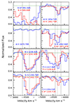 |
Fig. 2. Normalized flux versus velocity for outflow’s absorption troughs detected in the spectrum of J1402. The horizontal green dashed line shows the continuum level, and the vertical black dashed lines show the integration range (see text). The vertical solid gray line indicates the centroid velocity. |
3.1. Determining the ionic column densities
To understand the physical characteristics of the outflow, we start by determining the individual Nion of the absorption troughs. One approach to determine the ionic column densities is the “apparent optical depth” (AOD) method, which assumes that the source is uniformly and completely covered by the outflow (Spitzer 1968; Savage & Sembach 1991). In this scenario, the column densities are determined using Equations (1) and (2) below (e.g., Spitzer 1968; Savage & Sembach 1991; Arav et al. 2001):
 (1)
(1)
![Mathematical equation: $$ \begin{aligned} N_{\text{ ion}}&=\frac{3.77\times 10^{14}}{\lambda _{0}f}\times \int \tau (v)~dv \,[\text{ cm}^{-2}], \end{aligned} $$](/articles/aa/full_html/2025/03/aa53384-24/aa53384-24-eq3.gif) (2)
(2)
where I(v) is the normalized intensity profile as a function of velocity and τ(v) is the optical depth of the absorption trough. λ0 refers to the transition’s wavelength, f is the oscillator strength of the transition, and and v is measured in km s−1. To determine Nion of the S IV and SIV*, we opted for the AOD technique, as they arise from different energy levels and are not saturated, since they are much shallower than the saturated troughs like O VI. Since the absorption troughs of these ions are not very deep, these can be assumed to be unsaturated, and their column density measurements via the AOD method are reliable. For P V, we focus exclusively on its red trough (λ1128.00 Å) and treat it as a singlet. This is because the blue trough is clearly contaminated by Lyα forest absorption (see Figure 2). We are unable to directly apply the AOD method to N III and NIII* absorption troughs, since they are blended (see Figure 2). Instead, we model each ion with a Gaussian function in flux space, ensuring both Gaussians share the same centroid velocity (vcentroid) and width (see Figure 3). We then apply the AOD method to each Gaussian individually and sum the results to determine the final N III ionic column density. For more details regarding the AOD method, see Arav et al. (2001), Gabel et al. (2003), and Byun et al. (2022a).
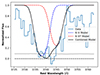 |
Fig. 3. Gaussian modeling of the NIII*λ991.58 Å (blue dashed line) and N IIIλ989.80 Å (red dashed line) absorption troughs. The black solid line shows the final model, which results from combining two Gaussian curves. The grey line shows the level of noise around the modeled region. |
The partial covering (PC) method is applied when two or more lines originate from the same energy level. This method assumes that the outflow partially covers a homogeneous source (Barlow et al. 1997; Arav et al. 1999a,b). In this method, since a velocity-dependent covering factor is determined, the effects of non-black saturation (de Kool et al. 2002) are considered. To use the PC method, we calculate the covering fraction C(v) and optical depth τ(v) using Equations (3) and (4) (see Arav et al. 2005). For doublet transitions, where the blue component has twice the oscillator strength of the red component:
![Mathematical equation: $$ \begin{aligned} I_R(v)-[1-C(v)]=C(v)e^{-\tau (v)} \end{aligned} $$](/articles/aa/full_html/2025/03/aa53384-24/aa53384-24-eq4.gif) (3)
(3)
and
![Mathematical equation: $$ \begin{aligned} I_B(v)-[1-C(v)]=C(v)e^{-2\tau (v)}. \end{aligned} $$](/articles/aa/full_html/2025/03/aa53384-24/aa53384-24-eq5.gif) (4)
(4)
In the equations above, IR(v) and IB(v) are the normalized intensities of the red and blue absorption features, respectively. τ(v) is the optical depth profile of the red component. In this study, we apply the PC method to the Al III doublet (λλ1854.71, 1862.78 Å) since they are both originating from the ground state. We model each trough with a Gaussian in flux space, where both Gaussian functions have the same centroid velocity (vcentroid) and width (see Figure 4). This enables us to calculate the values of τ(v) and C(v). We then use the resultant values in the PC method equations to calculate the column density of Al III. See Barlow et al. (1997), Arav et al. (1999a,b, 2005), de Kool et al. (2002), Borguet et al. (2012), Byun et al. (2022a,b) to find detailed explanations of both methods.
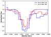 |
Fig. 4. Gaussian modeling of the Al IIIλ1854.72 Å (blue) and the Al IIIλ1862.79 (red) absorption troughs. In both cases, the data are shown in histograms while the fits are shown with dashed lines of the same color. |
We also consider the systematic errors arising from the choice of the continuum (See Figure 4 of Dehghanian et al. 2025). To include this source of error in our calculations, we assume a 10% systematic error. The final adopted errors for ionic column densities are determined by quadratically combining the AOD errors with the 10% systematic uncertainty in the local continuum level. For N III and Al III, the errors derived from the Gaussian fits are quadratically added to the assumed systematic error. Table 1 summarizes the final results of our Nion measurements, along with their associated uncertainties. In this table, two ions are treated as upper limits rather than accurate measurements: SIV*, due to contamination by the Lyα forest, and Al II, as its absorption trough is almost undetectable (see Figures 1 and 2).
Ionic column densities.
3.2. Photoionization modeling
The gas in quasar outflows is in photoionization equilibrium, where the balance between ionization and recombination processes determines the ionization state of the medium (Davidson & Netzer 1979; Krolik 1999; Osterbrock & Ferland 2006, and references therein). Photoionization modeling provides a framework for interpreting the Nion observed in the outflowing gas, allowing us to constrain its physical properties. To achieve this, we use the spectral synthesis code Cloudy (Gunasekera et al. 2023), in combination with the measured Nion to estimate NH and UH of the outflow. Cloudy solves the equations of photoionization equilibrium in the outflow, which we model as a plane-parallel slab with constant hydrogen number density and abundances, ionized by a specified spectral energy distribution (SED). In this approach, we use Cloudy to produce photoionization models that predict all Nion values for a grid of NH and UH values. We then compare these produced Nion to the observed ones to find the NH and UH values that best reproduce the observed Nion. This methodology is the same as was used in previous studies (e.g., Byun et al. 2022a,b,c; Walker et al. 2022; Dehghanian et al. 2024, 2025; Sharma et al. 2024).
Note that the photoionization state of an outflow depends on the assumed abundances and the SED incident upon it. To consider these effects, we explored three SEDs, including HE0238 (Arav et al. 2013), MF87 (Mathews & Ferland 1987), and UV-Soft SED (Dunn et al. 2010), and two sets of abundances: solar (Z = Z⊙) and super-solar metallicity (Z = 4.68 × Z⊙) (Ballero et al. 2008), a total of six models (See Figure 5 of Dehghanian et al. (2025) for a visual comparison of the three SEDs. The accompanying discussion in the text provides further insights into the characteristics of these SEDs). The hydrogen column densities, ionization parameters, and the reduced χ2 resulting from these models are presented in Table 2. We select the UV-soft SED with solar metalicity as our preferred model since this SED is more appropriate to be used for high-luminosity quasars (Dunn et al. 2010), compared to MF87 (which has the same  when paired with super-solar metalicity). Figure 5, upper panel, shows the photoionization modeling using the UV-soft SED and solar metallicity. In this figure, the solid lines show the Nion taken as measurements, while shaded bands are the uncertainties associated with these measurements (see Table 1). The green dotted line indicates that the ionic column density of that specific ion (Al II) is considered to be an upper limit. The black dot shows the best χ2-minimization solution. The lower panel of Figure 5 compares all six models. In this panel, the dots surrounded by the solid-line ovals show the best solution when using each SED and solar metallicity, while the dots surrounded by the dashed-line ovals show the best solution when using each SED and super-solar metallicity.
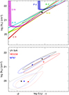 |
Fig. 5. Phase plot showing the photoionization solution. Top: shows the solution for the absorption low-velocity outflow system in J1402, using the UV-soft SED and solar abundances. Each solid line represents the range of models (UH and NH) that predict a column density matching the observed value for that ion. The shaded bands are the uncertainties associated with each Nion measurement. The dotted line (Al II) represents an upper limit. The black dot shows the solution, which is surrounded by χ2, as the black oval. Bottom: solution for a total of six models, including three SEDs (HE0238, MF87, and UV-soft) and two abundances: solar (shown with solid lines) and super-solar (shown with dashed lines). |
3.3. Electron number density
Assuming collisional excitation, we can determine ne of the outflow (see Arav et al. 2018) using the population ratio of excited and ground states of the N III ion. To do so, we use the Chianti 9.0.1 atomic database (Dere et al. 1997, 2019) to predict the abundance ratios of the excited state to the resonance state for N III as a function of ne. These calculations are affected by the temperature of the outflow. We assume a temperature of 15 000 K, predicted by Cloudy for our best (UH, NH) solution (see Table 2). The blue line in Figure 6 displays the predicted ratio versus ne for N III, while the red line shows the same for S IV. The black dot in both cases has a y-value equal to our measurements of the Nion ratio, resulting in an estimation for ne (x-value). Note that while we accept  ratio as a measurement,
  is an upper limit. This is because SIV* is possibly contaminated by the Lyα forest, making it an upper limit rather than an accurate measurement.
Photoionization solution for six models.
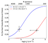 |
Fig. 6. Density diagnostic for the low-velocity absorption outflow. The measured |


To estimate the uncertainties on ne, we first calculate the uncertainties in the column density ratio,  (for detailed explanations see Dehghanian et al. 2025). These uncertainties are represented by vertical black lines. Using these values, we derived the corresponding errors in ne, which are shown by horizontal black lines. A similar approach was applied for S IV; however, instead of a lower bound for the electron number density, we included an arrow to indicate that this ratio is indeed an upper limit and the true ne could be any value below this threshold. Therefore, we base our measurement on the
  ratio that yields
  [cm−3], which is consistent with the upper limit acquired from
  ratio (log(ne)≤4.3 [cm−3], see Fig. 6).
The top axis of Figure 6 displays the distance between the outflow and the central source in parsecs. Below, we describe the method used to convert ne into distance.
3.4. Distance of the outflow from the AGN
We can now use the definition of UH (Equation (14.4) from Osterbrock & Ferland 2006) to calculate the distance between the outflow and the AGN(R):
 (5)
(5)
The ionization parameter UH is already determined from the photoionization modeling (see Section 3.2), nH is the hydrogen density which for a highly ionized plasma is estimated to be  (Osterbrock & Ferland 2006). The speed of light is shown by c, and Q(H) (s−1) is the number of hydrogen-ionizing photons emitted by the central object per second. To determine Q(H), we scale the UV-soft SED with the observed continuum flux of J1402 at λobserved = 5010 Å. We use the quasar’s redshift, adopted ΛCDM cosmology, and the scaled SED to obtain the bolometric luminosity and Q(H) (see Byun et al. 2022b,c; Walker et al. 2022):
Following these steps, we obtain Q(H) = 8.12 ± 0.23 × 1056 s−1 and Lbol = 1.20 ± 0.05 × 1047 erg s−1. Using these values, along with nH and UH, we calculated a distance of  pc for the outflow. Note that the uncertainties arise from the uncertainties in the measurements of Q(H), n(e), and U(H). Similarly, we derive the top x-axis in Figure 6. The S IV’s upper limit on ne yields R > 420 pc, consistent with the N III-based measurement.
3.5. BH mass and the Eddington luminosity
Vestergaard & Peterson (2006) show that, assuming that the AGN broad emission line gas is virialized, one can use the C IV emission line to estimate the BH’s mass:
![Mathematical equation: $$ \begin{aligned} \log (M_{\rm BH}({{\text{ C}}{\small { {\text{ IV}}}}}))=\log \left( {\left[\frac{\mathrm{{FWHM}({\text{ C}}{\small {{\text{ IV}}}})}}{1000\,\mathrm {km\,s}^{-1}}\right]^{2}\left[\frac{\lambda L_{\lambda }(1350\,\AA )}{10^{44} \,\mathrm {erg\,s}^{-1}}\right]^{0.53}}\right). \end{aligned} $$](/articles/aa/full_html/2025/03/aa53384-24/aa53384-24-eq31.gif) (6)
(6)
However, the above equation does not consider the blue-shift in the emission line happening due to the presence of outflows or radiation pressure from the central source (e.g. Coatman et al. 2016). Coatman et al. (2017) took this effects into account and revised Equation (6) as below:
![Mathematical equation: $$ \begin{aligned} M_{\rm BH}({\text{ C}}{\small { {\text{ IV}}}}, \mathrm {Corr.})&=10^{6.71}\left[\frac{\mathrm{{FWHM}({\text{ C}}{\small {{\text{ IV}}}}, \mathrm {Corr.)}}}{1000 \,\mathrm {km\,s}^{-1}}\right]^{2}\times \nonumber \\&\quad \qquad \qquad \left[\frac{\lambda L_{\lambda }(1350\,\AA )}{10^{44}\, \mathrm {erg\,s}^{-1}}\right]^{0.53}, \end{aligned} $$](/articles/aa/full_html/2025/03/aa53384-24/aa53384-24-eq32.gif) (7)
(7)
where:
 (8)
(8)
Figure 7 displays the C IV emission line region, along with our modeled emission line profile and continuum level. From this model, we estimate a FWHM of 5600 km s−1 and a C IV blue-shift of almost 1500 km s−1. These calculations yield a BH mass of  M⊙ and
  (erg s−1).
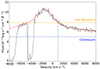 |
Fig. 7. Spectrum in the region around the C IV emission line. The red line shows our total emission model comprised of a continuum fit plus a model for the C IV emission line. The latter is comprised of two Gaussians, one narrow and one broad. The orange line indicates where the half maximum of the emission line model is, while the green dashed lines show the full width of the half maximum. The continuum is subtracted for FWHM determination. We determine a FWHM of 5600 km s−1 and estimate that C IV is blueshifted by about 1500 km s−1. |
3.6. Outflow’s energetics
The mass-loss-rate (̇M) and kinetic luminosity (̇EK) of the outflowing gas can be inferred using the following equations from Borguet et al. (2012):
 (9)
(9)
 (10)
(10)
where μ = 1.4 is the mean atomic mass per proton, v is the outflow’s velocity, and mp is the proton’s mass. Ω is the global covering factor defined as the fraction of the solid angle around the source covered by the outflow. There are several surveys in which C IV BALs are detected in about 20% of all quasars (e.g., Hewett & Foltz 2003; Dai et al. 2012; Gibson et al. 2009; Allen et al. 2011). This detection fraction is usually interpreted to mean that all quasars have BAL outflows with Ω ≈ 0.2, on average. Using the derived values for R, NH, and adopting an Ω of 0.2, for an outflow velocity of −4300 km s−1, we calculate  M⊙ yr−1 and
  [erg s−1]. Note that the uncertainties in the kinetic luminosity are derived from the errors in the ̇M measurement. The errors on ̇M are estimated based on the elliptical shape of the photoionization solution (see Figure. 5), which indicates that the uncertainties in NH and UH are correlated (see Section 4.1 of Walker et al. 2022, for details on error propagation in the ̇M calculation). Based on the values calculated for the bolometric and Eddington luminosities, we find that:

An outflow with a ̇EK/LEdd of at least ≈0.5 % is contributing significantly to the AGN feedback processes (Hopkins & Elvis 2010). The kinetic luminosity of the outflow in J1402 corresponds to more than 5% of the Eddington luminosity, suggesting a strong contribution to AGN feedback processes.
4. Summary and conclusions
In this study, we investigate the properties of a high-energy outflow in quasar J1402+2330, utilizing its spectrum from the DESI survey. While we detect two distinct absorption line outflows, the analysis centers on the low-velocity component due to its rich absorption features, which include ground and excited states from N III, S IV, and C II. Using photoionization modeling and spectral diagnostics, we determine the physical characteristics of the outflow, including electron number density, hydrogen column density, and ionization parameter, which enable us to constrain the outflow’s distance from the central source to approximately 2200 parsecs.
Our results indicate that the outflow has a mass-loss rate on the order of a thousand solar masses per year and a kinetic luminosity that exceeds 5% of the Eddington luminosity. These findings imply that the outflow could play a significant role in AGN feedback, potentially influencing star formation and the interstellar medium within the host galaxy. Table 3 provides a summary of all the physical properties calculated for this outflow system. This work demonstrates the utility of DESI data in resolving the detailed properties of quasar outflows and contributes to our understanding of the broader impact of AGN-driven feedback mechanisms.
Properties of the mini-BAL outflow.
Acknowledgments
We acknowledge support from NSF grant AST 2106249, as well as NASA STScI grants AR-15786, AR-16600, AR- 16601 and AR-17556. This research uses services or data provided by the SPectra Analysis and Retrievable Catalog Lab (SPARCL) and the Astro Data Lab, which are both part of the Community Science and Data Center (CSDC) program at NSF’s National Optical-Infrared Astronomy Research Laboratory. NOIRLab is operated by the Association of Universities for Research in Astronomy (AURA), Inc. under a cooperative agreement with the National Science Foundation.
References
- Allen, J. T., Hewett, P. C., Maddox, N., et al. 2011, MNRAS, 410, 860 [NASA ADS] [CrossRef] [Google Scholar]
- Arav, N., Korista, K. T., de Kool, M., Junkkarinen, V. T., & Begelman, M. C. 1999a, ApJ, 516, 27 [NASA ADS] [CrossRef] [Google Scholar]
- Arav, N., Becker, R. H., Laurent-Muehleisen, S. A., et al. 1999b, ApJ, 524, 566 [NASA ADS] [CrossRef] [Google Scholar]
- Arav, N., Brotherton, M. S., Becker, R. H., et al. 2001, ApJ, 546, 140 [NASA ADS] [CrossRef] [Google Scholar]
- Arav, N., Kaastra, J., Kriss, G. A., et al. 2005, ApJ, 620, 665 [CrossRef] [Google Scholar]
- Arav, N., Borguet, B., Chamberlain, C., Edmonds, D., & Danforth, C. 2013, MNRAS, 436, 3286 [NASA ADS] [CrossRef] [Google Scholar]
- Arav, N., Liu, G., Xu, X., et al. 2018, ApJ, 857, 60 [NASA ADS] [CrossRef] [Google Scholar]
- Astropy Collaboration (Robitaille, T. P., et al.) 2013, A&A, 558, A33 [NASA ADS] [CrossRef] [EDP Sciences] [Google Scholar]
- Astropy Collaboration (Price-Whelan, A. M., et al.) 2018, AJ, 156, 123 [Google Scholar]
- Ballero, S. K., Matteucci, F., Ciotti, L., Calura, F., & Padovani, P. 2008, A&A, 478, 335 [NASA ADS] [CrossRef] [EDP Sciences] [Google Scholar]
- Barlow, T. A., Hamann, F., & Sargent, W. L. W. 1997, ASPC, 128, 13 [NASA ADS] [Google Scholar]
- Borguet, B. C. J., Edmonds, D., Arav, N., Benn, C., & Chamberlain, C. 2012, ApJ, 758, 69 [NASA ADS] [CrossRef] [Google Scholar]
- Byun, D., Arav, N., & Hall, P. B. 2022a, ApJ, 927, 176 [NASA ADS] [CrossRef] [Google Scholar]
- Byun, D., Arav, N., & Hall, P. B. 2022b, MNRAS, 517, 1048 [NASA ADS] [CrossRef] [Google Scholar]
- Byun, D., Arav, N., & Walker, A. 2022c, MNRAS, 516, 100 [NASA ADS] [CrossRef] [Google Scholar]
- Churchill, C. W., Schneider, D. P., Schmidt, M., et al. 1999, AJ, 117, 2573 [NASA ADS] [CrossRef] [Google Scholar]
- Coatman, L., Hewett, P. C., Banerji, M., et al. 2016, MNRAS, 461, 647 [NASA ADS] [CrossRef] [Google Scholar]
- Coatman, L., Hewett, P. C., Banerji, M., et al. 2017, MNRAS, 465, 2120 [Google Scholar]
- Dai, X., Shankar, F., & Sivakoff, G. R. 2012, ApJ, 757, 180 [NASA ADS] [CrossRef] [Google Scholar]
- Davidson, K., & Netzer, H. 1979, Rev. Mod. Phys., 51, 715 [NASA ADS] [CrossRef] [Google Scholar]
- de Kool, M., Korista, K. T., & Arav, N. 2002, ApJ, 580, 54 [NASA ADS] [CrossRef] [Google Scholar]
- Dehghanian, M., Arav, N., Byun, D., et al. 2024, MNRAS, 527, 7825 [Google Scholar]
- Dehghanian, M., Arav, N., Sharma, M., et al. 2025, A&A, 693, A153 [NASA ADS] [CrossRef] [EDP Sciences] [Google Scholar]
- Dere, K. P., Landi, E., Mason, H. E., et al. 1997, A&AS, 125, 149 [NASA ADS] [CrossRef] [EDP Sciences] [Google Scholar]
- Dere, K. P., Del Zanna, G., Young, P. R., Landi, E., & Sutherland, R. S. 2019, ApJS, 241, 22 [Google Scholar]
- DESI Collaboration (Adame, A. G., et al.) 2024, AJ, 168, 58 [NASA ADS] [CrossRef] [Google Scholar]
- Dunn, J. P., Bautista, M., Arav, N., et al. 2010, ApJ, 709, 611 [NASA ADS] [CrossRef] [Google Scholar]
- Filbert, S., Martini, P., Seebaluck, K., et al. 2024, MNRAS, 532, 3669 [NASA ADS] [CrossRef] [Google Scholar]
- Gabel, J. R., Crenshaw, D. M., Kraemer, S. B., et al. 2003, ApJ, 583, 178 [NASA ADS] [CrossRef] [Google Scholar]
- Ganguly, R., & Brotherton, M. S. 2008, ApJ, 672, 102 [CrossRef] [Google Scholar]
- Gibson, R. R., Jiang, L., Brandt, W. N., et al. 2009, ApJ, 692, 758 [Google Scholar]
- Gunasekera, C. M., van Hoof, P. A. M., Chatzikos, M., et al. 2023, Res. Notes Am. Astron. Soc., 7, 246 [Google Scholar]
- Hamann, F., & Sabra, B. 2004, AGN Physics with the Sloan Digital Sky Survey, 311, 203 [NASA ADS] [Google Scholar]
- Hamann, F., Chartas, G., McGraw, S., et al. 2013, MNRAS, 435, 133 [NASA ADS] [CrossRef] [Google Scholar]
- Harris, C. R., Millman, K. J., van der Walt, S. J., et al. 2020, Natur, 585, 357 [NASA ADS] [CrossRef] [Google Scholar]
- He, Z., Liu, G., Wang, T., et al. 2022, Sci. Adv., 8, eabk3291 [NASA ADS] [CrossRef] [Google Scholar]
- Hewett, P. C., & Foltz, C. B. 2003, AJ, 125, 1784 [NASA ADS] [CrossRef] [Google Scholar]
- Hopkins, P. F., & Elvis, M. 2010, MNRAS, 401, 7 [NASA ADS] [CrossRef] [Google Scholar]
- Hunter, J. D. 2007, CSE, 9, 90 [Google Scholar]
- Itoh, D., Misawa, T., Horiuchi, T., & Aoki, K. 2020, MNRAS, 499, 3094 [NASA ADS] [CrossRef] [Google Scholar]
- Krolik, J. H. 1999, Active Galactic Nuclei: from the Central Black Hole to the Galactic Environment, 59 (Princeton University Press) [CrossRef] [Google Scholar]
- Mathews, W. G., & Ferland, G. J. 1987, ApJ, 323, 456 [NASA ADS] [CrossRef] [Google Scholar]
- Miller, T. R., Arav, N., Xu, X., Kriss, G. A., & Plesha, R. J. 2020, ApJS, 247, 39 [NASA ADS] [CrossRef] [Google Scholar]
- Napolitano, L., Pandey, A., Myers, A. D., et al. 2023, AJ, 166, 99 [NASA ADS] [CrossRef] [Google Scholar]
- Osterbrock, D. E., & Ferland, G. J. 2006, Astrophysics of Gaseous Nebulae and Active Galactic Nuclei (Sausalito, CA: University Science Books) [Google Scholar]
- Planck Collaboration VI. 2020, A&A, 641, A6 [NASA ADS] [CrossRef] [EDP Sciences] [Google Scholar]
- Reback, J., McKinney, W., jbrockmendel, et al. 2021, https://doi.org/10.5281/zenodo.4940217 [Google Scholar]
- Savage, B. D., & Sembach, K. R. 1991, ApJ, 379, 245 [NASA ADS] [CrossRef] [Google Scholar]
- Scannapieco, E., & Oh, S. P. 2004, ApJ, 608, 62 [NASA ADS] [CrossRef] [Google Scholar]
- Sharma, M., Arav, N., Zhao, Q., Dehghanian, M., et al. 2024, ApJ, submitted [Google Scholar]
- Silk, J., & Rees, M. J. 1998, A&A, 331, L1 [NASA ADS] [Google Scholar]
- Spitzer, L. 1968, Diffuse Matter in Space (New York: Interscience Publication) [Google Scholar]
- Vayner, A., Wright, S. A., Murray, N., et al. 2021, ApJ, 919, 122 [CrossRef] [Google Scholar]
- Vestergaard, M. 2003, ApJ, 599, 116 [NASA ADS] [CrossRef] [Google Scholar]
- Vestergaard, M., & Peterson, B. M. 2006, ApJ, 641, 689 [Google Scholar]
- Virtanen, P., Gommers, R., Oliphant, T. E., et al. 2020, NatMe, 17, 261 [NASA ADS] [Google Scholar]
- Walker, A., Arav, N., & Byun, D. 2022, MNRAS, 516, 3778 [NASA ADS] [CrossRef] [Google Scholar]
- Weymann, R. J., Morris, S. L., Foltz, C. B., et al. 1991, ApJ, 373, 23 [NASA ADS] [CrossRef] [Google Scholar]
- Yuan, F., Yoon, D., Li, Y.-P., et al. 2018, ApJ, 857, 121 [Google Scholar]
All Tables
All Figures
|
Fig. 1. Spectrum of SDSS J1402+2330 as observed by the DESI in 2021. The absorption features of the outflow system with a velocity of −8500 km s−1 are marked with magenta lines, while the green lines show the absorption from the outflow system with a centroid velocity of −4300 km s−1. The dashed blue line shows our continuum emission model. |
| In the text | |
|
Fig. 2. Normalized flux versus velocity for outflow’s absorption troughs detected in the spectrum of J1402. The horizontal green dashed line shows the continuum level, and the vertical black dashed lines show the integration range (see text). The vertical solid gray line indicates the centroid velocity. |
| In the text | |
|
Fig. 3. Gaussian modeling of the NIII*λ991.58 Å (blue dashed line) and N IIIλ989.80 Å (red dashed line) absorption troughs. The black solid line shows the final model, which results from combining two Gaussian curves. The grey line shows the level of noise around the modeled region. |
| In the text | |
|
Fig. 4. Gaussian modeling of the Al IIIλ1854.72 Å (blue) and the Al IIIλ1862.79 (red) absorption troughs. In both cases, the data are shown in histograms while the fits are shown with dashed lines of the same color. |
| In the text | |
|
Fig. 5. Phase plot showing the photoionization solution. Top: shows the solution for the absorption low-velocity outflow system in J1402, using the UV-soft SED and solar abundances. Each solid line represents the range of models (UH and NH) that predict a column density matching the observed value for that ion. The shaded bands are the uncertainties associated with each Nion measurement. The dotted line (Al II) represents an upper limit. The black dot shows the solution, which is surrounded by χ2, as the black oval. Bottom: solution for a total of six models, including three SEDs (HE0238, MF87, and UV-soft) and two abundances: solar (shown with solid lines) and super-solar (shown with dashed lines). |
| In the text | |
|
Fig. 6. Density diagnostic for the low-velocity absorption outflow. The measured |
| In the text | |
|
Fig. 7. Spectrum in the region around the C IV emission line. The red line shows our total emission model comprised of a continuum fit plus a model for the C IV emission line. The latter is comprised of two Gaussians, one narrow and one broad. The orange line indicates where the half maximum of the emission line model is, while the green dashed lines show the full width of the half maximum. The continuum is subtracted for FWHM determination. We determine a FWHM of 5600 km s−1 and estimate that C IV is blueshifted by about 1500 km s−1. |
| In the text | |
Current usage metrics show cumulative count of Article Views (full-text article views including HTML views, PDF and ePub downloads, according to the available data) and Abstracts Views on Vision4Press platform.
Data correspond to usage on the plateform after 2015. The current usage metrics is available 48-96 hours after online publication and is updated daily on week days.
Initial download of the metrics may take a while.