| Issue |
A&A
Volume 684, April 2024
|
|
|---|---|---|
| Article Number | A158 | |
| Number of page(s) | 7 | |
| Section | Extragalactic astronomy | |
| DOI | https://doi.org/10.1051/0004-6361/202348215 | |
| Published online | 17 April 2024 | |
Extreme FeLoBAL outflow in the VLT/UVES spectrum of quasar SDSS J1321−0041
Department of Physics, Virginia Tech, Blacksburg, VA, USA
e-mail: This email address is being protected from spambots. You need JavaScript enabled to view it.
Received:
9
October
2023
Accepted:
9
February
2024
Abstract
Context. Quasar outflows are often analyzed to determine their ability to contribute to active galactic nucleus (AGN) feedback. We identified a broad absorption line (BAL) outflow in the VLT/UVES spectrum of the quasar SDSS J1321−0041. The outflow shows troughs from Fe II, and is thus categorized as an FeLoBAL. This outfow is unusual among the population of FeLoBAL outflows, as it displays C II and Si II BALs.
Aims. Outflow systems require a kinetic luminosity above ∼0.5% of the quasar’s luminosity to contribute to AGN feedback. For this reason, we analyzed the spectrum of J1321−0041 to determine the outflow’s kinetic luminosity, as well as the quasar’s bolometric luminosity.
Methods. We measured the ionic column densities from the absorption troughs in the spectrum and determined the hydrogen column density and ionization parameter using those column densities as our constraints. We also determined the electron number density, ne, based on the ratios between the excited-state and resonance-state column densities of Fe II and Si II. This allowed us to find the distance of the outflow from its central source, as well as its kinetic luminosity.
Results. We determined the kinetic luminosity of the outflow to be 8.4−5.4+13.7 × 1045 erg s−1 and the quasar’s bolometric luminosity to be 1.72 ± 0.13 × 1047 erg s−1, resulting in a ratio of Ėk/LBol = 4.8−3.1+8.0%. We conclude that this outflow has a sufficiently high kinetic luminosity to contribute to AGN feedback.
Key words: galaxies: active / quasars: absorption lines / quasars: individual: SDSS J132139.86−004151.9
© The Authors 2024
 Open Access article, published by EDP Sciences, under the terms of the Creative Commons Attribution License (https://creativecommons.org/licenses/by/4.0), which permits unrestricted use, distribution, and reproduction in any medium, provided the original work is properly cited.
This article is published in open access under the Subscribe to Open model. This email address is being protected from spambots. You need JavaScript enabled to view it. to support open access publication.
1. Introduction
Active galactic nucleus (AGN) feedback is a process in which an AGN affects the evolution of its host galaxy, including the regulation of the star formation rate and the correlation between the black hole and host galaxy mass (e.g., Silk & Rees 1998; Ciotti et al. 2009; King & Muldrew 2016). In quasars, AGN feedback is often attributed to outflows, which are found in ≲40% quasar spectra as blueshifted absorption troughs (e.g., Hewett & Foltz 2003; Dai et al. 2008; Knigge et al. 2008; Vayner et al. 2021; He et al. 2022). Outflow systems require a kinetic luminosity (Ėk) above ∼0.5% of the quasar’s luminosity (Hopkins & Elvis 2010), which Miller et al. (2020a) interpreted to be the Eddington luminosity (LEdd). Outflow analyses have been conducted in past works, reporting quasar outflows with a sufficient value of Ėk (e.g., Chamberlain et al. 2015; Leighly et al. 2018; Miller et al. 2020b; Byun et al. 2022a,b, 2024; Walker et al. 2022).
The process of finding Ėk involves measuring the ionization parameter (UH) and electron number density (ne) of the outflow, which leads to the distance from the central source (R) and mass outflow rate (Ṁ; Borguet et al. 2012b). For the analysis of ionized outflow, the spectral synthesis code CLOUDY (Ferland et al. 2017) can be used to compare measured ionic column densities with simulated values from models created from a range of UH and hydrogen column density (NH) values (e.g., Miller et al. 2020b; Byun et al. 2022c, 2024; Walker et al. 2022). A category of BAL quasars is known as iron low-ionized BAL (FeLoBAL) quasars, due to the identification of Fe II absorption troughs in their spectra. Recent studies of FeLoBALs include (but are not limited to) the study of a powerful FeLoBAL outflow in the quasar SDSS J135246.37+423923.5 (Choi et al. 2020); the analysis of the FeLoBAL quasar Q0059-2735, whose outflow has shown signs of broad Si II absorption (Xu et al. 2021); and a systematic study of the properties of FeLoBAL quasars using spectral synthesis code SimBAL (Choi et al. 2022a,b; Leighly et al. 2022).
We present the analysis of the UVES spectrum of the quasar SDSS J132139.86−004151.9 (hereafter, J1321−0041), which was retrieved from the Spectral Quasar Absorption Database (SQUAD) published by Murphy et al. (2019). The data from SQUAD have 20 times higher spectral resolution than SDSS spectra, therefore lending themselves to a more detailed analysis. We conducted our analysis through the method described above in order to find Ėk and to determine the outflow’s potential ability to contribute to AGN feedback. Similar analyses of quasar outflows have been conducted in past works using spectra from SQUAD (e.g., Byun et al. 2022a,b; Walker et al. 2022).
This paper is structured as follows. Section 2 describes the observation of J1321−0041, as well as our data acquisition process. Section 3 describes the process through which we have found the outflow’s ionic column densities, NH, UH, and ne values. Section 4 presents the resulting energetics parameters R and Ėk. Section 5 discusses the outflow’s potential ability to contribute to AGN feedback and compares it to other outflows that have been analyzed in the past. Section 6 summarizes and concludes the paper. For our analysis, we adopted a cosmology of h = 0.696, Ωm = 0.286, and ΩΛ = 0.714 (Bennett et al. 2014).
2. Observations and data acquisition
J1321−0041 (J2000: RA = 13:21:39.86, Dec: −00:41:51.9, z = 3.119, Hewett & Wild 2010) was observed with VLT/UVES on February 13, 2008, with a total exposure time of 22,800 seconds, as part of program 080.B-0445(A). Murphy et al. (2019) normalized the spectrum by the quasar’s continuum and emission and added it to SQUAD. The quasar was also observed on 4 February 2000, 1 May 2000, and 16 March 2001 as part of the Sloan Digital Sky Survey (SDSS), with little to no time variability between observations. We co-added the SDSS spectra to scale the flux of the UVES spectrum shown in Fig. 1 and to find the bolometric luminosity of the quasar. The co-added SDSS spectrum can be seen in Fig. 2.
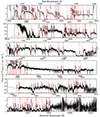 |
Fig. 1. UVES spectrum of J1321−0041. Located absorption troughs and expected locations of absorption troughs from an outflow system, at v ≈ −4100 km s−1, are marked with red vertical lines. The flux has been scaled to match the flux of the SDSS spectrum at observed wavelength λ = 6850 Å. |
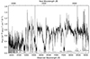 |
Fig. 2. SDSS spectrum of J1321−0041 that was used to scale the continuum flux of the UVES spectrum and to calculate the quasar’s bolometric luminosity. The flux is plotted in black and the error is plotted in gray. |
We have identified broad absorption line (BAL) outflow traveling at v ≈ −4100 km s−1 with troughs of multiple ionic transitions in the UVES spectrum of J1321−0041, including C IV, Si IV, Si II, and Fe II. The velocity of the outflow was determined based on the deepest part of the Si IIλ1808 absorption. The detection of Fe II absorption features puts this outflow in the class of FeLoBALs. The outflow is unusual, as its C II trough by itself adheres to the definition of a BAL (Weymann et al. 1991), as its width is ∼2300 km s−1. Only relatively few such objects are described in the literature (Xu et al. 2021; Choi et al. 2022b). The presence of multiple energy states of Fe II and Si II have enabled us to estimate the outflow’s ne, R, and Ṁ values, and by extension, Ėk. The Fe II* transition lines used for this paper’s analysis, and their associated energies, are shown in Table 1.
Fe II* lines that were used for the ne analysis.
3. Analysis
3.1. Ionic column densities
The first step of our analysis was to find the column densities (Nion) of the ions found in the outflow system. We converted the normalized UVES spectrum from wavelength space to velocity space using the systemic redshift of the quasar (see Fig. 3), and measured the ionic column densities assuming an apparent optical depth (AOD) of a uniform and homogeneously covering outflow (Spitzer 1978; Savage & Sembach 1991).
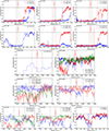 |
Fig. 3. Normalized spectrum of J1321−0041, converted into velocity space. Troughs of individual ionic transitions are color coded, and the integration ranges used for column density calculations are marked by vertical dotted lines. The continuum is represented by a horizontal dashed line. All spectra shown are UVES spectra, except for that of the S IV absorption, which is based on the SDSS spectra due to wavelength range limitations. We note the stark contrast in the signal-to-noise ratio. The bottom three panels show the Fe II and Si II absorption, which were used to estimate ne. |
The AOD method relates the intensity and optical depth as follows:
 (1)
(1)
where I(λ) is intensity as a function of wavelength, I0(λ) is what the intensity would be without absorption, and τ(λ) is the optical depth. Normalizing a spectrum makes the process of finding the optical depth relatively easier, as it becomes a matter of relating the normalized intensity I(λ)/I0(λ) to e−τ(λ). Finding the optical depth allows us to find the column density, as they are related as follows (Spitzer 1978):
 (2)
(2)
where e is elementary charge (C), me is electron mass (kg), f is the oscillator strength of the ionic transition (unitless), λ is the wavelength of the transition (Å), and N(v) is column density per unit velocity (cm−2/km s−1). The column density of an ion can be found by integrating N(v) over the velocity range of the absorption trough. While this is a simple and straightforward method to estimating the ionic column density, it is limited to finding the lower limits when measuring column densities from saturated lines.
We identified the velocity range of the Fe II absorption to be −4200 km s−1 ≲ v ≲ −4000 km s−1 (see bottom panel of Fig. 3) and integrated over that range to find the ionic column densities of the outflow, as shown in Table 2. The red boundary was determined based on the red wing of the deepest absorption trough of Si II. The integration range was kept consistent among the different ions to allow direct comparison of different column densities. The Cr II lines that we identified are those of Cr II* λ1358.71 and λ2161.38. Despite the oscillator strength of the latter being three orders of magnitude larger (f = 0.014 vs. 2.3 × 10⁻⁵), the depth of the former trough is deeper, suggesting that the absorption features may be contaminated (see Fig. 3). Thus, we determined that we would be unable to reliably measure the column density of Cr II. We have identified two visible Co II* troughs, Co II* λ2260 and 2286, from which we have determined a lower limit of Co II column density. We note the reported column densities in Table 2 of ions with multiple energy states, such as Fe II and Ni II, which are the sum of several energy states. The column densities of both Fe II and Ni II are dominated by their resonance states. We also note that the Fe III transitions are marked in Fig. 1 for completion, but they do not have associated discernible troughs. For the photoionization analysis to be described in Sect. 3.2, we added 20% of the column densities to their errors in quadrature to take into account systemic uncertainties, such as that of the modeling of the continuum, following the methodology of Xu et al. (2018). We note that the majority of the adopted values are lower limits, largely due to saturation of the absorption lines.
Ionic column densities of the outflow of J1321−0041.
3.2. Photoionization analysis
We used the spectral synthesis code CLOUDY (Ferland et al. 2017) to find the best fitting values of the hydrogen column density (NH) and the ionization parameter (UH), by comparing modeled values of ionic column densities to the measured values shown in Table 2. Analyses using this method have been carried out in previous works as well (e.g., Byun et al. 2022a; Walker et al. 2022). As shown in Fig. 4, CLOUDY was used to create a grid of outflow models using a range of NH and UH values, with the measured ionic column densities serving as constraints to the parameters. Assuming solar metallicity and the spectral energy distribution (SED) of the quasar HE 0238−1904 (hereafter, HE0238, Arav et al. 2013), this results in the best fitting solution of  and
and  cm−2. The SED of HE0238-1904 is the best empirically determined SED in the extreme UV, which most of the ionizing photons come from (Arav et al. 2013). We note that this solution depends on the assumption that the column density of S IV is a measurement, an assumption we make as we find S IV to be relatively unsaturated. Setting the column density of S IV to be a lower limit results in an unbound lower limit of UH. We note that the S IV trough is from the SDSS spectrum, as it was outside the wavelength range of the SQUAD spectrum.
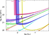 |
Fig. 4. Plot of hydrogen column density (log NH) vs. ionization parameter (log UH), with constraints based on the measured ionic column densities shown in Table 2. Measurements are shown as solid curves, while the dashed curves show lower limits. The colored shades indicate the uncertainties in the constraints of the parameters based on the uncertainties in column density. The black dot shows the solution of log NH and log UH that best matches the column densities, while the black ellipse indicates the 1-σ error. |
3.3. Electron number density
Assuming collisional excitation (an assumption verified by CLOUDY simulations), an outflow’s electron number density can be found from the column density ratios between different energy states of ions (e.g., Moe et al. 2009). We used the troughs of Si II and Fe II that we found to be relatively unsaturated and free of contamination (see bottom panel of Fig. 3) and overlaid the ratios between resonance and excited states of the ions with the relation between column density ratio and ne calculated using the CHIANTI atomic database (version 9.0.1, Dere et al. 1997, 2019). The Si II states were those with energies of E(cm−1) = 0, 287 and those of Fe II had E(cm−1) = 0, 667, 2430, 2837, 3117, 7955. The resulting log ne values ranged from 2.9 to 4.2 (see Fig. 6). We calculated the weighted mean of log ne, following the linear method described by Barlow (2003). For the uncertainty, we used:
 (3)
(3)
where ⟨log ne⟩ is the weighted mean, log ne,ex is the maximum (minimum) measured log ne used when calculating the upper (lower) error, and N is the number of measured log ne values. This resulted in  . We note that the range of log ne values is within 2-σ of the weighted mean.
We were also able to find troughs of Fe II* of energies E = 385, 13 474, 22 637, and 27 620, which had smaller oscillator strengths than the troughs that had been used for this analysis (see Table 3). Despite the smaller oscillator strength values, the troughs are as deep as (or even deeper than) the troughs that have been used for the number density calculation (see bottom panels of Figs. 3 and 5 for comparison). This suggests that the troughs may have been contaminated by unidentified absorption features, making them unreliable indicators of Fe II* column density. Thus, we have excluded them from this calculation.
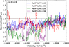 |
Fig. 5. Fe II* absorption troughs that have been excluded from the calculation of log ne. |
Oscillator strengths of Fe II lines found in the spectrum.
4. Results
With NH, UH, and ne found (see Table 4), we could determine the distance of the outflow from the source based on the definition of UH:
 (4)
(4)
Physical parameters of the outflow of J1321−0041.
where QH is the emission rate of Hydrogen ionizing photons, R is the outflow’s distance from the quasar, and nH is the Hydrogen number density. Following the approximation of ne ≈ 1.2nH for highly ionized plasma (Osterbrock & Ferland 2006), we could calculate the value of R once QH was found.
In order to find QH, and by extension, the bolometric luminosity LBol, we scaled the SED of HE0238 to match the continuum flux at observed wavelength λ = 5850 Å, Fλ = 8.25 ± 0.64 × 10⁻¹⁷ erg s−1 cm−2. We then integrated the SED for energies above 1 Ryd, resulting in QH = 9.6 ± 0.7 × 1056 s−1, and LBol = 1.72 ± 0.13 × 1047 erg s−1. The resulting outflow distance was  kpc.
kpc.
5. Discussion
5.1. AGN feedback contribution
An outflow’s kinetic luminosity must be at least ∼0.5% of the quasar’s Eddington luminosity in order to contribute to AGN feedback (Hopkins & Elvis 2010; Miller et al. 2020a). Finding this ratio requires both the kinetic luminosity, Ėk, and Eddington luminosity, LEdd. A quasar’s LEdd value is typically found by measuring the width of an emission feature, such as that of C IV or Mg II, and estimating the mass of the black hole (Vestergaard & Peterson 2006; Coatman et al. 2017; Bahk et al. 2019). However, as can be seen in Fig. 1, the spectrum of J1321−0041 lacks a prominent emission feature which we could use to make such an estimate. Therefore, we used LBol as described in Sect. 4 as a substitute metric, assuming that LEdd ≈ LBol, as this has been the case for several quasars that have been analyzed via this method (e.g., Byun et al. 2022a,b). We advise caution in taking this assumption at face value, as it has shown to not always be the case for FeLoBALQs (e.g., Leighly et al. 2022). We assumed that the geometrical shape of the outflow was that of an incomplete spherical shell, and found the mass flow rate:
 (5)
(5)
where Ω = 0.2 is the global covering factor, μ = 1.4 is the mean atomic mass per proton, mp is proton mass, and v is outflow velocity (Borguet et al. 2012a, 2013). The global covering factor 0.2 is adopted based on the ∼20% ratio of quasars in which C IV BALs are found (Hewett & Foltz 2003). Despite the relative rarity of low-ionized BALs with troughs such as Si II or C II, it is likely that quasars with such LoBALs are BALQSOs at a specific line of sight (see Dunn et al. 2010 for a full discussion). We then calculated the kinetic luminosity ( ), resulting in
  . The ratio between the kinetic luminosity and bolometric luminosity is
  , which would be sufficient to contribute to AGN feedback (see Table 4 for a full summary of the parameters).
5.2. Comparison with other outflows
The nH value of the J1321−0041 outflow was found mainly by examining the ratios between the Fe II excited and resonance state column densities. This has been done in past studies as well (e.g., Dai et al. 2008; Byun et al. 2022c). The ne values from the different ratios agree within ∼0.5 dex with the mean (see Fig. 6) and combined with the previous outflow analyses, this demonstrates that Fe II is an effective probe for nH and outflow distance.
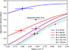 |
Fig. 6. Measured column density ratios of different energy states of Si II and Fe II versus electron number density (log ne), calculated using CHIANTI (Dere et al. 1997, 2019). The color-coded curves are the theoretical relationships between ratio vs. ne, while the dots indicate the measured ratios and associated log ne values. The weighted mean of |
In previous analyses of FeLoBALs based on high resolution VLT/UVES data, the distance R has been measured to be within the range of 1 kpc ≲ R ≲ 67 kpc (e.g., Byun et al. 2022a,c; Walker et al. 2022). The distance of the J1321−0041 outflow from its source is R ≈ 2500 pc, which is well within this range.
As previously mentioned, there have been studies analyzing extreme FeLoBALs in the past. Xu et al. (2021) analyzed the physical conditions of the FeLoBAL of the quasar Q0059−2735, which had a C IV width of ∼25 000 km s−1, roughly twice as wide as the C IV width of J1321−0041 (∼10 000 km s−1) found in its SDSS spectrum. Choi et al. (2022b) studied a larger sample of FeLoBALs, some of which have extreme blending in their absorption troughs. The presence of unblended absorption features in the J1321−0041 spectrum enabled us to conduct a precise analysis of the physical parameters of the outflow system.
6. Summary and conclusion
We have identified an FeLoBAL outflow system in the VLT/UVES spectrum of the quasar SDSS J1321−0041. Through the measurement of ionic column densities and photoionization analysis, we determined the hydrogen column density and ionization parameter of the outflow (see Fig. 4 and Table 4).
The presence of Fe II and Si II absorption trough enabled us to find the electron number density ne by using CHIANTI to relate their column density ratios to estimates of ne. This allowed us to determine the outflows distance from its central source, kinetic luminosity, and the ratio between kinetic luminosity and the quasar’s bolometric luminosity ( ). Assuming LBol ≈ LEdd, the value of Ėk is above the required threshold to contribute to AGN feedback.
Acknowledgments
We acknowledge support from NSF grant AST 2106249, as well as NASA STScI grants AR-15786, AR-16600, and AR-16601.
References
- Arav, N., Borguet, B., Chamberlain, C., Edmonds, D., & Danforth, C. 2013, MNRAS, 436, 3286 [NASA ADS] [CrossRef] [Google Scholar]
- Bahk, H., Woo, J.-H., & Park, D. 2019, ApJ, 875, 50 [NASA ADS] [CrossRef] [Google Scholar]
- Barlow, R. 2003, in Statistical Problems in Particle Physics, Astrophysics, and Cosmology, eds. L. Lyons, R. Mount, & R. Reitmeyer, 250 [Google Scholar]
- Bennett, C. L., Larson, D., Weiland, J. L., & Hinshaw, G. 2014, ApJ, 794, 135 [Google Scholar]
- Borguet, B., Edmonds, D., Arav, N., Dunn, J., & Kriss, G. A. 2012a, ApJ, 751, 107 [CrossRef] [Google Scholar]
- Borguet, B. C. J., Edmonds, D., Arav, N., Benn, C., & Chamberlain, C. 2012b, ApJ, 758, 69 [NASA ADS] [CrossRef] [Google Scholar]
- Borguet, B. C. J., Arav, N., Edmonds, D., Chamberlain, C., & Benn, C. 2013, ApJ, 762, 49 [NASA ADS] [CrossRef] [Google Scholar]
- Byun, D., Arav, N., & Hall, P. B. 2022a, ApJ, 927, 176 [NASA ADS] [CrossRef] [Google Scholar]
- Byun, D., Arav, N., & Hall, P. B. 2022b, MNRAS, 517, 1048 [NASA ADS] [CrossRef] [Google Scholar]
- Byun, D., Arav, N., & Walker, A. 2022c, MNRAS, 516, 100 [NASA ADS] [CrossRef] [Google Scholar]
- Byun, D., Arav, N., Dehghanian, M., Walker, G., & Kriss, G. A. 2024, MNRAS, 529, 3550 [NASA ADS] [CrossRef] [Google Scholar]
- Chamberlain, C., Arav, N., & Benn, C. 2015, MNRAS, 450, 1085 [NASA ADS] [CrossRef] [Google Scholar]
- Choi, H., Leighly, K. M., Terndrup, D. M., Gallagher, S. C., & Richards, G. T. 2020, ApJ, 891, 53 [NASA ADS] [CrossRef] [Google Scholar]
- Choi, H., Leighly, K. M., Dabbieri, C., et al. 2022a, ApJ, 936, 110 [NASA ADS] [CrossRef] [Google Scholar]
- Choi, H., Leighly, K. M., Terndrup, D. M., et al. 2022b, ApJ, 937, 74 [NASA ADS] [CrossRef] [Google Scholar]
- Ciotti, L., Ostriker, J. P., & Proga, D. 2009, ApJ, 699, 89 [NASA ADS] [CrossRef] [Google Scholar]
- Coatman, L., Hewett, P. C., Banerji, M., et al. 2017, MNRAS, 465, 2120 [Google Scholar]
- Dai, X., Shankar, F., & Sivakoff, G. R. 2008, ApJ, 672, 108 [NASA ADS] [CrossRef] [Google Scholar]
- Dere, K. P., Landi, E., Mason, H. E., Monsignori Fossi, B. C., & Young, P. R. 1997, A&AS, 125, 149 [NASA ADS] [CrossRef] [EDP Sciences] [Google Scholar]
- Dere, K. P., Zanna, G. D., Young, P. R., Landi, E., & Sutherland, R. S. 2019, ApJS, 241, 22 [CrossRef] [Google Scholar]
- Dunn, J. P., Bautista, M., Arav, N., et al. 2010, ApJ, 709, 611 [NASA ADS] [CrossRef] [Google Scholar]
- Ferland, G. J., Chatzikos, M., Guzmán, F., et al. 2017, Rev. Mex. Astron. Astrofis, 53, 385 [Google Scholar]
- He, Z., Liu, G., Wang, T., et al. 2022, Sci. Adv., 8, eabk3291 [NASA ADS] [CrossRef] [Google Scholar]
- Hewett, P. C., & Foltz, C. B. 2003, AJ, 125, 1784 [NASA ADS] [CrossRef] [Google Scholar]
- Hewett, P. C., & Wild, V. 2010, MNRAS, 405, 2302 [NASA ADS] [Google Scholar]
- Hopkins, P. F., & Elvis, M. 2010, MNRAS, 401, 7 [NASA ADS] [CrossRef] [Google Scholar]
- King, A., & Muldrew, S. I. 2016, MNRAS, 455, 1211 [CrossRef] [Google Scholar]
- Knigge, C., Scaringi, S., Goad, M. R., & Cottis, C. E. 2008, MNRAS, 386, 1426 [NASA ADS] [CrossRef] [Google Scholar]
- Leighly, K. M., Terndrup, D. M., Gallagher, S. C., Richards, G. T., & Dietrich, M. 2018, ApJ, 866, 7 [NASA ADS] [CrossRef] [Google Scholar]
- Leighly, K. M., Choi, H., DeFrancesco, C., et al. 2022, ApJ, 935, 92 [NASA ADS] [CrossRef] [Google Scholar]
- Miller, T. R., Arav, N., Xu, X., & Kriss, G. A. 2020a, MNRAS, 499, 1522 [NASA ADS] [CrossRef] [Google Scholar]
- Miller, T. R., Arav, N., Xu, X., Kriss, G. A., & Plesha, R. J. 2020b, ApJS, 247, 39 [NASA ADS] [CrossRef] [Google Scholar]
- Moe, M., Arav, N., Bautista, M. A., & Korista, K. T. 2009, ApJ, 706, 525 [NASA ADS] [CrossRef] [Google Scholar]
- Murphy, M. T., Kacprzak, G. G., Savorgnan, G. A., & Carswell, R. F. 2019, MNRAS, 482, 3458 [NASA ADS] [CrossRef] [Google Scholar]
- Osterbrock, D. E., & Ferland, G. J. 2006, Astrophysics of Gaseous Nebulae and Active Galactic Nuclei (University Science Books) [Google Scholar]
- Savage, B. D., & Sembach, K. R. 1991, ApJ, 379, 245 [NASA ADS] [CrossRef] [Google Scholar]
- Silk, J., & Rees, M. J. 1998, A&A, 331, L1 [NASA ADS] [Google Scholar]
- Spitzer, L. 1978, Physical Processes in the Interstellar Medium (New York: Wiley) [Google Scholar]
- Vayner, A., Wright, S. A., Murray, N., et al. 2021, ApJ, 919, 122 [CrossRef] [Google Scholar]
- Vestergaard, M., & Peterson, B. M. 2006, ApJ, 641, 689 [Google Scholar]
- Walker, A., Arav, N., & Byun, D. 2022, MNRAS, 516, 3778 [NASA ADS] [CrossRef] [Google Scholar]
- Weymann, R. J., Morris, S. L., Foltz, C. B., & Hewett, P. C. 1991, ApJ, 373, 23 [NASA ADS] [CrossRef] [Google Scholar]
- Xu, X., Arav, N., Miller, T., & Benn, C. 2018, ApJ, 858, 39 [Google Scholar]
- Xu, X., Arav, N., Miller, T., Korista, K. T., & Benn, C. 2021, MNRAS, 506, 2725 [NASA ADS] [CrossRef] [Google Scholar]
All Tables
All Figures
|
Fig. 1. UVES spectrum of J1321−0041. Located absorption troughs and expected locations of absorption troughs from an outflow system, at v ≈ −4100 km s−1, are marked with red vertical lines. The flux has been scaled to match the flux of the SDSS spectrum at observed wavelength λ = 6850 Å. |
| In the text | |
|
Fig. 2. SDSS spectrum of J1321−0041 that was used to scale the continuum flux of the UVES spectrum and to calculate the quasar’s bolometric luminosity. The flux is plotted in black and the error is plotted in gray. |
| In the text | |
|
Fig. 3. Normalized spectrum of J1321−0041, converted into velocity space. Troughs of individual ionic transitions are color coded, and the integration ranges used for column density calculations are marked by vertical dotted lines. The continuum is represented by a horizontal dashed line. All spectra shown are UVES spectra, except for that of the S IV absorption, which is based on the SDSS spectra due to wavelength range limitations. We note the stark contrast in the signal-to-noise ratio. The bottom three panels show the Fe II and Si II absorption, which were used to estimate ne. |
| In the text | |
|
Fig. 4. Plot of hydrogen column density (log NH) vs. ionization parameter (log UH), with constraints based on the measured ionic column densities shown in Table 2. Measurements are shown as solid curves, while the dashed curves show lower limits. The colored shades indicate the uncertainties in the constraints of the parameters based on the uncertainties in column density. The black dot shows the solution of log NH and log UH that best matches the column densities, while the black ellipse indicates the 1-σ error. |
| In the text | |
|
Fig. 5. Fe II* absorption troughs that have been excluded from the calculation of log ne. |
| In the text | |
|
Fig. 6. Measured column density ratios of different energy states of Si II and Fe II versus electron number density (log ne), calculated using CHIANTI (Dere et al. 1997, 2019). The color-coded curves are the theoretical relationships between ratio vs. ne, while the dots indicate the measured ratios and associated log ne values. The weighted mean of |
| In the text | |
Current usage metrics show cumulative count of Article Views (full-text article views including HTML views, PDF and ePub downloads, according to the available data) and Abstracts Views on Vision4Press platform.
Data correspond to usage on the plateform after 2015. The current usage metrics is available 48-96 hours after online publication and is updated daily on week days.
Initial download of the metrics may take a while.