| Issue |
A&A
Volume 693, January 2025
|
|
|---|---|---|
| Article Number | A198 | |
| Number of page(s) | 18 | |
| Section | The Sun and the Heliosphere | |
| DOI | https://doi.org/10.1051/0004-6361/202450945 | |
| Published online | 17 January 2025 | |
Electron and proton peak intensities as observed by a five-spacecraft fleet in solar cycle 25
1
Department of Physics and Astronomy, 20014 University of Turku, Finland
2
Heliophysics Science Division, NASA Goddard Space Flight Center, Greenbelt, MD 20771, USA
3
Department of Astronomy, University of Maryland, College Park, MD 20742, USA
4
Institute of Experimental and Applied Physics, Kiel University, Kiel, Germany
5
European Space Agency (ESA), European Space Astronomy Centre (ESAC), Camino Bajo del Castillo s/n, 28692 Villanueva de la Cañada, Madrid, Spain
6
Universidad de Alcalá, Space Research Group (SRG-UAH), Plaza de San Diego s/n, 28801 Alcalá de Henares, Madrid, Spain
⋆ Corresponding author; This email address is being protected from spambots. You need JavaScript enabled to view it.
Received:
31
May
2024
Accepted:
28
October
2024
Abstract
Context. Solar energetic particle (SEP) events are related to solar flares and fast coronal mass ejections (CMEs). In the case of large events, which are typically associated with both a strong flare and a fast CME driving a shock front, identification of the dominant SEP acceleration mechanism is challenging.
Aims. Using novel spacecraft observations of strong SEP events detected in solar cycle 25, we aim to identify the parent acceleration region of the observed electron and proton events.
Methods. We analysed 45 SEP events in November 2020 – May 2023 including > 25 MeV protons using data from multiple spacecraft, including Solar Orbiter, near-Earth spacecraft (SOHO and Wind), STEREO A, BepiColombo, and Parker Solar Probe. We used peak intensities of 25–40 MeV protons and ∼100 keV and 1 MeV electrons provided by the SERPENTINE multi-spacecraft SEP event catalogue, and studied the correlations between these peak intensities as well as with the intensity of a soft-X-ray flare associated with the SEP event. We also separated the events into those well connected and those poorly connected to the flare by the interplanetary magnetic field.
Results. We find significant correlations between electron and proton peak intensities. While events detected by poorly connected observers show a single population of events, consistent with the idea that these particles are all accelerated by a spatially extended CME-driven shock, events observed in well-connected regions show two populations. One of these populations presents higher proton peak intensities that correlate with electron peak intensities, similarly to the poorly connected events. The other population shows low proton intensities that are less well correlated with electron peak intensities. Based on our findings, we propose that the latter population is a mixture of flare- and shock-accelerated events.
Conclusions. Although this study focuses on relatively energetic SEP events including > 25 MeV protons often attributed to acceleration by CME-driven shocks, we find clear indications of a flare contribution to both electron and proton fluxes in those events originating in sectors magnetically well connected to the source region.
Key words: Sun: coronal mass ejections (CMEs) / Sun: flares / Sun: heliosphere / Sun: particle emission
© The Authors 2025
 Open Access article, published by EDP Sciences, under the terms of the Creative Commons Attribution License (https://creativecommons.org/licenses/by/4.0), which permits unrestricted use, distribution, and reproduction in any medium, provided the original work is properly cited.
This article is published in open access under the Subscribe to Open model. This email address is being protected from spambots. You need JavaScript enabled to view it. to support open access publication.
1. Introduction
Solar energetic particle (SEP) events are major outbursts of energetic charged particle radiation from the Sun. Observations from multiple, widely separated spacecraft provide a powerful tool for investigating particle acceleration and transport mechanisms in large SEP events. The magnetic connection of the observing spacecraft relative to the centre of the solar eruption plays a vital role in determining the observed properties of SEPs (e.g., Richardson et al. 2014; Dresing et al. 2014; Rodríguez-García et al. 2023a). The two main accelerators of SEPs are considered to be solar flares and coronal mass ejection (CME)-driven shock waves (e.g., Reames 2013). The main difference between these accelerators is their size; the flares are small, and so the accelerated particles are expected to only have access to narrow angular regions of the interplanetary magnetic field, while CME-driven shocks represent extended acceleration regions. In strong events that exhibit both a flare and a CME-driven shock, the contributions to the accelerated SEPs can be potentially mixed (e.g., Cane et al. 2003, 2006, based on SEP ion abundances). A shock-related source is expected to dominate SEP events observed at locations that are magnetically poorly connected to the parent active region site, where direct access to the flare source is unlikely. In contrast, SEP events from well-connected regions can potentially contain contributions from both sources; though these contributions may vary for different particle species and energy ranges. Recently, Dresing et al. (2022) suggested that in large and energetic SEP events, relativistic electrons (∼1 MeV) are predominantly accelerated by CME-driven shocks, whereas near-relativistic electrons (∼100 keV) result from a mixture of flare and shock acceleration. This result was corroborated by Rodríguez-García et al. (2023a).
In an earlier study, Cliver & Ling (2007) analysed electron-to-proton peak intensity ratios using a sample of 179 independent SEP events to identify the acceleration mechanism in these events. For that study, SEP events occurring during November 1994 to April 2004 were investigated based only on near-Earth observations. The authors considered peak integral fluxes for > 10 MeV and > 30 MeV protons, and intensities of 0.5 MeV and 4.4 MeV electrons for two groups of events: well-connected events (with associated flares located between W20° and W90°) and poorly connected events (with associated flares within E40° to W19° or W91° to W150°). These authors identified two distinct SEP populations. The first shows low proton peak intensities and higher electron-to-proton peak intensity ratios. This combination of characteristics is only found in well-connected events, and Cliver & Ling (2007) proposed that they are most-likely associated with flare acceleration. The second SEP population shows higher proton peak intensities and lower electron-to-proton ratios, and is presumed to be dominated by shock acceleration in both well- and poorly connected events. The authors reported a negligible and a significant association of type II radio bursts with these respective populations.
In another study, Cane et al. (2010) analysed a set of 340 proton events occurring during 1997–2006 with proton energies of > 25 MeV. The authors examined the distribution of electron-to-proton peak intensity ratios for a subset of 80 events and concluded that the distribution of peak intensity ratios of (∼0.5 MeV) electrons and (∼25 MeV) protons was a continuum of values, without any distinction between relatively electron-rich and electron-poor events. This result supports a single SEP population rather than two distinct populations of electron-rich and electron-poor events. Trottet et al. (2015), based on a sample of 38 SEP events associated with strong flares (class M and X) between 1997 to 2006, reported a strong correlation between the peak intensities of protons with ∼10 MeV energy and near relativistic electrons, suggesting a common acceleration mechanism for electrons and protons. In a recent study, Rodríguez-García et al. (2023a), based on a correlation study of peak intensities of ∼25 keV to ∼1 MeV electrons in 61 solar energetic electron events (SEEs) from 2010 to 2015 observed by the MESSENGER mission, inferred the contribution of both the flare and CME-driven shocks to the acceleration of near-relativistic electrons.
The aim of the present study is to test the results of Cliver & Ling (2007) using a new data set including ∼100 keV electrons, which Dresing et al. (2022) suggested show a stronger relationship with flares than the relativistic electrons considered by Cliver & Ling (2007). In particular, we make use of the multi-spacecraft SEP event catalogue generated as part of the SERPENTINE project (Dresing et al. 2024a,b).
Our analysis is based on studying the correlations between the peak intensities of SEP events using multi-spacecraft observations at different longitudinal locations. Similar to Cliver & Ling (2007), we separated our sample into events where the solar source is well-connected and poorly connected to the observing spacecraft. The poorly connected events are further split into those where the spacecraft connection is east or west relative to the solar source. SEP peak proton and electron intensity correlations are investigated to potentially identify the presence of different SEP populations related with the flare or the shock.
Section 2 introduces the spacecraft and the instruments used, as well as the classification of events and analysis methods. The results of the study are presented in Sect. 3, followed by a discussion in Sect. 4.
2. Data and methodology
A sample of 45 multi-spacecraft SEP events reaching proton energies of ∼25–40 MeV between November 2020 and May 2023 was presented by Dresing et al. (2024a) in the SERPENTINE multi-spacecraft SEP event catalogue. These SEP events were observed using data from multiple space missions, namely the Solar TErrestrial RElations Observatory (STEREO A; Kaiser et al. 2008), Solar Orbiter (SolO; Müller et al. 2020), the SOlar and Heliospheric Observatory (SOHO; Domingo et al. 1995), Wind (Ogilvie & Desch 1997; Wilson 2021), the BepiColombo spacecraft on its cruise to Mercury (Benkhoff et al. 2021), and Parker Solar Probe (PSP; Fox et al. 2016). The instruments used for observations include the High-Energy Telescope (HET, von Rosenvinge et al. 2008), the Solar Electron Proton Telescope (SEPT; Müller-Mellin et al. 2008) on STEREO A, the HET and the Electron Proton Telescope (EPT) (included in the Energetic Particle Detector, EPD; Rodríguez-Pacheco et al. 2020) on SolO, the Energetic and the Relativistic Nuclei and Electron experiment (ERNE; Torsti et al. 1995) and Electron Proton Helium INstrument (EPHIN; Müller-Mellin et al. 1995) on SOHO, the Three-Dimensional Plasma and Energetic Particle Investigation (3DP; Lin et al. 1995) on Wind, the Solar Intensity X-Ray and Particle Spectrometer (SIXS; Huovelin et al. 2020) on board BepiColombo’s Mercury Planetary Orbiter (MPO), and the Integrated Science Investigation of the Sun (IS⊙IS; McComas et al. 2016) suite on PSP. The observations were made at different heliocentric radial distances (R) during the events under study: R ∈ (0.96, 0.97) au for STEREO A, (0.95, 1.01) au for L1 spacecraft (Wind and SOHO), (0.33, 1.01) au for Solar Orbiter, (0.33, 0.83) au for BepiColombo, and (0.07, 0.81) au for PSP.
The SERPENTINE SEP catalogue contains key parameters of ∼25–40 MeV protons and ∼100 keV and 1 MeV electrons. For brevity, the ∼25–40 MeV protons are referred as ‘≥25 MeV’ protons in the following text, although unlike the > 10 MeV proton fluxes used by Cliver & Ling (2007), this is not a true integral measurement. The peak intensities of ≥25 MeV protons and ∼100 keV electrons used in this study are taken directly from the SEP event catalogue. The peak intensities of 1 MeV electrons are calculated using a technique that is sometimes based on extrapolation between measurements from two instruments, as explained in Dresing et al. (2024a), who used it to determine electron to proton ratios. We study the correlation between peak intensities of electrons and protons whilst taking into consideration the longitudinal distance between the connection point of the observer at the Sun and the eruption centre, which is assumed to be the location of the flare. Information on the associated flare and type II radio bursts is obtained from the SERPENTINE SEP event catalogue1, and is included in this analysis.
The flares provided in the SERPENTINE catalogue were determined using various sources. From the Earth’s point of view, these are solarmonitor.org and, if a flare was not listed there, the catalogue of flares observed by the Hinode satellite2 and the Space Weather Prediction Center3 were employed. Additionally, in cases where the flare was behind the limb as seen from Earth, Solar Orbiter/ STIX observations4 were used and the GOES class was estimated from the counts in the STIX 4–10 keV channel. This estimate is based on a statistical correlation between the GOES 1–8 Å flux and the STIX 4–10 keV channel for flares observed by both instruments for all events from January 2021 to November 2023 (see Xiao et al. 2023, for further details). A few events are lacking a corresponding flare identification. These are cases where the flare was not at the visible disc as seen from Earth or from Solar Orbiter.
Information on the associated CMEs along with their projected linear speeds and angular widths is obtained from the SERPENTINE-CME list5, which uses CME parameters from the CDAW SOHO-LASCO CME catalogue6. The SERPENTINE-CME list contains information on multiple CMEs in the time window of the SEP event, but we only used those CMEs that are the most likely candidates to be associated with the respective solar eruption and SEP event.
We obtained information about the detection of type II radio bursts from the SERPENTINE SEP event catalogue, which is based on radio spectrograms from Parker Solar Probe, STEREO A, Solar Orbiter, and Wind, as well as reports from ground-based observatories. The SERPENTINE SEP event catalogue contains information on both metric and decametric (DM) type II radio bursts, though, following Cliver & Ling (2007), we only considered the DM type II radio bursts in our analysis.
Details of the associated flares, CMEs, and Type II radio bursts (both metric and DM) reported for the analysed SEP events are provided in Appendix A. A comprehensive table containing all the parameters employed in this study is provided on Zenodo (for details see Data availability).
An extended version of the SEP event catalogue of Richardson et al. (2014), commencing at the start of the STEREO mission in October 2006 and now updated to late 2023 (Richardson 2024), reporting the peak intensities of protons for the energy range of 20–25 MeV, is used to compare the behaviour of the peak-intensities of protons with the results from present study. These catalogues include observations of SEPs made by the HET instruments on STEREO A and STEREO B, and the ERNE and EPHIN instruments on SOHO. Though not shown here, a comparison of STEREO A HET and SOHO ERNE and EPHIN proton spectra at the beginning of the mission (Richardson et al. 2014) and during STEREO A’s flyby of the Earth in August 2023 suggests that the inter-calibration between the HET and SOHO instruments is essentially unchanged during this period.
As demonstrated by, for example, Lario et al. (2006) and Rodríguez-García et al. (2023b), SEP intensities depend on heliocentric distance. In order to consider this effect on the peak intensities in our sample, we applied a radial scaling to all the spacecraft measurements. Specifically, peak intensity values were corrected for radial distance effects by scaling them all to a distance of 1 au, with corrected peak intensities calculated as Icorrected = IobservedRα, where α = a ± b, and a = 3.3 and b = 1.4 for both electron energies and a = 1.97 and b = 0.27 for protons. These scaling factors are the average values reported by Rodríguez-García et al. (2023b) for near-relativistic electrons and by Lario et al. (2006) for protons. We note that we also applied the radial scaling factors to a few PSP events, which were observed at distances of below 0.30 au (two events with R = 0.26 and 0.07 au), although the factors themselves were derived from measurements taken at between 0.30 and 1.0 au. We do, however, not expect the radial factors to be different within the given uncertainties. With these values, α = a ± b has a range of 1.9–4.7 for electrons and 1.70–2.24 for protons; and the corresponding variations in the scaled peak intensities are represented by error bars in the scatter plots shown below.
Richardson et al. (2014) and Lario et al. (2013) reported that the electron intensities measured by STEREO A/HET in the combined 0.7–4 MeV energy channel were systematically low compared to observations from the SOHO EPHIN instrument in 2006. We therefore performed an inter-calibration between the lowest STEREO A/HET electron energy channel and Solar Orbiter data. Applying this inter-calibration factor raised the STEREO A/HET measurements by a factor of 10, which is reasonably consistent with the factor of about 15 found by Richardson et al. (2014) and Lario et al. (2013). Details of the calculation of the inter-calibration factor are provided in Appendix B. We also found that the PSP peak intensities were systematically too low and high for ∼100 keV and 1 MeV electrons, respectively, when compared with measurements from other spacecraft. We therefore re-normalised the PSP measurements as explained in Appendix B.
2.1. Classification of SEP events
We used all 45 events in the SERPENTINE SEP event catalogue at the time of writing. The selection criterion for the catalogue is that at 25–40 MeV, a proton event must be observed at least two spacecraft locations (considering the L1 spacecraft as a single location). The associated flares were identified for 40 of these events based on GOES and Solar Orbiter/STIX X-ray observations. We then divided the SEP events into two classes based on the magnetic connection of the observing spacecraft to the flare location. The longitudinal separation angle ΔΦ is calculated as the heliolongitude separation between the footpoint of the interplanetary magnetic field line connecting the observing spacecraft to the Sun and the site of the flare related to the event. We defined the longitudinal separation as in Lario et al. (2013), that is, ΔΦ = Φflare − ΦSC, where Φflare is the longitude of the flare and ΦSC is the longitude of the spacecraft magnetic foot point. This parameter is calculated using the Solar-MACH tool (Gieseler et al. 2023), which applies a simple ballistic back-mapping. We used the measured solar wind speed at the time of SEP onset at each spacecraft to calculate the Parker spiral length, or used a nominal value of 400 km/s when no solar wind measurements were available. Similar to Cliver & Ling (2007), events where the observing spacecraft is connected with a longitudinal separation of −35 ≤ ΔΦ ≤ 35° from the flare are ‘well-connected’ events. Events where the observing spacecraft connection is beyond the well-connected sector are considered to be ‘poorly connected’ events. These poorly connected events are assigned to two sectors; a sector of western events where 35 ≤ ΔΦ ≤ 180°, that is, ΔΦ is positive and the flare is located to the west of the observer’s magnetic footpoint, and a sector of eastern events where −180 ≤ ΔΦ ≤ −35°, namely ΔΦ is negative, and the flare is to the east of the observer’s magnetic footpoint. An example of this classification is illustrated in Fig. 1, which shows the location of various spacecraft at the time of an event on April 20, 2022. The black arrow shows the flare longitude and the curved black dashed line is the magnetic field line connecting to the flare location. The coloured spirals represent the field lines connecting to each spacecraft, as indicated by the numbers and colours. The green, orange, and pink sectors indicate where a spacecraft is well connected to the event; is poorly connected to the event and the flare is to the west of the field line footpoint of the spacecraft (sector of western events); or is poorly connected and the flare is to the east of the field line footpoint of the spacecraft (sector of eastern events), respectively. In this example, L1 (black spiral) has ΔΦ = 25° and is therefore classified as well connected. Solar Orbiter (blue spiral) and PSP (purple spiral), with ΔΦ = −103° and ΔΦ of −80°, respectively, are poorly connected to the west of the flare (this would be defined as an eastern event in terms of the flare location relative to the spacecraft). STEREO A (red spiral) and BepiColombo (orange spiral), with ΔΦ = 72°, and 41°, respectively, are poorly connected to the east of the flare (defined as a western event based on the flare location). This classification is appropriate for investigating the contributions of different mechanisms of electron and proton acceleration to the observed SEP event, which is expected to depend on the magnetic connection of the observer relative to the solar eruption.
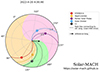 |
Fig. 1. Classification of an SEP event on April 20, 2022, based on the magnetic connections of the space craft considered in this study relative to the flare location. The green, pink, and orange sectors are the sectors of well connected, poorly connected eastern, and poorly connected western events, respectively, with reference to the flare location. The spiral magnetic field lines passing each spacecraft location are indicated by different colours and numbers. L1 (black/number 5) is well connected, and Solar Orbiter (blue/number 4) and Parker Solar Probe (purple/number 3) are poorly connected in the sector of eastern events. BepiColombo (orange/number 2)) and STEREO A (red/number 1) are poorly connected in the sector of western events. The figure is produced with the Solar-MACH tool (Gieseler et al. 2023). |
2.2. Analysis
Our study focuses on the relation between SEP proton and electron peak intensities at various energies and their dependence on the longitudinal separation between the footpoint of the observer’s field line footpoint and the solar source region. In particular, we determine correlations that compare several parameters of the SEP events and their solar sources separately for both well- and poorly connected events. Peak intensities and peak-intensity ratios for protons and electrons as measured by the various spacecraft are compared. We also study the variation of SEP peak intensities with respect to the intensity of the associated soft X-ray flare, and the projected linear speeds of the associated CMEs. The delay in SEP onset with respect to the onset time of the associated flare is also considered. We use the Spearman correlation coefficient (CC, Spearman 1987) to examine the strength of each correlation, and use the p-value to determine the statistical significance of the correlation. A higher p-value indicates a non-significant correlation, while a lower p-value suggests a true, statistically significant correlation. In this work, we consider correlations with p-values of smaller than 0.05 as significant (Spearman 1987). In a few cases, the peak intensity is ‘masked’; for example, there is only a lower limit due to a data gap. The CCs are then calculated both including and excluding the masked points. However, as the correlation coefficients are found to be similar, with very minor differences corresponding to a 1–4 percent error, in the results reported below, all the points with masked peak intensities are included while calculating CCs.
3. Results
Figure 2 shows electron peak intensities as a function of ≥25 MeV proton peak intensities, with ∼100 keV electrons in the top row and 1 MeV electrons in the bottom row. The histograms along the vertical and horizontal axes show the distributions of electron and proton peak intensities, respectively. The left, middle, and right panels in each row show the results for the well-connected events, the poorly connected western events, and the poorly connected eastern events, respectively. The symbols correspond to observations from STEREO A (red triangles), Solar Orbiter (blue circles), L1 (black squares), BepiColombo (orange crosses), and PSP (purple plus signs); points with stars are discussed below. The grey symbols indicate masked points where only a lower limit is provided in the catalogues used. As described in Sect. 2, the peak intensity values are corrected for radial distance effects by scaling to a distance of 1 au. The error bars represent the uncertainties introduced by this radial correction. Spearman correlation coefficients for all the data points (CCall) are provided in the top right corner of each panel. Linear (i.e. power law) relationships between the logarithmic electron and proton intensities are found in several of the plots with medium to high correlations, which are discussed further below. However, an interesting feature in the well-connected sample, especially in the top-left plot, which includes 100 keV electrons, is that some points (highlighted by large stars that follow the same spacecraft colour scheme) seem to lie systematically above the linear trend. These points could be indicative of a different population characterised by higher electron-to-proton ratios. The proton peak intensity histograms at the top of the left-hand plots also suggest the existence of two different proton populations in these well-connected events, splitting at proton peak intensities of around Ip = 10−2 (cm2 sr s MeV)−1.
In the higher Ip population (Ip > 10−2 (cm2 sr s MeV)−1), there is a single linear trend and all electron and proton peak intensities are positively correlated. On the other hand, the lower Ip population (Ip < 10−2 (cm2 sr s MeV)−1) is apparently divided into two subgroups. The events with lower electron intensities appear to follow a similar linear trend to that of the higher Ip population. In addition, as already noted, there is a group of points lying above the rest of the points (marked as large starred points in Fig. 2, left panels); these belong to six independent events. Details of the observations highlighted by large starred points are provided in Table 1. These details include the longitudinal separation angle of the observing spacecraft, ΔΦ, and the peak intensity, Ipeak, corrected for inter-calibration and radial scaling (as described in Sect. 2) for ∼100 keV electrons, 1 MeV electrons, and ≥25 MeV protons. The linear projected speeds and angular widths of the associated CMEs based on LASCO observations are also listed in the Table 1. Observations of these same events by other spacecraft are indicated by small starred points, and interestingly, these observations lie on the linear correlation between electron and proton peak intensities found for the other events. In all, observations of these six events from different spacecraft contribute eight points with large stars and five points with small stars in the plot including 100 keV electrons, and five points with large stars and three points with small stars in the plot including 1 MeV electrons.
Correlation coefficients are provided in the top right corner of each panel. In the case of well-connected events, the CC is provided for all the events, represented as CCall, and for when all the starred events are excluded, represented as CC∼*. We note that all the grey points (where the real peak is masked due to a data gap) lie on the general distribution of data points, except for an outlier in the bottom right corner of the well-connected 1 MeV electron plot (Fig. 2, bottom left), which is excluded from all CC calculations. The values of the correlation coefficients calculated for the sample excluding the starred (both large and small stars) events (CC∼*; points lying along the linear trend; 0.91 for ∼100 keV electrons and of 0.88 for 1 MeV electrons) are much higher, and hence the correlations are more significant, as compared to the values calculated for all the events (CCall; including starred points) for both electron energies (0.76 for ∼100 keV electrons and 0.81 for 1 MeV electrons).
The central and right panels of Fig. 2 show the peak intensities for the groups of poorly connected events in the sectors of western (middle) and eastern (right) events, respectively. In contrast to the group of well-connected events, there is no evidence for the presence of two distinct proton populations in these poorly connected groups and we have therefore calculated only a single correlation coefficient CCall for all the points in each scatter plot. We find that the correlation between electron and proton peak intensities for the eastern events is stronger, and is similar to that for the well-connected events (CC∼*) than for the western events. The different CCs for the eastern events suggest the presence of an asymmetry, with a stronger correlation between electron and proton peak intensities observed when the associated flare is to the east of the observer’s field line footpoint (see also Rodríguez-García et al. 2023a).
Figure 2 also contains information on the presence of DM radio type II bursts, indicating the presence of a shock. The majority of the SEP events in all observer sectors were accompanied by a DM type II radio burst; the encircled points indicate the exceptions, where no DM type II burst was observed (see also Table A.1).
Figure 3 shows the ratio of electron to proton peak intensities (e/p) as a function of proton peak intensities for the well-connected (left) and poorly connected western (middle) and eastern (right) events. The symbols are the same as in Fig. 2 and again the clear outlier, the grey point with a low masked peak intensity, is excluded from the calculation of the CCs for the well-connected events. The scatter plots for the well-connected group, especially for 100 keV electrons (top), clearly show the group of six events with high e/p values indicated by the large starred points inside the grey circle in the 100 keV electron plot.
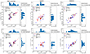 |
Fig. 2. Peak intensities of ∼100 keV electrons (top panels), and 1 MeV electrons (bottom panels) as a function of ≥25 MeV proton peak intensities for well-connected events (left), western events (middle), and eastern events (right). Red triangles, blue circles, black squares, orange crosses, and purple plus symbols indicate the STEREO A, Solar Orbiter, L1, BepiColombo, and PSP observations, respectively. Large starred points following the same colour scheme highlight events that deviate from the linear trend. Small starred points represent the measurements of the same events by other spacecraft that are more consistent with the linear trend. Encircled points indicate events where no DM type II radio burst was reported. Error bars represent the error in heliocentric radial scaling measurements. CCs are provided in the legend boxes with the first value denoting the correlation coefficient, and the second (in parentheses) giving the p-value. For the well-connected events, two CCs are provided: CCall for all the events in the scatter plot, and CC∼* for the rest of the events, excluding the starred (both large and small) points. The histograms along the vertical axes show the distribution of electron peak intensities, and those along the horizontal axes show the distribution of proton peak intensities. |
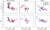 |
Fig. 3. Electron-to-proton peak intensity ratios for ∼100 keV electrons (top panels), and 1 MeV electrons (bottom panels) as a function of peak intensities of ≥25 MeV protons for well-connected (left), western (middle), and eastern (right) events. All symbols are the same as in Fig. 2. Large starred points highlight the group of events with high e/p ratios that lie above the linear trend in Figure 2, while the small starred points that lie on the linear trend represent the observations from same events (large starred points) taken at some other spacecraft. |
Figure 4 compares the peak intensities of ∼100 keV electrons (I100keV) with those of 1 MeV electrons (I1MeV) for well-connected (left) and poorly connected western (middle) and eastern (right) events, again using the same symbols. The strongest correlation, excluding the outlier points, is found for the well-connected events, as shown by CCall = 0.90 and CC∼* = 0.92 when the starred events are included or excluded, respectively. The poorly connected western and eastern events also show strong correlations, each having CCall = 0.86. There is no clear indication of two different populations at either electron energy, and all the points align along one quasi-linear trend.
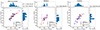 |
Fig. 4. Peak intensities of ∼100 keV electrons as a function of peak intensities of 1 MeV electrons for well-connected (left), western (middle), and eastern (right) events. All symbols are the same as in Fig. 2. CCall and CC∼* are the Spearman correlation coefficient along with the p-value, for all the events in scatter plot, and for the rest of the events, excluding the starred points, respectively, for well-connected events (left) and for poorly connected events (middle and right). |
Figure 5 shows the distribution of the ratio of I100keV to I1MeV peak intensities for well-connected (top) and poorly connected western (centre) and eastern (bottom) events. This ratio can be interpreted in terms of a spectral index, with higher ratios corresponding to steeper spectra and lower ratios to flatter spectra. The distributions do not show any clear differences, suggesting that the spectra are similar for each sample of events, though the statistics are limited.
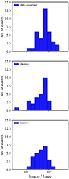 |
Fig. 5. Histograms showing the distribution of the ratio of ∼100 keV to 1 MeV electron peak intensities for well-connected (top), western (centre), and eastern (bottom) events. |
As a comparison with the results using the limited number of SERPENTINE events, Fig. 6 shows histograms of ∼25 MeV proton peak intensities from an updated version (Richardson 2024) of the SEP event catalogue of Richardson et al. (2014). This catalogue includes measurements made by STEREO A, STEREO B, and SOHO from December 2006 to January 2023. The SEP events are grouped into well-connected (top) and poorly connected (bottom) events using the criteria introduced in Sect. 2.1. As noted above, there is a clear suggestion of two populations in the small sample of well-connected events shown in the proton histograms in Fig. 2 (left), and the histogram for the well-connected events in the top panel of Fig. 6 also suggests the presence of two distributions, split at Ip ∼ 10−1 (cm2 sr s MeV)−1. We performed a Gaussian mixture modelling (GMM; see Appendix C) statistical test to investigate whether there are multiple distinct SERPENTINE and Richardson (2024) events. This test demonstrates that both data sets show similar mean values when assuming two distinct distributions, suggesting that the data sets are similar. Furthermore, the test suggests that the sample of Richardson et al. (2014) is composed of two or three distinct groups, whereas our sample is best explained by two groups. We note that, in Fig. 12 of Richardson et al. (2014), the well-connected events include both a large population of small events that were only observed at one or two spacecraft locations and large SEP events that were observed at all locations; such a distinction is less evident in Fig. 6. The histogram for the poorly connected events in Fig. 6 (bottom) clearly shows no evidence of two populations, suggesting that the poorly connected events that include the flanks of large SEP events are more homogeneous.
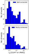 |
Fig. 6. Histograms of peak intensities of ∼25-MeV proton events based on an extended version (Richardson 2024) of the SEP event catalogue of Richardson et al. (2014) for well-connected (top), and poorly connected (bottom) events during December 2006 – January 2023. |
In Fig. 7, the dependence of SEP intensities on the intensity of the associated flare is studied for ∼100 keV electrons (top), 1 MeV electrons (centre), and ≥25 MeV protons (bottom) in well-connected (left) and poorly connected western (middle) and eastern (right) events; symbols are the same as in previous similar figures. An associated flare is identified for 40 of the 45 SEP events in this sample. As described above in Sect. 2, 32 of these associations are based on observations from the Earth-orbiting GOES spacecraft, while in eight cases, the flares were behind the limb as seen from Earth and observed by Solar Orbiter/STIX, where the estimated GOES class is based on the counts in the STIX 4–10 keV channel, using a statistical correlation between the GOES 1–8 Å flux and the STIX 4–10 keV channel. The measurement uncertainty is represented by error bars parallel to the x-axis.
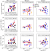 |
Fig. 7. Peak intensities of SEPs as a function of flare intensity for ∼100 keV electrons (top panel), 1 MeV electrons (central panel) and ≥25 MeV protons (bottom panel) for well-connected (left), western (middle), and eastern (right) events. All symbols are same as in Fig. 2. CCall and CC∼* are the Spearman correlation coefficients along with p-value, for all the events in the scatter plot, and for the rest of events, excluding the starred points, respectively. CC* is the Spearman correlation coefficient along with p-value considering only the starred points in the well-connected events. Error bars along the x-axis represent the uncertainty in the estimated GOES-equivalent flare intensity in case of behind the limb flares observed by Solar Orbiter/STIX. |
We note that a single flare in Fig. 7 may be associated with several SEP observations that may fall into different longitudinal sectors (well-connected and poorly connected western and eastern). For the well-connected events (Fig. 7, left), an additional correlation coefficient (CC*) is calculated for the group of six events indicated by starred points, including both the large starred points in high e/p ratios that deviate from the linear trend in Fig. 3 and the small starred points with low e/p ratios that are consistent with the linear trend in Fig. 3. We find high CC* values for the starred events between the flare strength and electron intensities. However, due to the small number of data points (eight points), the CC* for 1 MeV electrons is not reliable. For protons, we find a smaller correlation with the flare strength when only considering all the large and small starred points.
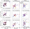 |
Fig. 9. Peak intensities of SEPs as a function of projected linear CME speed for ∼100 keV electrons (top panel), 1 MeV electrons (central panel), and ≥25 MeV protons (bottom panel) for well-connected (left), western (middle), and eastern (right) events. All symbols are the same as in Fig. 2. CCall and CC∼* are the Spearman correlation coefficients along with the p-values for all events in the scatter plot, and for the rest of events, excluding the starred points, respectively. |
No further significant correlations are observed for protons in any of the three sectors, or for either of the two electron energies in any of the poorly connected sectors. The CCs for 1 MeV electrons (centre) and > 25 MeV protons (bottom) are slightly higher for poorly connected eastern events than those for western events, suggesting an east–west asymmetry in the dependence on the intensity of the associated flare.
Figure 8 reproduces the left-hand row (well-connected events) of Fig. 7 but highlights the star-symbol data points –which show stronger correlations with the flare strength– by plotting the other points with lighter colours. Because the events indicated by large starred points, which are characterised by enhanced electron-to-proton ratios, are only found in the well-connected sector (cf., Figs. 2 and 3), we furthermore suggest that these could be candidates for flare-dominated events, where electrons are accelerated more efficiently than protons. Indeed, while the proton peak intensities do not show any dependence on the flare strength, the electrons, especially the 100 keV electrons, show medium strength correlations. (As noted above, error bars parallel to the x-axis indicate uncertainties in the intensity of behind-the-limb flares inferred from STIX observations.)
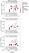 |
Fig. 8. Peak intensities of SEPs as a function of flare intensity for ∼100 keV electrons (top panel), 1 MeV electrons (central panel), and ≥25 MeV protons (bottom panel) for well-connected events. All symbols are the same as in Fig. 7. Large starred points represent some of the observations from a group of six SEP events, standing out from the linear trend, and small starred points represent the observations from the same six events with measurements taken at some other spacecraft, and fit into the linear trend. All the rest of points are represented in lighter colours to highlight the starred points only. CCall and CC∼* are the Spearman correlation coefficients along with the p-value for all the events in the scatter plot, and for the rest of the events, excluding all the starred points, respectively. CC* is the Spearman correlation coefficient along with the p-value considering only the starred (both large and small) points in the well-connected events. Error bars along the x-axis represent the uncertainty in the estimated GOES-equivalent flare intensity in the case of behind-the-limb flares observed by Solar Orbiter/STIX. |
Furthermore, in Appendix C, our event sample is tested for clusters using the three parameters, proton peak intensity Ip, flare intensity Iflare, and ratio of the 100 keV electron to ≥25 MeV proton peak intensities I100 keV/Ip. The clustering analysis suggests that all except two of the starred events –which were classified as outliers– belong to a distinct SEP event group out of three groups in total.
In Fig. 9, the relationship between SEP peak intensities and the projected linear speeds of the associated CMEs (enlisted in Table A.1) is studied. The figure is organised is a similar way to Fig. 7. Again, the masked outlier point highlighted in grey in the left, middle, and bottom panels is excluded from the calculation of all CCs.
None of the scatter plots in Fig. 9 show a strong correlation. It is only for the 100 keV electrons in the well-connected sector that we find a medium strong correlation of (0.48).
In Fig. 10, the relationship between X-ray flare intensities and the projected linear speeds of associated CMEs is studied for the whole sample. Details of these parameters are provided in Table A.1. The encircled points represent events where no DM radio type II burst is reported. Once again, error bars parallel to the x-axis indicate uncertainties in the behind-the-limb flare intensities from STIX.
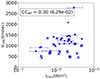 |
Fig. 10. Variation of the projected linear CME speed as compared to the flare intensity. Large starred points represent the group of events with high e/p ratios that deviate from the linear trend in blue Fig. 2, and small starred points represent the same events observed at other locations that lie on the linear trend in Fig. 2. Encircled points represent events where no DM radio type II burst is reported. Error bars along the x-axis represent the uncertainty in the estimated GOES-equivalent flare intensity in the case of behind-the-limb flares observed by Solar Orbiter/STIX. CCall displays the correlation coefficient of all the points marked by symbols (not taking into account the error bars). |
Surprisingly, there is only a weak correlation (CCall = 0.30) between the flare intensity and CME speed. This value is lower than values found in previous studies, such as the 0.61 ± 0.11 noted by Rodríguez-García et al. (2023a) for example.
Fig. 11 shows the peak intensities of ∼100 keV (red symbols) and 1 MeV electrons (blue symbols) as a function of the longitudinal separation angle ΔΦ between the flare and the observer’s field line footpoint. The vertical green dashed lines and green arrow indicate the range of the well-connected events, and similarly, the orange and pink arrows mark the sectors of poorly connected western and eastern events, respectively. The top panel includes all events observed at either of the two electron energies. The central panel shows those events simultaneously observed at both electron energies, while those events only observed at one of the two energies are displayed in the bottom panels; these latter are mostly observed only at ∼100 keV (red symbols) rather than only at 1 MeV (blue symbols), as they are most likely weak events that do not extend to higher energies. The few events where a corresponding ∼100 keV electron intensity is missing (blue points in the bottom panel) are either caused by data gaps or ion contamination during the peak phase of the event. While the highest peak intensities in the whole sample tend to be associated with events observed within or close to the well-connected sector, an overall dependence of electron peak intensities on the longitudinal separation angle is not observed. Rather, the intensities show a large scatter, including events with small peak intensities observed in the well-connected sector and events with high peak intensities that are observed at large longitudinal separations. Thus, the longitudinal dependence of the peak intensities is likely to be related not only to the longitudinal separation but also to the nature and strength of the solar source and the intrinsic intensity of the particle event.
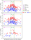 |
Fig. 11. Electron peak intensities for both electron energies, that is, ∼100 keV (red symbols) and 1 MeV electrons (blue symbols), as a function of the longitudinal separation angle ΔΦ. The green, orange, and pink arrows indicate the sectors of well-connected, western, and eastern events, respectively. The top panel includes all events observed at any of the two electron energies. The central panel shows those events simultaneously observed at both electron energies, while those events only observed at one of the two energies (∼100 keV and 1 MeV) are displayed in the bottom panel. |
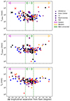 |
Fig. 12. Variation of the onset delay time of SEP events from flare onset with respect to the longitudinal separation ΔΦ of the observer’s field line footpoint from the flare location for 1 MeV electrons (top panel), ∼100 keV electrons (central panel), and ≥25 MeV protons (bottom panel). All symbols are the same as in Fig. 2. Green, orange, and pink arrows represent the sectors of well-connected and poorly connected western and eastern events, respectively. |
In Fig. 12 we study the delay between the flare start and the onset of the associated SEP event at the observing spacecraft, and its relation with the longitudinal separation angle for 1 MeV electrons (top), ∼100 keV electrons (middle), and ≥25 MeV protons (bottom). The symbols are the same as in Fig. 2. The different longitudinal sectors are represented as they are in Fig. 11. The largest proton and electron onset delays are found in the western and eastern events. Interestingly, there is a large range of onset delays for all particle species, even in the well-connected events, where small onset delays might be expected.
4. Discussion
In this work, we investigated electron and proton peak intensities and their ratios in large SEP events to study the contribution of flares and shocks as potential sources of particle acceleration in large SEP events. We used a sample of 45 SEP events from November 2020 to May 2023 from the SERPENTINE catalogue (Dresing et al. 2024a,b), which provides measurements made by multiple spacecraft (i.e. Solar Orbiter, STEREO A, the near-Earth spacecraft (SOHO, Wind), BepiColombo, and PSP). We used electrons of two energies (∼100 keV and 1 MeV) and ≥25 MeV protons, and categorised the events depending on their longitudinal sector based on the separation between the observing spacecraft’s field line footpoint and the location of the associated flare. We also investigated the correlations between the particle peak intensities and the soft X-ray flare intensity and the associated projected linear CME speeds.
Although we examined a comparatively small sample of 45 multi-spacecraft SEP events, these provided over 140 individual event observations spanning a time interval of 31 months. Our results are consistent with those of Cliver & Ling (2007), who found evidence for two distinct SEP populations in well-connected SEP events, which are assumed to represent a flare- and a shock-related population (see Sect. 1).
Similarly, two populations are evident in the histogram of proton peak intensities for well-connected events (as shown in Fig. 2, left, top panels), splitting at Ip ∼ 10−2 (cm2 sr s MeV)−1. To confirm the presence of two distinct populations in the proton intensities for well-connected events, we applied the statistical test described in Appendix C to the data set used for this study and also to a sample of observations from an extended Solar Cycle 24 event list updated from Richardson et al. (2014). Results of the statistical test indicate that the well-connected events in both data sets consist of two subpopulations, one with lower and one with higher proton peak intensities.
The presence of two distinct populations is further supported by the scatter plots of electron versus proton peak intensities in the well-connected sector in Fig. 2 (left, panels). These plots show an overall good correlation between the electron and proton peak intensities, but also a separate group of events with low proton intensities and high e/p ratios, which lie outside the general correlation trend (these events are marked by large starred points in all plots and details of these large starred observations are provided in Table 1). Similar populations of weak proton events with high e/p-ratios are not found in the poorly connected samples. These results suggest that the weak, high-e/p-ratio, well-connected events are most likely dominated by flare-accelerated particles.
In a similar analysis, Cane et al. (2010) supported the idea of a single event population instead of two distinct populations. Their conclusions were based on a continuous distribution of electron to proton ratios, which did not show any distinct populations of relatively electron-rich and electron-poor events. In our well-connected group of events, we cannot confirm such a continuum of e/p-ratios. When plotting the e/p ratios as a function of proton peak intensities (Fig. 3), we again see the additional population standing out of the linear trend of the rest of the scatter plot, suggesting that a stronger flare contribution is present in the low-Ip regime. A cluster analysis (shown in Appendix C) taking into account the proton peak intensity, the electron to proton ratio, and the flare intensity further supports that these high-e/p-ratio events form a distinct subgroup out of the three distinct groups suggested by the clustering analysis.
Both the poorly connected western and eastern groups show strong correlations between electron and proton peak intensities, and we find no evidence for the presence of two separate populations. Because of the larger extent of the CME-driven shock compared to the flare, which allows it to also connect to poorly connected observers, we conclude that for poorly connected events, the source is mainly shock-related, which is again in agreement with the results of Cliver & Ling (2007). When comparing the western and eastern events, we observe much higher CCs for eastern events for both electron energies, suggesting a longitudinal asymmetry. This could mean that shocks accelerate the SEPs more efficiently in the eastern sector compared to the western sector. Similar results on eastern asymmetry are reported by Rodríguez-García et al. (2023a).
Table 2 summarises the Spearman CCs calculated for all the correlations determined in this study. The first value denotes the CC, while the second one in parentheses provides the p-value. The number of data points included in the calculation of each CC included in the table is listed below the corresponding CC value. For the well-connected events, we provide the coefficients CCall, which is for all the points in the scatter plot, and CC∼*, which is for all points excluding all the starred points (large with high e/p ratios and small with low e/p ratios). Some correlations were found to be small or insignificant, which is partly caused by the small statistics of our event sample. We therefore highlight those entries that have |CC|> 0.5 and a statistical significance of at least 5% (p-value < 0.05) in bold in Table 2.
Spearman correlation coefficients (p-values) for different correlations studied.
The high correlation between the electron and proton peak intensities in poorly connected regions (as well as in the well-connected region when excluding the high-e/p-ratio events (CC∼*) suggests that both species are not only accelerated by the shock but also accelerated in a similarly efficient way.
A clear discrepancy between our results and those of Cliver & Ling (2007) is related to the presence or absence of type II radio bursts. The majority of our events are accompanied by a DM type II radio burst (as observed by spacecraft-based instrumentation), marking the presence of a shock. Those events missing a DM type II burst are marked by encircled symbols in our scatter plots. Contrary to Cliver & Ling (2007), we find the presence and absence of type II bursts to be similar in the well-connected and poorly connected samples, while Cliver & Ling (2007) found radio bursts to be mostly absent in their flare-associated group. Even when considering only our high-e/p-ratio events, we find only three out of the eight events to be lacking a DM type II burst.
Focusing on the electron peak intensities, we find a strong and significant correlation between the ∼100 keV and 1 MeV electrons in all sectors. These are among the highest correlations of our analysis, and are mostly stronger than the correlations with proton peak intensities. This suggests a similar origin for 100 keV and 1 MeV electrons in our sample. The histogram of electron peak intensity ratios (Fig. 5) provides a rough measure of electron energy spectra, with larger ratios denoting softer spectra and smaller ratios harder spectra. In contrast to results by Cliver & Ling (2007), we do not find any evidence for the presence of two distinct populations when comparing the two electron energy ranges. Among the eight high-e/p-ratio points, five are still seen in 1 MeV electrons.
Comparing the SEP peak intensities with the soft-X-ray intensities of the associated flares reveals significantly smaller correlations than those discussed above. The small correlations in the well-connected sample are particularly surprising, as a flare contribution is expected in this region. The significantly weaker correlation (for the whole sample) for protons (CCall = 0.36 compared to CCall ∼ 0.5, for electrons) could be caused by the relatively small sample size of events, which show large flare intensities but small proton intensities. Interestingly, these are mostly the same points (large starred) that show high e/p ratios, which we earlier associated to flare-dominated events. Excluding these presumably flare-dominated events from the correlation with the flare intensity leads to an increased correlation coefficient (CC∼* = 0.46 with p-value = 5.71 10−3) for protons. The overall small correlations with the flare strength suggest that the role of the flare was overall minor in producing the energetic SEP events of our sample. The correlation coefficients for the group of presumably flare-dominated events are also calculated separately as CC* = 0.68 and 0.26 for ∼100 keV electrons and ≥25 MeV protons, respectively, supporting the assumption that the star-symbol events mark those few events of our sample where the flare provided the dominant source.
The absence of any clear correlation between SEP peak intensities and CME linear speeds might be surprising given the hypothesis that the CME-driven shock plays the main role in most events. However, as we are using only values based on SOHO/LASCO observations, the CME linear speeds likely suffer from projection effects.
All of the members of the group of six presumably flare-dominated events are accompanied by a CME (Table A.1). Furthermore, we do not find that these CMEs are slower or narrower compared to the whole sample. As can be seen in Table 1, the CMEs associated with the presumably flare-dominated events show a variation of projected linear speeds and angular widths, including fast and halo CMEs.
Previous multi-spacecraft SEP studies have reported a peak-intensity dependence on the longitudinal separation angle (e.g. Lario et al. 2006, 2013; Dresing et al. 2014; Richardson et al. 2014). Figure 11 shows that, in our sample, the largest peak intensities are observed in the well-connected sector and that intensities generally also decrease with increasing separation angle. However, we observe a strong event-to-event variation, including cases with large peak intensities at poorly connected observer locations. This suggests that these poorly connected events are not predominantly caused by transport effects (e.g. Dresing et al. 2012; Dröge et al. 2010; Strauss et al. 2017), such as perpendicular diffusion, which would cause depleted intensities, but that these events are rather produced by a direct connection to a shock potentially accelerating the SEPs more efficiently in the sector of eastern events. Similarly, a larger event-to-event variation is observed for the longitudinal dependence of onset delays (Fig. 12). Longer onset delays are especially expected in cases of significant perpendicular diffusion (e.g. Strauss et al. 2017; Dresing et al. 2014). Our sample shows such significantly longer onset delays mostly in the sector of far western events for electrons and in the sector of far eastern events for protons, potentially pointing towards an asymmetry. However, due to the low number of points at poorly connected regions, this asymmetry is hard to corroborate.
Our work does not reveal significant differences between 100 keV and 1 MeV electrons, which were suggested to be dominated by flares and shocks, respectively (Dresing et al. 2022). However, it is likely that most of the events in our sample are shock dominated. This is due to the selection criterion for the SEP catalogue we used, which was based on the presence of a multi-spacecraft 25–40 MeV proton event. This makes the presence of a shock very likely, especially when the different spacecraft observing the proton event are significantly separated from each other, meaning that at least one of them is likely a poorly connected observer.
5. Conclusions
In summary, we find evidence for the presence of two distinct SEP sources, which –based on the interpretation of Cliver & Ling (2007)– are most-likely the flare and the CME-driven shock. We find that the relation of electron and proton peak intensities is a useful tool for identifying flare-dominated events, or at least those events where a shock contribution is missing. Using this tool we find that about 6 single-spacecraft observations out of the 45 multi-spacecraft events show significantly higher electron-to-proton ratios than those found in the rest of the sample. These are most likely flare dominated, showing us that the flare accelerates both electrons and protons but with different efficiencies. On the contrary, the high correlations found between electron and proton peak intensities, especially in the poorly connected sectors, suggest that the shock not only accelerates both species but that it does so with very similar efficiency. We note that the subsample of well-connected events that show low proton peak intensities in the well-connected sector are the most challenging to be characterised and likely constitute a mixture of flare and shock acceleration.
Data availability
A comprehensive table containing all parameters employed in this study for the analysed SEP event sample is provided on Zenodo at https://zenodo.org/records/14161713. The SERPENTINE SEP event catalogue is available at https://data.serpentine-h2020.eu/catalogs/sep-sc25/ and at https://zenodo.org/doi/10.5281/zenodo.10732268. For our study, we used the updated version 3 of the list, in which information on several associated flares was updated.
The SERPENTINE multi-spacecraft SEP event catalogue contains information on radio type II bursts using both spacecraft and ground-based observations.
The SERPENTINE-CME list is available at https://data.serpentine-h2020.eu/catalogs/cme/
Acknowledgments
We thank the anonymous reviewers for their careful and constructive referee report. We acknowledge funding by the European Union’s Horizon 2020/Horizon Europe research and innovation program under grant agreement No. 101004159 (SERPENTINE) and No. 101134999 (SOLER). G.U.F. acknowledges funding by Finnish National Agency for Education (EDUFI grant No. OPH-4056-2021). N.D. and L.V. are grateful for support by the Academy of Finland (SHOCKSEE, grant No. 346902). L.V. acknowledges the financial support of the University of Turku Graduate School. I.G.R. acknowledges support from NASA programs NNH19ZDA001N-HSR and NNH19ZDA001N-LWS and travel support from the SERPENTINE project. L.R.-G. acknowledges support through the European Space Agency (ESA) research fellowship programme.
References
- Benkhoff, J., Murakami, G., Baumjohann, W., et al. 2021, Space Sci. Rev., 217, 90 [NASA ADS] [CrossRef] [Google Scholar]
- Campello, R. J. G. B., Moulavi, D., & Sander, J. 2013, in Advances in Knowledge Discovery and Data Mining, eds. J. Pei, V. S. Tseng, L. Cao, H. Motoda, & G. Xu (Berlin, Heidelberg: Springer, Berlin Heidelberg), 160 [Google Scholar]
- Campello, R. J. G. B., Moulavi, D., Zimek, A., & Sander, J. 2015, ACM Trans. Knowl. Discov. Data, 10, 1 [CrossRef] [Google Scholar]
- Cane, H. V., von Rosenvinge, T. T., Cohen, C. M. S., & Mewaldt, R. A. 2003, Geophys. Res. Lett., 30, 8017 [NASA ADS] [Google Scholar]
- Cane, H. V., Mewaldt, R. A., Cohen, C. M. S., & von Rosenvinge, T. T. 2006, J. Geophys. Res. (Space Phys.), 111, A06S90 [NASA ADS] [CrossRef] [Google Scholar]
- Cane, H. V., Richardson, I. G., & von Rosenvinge, T. T. 2010, J. Geophys. Res. (Space Phys.), 115, A08101 [Google Scholar]
- Cliver, E. W., & Ling, A. G. 2007, ApJ, 658, 1349 [NASA ADS] [CrossRef] [Google Scholar]
- Domingo, V., Fleck, B., & Poland, A. I. 1995, Sol. Phys., 162, 1 [Google Scholar]
- Dresing, N., Gómez-Herrero, R., Klassen, A., et al. 2012, Sol. Phys., 281, 281 [NASA ADS] [Google Scholar]
- Dresing, N., Gómez-Herrero, R., Heber, B., et al. 2014, A&A, 567, A27 [NASA ADS] [CrossRef] [EDP Sciences] [Google Scholar]
- Dresing, N., Kouloumvakos, A., Vainio, R., & Rouillard, A. 2022, ApJ, 925, L21 [NASA ADS] [CrossRef] [Google Scholar]
- Dresing, N., Yli-Laurila, A., Valkila, S., et al. 2024a, A&A, 687, A72 [NASA ADS] [CrossRef] [EDP Sciences] [Google Scholar]
- Dresing, N., Yli-Laurila, A., Valkila, S., et al. 2024b, https://doi.org/10.5281/zenodo.13710527 [Google Scholar]
- Dröge, W., Kartavykh, Y. Y., Klecker, B., & Kovaltsov, G. A. 2010, ApJ, 709, 912 [CrossRef] [Google Scholar]
- Fox, N. J., Velli, M. C., Bale, S. D., et al. 2016, Space Sci. Rev., 204, 7 [Google Scholar]
- Gieseler, J., Dresing, N., Palmroos, C., et al. 2023, Front. Astron. Space Sci., 9, 384 [NASA ADS] [CrossRef] [Google Scholar]
- Huovelin, J., Vainio, R., Kilpua, E., et al. 2020, Space Sci. Rev., 216 [CrossRef] [Google Scholar]
- Kaiser, M. L., Kucera, T. A., Davila, J. M., et al. 2008, Space Sci. Rev., 136, 5 [Google Scholar]
- Lario, D., Kallenrode, M.-B., Decker, R. B., et al. 2006, ApJ, 653, 1531 [NASA ADS] [CrossRef] [Google Scholar]
- Lario, D., Aran, A., Gómez-Herrero, R., et al. 2013, ApJ, 767, 41 [CrossRef] [Google Scholar]
- Lin, R. P., Anderson, K. A., Ashford, S., et al. 1995, Space Sci. Rev., 71, 125 [CrossRef] [Google Scholar]
- McComas, D. J., Alexander, N., Angold, N., et al. 2016, Space Sci. Rev., 204, 187 [Google Scholar]
- McInnes, L., Healy, J., & Astels, S. 2017, J. Open Source Software, 2, 205 [NASA ADS] [CrossRef] [Google Scholar]
- McKibben, R. B. 1972, J. Geophys. Res. (1896-1977), 77, 3957 [CrossRef] [Google Scholar]
- Moulavi, D., Jaskowiak, P. A., Campello, R. J. G. B., Zimek, A., & Sander, J. 2014, in SDM, eds. M. J. Zaki, Z. Obradovic, P. N. Tan, et al. (SIAM), 839 [Google Scholar]
- Müller, D., St. Cyr, O. C., Zouganelis, I., et al. 2020, A&A, 642, A1 [Google Scholar]
- Müller-Mellin, R., Kunow, H., Fleissner, V., et al. 1995, Sol. Phys., 162, 483 [CrossRef] [Google Scholar]
- Müller-Mellin, R., Böttcher, S., Falenski, J., et al. 2008, Space Sci. Rev., 136, 363 [Google Scholar]
- Ogilvie, K. W., & Desch, M. D. 1997, Adv. Space Res., 20, 559 [Google Scholar]
- Reames, D. V. 2013, Space Sci. Rev., 175, 53 [CrossRef] [Google Scholar]
- Reynolds, D. 2009, in Gaussian Mixture Models, eds. S. Z. Li, & A. Jain (Boston, MA: Springer, US), 659 [Google Scholar]
- Richardson, I. 2024, Solar Energetic Particle Events Including ∼ 25 MeV Protons Observed at STEREO and/or Earth since 2006, https://doi.org/10.7910/DVN/GQPCXZ, Harvard Dataverse, V3 [Google Scholar]
- Richardson, I. G., von Rosenvinge, T. T., Cane, H. V., et al. 2014, Sol. Phys., 289, 3059 [NASA ADS] [CrossRef] [Google Scholar]
- Rodríguez-García, L., Balmaceda, L. A., Gómez-Herrero, R., et al. 2023a, A&A, 674, A145 [NASA ADS] [CrossRef] [EDP Sciences] [Google Scholar]
- Rodríguez-García, L., Gómez-Herrero, R., Dresing, N., et al. 2023b, A&A, 670, A51 [NASA ADS] [CrossRef] [EDP Sciences] [Google Scholar]
- Rodríguez-Pacheco, J., Wimmer-Schweingruber, R. F., Mason, G. M., et al. 2020, A&A, 642, A7 [Google Scholar]
- Roelof, E. C., Gold, R. E., Simnett, G. M., et al. 1992, Geophys. Res. Lett., 19, 1243 [NASA ADS] [CrossRef] [Google Scholar]
- Spearman, C. 1987, Am J. Psychol., 100, 441 [Google Scholar]
- Stoica, P., & Selen, Y. 2004, IEEE Signal Process. Mag., 21, 36 [CrossRef] [Google Scholar]
- Strauss, R. D. T., Dresing, N., & Engelbrecht, N. E. 2017, ApJ, 837, 43 [NASA ADS] [CrossRef] [Google Scholar]
- Torsti, J., Valtonen, E., Lumme, M., et al. 1995, Sol. Phys., 162, 505 [CrossRef] [Google Scholar]
- Trottet, G., Samwel, S., Klein, K. L., Dudok de Wit, T., & Miteva, R. 2015, Sol. Phys., 290, 819 [Google Scholar]
- von Rosenvinge, T. T., Reames, D. V., Baker, R., et al. 2008, Space Sci. Rev., 136, 391 [Google Scholar]
- Wilson, Lynn B. I., Brosius, A. L., Gopalswamy, N., et al. 2021, Rev. Geophys., 59, e2020RG000714 [NASA ADS] [CrossRef] [Google Scholar]
- Xiao, H., Maloney, S., Krucker, S., et al. 2023, A&A, 673, A142 [NASA ADS] [CrossRef] [EDP Sciences] [Google Scholar]
Appendix A: Additional table
Table A.1 summarises details of the associated flares, CMEs, and Type II radio bursts (both metric and DM) reported for the analysed SEP events. The coordinates of the flare location are provided in Carrington coordinates. Projected linear speeds of only the most likely CME candidates to be associated with the respective SEP event based on SOHO/LASCO observations are enlisted.
Flares, CMEs, and Type II radio bursts associated with the analysed SEP events.
Appendix B: Electron inter-calibration
As noted by Lario et al. (2013) and Richardson et al. (2014), the intensities of ∼1 MeV electrons measured by STEREO A/HET were lower by a factor of ∼15 than those measured by instruments on SOHO during the SEP events in December 2006, when the STEREO spacecraft were still close to Earth. Here, we use the decay phases of several SEP events to investigate the inter-calibration of STEREO A/HET and Solar Orbiter/HET. The decay phases of SEP events are well-suited for inter-calibration because the particle distributions are usually near-isotropic so that the measured particle intensities are independent of the telescope viewing direction or the direction of the magnetic field. In addition, SEP intensities during the decay phase tend to be less dependent on longitude (the “reservoir effect" e.g., McKibben 1972; Roelof et al. 1992). We considered the decay phases of four SEP events (2021-10-09, 2021-10-28, 2022-01-20, and 2023-02-25) simultaneously observed by both instruments, and the variations of intensity profiles of 1 MeV and ∼100 keV electrons (from STEREO SEPT and SolO EPT) were studied. We assume that, due to the similarity of SEPT and EPT, the ∼100 keV electron intensities measured by these instruments are already on a common baseline. Then, assuming that the shape of the electron spectrum and its evolution during the decay phases of the events is similar at both spacecraft, then any difference between the 1 MeV electron intensities measured by the STEREO and SolO HETs at the same ∼100 keV intensity level indicates a difference in the response of these two instruments.
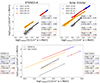 |
Fig. B.1. Peak intensities of 1 MeV electrons versus peak intensities of ∼100 keV electrons measured at STEREO A/SEPT & HET (top-left) and Solar Orbiter/EPT & HET (top-right) for four commonly observed events at both spacecraft. Legend boxes with corresponding colours have the values of slope and y-intercept for each fit on the scatter plots. The lower panel shows fits for the events observed by both spacecraft, with solid and dotted lines representing Solar Orbiter and STEREO A observations, respectively. |
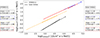 |
Fig. B.2. The alignment of STEREO A and Solar Orbiter fits achieved by adding 1 (= a factor of 10) to the logarithmic STEREO A intercepts. Solid and dotted lines represent Solar Orbiter and STEREO A observations, respectively. Legend boxes with corresponding colours give the slope and y-intercept for each fit. |
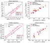 |
Fig. B.3. Re-normalization applied to PSP measurements for 1 MeV (top panel) and ∼100 keV (lower panel) electrons. The left panel shows the fits applied to STEREO A and PSP data points, for 1 MeV (top panel) and ∼100 keV (lower panel) electrons. The right panel shows the results of PSP re-normalization applied to 1 MeV (top panel) and ∼100 keV (lower panel) electrons. In the right panel, orange and purple plus markers represent the PSP data points before and after the re-normalization, respectively. |
Figure B.1 (top panel) shows the scatter plots of intensities of 1 MeV electrons against the intensities of ∼100 keV electrons measured by STEREO A (top-left) and Solar Orbiter (top-right) for same decay phase intervals, with each event shown by different colour points. Each scatter plot is fitted with a straight line, and slope and y-intercept are shown in the legend box with the corresponding colour. Figure B.1 (lower panel) shows only the fits to both spacecraft measurements, where solid and dotted lines indicate Solar Orbiter and STEREO A measurements, respectively. To infer the inter-calibration factor for the HETs, the y-intercepts of all of STEREO A data fits are raised by different factors to so that they align with those for SolO. By comparing the individual values, the best possible common line up is then determined by raising all fits to STEREO A/HET data values (dotted lines) by an addition of 1 on the log-scale axis (Fig. B.2) resulting in an inter-calibration factor of 101 = 10 for STEREO A/HET measurements. Thus, STEREO A/HET measurements are multiplied by a factor of 10 for all SEP events in the analysis.
Figure B.3, left column, shows the 1 MeV (top) and 100 keV (bottom) electron peak intensities as a function of 25-MeV proton peak intensities as observed by STEREO A (after re-calibration) and PSP, corrected for the distance of the spacecraft as described in Sect. 2. While the dependence of the electron vs. proton intensity is similar in both sets of observations, it appears that PSP observations of 1 MeV (100 keV) electrons are systematically higher (lower) than re-calibrated STEREO A observations for a given 25-MeV proton peak intensity. We, therefore, apply a constant factor to PSP data to bring it to the same baseline as STEREO A (and Solar Orbiter). The best-fit multiplier for PSP is obtained by determining which factor CPSP brings the PSP points into best agreement with the model obtained by fitting electron peak intensities against proton peak intensities for STEREO A (the red best-fit lines in the left column of Fig. B.3). Thus, we find the value of CPSP minimizing
![Mathematical equation: $$ \begin{aligned} \chi ^2 = \sum _{i = 1}^{N^\mathrm{PSP}} [\log I_{\mathrm{e},i}^\mathrm{PSP}+\log C^\mathrm{PSP} - (a^\mathrm{STA}+b^\mathrm{STA}\log I_{\mathrm{p},i}^\mathrm{PSP})]^2, \end{aligned} $$](/articles/aa/full_html/2025/01/aa50945-24/aa50945-24-eq1.gif) (B.1)
(B.1)
where aSTA and bSTA are the intercept and slope obtained from the fit to STEREO A data, and the sum spans over all PSP data points. The re-normalization factors obtained for the electron channels are  and
and  .
.
The original and re-normalised PSP data and the STEREO A data are shown together in the right column of Fig. B.3. After applying the re-normalization (which might be related to remaining electron calibration issues or differences in the effective energies of the channels), both datasets are nicely on a common baseline. As STEREO A is inter-calibrated with Solar Orbiter as described above, this means that all three datasets are now on a common baseline.
For BepiColombo, the number of points is smaller and they already seem to follow the common trends, so we decided not to apply re-normalization to that dataset.
Appendix C: Mixture models and clustering
As the proton intensities of well-connected events exhibit a bimodal distribution (cf. Fig. 2, top left), we further explore the potential presence of subpopulations in the 25 MeV proton peak intensity observations of well-connected events. We apply Gaussian mixture models (GMMs; e.g., Reynolds et al. 2009) on log10Ip, namely, assuming that the distribution of Ip is a mixture of log-normal components. We repeat the analysis for N = 1, 2, …, 5 components and compare the performance of these models with the Bayesian information criterion (BIC) and the Akaike information criterion (AIC) (e.g., Stoica & Selen 2004). In Fig. C.1, we show the results for the recent data used for our analysis (50 samples; left column), for the Richardson et al. (2014) data set (257 samples; middle column), and for all these data combined (307 samples; right column). In all cases, BIC, which penalises additional components more heavily, minimises at N = 2 (see the panels on the top row), indicating that the distributions would be best modelled with two components. In the middle row, we present these two-component models. Comparing the models of the recent data used for this study and Richardson et al. (2014) data, we see that their components share similar means, although their variances and relative weights differ. The less stringent AIC indicates that there could be additional components in Richardson et al. (2014) data, as it continues to decrease for N > 2, but as the gradient is small and BIC minimises at N = 2 these models are most likely over fitting the data. In the case of combined data ("all data"), N = 3 becomes a more plausible option, as BIC stays low and AIC minimises. Overall, the analysis indicates that the well-connected events consist of two subpopulations, one with lower and one with higher peak intensities. There may potentially be a third smaller subpopulation for very high-intensity events.
We also conducted exploratory clustering analysis of the well-connected events of the recent data set. We included the following parameters: proton peak intensity Ip, flare intensity Iflare, and ratio of 100 keV electron to 25-MeV proton peak intensity I100 keV/Ip. Prior to clustering, we applied log10 and quantile-based standardization (subtraction of the median and scaling by the interquartile range) to all the parameters. We employed the Hierarchical Density-Based Spatial Clustering of Applications with Noise clustering algorithm (HDBSCAN; Campello et al. 2013, 2015) using the Python software developed by McInnes et al. (2017). The advantage of HBSCAN is its capability of detecting outliers and to finding clusters of varying densities. The parameter controlling the minimum number of points in a cluster is set to min_cluster_size = 4 and the second model parameter controlling the required cluster density level is set to the lowest value of min_samples = 1. These values have been selected by varying the parameters and optimizing simultaneously for high coverage of the data set (preventing too many outliers), a high density-based clustering validity index (DBVC; Moulavi et al. 2014), and a high silhouette score: the resulting clusters cover 96% of the data with a validity score of 0.22 and a silhouette score of 0.38. The relatively low clustering metrics indicate that this data is not strongly clustered. Figure C.2 presents the clustered data as a function of Ip, I100 keV, Iflare, and I100 keV/Ip. The resulting three clusters seem reasonable also when simply looking at the distribution of the data. The low-proton intensity events belong to Cluster 1 with high flare intensities or high electron to proton ratios, and to Cluster 2 with low flare intensities and low electron to proton ratios. While Cluster 3 consists mostly of events with higher proton intensities, it also extends to this low-proton intensity regime. Similar to Cluster 2, Cluster 3 exhibits low electron to proton ratios. The highest-proton intensity events associated with the suggested third GMM component (shown in red component in Fig. C.1 bottom left panel) exhibit very high flare intensities, but the clustering does not identify them as a separate cluster.
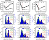 |
Fig. C.1. Results of Gaussian Mixture models for: the recent data used for this study (left column), the data set of Richardson et al. (2014) (middle column), and all data (combining both) (right column). The top row shows the BIC and AIC for models of N components, and the red dotted vertical line denotes the N that minimises BIC. The middle row shows the GMM results for N = 2 and the bottom row shows the results for N = 3. |
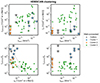 |
Fig. C.2. Scatter plots of the well-connected events in the recent data set used for this study, as a function of flare intensity for 100 keV electron intensity (top, left), 25 MeV proton intensity (top, right), and 100 keV electron to 25 MeV proton ratio (bottom right), and scatter plot of 100 keV electron to 25 MeV proton ratio versus 25 MeV proton intensity (bottom left). The observations are colour-coded according to the results of the HDBSCAN clustering analysis. The grey points denote points that the algorithm deemed as outlier points. The lines connect observations associated with the same flare. |
All Tables
Spearman correlation coefficients (p-values) for different correlations studied.
Flares, CMEs, and Type II radio bursts associated with the analysed SEP events.
All Figures
|
Fig. 1. Classification of an SEP event on April 20, 2022, based on the magnetic connections of the space craft considered in this study relative to the flare location. The green, pink, and orange sectors are the sectors of well connected, poorly connected eastern, and poorly connected western events, respectively, with reference to the flare location. The spiral magnetic field lines passing each spacecraft location are indicated by different colours and numbers. L1 (black/number 5) is well connected, and Solar Orbiter (blue/number 4) and Parker Solar Probe (purple/number 3) are poorly connected in the sector of eastern events. BepiColombo (orange/number 2)) and STEREO A (red/number 1) are poorly connected in the sector of western events. The figure is produced with the Solar-MACH tool (Gieseler et al. 2023). |
| In the text | |
|
Fig. 2. Peak intensities of ∼100 keV electrons (top panels), and 1 MeV electrons (bottom panels) as a function of ≥25 MeV proton peak intensities for well-connected events (left), western events (middle), and eastern events (right). Red triangles, blue circles, black squares, orange crosses, and purple plus symbols indicate the STEREO A, Solar Orbiter, L1, BepiColombo, and PSP observations, respectively. Large starred points following the same colour scheme highlight events that deviate from the linear trend. Small starred points represent the measurements of the same events by other spacecraft that are more consistent with the linear trend. Encircled points indicate events where no DM type II radio burst was reported. Error bars represent the error in heliocentric radial scaling measurements. CCs are provided in the legend boxes with the first value denoting the correlation coefficient, and the second (in parentheses) giving the p-value. For the well-connected events, two CCs are provided: CCall for all the events in the scatter plot, and CC∼* for the rest of the events, excluding the starred (both large and small) points. The histograms along the vertical axes show the distribution of electron peak intensities, and those along the horizontal axes show the distribution of proton peak intensities. |
| In the text | |
|
Fig. 3. Electron-to-proton peak intensity ratios for ∼100 keV electrons (top panels), and 1 MeV electrons (bottom panels) as a function of peak intensities of ≥25 MeV protons for well-connected (left), western (middle), and eastern (right) events. All symbols are the same as in Fig. 2. Large starred points highlight the group of events with high e/p ratios that lie above the linear trend in Figure 2, while the small starred points that lie on the linear trend represent the observations from same events (large starred points) taken at some other spacecraft. |
| In the text | |
|
Fig. 4. Peak intensities of ∼100 keV electrons as a function of peak intensities of 1 MeV electrons for well-connected (left), western (middle), and eastern (right) events. All symbols are the same as in Fig. 2. CCall and CC∼* are the Spearman correlation coefficient along with the p-value, for all the events in scatter plot, and for the rest of the events, excluding the starred points, respectively, for well-connected events (left) and for poorly connected events (middle and right). |
| In the text | |
|
Fig. 5. Histograms showing the distribution of the ratio of ∼100 keV to 1 MeV electron peak intensities for well-connected (top), western (centre), and eastern (bottom) events. |
| In the text | |
|
Fig. 6. Histograms of peak intensities of ∼25-MeV proton events based on an extended version (Richardson 2024) of the SEP event catalogue of Richardson et al. (2014) for well-connected (top), and poorly connected (bottom) events during December 2006 – January 2023. |
| In the text | |
|
Fig. 7. Peak intensities of SEPs as a function of flare intensity for ∼100 keV electrons (top panel), 1 MeV electrons (central panel) and ≥25 MeV protons (bottom panel) for well-connected (left), western (middle), and eastern (right) events. All symbols are same as in Fig. 2. CCall and CC∼* are the Spearman correlation coefficients along with p-value, for all the events in the scatter plot, and for the rest of events, excluding the starred points, respectively. CC* is the Spearman correlation coefficient along with p-value considering only the starred points in the well-connected events. Error bars along the x-axis represent the uncertainty in the estimated GOES-equivalent flare intensity in case of behind the limb flares observed by Solar Orbiter/STIX. |
| In the text | |
|
Fig. 9. Peak intensities of SEPs as a function of projected linear CME speed for ∼100 keV electrons (top panel), 1 MeV electrons (central panel), and ≥25 MeV protons (bottom panel) for well-connected (left), western (middle), and eastern (right) events. All symbols are the same as in Fig. 2. CCall and CC∼* are the Spearman correlation coefficients along with the p-values for all events in the scatter plot, and for the rest of events, excluding the starred points, respectively. |
| In the text | |
|
Fig. 8. Peak intensities of SEPs as a function of flare intensity for ∼100 keV electrons (top panel), 1 MeV electrons (central panel), and ≥25 MeV protons (bottom panel) for well-connected events. All symbols are the same as in Fig. 7. Large starred points represent some of the observations from a group of six SEP events, standing out from the linear trend, and small starred points represent the observations from the same six events with measurements taken at some other spacecraft, and fit into the linear trend. All the rest of points are represented in lighter colours to highlight the starred points only. CCall and CC∼* are the Spearman correlation coefficients along with the p-value for all the events in the scatter plot, and for the rest of the events, excluding all the starred points, respectively. CC* is the Spearman correlation coefficient along with the p-value considering only the starred (both large and small) points in the well-connected events. Error bars along the x-axis represent the uncertainty in the estimated GOES-equivalent flare intensity in the case of behind-the-limb flares observed by Solar Orbiter/STIX. |
| In the text | |
|
Fig. 10. Variation of the projected linear CME speed as compared to the flare intensity. Large starred points represent the group of events with high e/p ratios that deviate from the linear trend in blue Fig. 2, and small starred points represent the same events observed at other locations that lie on the linear trend in Fig. 2. Encircled points represent events where no DM radio type II burst is reported. Error bars along the x-axis represent the uncertainty in the estimated GOES-equivalent flare intensity in the case of behind-the-limb flares observed by Solar Orbiter/STIX. CCall displays the correlation coefficient of all the points marked by symbols (not taking into account the error bars). |
| In the text | |
|
Fig. 11. Electron peak intensities for both electron energies, that is, ∼100 keV (red symbols) and 1 MeV electrons (blue symbols), as a function of the longitudinal separation angle ΔΦ. The green, orange, and pink arrows indicate the sectors of well-connected, western, and eastern events, respectively. The top panel includes all events observed at any of the two electron energies. The central panel shows those events simultaneously observed at both electron energies, while those events only observed at one of the two energies (∼100 keV and 1 MeV) are displayed in the bottom panel. |
| In the text | |
|
Fig. 12. Variation of the onset delay time of SEP events from flare onset with respect to the longitudinal separation ΔΦ of the observer’s field line footpoint from the flare location for 1 MeV electrons (top panel), ∼100 keV electrons (central panel), and ≥25 MeV protons (bottom panel). All symbols are the same as in Fig. 2. Green, orange, and pink arrows represent the sectors of well-connected and poorly connected western and eastern events, respectively. |
| In the text | |
|
Fig. B.1. Peak intensities of 1 MeV electrons versus peak intensities of ∼100 keV electrons measured at STEREO A/SEPT & HET (top-left) and Solar Orbiter/EPT & HET (top-right) for four commonly observed events at both spacecraft. Legend boxes with corresponding colours have the values of slope and y-intercept for each fit on the scatter plots. The lower panel shows fits for the events observed by both spacecraft, with solid and dotted lines representing Solar Orbiter and STEREO A observations, respectively. |
| In the text | |
|
Fig. B.2. The alignment of STEREO A and Solar Orbiter fits achieved by adding 1 (= a factor of 10) to the logarithmic STEREO A intercepts. Solid and dotted lines represent Solar Orbiter and STEREO A observations, respectively. Legend boxes with corresponding colours give the slope and y-intercept for each fit. |
| In the text | |
|
Fig. B.3. Re-normalization applied to PSP measurements for 1 MeV (top panel) and ∼100 keV (lower panel) electrons. The left panel shows the fits applied to STEREO A and PSP data points, for 1 MeV (top panel) and ∼100 keV (lower panel) electrons. The right panel shows the results of PSP re-normalization applied to 1 MeV (top panel) and ∼100 keV (lower panel) electrons. In the right panel, orange and purple plus markers represent the PSP data points before and after the re-normalization, respectively. |
| In the text | |
|
Fig. C.1. Results of Gaussian Mixture models for: the recent data used for this study (left column), the data set of Richardson et al. (2014) (middle column), and all data (combining both) (right column). The top row shows the BIC and AIC for models of N components, and the red dotted vertical line denotes the N that minimises BIC. The middle row shows the GMM results for N = 2 and the bottom row shows the results for N = 3. |
| In the text | |
|
Fig. C.2. Scatter plots of the well-connected events in the recent data set used for this study, as a function of flare intensity for 100 keV electron intensity (top, left), 25 MeV proton intensity (top, right), and 100 keV electron to 25 MeV proton ratio (bottom right), and scatter plot of 100 keV electron to 25 MeV proton ratio versus 25 MeV proton intensity (bottom left). The observations are colour-coded according to the results of the HDBSCAN clustering analysis. The grey points denote points that the algorithm deemed as outlier points. The lines connect observations associated with the same flare. |
| In the text | |
Current usage metrics show cumulative count of Article Views (full-text article views including HTML views, PDF and ePub downloads, according to the available data) and Abstracts Views on Vision4Press platform.
Data correspond to usage on the plateform after 2015. The current usage metrics is available 48-96 hours after online publication and is updated daily on week days.
Initial download of the metrics may take a while.