| Issue |
A&A
Volume 692, December 2024
|
|
|---|---|---|
| Article Number | A180 | |
| Number of page(s) | 16 | |
| Section | Cosmology (including clusters of galaxies) | |
| DOI | https://doi.org/10.1051/0004-6361/202451238 | |
| Published online | 12 December 2024 | |
Revisiting the CMB large-scale anomalies: The impact of the Sunyaev-Zeldovich signal from the Local Universe
1
Université Paris-Saclay, CNRS, Institut d’Astrophysique Spatiale, 91405 Orsay, France
2
Univ. Lille, CNRS, Centrale Lille, UMR 9189 CRIStAL, 59000 Lille, France
3
Leibniz-Institut für Astrophysik (AIP), An der Sternwarte 16, 14482 Potsdam, Germany
4
Universitäts-Sternwarte, Fakultät für Physik, Ludwig-Maximilians Universität, Scheinerstr. 1, 81679 München, Germany
5
Max-Planck-Institut für Astrophysik, Karl-Schwarzschild-Straße 1, 85741 Garching, Germany
⋆ Corresponding author; gabriel.jung@universite-paris-saclay.fr
Received:
24
June
2024
Accepted:
24
October
2024
The full-sky measurements of the cosmic microwave background (CMB) temperature anisotropies by WMAP and Planck have highlighted several unexpected isotropy-breaking features on the largest angular scales. We investigate the impact of the local large-scale structure on these anomalies through the thermal and kinetic Sunyaev-Zeldovich effects. We used a constrained hydrodynamical simulation that reproduced the local Universe in a box of 500 h−1 Mpc to construct full-sky maps of the temperature anisotropies produced by these two secondary effects of the CMB, and we discuss their statistical properties on large angular scales. We show the significant role played by the Virgo cluster on these scales, and we compare it to theoretical predictions and random patches of the Universe obtained from the hydrodynamical simulation Magneticum. We explored three of the main CMB large-scale anomalies, that is, the lack of a correlation, the quadrupole-octopole alignment, and the hemispherical asymmetry, in the latest Planck data (PR4), where they are detected at a level similar to the previous releases. We also use the simulated secondaries from the local Universe to verify that their impact is negligible.
Key words: cosmic background radiation
© The Authors 2024
 Open Access article, published by EDP Sciences, under the terms of the Creative Commons Attribution License (https://creativecommons.org/licenses/by/4.0), which permits unrestricted use, distribution, and reproduction in any medium, provided the original work is properly cited.
This article is published in open access under the Subscribe to Open model. Subscribe to A&A to support open access publication.
1. Introduction
High-precision observations of cosmic microwave background (CMB) anisotropies in the past two decades have highlighted over a wide range of scales the Gaussian and isotropic nature of the early Universe that corresponds to a standard ΛCDM Universe with a period of inflation in the simplest models. However, on the largest angular scales, an ensemble of features that break this statistical isotropy or Gaussianity (see e.g., Schwarz et al. 2016; Abdalla et al. 2022; Aluri et al. 2023, and references therein) have been observed in the CMB temperature field of both WMAP1 and Planck (Planck Collaboration XXIII 2014; Planck Collaboration XVI 2016; Planck Collaboration VII 2020). This includes the lack of correlation anomaly (Hinshaw et al. 1996; Bennett et al. 2003; Spergel et al. 2003; Copi et al. 2007, 2009, 2015a; Gruppuso 2014), also formulated as a lack of power (Monteserin et al. 2008; Cruz et al. 2011; Gruppuso et al. 2013; Billi et al. 2019, 2024; Natale et al. 2019), the hemispherical asymmetry (Eriksen et al. 2004, 2007; Hansen et al. 2009; Hoftuft et al. 2009; Akrami et al. 2014; Adhikari 2015; Gimeno-Amo et al. 2023; Kester et al. 2024), the quadrupole-octopole alignment (de Oliveira-Costa et al. 2004; Ralston & Jain 2004; Schwarz et al. 2004; Land & Magueijo 2005; Gordon et al. 2005; Gruppuso & Gorski 2010; Copi et al. 2015b; Marcos-Caballero & Martínez-González 2019; Patel et al.2024), and the cold spot (Vielva et al. 2004; Cruz et al. 2005, 2006; Vielva 2010; Marcos-Caballero et al. 2017; Lambas et al. 2024). The occurrence of one of these so-called large-scale anomalies in CMB simulations of standard ΛCDM universes is rare, typically below the percent level, and it is even much lower when considered jointly because they mostly appear to be statistically independent (Muir et al. 2018; Jones et al. 2023). Moreover, future observations of these large cosmological scales will improve the statistical significance of these anomalies, for example, in the CMB polarization field (see e.g., Dvorkin et al. 2008; Mukherjee & Souradeep 2016; Billi et al. 2019; Chiocchetta et al. 2021; Shi et al. 2023, including some analyses of the Planck polarization data) with the satellite LiteBIRD2 (Suzuki et al. 2018), or in the Cosmological Gravitational Wave Background (Galloni et al. 2022, 2023) with LISA3 (Amaro-Seoane et al. 2017; Barausse et al. 2020), and they will help us to determine whether they are signatures of unknown physics.
Many of these primordial signatures have been studied. Recent works include scale-dependent primordial non-Gaussianity (Schmidt & Hui 2013; Byrnes & Tarrant 2015; Ashoorioon & Koivisto 2016; Adhikari et al. 2016, 2018; Byrnes et al. 2016; Hansen et al. 2019), direct-sum inflation (Kumar & Marto 2022; Gaztañaga & Kumar 2024), cosmic bounces (Agullo et al. 2021a,b), cosmic strings (Jazayeri et al. 2017; Yang et al. 2019), or loop quantum cosmology (Agullo et al. 2021b). However, before any detection of a primordial signature can be claimed, it is necessary to fully characterize the different foregrounds that can leave an imprint on the large-scale temperature fluctuations in the CMB. At the level of the local large-scale structure (LSS), the presence of an unknown foreground has been claimed by Luparello et al. (2022) based on a cross correlation of Planck and 2MRS4 data (see however Addison 2024, for a discussion about the significance of this detection). Around large spiral galaxies of the nearby Universe (z < 0.02), the CMB temperature decreases significantly. Moreover, the overall corresponding signal reconstructed empirically seems to reproduce the low multipole behavior of the CMB map (Hansen et al. 2023) and might even account for the cold spot (Lambas et al. 2024). More generally, the local LSS has been shown to contain its own features that deviate from the cosmic mean, with a pancake shape structure with a radius of ∼100 Mpc (Böhringer et al. 2021), an asymmetry between the northern and southern galactic hemispheres in stellar mass density (Karachentsev & Telikova 2018), and an underdensity of up to 200 Mpc (Whitbourn & Shanks 2014), except in our very close neighborhood (∼20 Mpc) because of the Virgo cluster.
It is very challenging to understand the extent to which these different anisotropic features of the local Universe can impact the CMB fluctuations. A powerful tool for approaching this issue are constrained cosmological simulations, which can accurately reconstruct the local LSS and its physical properties. An extensive body of literature is devoted to generating these constrained simulations with advanced N-body and hydrodynamical descriptions (see Vogelsberger et al. 2020, for a review) and initial conditions reconstructed from galaxy observations (see e.g., Bertschinger & Dekel 1989; Kravtsov et al. 2002; Kitaura & Enßlin 2008; Lavaux 2010; Jasche & Wandelt 2013; Wang et al. 2013; Heß et al. 2013; Sorce et al. 2014, 2016; McAlpine et al. 2022). The objective is to obtain a complete description of the distribution of matter and its properties, consistent with the known local LSS. The recent constrained hydrodynamical simulation called SLOW, generated from the initial conditions of Sorce (2018) with its large volume (500 h−1 Mpc) and realistic baryonic physics as described in Dolag et al. (2023), enables detailed analyses of its different components, such as the synchrotron emission (Böss et al. 2023) and the galaxy cluster properties (Hernández-Martínez et al. 2024).
In this work, we focus on the CMB secondary anisotropies related to the Sunayev-Zeldovich (SZ) effect (Zeldovich & Sunyaev 1969; Sunyaev & Zeldovich 1972, 1980a,b) from the local Universe. We produce high-resolution full-sky maps of its two components, the thermal (tSZ) and kinetic (kSZ) component, derived from the distribution of hot baryonic gas in the SLOW simulation. We characterize these maps first by measuring their power spectrum, which we compare to predictions from the standard halo model and to the outputs from previous hydrodynamical simulations, namely Magneticum (Dolag et al. 2016) and Coruscant Dolag et al. (2005). We evaluate the role of the nearby Virgo cluster with particular care. On large angular scales, both the kSZ and tSZ signals are significantly dominated by the structures from the very local Universe, meaning that they can carry some anisotropic large-scale features of the local LSS. We investigate their correlation with several well-known CMB large-scale anomalies, namely the lack of correlation, the quadrupole-octopole alignment, and the hemispherical asymmetry. Moreover, we apply the analysis pipeline we developed to study these anomalies to the latest Planck data release (PR4) (Planck Collaboration Int. LVII 2020) to confirm their presence at the levels reported in previous releases. This work is complementary to the analyses of Gimeno-Amo et al. (2023) and Billi et al. (2024), and it is based on the same dataset.
This paper is organized as follows. In Sect. 2 we describe our simulated maps of the thermal and kinetic SZ effects from the local Universe. In Sect. 3 we recall different estimators of several CMB large-scale anomalies, and we apply them to the latest Planck data (PR4). In Sect. 4 we characterize the statistical properties of the local tSZ and kSZ maps by studying their power spectra for the first time, and we examine the extent to which they can contribute to the CMB large-scale anomalies. Finally, we draw our conclusions in Sect. 5.
2. Data and simulations
2.1. Hydrodynamical simulations
To construct the tSZ and kSZ signals from the local Universe, we used several hydrodynamical simulations that we present in this section. Our baseline simulation was SLOW, which is a recent and large constrained hydrodynamical simulation. We compared it to two other simulations that were studied in detail in the literature: the smaller constrained simulation Coruscant, and the unconstrained Magneticum. We compare our results with these simulations to verify the impact of improvements in reconstructing the local LSS, and to determine how it differs from an average patch of our ΛCDM Universe.
2.1.1. The SLOW constrained simulation
SLOW is a hydrodynamical simulation that reproduces the CMB large-scale anomalies of the local Universe in a box of 500 h−1 Mpc. It contains 2 × 15363 dark matter and gas particles and assumes a Planck-like cosmology (see Table 1). For a detailed description of its production, we refer to Dolag et al. (2023), Hernández-Martínez et al. (2024) and references therein. We summarize the most important steps below.
Cosmological parameters of the SLOW simulation.
The key ingredient of constrained simulations is the initial conditions, which are reconstructed from observations of the local Universe using different methods. For SLOW, the initial conditions are derived following the approach described in Sorce (2018). They are based on the use of galaxy peculiar velocities that were derived from the CosmicFlows-2 data (Tully et al. 2013) to trace the full matter distribution. Larger and more recent datasets such as CosmicFlows-3 and 4 (Tully et al. 2016, 2023), which include CosmicFlows-2, have been produced. While an anomalous bulk flow was recently reported both by Whitford et al. (2023) and Watkins et al. (2023) in CosmicFlows-4, we stress that all data are fully compatible with each other and with the CosmicFlows-2 mean bulk flow value, as shown in Fig. 14 of Whitford et al. (2023). As a consequence, we also expect the initial conditions derived from CosmicFlows-2, -3, and -4 to agree with each other.
After the initial conditions were reconstructed from the galaxy peculiar velocities, they were evolved using the code OPENGADGET3 (Groth et al. 2023), which was developed from the standard TreeParticleMesh code GADGET3 (Springel 2005) with an improved smooth particle hydrodynamics solver (Beck et al. 2016). In addition to the standard gravitational evolution, the physics of baryonic matter (e.g., cooling, star formation, winds, and feedback from active galactic nuclei) is included through advanced subgrid models that were previously validated with the Magneticum hydrodynamical simulation; see Sect. 2.1.3.
Several constrained numerical simulations that used the initial conditions reconstructed from the CosmicFlows-2 dataset were produced, and comparisons with observations conducted at different scales showed that they reproduced the properties of the local Universe. At the scale of our galaxy, (e.g., Carlesi et al. 2016) showed that the local large structure induces the pair formation of the Milky Way and Andromeda. At the scale of galaxy clusters, replicas of nearby clusters such as Virgo, Centaurus, Hydra, and Perseus were studied in detail by Sorce et al. (2016, 2021), Sorce & Tempel (2018), Sorce (2018), Lebeau et al. (2024). At larger scales, the filaments connected to the Coma cluster were recovered (Malavasi et al. 2023), and velocity waves associated with the massive clusters of our local environment were shown to agree with data (Sorce et al. 2024).
The baseline-constrained simulation we used, SLOW, was also tested against observations. A large number of the most massive observed galaxy clusters were cross identified in SLOW and were found to be close to their actual position in the sky. The masses were within the observational uncertainties (Hernández-Martínez et al. 2024). On larger scales, the observed overdensity of massive galaxy clusters up to 100 Mpc and the underdensity of galaxy clusters in the same sphere, as well as the asymmetries between southern and northern directions, are also well reproduced in the SLOW simulation (Dolag et al. 2023).
2.1.2. The Coruscant constrained simulation
We considered another constrained simulation, called Coruscant, which focuses on the very local Universe. It describes the local structures in a sphere with a radius of ∼110 Mpc that is embedded in a box of size ∼240 h−1 Mpc and contains about 108 million particles in total (gas and dark matter). The initial conditions were reconstructed from the observed galaxy density field in the IRAS5 1.2-Jy survey (Fisher et al. 1995).
A first version of the simulation was described in detail in Dolag et al. (2005) (see also for an earlier work based on similar initial conditions in the dark matter only case Mathis et al. 2002), and was later updated to include an earlier version of all the ingredients also used the Magneticum simulation (for other works that analyzed this most recent version of the Coruscant simulation, see, e.g., Planck Collaboration XL 2016; Dolag et al. 2016; Coulton et al. 2022).
2.1.3. The Magneticum simulation
The final hydrodynamical simulation we studied is Box2 of the Magneticum simulation6. Its unconstrained initial conditions consist of 2 × 15843 dark matter and gas particles in a box with a size of 352 h−1 Mpc, and the run includes the ingredients of baryonic physics detailed in Hirschmann et al. (2014), Dolag et al. (2016).
2.2. tSZ and kSZ maps of the local Universe
The CMB large-scale anomalies of the Universe leaves imprints on the CMB anisotropies through different effects (for a review, see e.g., Aghanim et al. 2008). One of the most important imprints is the thermal SZ effect (Zeldovich & Sunyaev 1969; Sunyaev & Zeldovich 1972). It consists of the inverse-Compton scattering of CMB photons by electrons in the ionized gas and is mainly located in galaxy clusters. It is noted tSZ. The tSZ effect is proportional to the integral of the electron gas pressure along the line of sight. This corresponds to a spectral distortion of the CMB temperature fluctuations, which can be written as
where g(ν) is an overall factor depending on the frequency ν, and the Compton-y parameter describes the signal over the sky. These terms are given by
where h is the Planck constant, kB is the Boltzmann constant, TCMB is the CMB temperature, c is the speed of light, and σT is the scattering cross section. The electron gas pressure is Pe = kBneTe, where Te, ne, and me are the electron temperature, density, and mass, respectively.
The kinetic SZ (kSZ) effect (Sunyaev & Zeldovich 1980a,b) is induced by the bulk motion of the electron gas that moves with a peculiar velocity ve in the direction of the line of sight. It can be written as
The kSZ effect has the same blackbody dependence as the CMB primary fluctuations. In amplitude, it is dominated by its tSZ counterpart, except when the tSZ effect is null at a frequency of about 220 GHz.
Using the numerical code SMAC7 (Dolag et al. 2005), we can directly evaluate the integrands in Eqs. (2), (3) throughout the SLOW-constrained hydrodynamical simulation for a HEALPix tessellation scheme. This allows us to perform the integral in a range that is limited by the simulation volume. It is also possible to push the integration further, for example, to compute the full SZ signal. This requires generating light cones from the simulation (see Dolag et al. 2016, for an example based on the Magneticum simulation). However, we are only interested in the SZ signal from the local Universe, and we restricted the computations to the volume of the SLOW simulation.
To obtain maps of the local tSZ (Compton-y) and kSZ signals, we started the integration from the observer position, which was chosen so that the position of the largest simulated structures on the sky mimicked that of their observed counterparts as much as possible8. By construction of the constrained initial conditions, the observer position is very close to the center of the SLOW box. Then, to take advantage of the full constrained volume, we performed the integration up to 350 Mpc around it (the maps we obtained are referred to as SLOW-350). We also generated maps focused on the closest structures, up to 110 Mpc (constrained volume of Coruscant), from SLOW (the maps we obtained are referred to as SLOW-110) and Coruscant, both for comparison between the two generations of constrained simulations and for the direct study of close-by structures while avoiding contamination from the background. These maps have a resolution of Nside = 1024 (pixels with a size of ∼3.4 arcmin) and constitute the core ingredient of this paper. They are shown in Fig. 1.
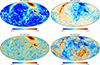 |
Fig. 1. tSZ (y-Compton) and kSZ signals from the local Universe in the SLOW constrained simulation. The upper panels only include the most local structures (up to 110 Mpc, denoted SLOW-110), and the lower panels use almost the full volume of the box (up to 350 Mpc, denoted SLOW-350). The color scale is logarithmic in the tSZ maps and symmetric logarithmic for the kSZ maps. The main characteristics of these maps are recalled in Table 2. |
Characteristics of the tSZ and kSZ maps constructed from the SLOW, Magneticum and Coruscant hydrodynamical simulations.
On the largest scales, these maps are highly anisotropic as the signal is dominated by a few extended structures from the very local Universe. The most prominent structure, located in the upper right corner of each plot, corresponds to the Virgo galaxy cluster. It leads to a large positive (negative) contribution in the tSZ (kSZ) maps, respectively. Several other well-known galaxy clusters can be cross-identified in this simulation, with a good match of position and mass, as discussed in detail in Hernández-Martínez et al. (2024).
The observed and simulated positions of these clusters in the sky differ slightly, however, as does their distance from the observer. These differences are mainly due to intrinsic limitations of the initial conditions reconstruction method, which causes structures to be slightly displaced with respect to their expected position. These differences in the position of the structures may also arise when the reconstructed initial conditions are based on different datasets, which leads to slightly different values of the bulk flow. To estimate the impact of these differences, we produced a set of maps (SLOW-near) in which the observer position was shifted 1 Mpc in different directions (14 new positions per maps) in the SLOW box. We also tested a larger displacement of 2 Mpc, which produced very similar conclusions.
Finally, to verify how the local tSZ and kSZ signals compare to random patches of the Universe, we generated sets of maps in which the observer positions were selected in very distant positions (more than 100 Mpc between each) in both SLOW (SLOW-grid) and Magneticum (27 maps for each). This allowed us to obtain almost independent realizations of the SZ signals.
A list of the different maps and of their main characteristics is given in Table 2. Their statistical properties are discussed in detail in Sect. 4.
2.3. Planck CMB data
For the analyses presented in Sect. 3, we used the CMB temperature datasets from the latest Planck release (for details about the PR4 release, see Planck Collaboration Int. LVII 2020). They include foreground-cleaned CMB maps produced by the component separation methods SEVEM (Fernandez-Cobos et al. 2012) and Commander (Eriksen et al. 2008). They are available at the Planck Legacy Archive9 (PLA). We also used the associated simulated CMB maps (600 and 100 for SEVEM and Commander, respectively), which are accessible from the National Energy Research Scientific Computing Center (NERSC)10.
The main mask we used is the 2018 Planck common mask. In addition, to confirm the robustness of our results against astrophysical contamination, we also considered masks covering a larger area near the galactic plane. All these masks can be found in the PLA.
We are primarily interested in large-scale effects and therefore did not work directly with the data at full resolution (Nside = 2048, and a Gaussian beam with an FWHM of 5′). We instead used a downgraded resolution (Nside = 64, and 160′ Gaussian beam), as in Planck Collaboration VII (2020). A map with this low resolution and large beam washes out small-scale variations of the signal, in particular, the variation that is associated with structures such as clusters of galaxies. This leads to a negligible impact on the overall CMB signal at large scales. After downgrading, we set all pixels with a value below 0.95 to 0 for the masks to maintain their binarity.
Before we estimated the different statistics of interest introduced in the following section, the masks were applied to the CMB Planck data maps and their simulated counterparts. We then removed the monopole and dipole of the resulting masked maps. This removed any large-scale coherent signal such as that potentially associated with a large-scale bulk flow. As the mask itself can have a strong impact on the large-scale statistics we measured, it was necessary to fill in the masked regions. We used the diffusive inpainting technique (see for example Gruetjen et al. 2017, for details).
3. Large-scale anomalies in Planck CMB data
In this section, we investigate several well-studied large-scale anomalies of the CMB temperature anisotropies using the most recent data available from Planck (PR4; see Sect. 2.3 for details). For each anomaly, we briefly recall the historical definition and a corresponding standard estimator before we apply it to the Planck observed and simulated CMB maps.
3.1. Lack of correlation
One surprising feature of the CMB anisotropies that was first observed in COBE11 data (Hinshaw et al. 1996) is that the two-point angular correlation function C(θ) (2PACF) seems to vanish on large angular scales (θ > 60°). To quantify this so-called lack of correlation, the standard choice of statistics is the quantity noted S1/2. It is written as
![$$ \begin{aligned} {S\!}_{1/2} \equiv \int _{-1}^{1/2} \left[C(\theta )\right]^2 \mathrm{d} (\cos \theta ). \end{aligned} $$](/articles/aa/full_html/2024/12/aa51238-24/aa51238-24-eq4.gif)
It was originally introduced in (Spergel et al. 2003) and has been used in many works based on WMAP or Planck data (see for example Copi et al. 2007, 2009, 2015a; Gruppuso 2014; Schwarz et al. 2016; Planck Collaboration XXIII 2014; Planck Collaboration XVI 2016; Muir et al. 2018; Planck Collaboration VII 2020; Jones et al. 2023). We follow the computation steps of Copi et al. (2009), who evaluated S1/2 directly from (pseudo-) power spectrum measurements.
To estimate this pseudo-Cℓ from the Planck CMB maps, we used the numerical code NaMaster12 as described in Alonso et al. (2019) (for earlier works on pseudo-Cℓ estimation, see Wandelt et al. 1998; Hivon et al. 2002; Hansen et al. 2002; Tristram et al. 2005). With this method, which was constructed to handle masked maps, we did not need to perform the inpainting step after applying the Planck common mask.
Our results are shown in Fig. 2. As is known since COBE observations (Bennett et al. 1993), which were later confirmed in WMAP data (Spergel et al. 2003), the observed quadrupole has a low amplitude that is one of the lowest in the simulations (2.5% and 5% of the lowest in SEVEM and Commander simulations, respectively). The octopole moment is also rather low (15th percentile). This cannot be considered as anomalous, however, as was shown in (Efstathiou 2003), and it does not explain the lack of correlation effect by itself.
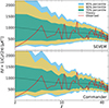 |
Fig. 2. Pseudo-Cℓ of the Planck PR4 CMB temperature maps from SEVEM (top panel) and Commander (bottom panel). The solid red lines are measured from cleaned observed maps, and the dotted black lines are theoretical predictions computed using CAMB. The colored areas are determined from simulations and show their distribution around the median. For the two component separation methods, the observed quadrupole belongs to the lowest 5% of the simulated values (only 15 SEVEM simulations out of 600 have a lower quadrupole, and 4 for Commander). Only 15% of the simulations have a smaller octopole. |
In Fig. 3, we show the quantity S1/2 computed from the Planck PR4 pseudo-Cℓ of Fig. 2. The observed value is clearly lower than in all the simulations. This confirms that the 2PACF is anomalously close to zero on angular scales (θ > 60°).
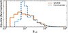 |
Fig. 3. Lack of correlation on large angular scales (θ > 60°) in the cleaned Planck PR4 CMB temperature maps. We show the distribution of the statistic S1/2 (Eq. (4)) measured in the Planck PR4 simulations, and the vertical lines (on the left) are the observed values. The dashed blue and solid orange lines correspond to the Commander and SEVEM maps, respectively. None of the measured S1/2 in the simulations is as low as in the observations. |
3.2. Alignment of the quadrupole and octopole
Another striking feature of the CMB temperature fluctuations is the alignment of the quadrupole and octopole (first reported in WMAP data de Oliveira-Costa et al. 2004), which can be studied using multipole vectors (Maxwell 1865; Copi et al. 2004; Dennis 2004). These multipole vectors constitute an alternative to the standard decomposition of CMB anisotropies into spherical harmonics, where the information contained in each multipole ℓ is given by a real constant and ℓ unit vectors vℓj (with j = 1⋯ℓ).
To estimate low-ℓ multipole vectors in the Planck PR4 maps, we used the optimized numerical code polyMV13 presented in Oliveira et al. (2020). We then followed the analyses of Schwarz et al. (2004), Copi et al. (2006) where the key ingredient for studying alignments is the area vectors, which are defined as cross-products between multipole vectors at a given ℓ,
There is thus one vector w2 for the quadrupole, corresponding to one preferred direction, and three vectors (w31, w32, and w33) for the octopole. To measure the alignment of the octopole with any given direction in the sky Ω, we can compute the following quantity:
We are interested in two specific values of S(Ω): its maximum, and S(w2). We denote them SO and SQO in the following. The first value measures the alignment of the three area vectors of the octopole and defines its averaged preferred direction, and the second value estimates the alignment between the quadrupole and octopole.
In Fig. 4 we show the distribution of SO and SQO determined from the Planck PR4 simulated maps and their observed counterparts. Only 10% of the simulations have a higher value of SO, which confirms that its three area vectors are relatively well aligned. This is the so-called planarity of the octopole. By itself, this does not constitute an anomaly, but it allows the high value of SQO, which is very close to SO. An alignment of the quadrupole and octopole like this is only found in one of the simulated CMB maps of each set.
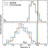 |
Fig. 4. Quadrupole-octopole alignment in the cleaned Planck PR4 CMB temperature maps. In the upper panel, we show the distribution of SO (see Eq. (6)), indicating the planarity of the octopole is. Higher values are obtained for 59 SEVEM simulations (out of 600) and 9 (out of 100) for Commander. In the lower panel, we show the distribution of SQO, measuring the alignment between quadrupole and octopole. Only one simulation in both sets has a higher SQO value than the observed data. The solid orange and dashed blue lines correspond to the SEVEM and Commander maps, respectively. |
In Fig. 5 we show the preferred directions of the quadrupole and octopole as determined from the Planck PR4 CMB maps after applying the common mask and inpainting the masked areas, as described in Sect. 2.3. As expected from the measured values of SQO, the two favored axes point to the same area of the sky. The corresponding direction is close to the ecliptic plane and points toward the position of the Virgo cluster.
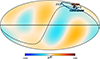 |
Fig. 5. Quadrupole-octopole alignment in the cleaned Planck PR4 CMB temperature maps. The preferred direction of the quadrupole is given by the orange circle and blue crosses for SEVEM and Commander, respectively. The orange and blue contours, which are almost superimposed, correspond to the areas where S(Ω) (defined in Eq. (6)) is within 3% of its maximum (preferred direction of the octopole), for SEVEM and Commander respectively. The background map is the sum of the SEVEM CMB quadrupole and octopole. The solid and dashed black lines correspond to the galactic and ecliptic planes, respectively. We only show the preferred directions in the northern galactic hemisphere. |
3.3. Hemispherical asymmetry
An efficient method for studying large-scale anisotropies of the CMB are position-dependent statistics. This consists of dividing the sky into a set of equal-size and uniformly distributed patches, and then computing patch by patch a chosen statistic for measuring its variation over the celestial sphere. Depending on the considered statistics as well as the patch properties (e.g., size and shape), different physical effects and scales can be probed.
For example, simply measuring the pixel variance in each patch is a very powerful probe of the hemispherical asymmetry (known since WMAP; see e.g. Eriksen et al. 2004). This position-dependent variance (or local-variance) estimator was originally introduced by Akrami et al. (2014), and was applied to the different releases of Planck data (for a recent analysis of the PR4 data, see Gimeno-Amo et al. 2023). We extended the analysis to higher-order moments, namely the skewness and kurtosis. In Appendix A we also compute the position-dependent power spectrum.
Our patches were constructed from a very low resolution HEALPix map (Nside = 8) by setting one pixel to one and the rest to zero, and by upgrading its resolution to the same resolution as for the maps we analyzed (here Nside = 64). Repetition of the process for each pixel of the low-resolution maps produced a set of 768 patches that covered the full sky, without any overlapping areas. In Appendix B we repeat our analysis considering disks with a radius of 4°, which is the main patch choice of Planck Collaboration VII (2020), Gimeno-Amo et al. (2023). Both sets lead to the similar conclusions, with a higher statistical significance for the disks that were fine-tuned to study the hemispherical asymmetry.
We measured the temperature variance in patches of the Planck PR4 CMB maps at low resolution (and the simulated CMB maps) after applying the common mask. Patches with more than 90% of masked pixels were excluded following the analysis of Planck Collaboration VII (2020). For each patch of every map, we then subtracted the average value and divided by the variance computed from the corresponding set of simulations. The resulting maps are called position-dependent variances in the rest of the section. Position-dependent skewness and kurtosis maps were obtained following the same method.
To verify the presence of any hemispherical asymmetry, we fit a dipole to these position-dependent variances (and higher-order moments). Its amplitude Ad can confirm or refute the presence of an asymmetry in the maps, and its direction is orthogonal to the plane defining the two hemispheres. In Table 3, we compare the data dipole amplitude to the simulations, and we verify the well-known result that in the variance case, it is larger than for the vast majority of the simulated CMB maps at the 1 − 2% level. No dipolar asymmetry is observed for the skewness and kurtosis. In Fig. 6 we then show the corresponding directions on the sky of the position-dependent variance dipoles. The dipole directions of the different simulated CMB maps point all over the sky, which confirms that there is no preferred axis inherent to our analysis pipeline (e.g., masking choices). The observed asymmetry axis is relatively close to the supergalactic plane, where many CMB large-scale anomaliess of the local Universe can be observed (e.g., the Virgo, Coma, Centaurus, or Perseus clusters). In Sect. 4.2 we apply the same method to the local Universe simulations to determine whether its tSZ and kSZ contributions can explain the observed asymmetry.
Dipole amplitude of position-dependent statistics.
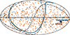 |
Fig. 6. Preferred direction of the variance asymmetry in the Planck PR4 CMB temperature maps. Dipoles are computed from the position-dependent variance maps computed using HEALPix pixel patches. The data dipole directions are given by the large blue crosses and orange disks for Commander and SEVEM, respectively, and the small markers are for the corresponding simulations. The blue and orange lines are the planes orthogonal to these observed dipoles. The solid, dashed and dash-dotted lines correspond to the galactic, ecliptic and supergalactic planes, respectively. |
Finally, we used the plane orthogonal to the measured dipole of each position-dependent statistics map in order to separate the map into two hemispheres, and we averaged it over these two halves of the sky. The results are shown in Fig. 7, where we compare the distribution of the different averaged quantities over the full sky, and the hemispheres in the dipole direction and opposite to it. In the direction opposite to the dipole in the observed data (close to the supergalactic northern hemisphere), the position-dependent variance is very low (among the 3% lowest CMB simulated maps for the disks, as verified in Appendix B), while the other hemisphere does not show any deviation. A splitting of the sky into two halves on either side of the ecliptic plane gives similar results, with a very low variance in one of the hemispheres. For the skewness, no such effect is seen, and this is also the case when splitting the sky using the ecliptic or supergalactic planes. In the Planck map obtained from Commander,, we observe a large position-dependent kurtosis, even in the full-sky case, and with a non-negligible difference with the SEVEM results. We verified that the excess is localized in the supergalactic and ecliptic southern hemispheres, but no specific source can be easily identified. While there is a difference between the two hemispheres, no strong dipolar modulation was detected for the kurtosis, as reported in Table 3, and thus, we cannot directly relate this issue with the hemispherical asymmetry anomaly.
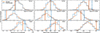 |
Fig. 7. Hemispherical asymmetry in the Planck PR4 CMB temperature data. From left to right, we show the position-dependent variance, skewness, and kurtosis averaged over the full sky (upper row), and the two hemispheres defined by the plane orthogonal to the position-dependent variance of each individual map (opposite and same directions as the dipole in the middle and lower rows, respectively). The vertical orange and blue lines correspond to the observed SEVEM and Commander maps, respectively, and the histograms were obtained from the corresponding 600 SEVEM (orange), and 100 Commander (blue) simulations. There is a lack of variance in the hemisphere opposed to the dipole, where 583 (out of 600) SEVEM and 99 (out of 100) Commander simulations have higher values than the data. |
4. Characterizing the tSZ and kSZ effects from the local Universe
In this section, we further explore the statistical large-scale properties of the tSZ and kSZ effects from constrained simulations of the local Universe. In the first part, we focus on the power spectrum, and in the second part, we evaluate the impact of the secondary anisotropies induced by the local Universe on the different large-scale CMB anomalies studied in Sect. 3.
4.1. SZ power spectra from the local Universe
We measured power spectra from the different maps shown in Fig. 1 (see also Table 2). This included tSZ and kSZ maps for the two volumes of the local Universe (rmax = 110, 350 Mpc) and rmax = 110 Mpc maps, in which the position of the observer is slightly or strongly displaced in the SLOW simulation. As expected, the tSZ signal was stronger by about one magnitude and dominated its counterpart kSZ effect at all scales.
For comparison purposes, we computed theoretical predictions for the tSZ power spectrum using the emulator described by Douspis et al. (2022), trained on the halo model developed by Salvati et al. (2018). We also computed these predictions for the kSZ power spectrum using the numerical code class_sz14 (Bolliet et al. 2023)15, considering three different redshift ranges for the integration (two corresponded to the local Universe volumes, and the third to an integration up to z = 4).
In Fig. 8 we compare these theoretical predictions to the power spectra from the simulated maps. We focus on the large scales (ℓ ≤ 150), where the local tSZ and kSZ effect are expected to either dominate or to contribute significantly to the full SZ signal, as verified by theoretical calculations. This shows the agreement between these theoretical predictions and the range (defined as a 90% percentile) that is spanned by the SLOW-grid set, with a few exceptions that we discuss below.
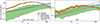 |
Fig. 8. Local tSZ (left) and kSZ (right) power spectra compared to the average. The solid red and blue lines are power spectra measured from the maps shown in Fig. 1, constructed by integrating electron gas properties through the SLOW simulation from the position of the Milky Way to rmax = 110 and rmax = 350 Mpc, respectively. The colored areas are 90% percentiles determined from the sets of maps where the center for the integration is displaced in the SLOW simulation, slightly (by 1 Mpc from the Milky Way) in orange (SLOW-near), and strongly (more than 100 Mpc between each center) in green (SLOW-grid). The dashed lines show theoretical predictions computed in the halo model, where the red and blue lines are integrated up to rmax = 110 and rmax = 350 Mpc, and the black lines correspond to the full expected tSZ or kSZ signals. The tSZ power spectrum is shown at the frequency 143 GHz. |
For ℓ ≤ 70, the tSZ power spectrum from the local Universe is well above the SLOW-grid range, and it is larger by up to one magnitude than the theoretical prediction. The small uncertainties on the position of the Milky Way in the simulation that was obtained with the SLOW-near set have a much weaker effect on this power spectrum, about 20% at most. In addition, for ℓ < 30, the tSZ signal is almost entirely due to the very local Universe (rmax = 110 Mpc map). Similarly, the kSZ contribution of the local Universe is also at the high limit of the expected range, and again, the very local Universe represents a large part of the signal.
As we verified by applying different masks, the large amplitude of the local Universe tSZ power spectrum at low ℓ is related to the simulated replica of the Virgo cluster. We applied a disk mask with a radius of 10° centered on the Virgo cluster on the local Universe tSZ and kSZ maps (tests with smaller disks showed that they were not sufficient to remove the full contribution of Virgo). Similarly, we constructed one mask for each map of the SLOW-grid and SLOW-near sets to remove the contribution of the most prominent cluster in each map. This most prominent cluster was identified with the following procedure, which consisted of downgrading the tSZ maps to a resolution of Nside = 32 and using the pixel with the highest value as the center of the disk mask. With this method, the Virgo cluster was always selected in the SLOW-near simulations, as intended.
The power spectra computed on these masked simulations of the tSZ and kSZ effects are shown in Fig. 9. When the contribution of the Virgo cluster is removed, the tSZ power spectrum at low ℓ decreases by more than one order of magnitude, bringing it in the range given by the SLOW-grid set, but it is still in the high part. When Virgo is masked, the kSZ power spectrum is brought within the average on large scales. Moreover, masking the most prominent cluster has a weaker effect on most of the simulations than in the local Universe case. It decreases the tSZ signal by a factor 2 on average. In the SLOW-grid set of 27 simulations, only one simulation had a similar decrease after masking. This confirms the low probability of having a strong contribution from a cluster that is sufficiently close and as large as Virgo is.
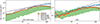 |
Fig. 9. Same as Fig. 8, where the most prominent cluster in each simulation has been masked by a disk with a radius of 10°. In the local Universe, this corresponds to the Virgo cluster. |
We also individually masked several other identified clusters of the local Universe that were identified in Hernández-Martínez et al. (2024). The only cluster that contributed significantly to the power spectrum was Centaurus, which dominated the signal around ℓ ∼ 50. In Fig. 10 we verify that masking both Virgo and Centaurus indeed removes most of the SLOW-110 tSZ and kSZ signals, and the difference with the SLOW-350 power spectra finally becomes significant. In addition, the local Universe is now at the lower end of the SLOW-grid range. This is consistent with the main conclusions of Sorce et al. (2016), Dolag et al. (2023), who reported that the simulated local Universe is underdense up to 200 Mpc, in agreement with observations (see e.g. Whitbourn & Shanks 2014). The simulated equivalent of the Centaurus cluster of SLOW has been shown by Hernández-Martínez et al. (2024) to be almost five times more massive than expected, however. This means that its simulated SZ contribution is also larger.
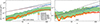 |
Fig. 10. Same as Fig. 8, where the two most prominent clusters in each simulation have been masked by a disk with a radius of 10°. In the local Universe, this corresponds to the Virgo and Centaurus clusters. |
For further comparisons, we measured the power spectra from the maps derived from the constrained Coruscant and unconstrained Magneticum hydrodynamical simulations that we presented in Sects. 2.1.2 and 2.1.3, respectively. The corresponding results are shown in Figs. 11 (full sky) and 12 (with the most prominent cluster masked, e.g., Virgo in the case of the local Universe). Due to the different characteristics of each simulation (cosmological parameters, resolution, box sizes), no perfect agreement is expected. To take the dependence on cosmological parameters into account, we rescaled the tSZ power spectra of the Coruscant and Magneticum maps using CℓtSZ ∝ σ83Ωm3 (Hill & Pajer 2013). Similarly, the Coruscant and Magneticum kSZ power spectra were rescaled using the factor between the theoretical predictions obtained for the different cosmologies.
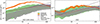 |
Fig. 11. tSZ and kSZ power spectra up to rmax = 110 Mpc from several hydrodynamical simulations. As in Fig. 8, the solid red line and the orange and green areas are determined from the SLOW simulation, and the dashed lines are the corresponding predictions from the halo model. The solid purple lines are estimated from local Universe maps determined from the Coruscant simulation, and the gray areas are 90% percentiles from the Magneticum simulation. |
One important difference between the two generations of constrained simulations (SLOW and Coruscant) is the impact of the Virgo cluster on large scales. In Coruscant, no excess signal is observed on these scales, which means that it is lower by one order of magnitude than SLOW. However, after masking Virgo, the tSZ and kSZ power spectra of both maps match extremely well up to ℓ ∼ 20 (tSZ) and ℓ ∼ 100 (kSZ), before other effects such as the resolution of the box play a role. For the kSZ power spectrum, removing the Virgo contribution also has a much stronger effect in SLOW.
Furthermore, the SLOW-grid set of maps spans a wider range of values than its equivalent set from Magneticum on large scales (ℓ ≤ 30), which indicates that a cluster like Virgo is even more unlikely in the Magneticum set (close and large enough to entirely dominate the signal). One possible explanation is that, as reported in Sorce et al. (2016), Dolag et al. (2023), the local Universe contains a significant overdensity of very massive clusters (masses above 1015 M⊙) in a large volume around our position (up to rmax = 200 Mpc) with respect to the Magneticum simulation (although not exactly the same as here). This might make a massive cluster in the neighborhood of the different centers used in the SLOW-grid set more likely.
In conclusion, this highlights two interesting properties of the local tSZ and kSZ power spectra on large scales compared to other volumes of the same size selected randomly. The local power spectra are dominated by a very low number of clusters, mainly Virgo and Centaurus. Despite this, the low-ℓ tSZ power spectrum is larger than in the majority of the other simulated maps (around 95%), mainly because the Virgo cluster is so close to us. Its signal expands on a large area of the sky, as a disk with a radius of 10° is necessary to mask it fully, which is much wider than the disk radius of 2° of the Planck common mask, for example. Therefore, we evaluate in the following section whether this larger-than-expected local SZ signal can significantly modify the statistical properties of the CMB on very large angular scales.
4.2. Local tSZ and kSZ effects and CMB large-scale anomalies
We used the simulated maps of the tSZ and kSZ effects from the local Universe, shown in Fig. 1, to investigate their impact on the largest angular scales of the CMB. On these scales, several so-called anomalies (see Sect. 3) have been observed, with indications of a correlation with the local Universe (e.g., alignments of low multipoles near the Virgo direction, or an asymmetry axis close to the supergalactic plane).
For this purpose, we produced CMB realizations including the local tSZ and kSZ effects. We started by generating 10 000 CMB Gaussian realizations from the Planck best-fit theoretical power spectrum computed with CAMB, with a resolution of Nside = 64 and a Gaussian beam with an FWHM of 160′, which is the same as for the Planck maps described in Sect. 2.3. To each of these Gaussian CMB simulations, we added the tSZ and kSZ signal from the local Universe obtained from the constrained simulations at a chosen frequency, after degrading the map resolution to Nside = 64 and applying the 160′ Gaussian beam (again, the same as for the Planck maps). We masked the galactic plane, and in some cases, Virgo (with a disk radius of 10°), keeping almost 70% of the sky for the analysis. The dipole of the resulting maps was then removed, which minimized the impact of any potential systematics at the dipole level in the initial conditions of the reconstruction procedure. Finally, we computed the different estimators of CMB large-anomalies described in Sect. 3 in the Gaussian CMB simulations and in their CMB + SZ counterparts to compare the differences.
We report our main results in Figs. 13, 14, and 15 and focus on the lack of correlation, quadrupole-octopole alignment, and hemispherical asymmetry anomalies, respectively. We used the rmax = 350 Mpc maps as our baseline, with a frequency of 143 GHz for the tSZ signal. At this frequency, the tSZ signal entirely dominates its kSZ counterpart, as shown in Sect. 4.1. Therefore, the latter is not expected to play a significant role at very large scales. Still, at galaxy cluster scales (a few to a few dozen arcminutes), kSZ can impact the total signal of individual clusters depending on the direction of their bulk velocity. Further tests with other frequencies and in particular, at 217 GHz, where the tSZ signal is suppressed, led to very similar conclusions. We also verified that the lower rmax maps and a full-sky analysis did not impact our results significantly.
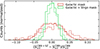 |
Fig. 13. Impact of the local Universe SZ signal on the lack of correlation at angular scales θ > 60°. We measure the difference of S1/2 (see Eq. (4)) between Gaussian CMB realizations with or without the local tSZ (at 143 GHz) and kSZ effects, when the galactic plane alone was masked (in red), and when the galactic plane and Virgo were masked (in green). The distributions are shown for both the full set (solid lines) and for the 5% (dashed) simulations where the lack of correlation is strongest (smallest S1/2). |
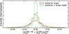 |
Fig. 14. Impact of the local Universe SZ signal on the quadrupole-octopole alignment. We measure the difference of SQO (see Eq. (6)) between Gaussian CMB realizations with or without the local tSZ (at 143 GHz) and kSZ effects, when the galactic plane alone was masked (in red), and when the galactic plane and Virgo were masked (in green). The distributions are shown for both the full set (solid lines) and the 5% (dashed) simulations where the alignment is strongest (largest SQO). |
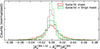 |
Fig. 15. Impact of the local Universe SZ signal on the hemispherical asymmetry. We measure the difference of Ad (amplitude of the position-dependent variance dipole; see Sect. 3.3 for details) between Gaussian CMB realizations with or without the local tSZ (at 143 GHz) and kSZ effects, when the galactic plane alone was masked (in red), and when the galactic plane and Virgo were masked (in green). The distributions are shown for both the full set (solid lines) and the 5% (dashed) simulations where the hemispherical asymmetry is strongest (largest Ad). |
The main conclusion was the same for the three anomalies. The SZ effect from the local Universe affects the different quantities by a few percent at most, which is far below the level of the anomalies. For example, the observed S1/2 is lower than half of the lowest value of all the simulated Planck CMB maps (which itself is a few times lower than the average). Similarly, moving the observed SQO by 2% would still leave it in the tail of the distribution of alignments in the simulated Planck CMB maps. Moreover, there is no visible preferred sign, meaning that its effect on the distribution of the different statistics is even much weaker on average.
When we focus on the simulations that are “anomalous” (i.e., the different estimators are in the tail of the expected distribution, at a level similar to the Planck estimators), the impact of the SZ effect from the local Universe is even smaller. The effect is slightly stronger at most when Virgo is not masked at all, meaning that despite its domination of the SZ signal at low multipoles, its effect on CMB large-scale anomalies is only very weak.
5. Conclusion
We have explored the impact of the local Universe through the tSZ and kSZ effects on the CMB temperature anisotropies at large scales. Our objective was twofold: to characterize the large-scale properties of the CMB temperature fluctuations with a new analysis of the large-scale anomalies of the latest Planck data, and to verify their correlation with the local tSZ and kSZ signals as obtained from advanced constrained hydrodynamical cosmological simulations.
Using the constrained hydrodynamical simulation SLOW to reproduce a large volume of the nearby LSS, we constructed high-resolution maps of the local tSZ and kSZ effects. We showed that they are the dominant contributions of the overall expected tSZ and kSZ effects on large angular scales by comparison to theoretical predictions, which leaves the anisotropic features correlated to the local Universe in the large-scale fluctuations of the CMB. We characterized the local tSZ and kSZ signals mainly by studying their power spectrum, highlighting their strong dependence on a few specific structures in the maps. First tests with higher-order statistics such as the bispectrum, which are beyond the scope of this work and will be discussed in future works, led to similar conclusions. In particular, the Virgo cluster causes most of the large-scale signal. Moreover, this signal is stronger than in ∼95% of the other random patches of the Universe that we tested, regardless of whether we moved the observer position in the SLOW simulation or used the unconstrained Magneticum simulation. The localization and the amplitude of the local Universe tSZ and kSZ signals, which is higher than expected, mean that further investigation of their impact on the large-scale CMB temperature fluctuations is required, for example, based on the methods developed to study the CMB large-scale anomalies.
We have analyzed several of the CMB temperature large-scale anomalies in the latest Planck temperature data (PR4), the lack of correlation using the quantity S1/2, the quadrupole-octopole alignment using multipole vectors and the hemispherical asymmetry with a local variance approach. Our analysis was conducted on cleaned CMB maps from both Commander and SEVEM and led to similar conclusions as other analyses that were conducted on previous datasets (see e.g., Planck Collaboration VII 2020, for PR3 results), or (Gimeno-Amo et al. 2023; Billi et al. 2024, on PR4). These unexpected deviations from isotropy are observed at a level found in typically less than 1% of the Planck CMB simulated maps, with some properties, such as a preferred direction of the quadrupole and octopole in the Virgo region and an asymmetry axis that is very close to the supergalactic plane. This indicates that the local LSS is a possible explanation.
We have used the simulated maps of the tSZ and kSZ effects from the local Universe, together with Gaussian CMB realizations based on the Planck best-fit cosmological parameters, to estimate the impact of these secondary anisotropies on the largest angular scales of the CMB fluctuations. Our analysis was based on the same estimators as the analysis of large-scale anomalies in the Planck data, and we showed that the local tSZ and kSZ effects cannot explain the detected deviations from isotropy.
class_sz is based on the class code http://class-code.net/ (Blas et al. 2011).
Acknowledgments
The authors thank the referee for their comments and suggestions. We thank Adélie Gorce, Andrea Ravenni and Saleem Zaroubi for useful inputs and discussions. This work was supported by the grant agreements ANR-21-CE31-0019/490702358 from the French Agence Nationale de la Recherche/DFG for the LOCALIZATION project. NA acknowledges funding from the ByoPiC project from the European Research Council (ERC) under the European Union’s Horizon 2020 research and innovation program grant number ERC-2015-AdG 695561. KD acknowledges support by the COMPLEX project from the European Research Council (ERC) under the European Union’s Horizon 2020 research and innovation program grant agreement ERC-2019-AdG 882679. The authors acknowledge the Gauss Centre for Supercomputing e.V. (www.gauss-centre.eu) for funding this project by providing computing time on the GCS Supercomputer SuperMUC-NG at Leibniz Supercomputing Centre (www.lrz.de) under the projects pr86re, pr83li and pn68na. This research made use of observations obtained with Planck (http://www.esa.int/Planck), an ESA science mission with instruments and contributions directly funded by ESA Member States, NASA, and Canada. The authors acknowledge the use of the healpy and HEALPix packages (Zonca et al. 2019; Górski et al. 2005).
References
- Abdalla, E., Abellán, G. F., Aboubrahim, A., et al. 2022, J. High Energy Astrophys., 34, 49 [NASA ADS] [CrossRef] [Google Scholar]
- Addison, G. E. 2024, ApJ, 969, 66 [NASA ADS] [CrossRef] [Google Scholar]
- Adhikari, S. 2015, MNRAS, 446, 4232 [NASA ADS] [CrossRef] [Google Scholar]
- Adhikari, S., Shandera, S., & Erickcek, A. L. 2016, Phys. Rev. D, 93, 023524 [NASA ADS] [CrossRef] [Google Scholar]
- Adhikari, S., Deutsch, A.-S., & Shandera, S. 2018, Phys. Rev. D, 98, 023520 [NASA ADS] [CrossRef] [Google Scholar]
- Aghanim, N., Majumdar, S., & Silk, J. 2008, Rep. Prog. Phys., 71, 066902 [NASA ADS] [CrossRef] [Google Scholar]
- Agullo, I., Kranas, D., & Sreenath, V. 2021a, Gen. Rel. Grav., 53, 17 [NASA ADS] [CrossRef] [Google Scholar]
- Agullo, I., Kranas, D., & Sreenath, V. 2021b, Front. Astron. Space Sci., 8, 703845 [CrossRef] [Google Scholar]
- Akrami, Y., Fantaye, Y., Shafieloo, A., et al. 2014, ApJ, 784, L42 [NASA ADS] [CrossRef] [Google Scholar]
- Alonso, D., Sanchez, J., & Slosar, A. 2019, MNRAS, 484, 4127 [Google Scholar]
- Aluri, P. K., Cea, P., Chingangbam, P., et al. 2023, Class. Quant. Grav., 40, 094001 [NASA ADS] [CrossRef] [Google Scholar]
- Amaro-Seoane, P., Audley, H., Babak, S., et al. 2017, ArXiv e-prints [arXiv:1702.00786] [Google Scholar]
- Ashoorioon, A., & Koivisto, T. 2016, Phys. Rev. D, 94, 043009 [NASA ADS] [CrossRef] [Google Scholar]
- Barausse, E., Berti, E., Hertog, T., et al. 2020, Gen. Rel. Grav., 52, 81 [NASA ADS] [CrossRef] [Google Scholar]
- Beck, A. M., Murante, G., Arth, A., et al. 2016, MNRAS, 455, 2110 [Google Scholar]
- Bennett, C. L., Boggess, N. W., Cheng, E. S., et al. 1993, Adv. Space Res., 13, 409 [NASA ADS] [CrossRef] [Google Scholar]
- Bennett, C. L., Halpern, M., Hinshaw, G., et al. 2003, ApJS, 148, 1 [Google Scholar]
- Bertschinger, E., & Dekel, A. 1989, ApJ, 336, L5 [NASA ADS] [CrossRef] [Google Scholar]
- Billi, M., Gruppuso, A., Mandolesi, N., Moscardini, L., & Natoli, P. 2019, Phys. Dark Univ., 26, 100327 [NASA ADS] [CrossRef] [Google Scholar]
- Billi, M., Barreiro, R. B., & Martínez-González, E. 2024, JCAP, 07, 080 [Google Scholar]
- Blas, D., Lesgourgues, J., & Tram, T. 2011, JCAP, 07, 034 [CrossRef] [Google Scholar]
- Böhringer, H., Chon, G., & Trümper, J. 2021, A&A, 651, A15 [NASA ADS] [CrossRef] [EDP Sciences] [Google Scholar]
- Bolliet, B., Hill, J. C., Ferraro, S., Kusiak, A., & Krolewski, A. 2023, JCAP, 03, 039 [CrossRef] [Google Scholar]
- Böss, L. M., Dolag, K., Steinwandel, U. P., et al. 2023, A&A, in press, https://doi.org/10.1051/0004-6361/202348339 [Google Scholar]
- Byrnes, C. T., & Tarrant, E. R. M. 2015, JCAP, 07, 007 [Google Scholar]
- Byrnes, C. T., Regan, D., Seery, D., & Tarrant, E. R. M. 2016, JCAP, 06, 025 [Google Scholar]
- Carlesi, E., Sorce, J. G., Hoffman, Y., et al. 2016, MNRAS, 458, 900 [NASA ADS] [CrossRef] [Google Scholar]
- Chiocchetta, C., Gruppuso, A., Lattanzi, M., Natoli, P., & Pagano, L. 2021, JCAP, 08, 015 [CrossRef] [Google Scholar]
- Copi, C. J., Huterer, D., & Starkman, G. D. 2004, Phys. Rev. D, 70, 043515 [NASA ADS] [CrossRef] [Google Scholar]
- Copi, C. J., Huterer, D., Schwarz, D. J., & Starkman, G. D. 2006, MNRAS, 367, 79 [NASA ADS] [CrossRef] [Google Scholar]
- Copi, C., Huterer, D., Schwarz, D., & Starkman, G. 2007, Phys. Rev. D, 75, 023507 [NASA ADS] [CrossRef] [Google Scholar]
- Copi, C. J., Huterer, D., Schwarz, D. J., & Starkman, G. D. 2009, MNRAS, 399, 295 [NASA ADS] [CrossRef] [Google Scholar]
- Copi, C. J., Huterer, D., Schwarz, D. J., & Starkman, G. D. 2015a, MNRAS, 451, 2978 [CrossRef] [Google Scholar]
- Copi, C. J., Huterer, D., Schwarz, D. J., & Starkman, G. D. 2015b, MNRAS, 449, 3458 [NASA ADS] [CrossRef] [Google Scholar]
- Coulton, W. R., Feldman, S., Maamari, K., et al. 2022, MNRAS, 513, 2252 [NASA ADS] [CrossRef] [Google Scholar]
- Cruz, M., Martínez-González, E., Vielva, P., & Cayón, L. 2005, MNRAS, 356, 29 [CrossRef] [Google Scholar]
- Cruz, M., Tucci, M., Martínez-González, E., & Vielva, P. 2006, MNRAS, 369, 57 [Google Scholar]
- Cruz, M., Vielva, P., Martinez-Gonzalez, E., & Barreiro, R. B. 2011, MNRAS, 412, 2383 [CrossRef] [Google Scholar]
- de Oliveira-Costa, A., Tegmark, M., Zaldarriaga, M., & Hamilton, A. 2004, Phys. Rev. D, 69, 063516 [NASA ADS] [CrossRef] [Google Scholar]
- Dennis, M. R. 2004, J. Phys. A Math. Gen., 37, 9487 [NASA ADS] [CrossRef] [Google Scholar]
- Dolag, K., Hansen, F. K., Roncarelli, M., & Moscardini, L. 2005, MNRAS, 363, 29 [Google Scholar]
- Dolag, K., Komatsu, E., & Sunyaev, R. 2016, MNRAS, 463, 1797 [Google Scholar]
- Dolag, K., Sorce, J. G., Pilipenko, S., et al. 2023, A&A, 677, A169 [NASA ADS] [CrossRef] [EDP Sciences] [Google Scholar]
- Douspis, M., Salvati, L., Gorce, A., & Aghanim, N. 2022, A&A, 659, A99 [NASA ADS] [CrossRef] [EDP Sciences] [Google Scholar]
- Dvorkin, C., Peiris, H. V., & Hu, W. 2008, Phys. Rev. D, 77, 063008 [NASA ADS] [CrossRef] [Google Scholar]
- Efstathiou, G. 2003, MNRAS, 346, L26 [NASA ADS] [CrossRef] [Google Scholar]
- Eriksen, H. K., Hansen, F. K., Banday, A. J., Gorski, K. M., & Lilje, P. B. 2004, ApJ, 605, 14; Erratum: ApJ, 609, 1198 [NASA ADS] [CrossRef] [Google Scholar]
- Eriksen, H. K., Banday, A. J., Gorski, K. M., Hansen, F. K., & Lilje, P. B. 2007, ApJ, 660, L81 [NASA ADS] [CrossRef] [Google Scholar]
- Eriksen, H. K., Jewell, J. B., Dickinson, C., et al. 2008, ApJ, 676, 10 [Google Scholar]
- Fernandez-Cobos, R., Vielva, P., Barreiro, R. B., & Martinez-Gonzalez, E. 2012, MNRAS, 420, 2162 [NASA ADS] [CrossRef] [Google Scholar]
- Fisher, K. B., Huchra, J. P., Strauss, M. A., et al. 1995, ApJS, 100, 69 [Google Scholar]
- Galloni, G., Bartolo, N., Matarrese, S., et al. 2022, JCAP, 09, 046 [Google Scholar]
- Galloni, G., Ballardini, M., Bartolo, N., et al. 2023, JCAP, 10, 013 [CrossRef] [Google Scholar]
- Gaztañaga, E., & Kumar, K. S. 2024, JCAP, 06, 001 [Google Scholar]
- Gimeno-Amo, C., Barreiro, R. B., Martínez-González, E., & Marcos-Caballero, A. 2023, JCAP, 12, 029 [Google Scholar]
- Gordon, C., Hu, W., Huterer, D., & Crawford, T. M. 2005, Phys. Rev. D, 72, 103002 [NASA ADS] [CrossRef] [Google Scholar]
- Górski, K. M., Hivon, E., Banday, A. J., et al. 2005, ApJ, 622, 759 [Google Scholar]
- Groth, F., Steinwandel, U. P., Valentini, M., & Dolag, K. 2023, MNRAS, 526, 616 [NASA ADS] [CrossRef] [Google Scholar]
- Gruetjen, H. F., Fergusson, J. R., Liguori, M., & Shellard, E. P. S. 2017, Phys. Rev. D, 95, 043532 [NASA ADS] [CrossRef] [Google Scholar]
- Gruppuso, A. 2014, MNRAS, 437, 2076 [CrossRef] [Google Scholar]
- Gruppuso, A., & Gorski, K. M. 2010, JCAP, 03, 019 [Google Scholar]
- Gruppuso, A., Natoli, P., Paci, F., et al. 2013, JCAP, 07, 047 [Google Scholar]
- Hansen, F. K., Gorski, K. M., & Hivon, E. 2002, MNRAS, 336, 1304 [Google Scholar]
- Hansen, F. K., Banday, A. J., Gorski, K. M., Eriksen, H. K., & Lilje, P. B. 2009, ApJ, 704, 1448 [NASA ADS] [CrossRef] [Google Scholar]
- Hansen, F. K., Trombetti, T., Bartolo, N., et al. 2019, A&A, 626, A13 [NASA ADS] [CrossRef] [EDP Sciences] [Google Scholar]
- Hansen, F. K., Boero, E. F., Luparello, H. E., & Lambas, D. G. 2023, A&A, 675, L7 [NASA ADS] [CrossRef] [EDP Sciences] [Google Scholar]
- Hernández-Martínez, E., Dolag, K., Seidel, B., et al. 2024, A&A, 687, A253 [NASA ADS] [CrossRef] [EDP Sciences] [Google Scholar]
- Heß, S., Kitaura, F.-S., & Gottlöber, S. 2013, MNRAS, 435, 2065 [CrossRef] [Google Scholar]
- Hill, J. C., & Pajer, E. 2013, Phys. Rev. D, 88, 063526 [NASA ADS] [CrossRef] [Google Scholar]
- Hinshaw, G., Banday, A. J., Bennett, C. L., et al. 1996, ApJ, 464, L25 [NASA ADS] [CrossRef] [Google Scholar]
- Hirschmann, M., Dolag, K., Saro, A., et al. 2014, MNRAS, 442, 2304 [Google Scholar]
- Hivon, E., Gorski, K. M., Netterfield, C. B., et al. 2002, ApJ, 567, 2 [NASA ADS] [CrossRef] [Google Scholar]
- Hoftuft, J., Eriksen, H. K., Banday, A. J., et al. 2009, ApJ, 699, 985 [NASA ADS] [CrossRef] [Google Scholar]
- Jasche, J., & Wandelt, B. D. 2013, MNRAS, 432, 894 [Google Scholar]
- Jazayeri, S., Sadr, A. V., & Firouzjahi, H. 2017, Phys. Rev. D, 96, 023512 [NASA ADS] [CrossRef] [Google Scholar]
- Jones, J., Copi, C. J., Starkman, G. D., & Akrami, Y. 2023, ArXiv e-prints [arXiv:2310.12859] [Google Scholar]
- Jung, G., Oppizzi, F., Ravenni, A., & Liguori, M. 2020, JCAP, 06, 035 [Google Scholar]
- Karachentsev, I. D., & Telikova, K. N. 2018, Astron. Nachr., 339, 615 [NASA ADS] [CrossRef] [Google Scholar]
- Kester, C. E., Bernui, A., & Hipólito-Ricaldi, W. S. 2024, A&A, 683, A176 [NASA ADS] [CrossRef] [EDP Sciences] [Google Scholar]
- Kitaura, F. S., & Enßlin, T. A. 2008, MNRAS, 389, 497 [NASA ADS] [CrossRef] [Google Scholar]
- Kravtsov, A. V., Klypin, A. A., & Hoffman, Y. 2002, ApJ, 571, 563 [NASA ADS] [CrossRef] [Google Scholar]
- Kumar, K. S., & Marto, J. A. 2022, ArXiv e-prints [arXiv:2209.03928] [Google Scholar]
- Lambas, D. G., Hansen, F. K., Toscano, F., Luparello, H. E., & Boero, E. F. 2024, A&A, 681, A2 [CrossRef] [EDP Sciences] [Google Scholar]
- Land, K., & Magueijo, J. 2005, Phys. Rev. Lett., 95, 071301 [NASA ADS] [CrossRef] [Google Scholar]
- Lavaux, G. 2010, MNRAS, 406, 1007 [NASA ADS] [Google Scholar]
- Lebeau, T., Sorce, J. G., Aghanim, N., Hernández-Martínez, E., & Dolag, K. 2024, A&A, 682, A157 [NASA ADS] [CrossRef] [EDP Sciences] [Google Scholar]
- Luparello, H. E., Boero, E. F., Lares, M., Sánchez, A. G., & Lambas, D. G. 2022, MNRAS, 518, 5643 [NASA ADS] [CrossRef] [Google Scholar]
- Malavasi, N., Sorce, J. G., Dolag, K., & Aghanim, N. 2023, A&A, 675, A76 [NASA ADS] [CrossRef] [EDP Sciences] [Google Scholar]
- Marcos-Caballero, A., & Martínez-González, E. 2019, JCAP, 10, 053 [CrossRef] [Google Scholar]
- Marcos-Caballero, A., Martínez-González, E., & Vielva, P. 2017, JCAP, 05, 023 [Google Scholar]
- Mathis, H., Lemson, G., Springel, V., et al. 2002, MNRAS, 333, 739 [NASA ADS] [CrossRef] [Google Scholar]
- Maxwell, J. C. 1865, Phil. Trans. Roy. Soc. London, 155, 459 [CrossRef] [Google Scholar]
- McAlpine, S., Helly, J. C., Schaller, M., et al. 2022, MNRAS, 512, 5823 [CrossRef] [Google Scholar]
- Monteserin, C., Barreiro, R. B. B., Vielva, P., et al. 2008, MNRAS, 387, 209 [Google Scholar]
- Muir, J., Adhikari, S., & Huterer, D. 2018, Phys. Rev. D, 98, 023521 [NASA ADS] [CrossRef] [Google Scholar]
- Mukherjee, S., & Souradeep, T. 2016, Phys. Rev. Lett., 116, 221301 [NASA ADS] [CrossRef] [Google Scholar]
- Natale, U., Gruppuso, A., Molinari, D., & Natoli, P. 2019, JCAP, 12, 052 [CrossRef] [Google Scholar]
- Oliveira, R. A., Pereira, T. S., & Quartin, M. 2020, Phys. Dark Univ., 30, 100608 [NASA ADS] [CrossRef] [Google Scholar]
- Patel, S. K., Aluri, P. K., & Ralston, J. P. 2024, ArXiv e-prints [arXiv:2405.03024] [Google Scholar]
- Planck Collaboration XVI. 2014, A&A, 571, A16 [NASA ADS] [CrossRef] [EDP Sciences] [Google Scholar]
- Planck Collaboration XXIII. 2014, A&A, 571, A23 [NASA ADS] [CrossRef] [EDP Sciences] [Google Scholar]
- Planck Collaboration XVI. 2016, A&A, 594, A16 [NASA ADS] [CrossRef] [EDP Sciences] [Google Scholar]
- Planck Collaboration XL. 2016, A&A, 596, A101 [EDP Sciences] [Google Scholar]
- Planck Collaboration VII. 2020, A&A, 641, A7 [NASA ADS] [CrossRef] [EDP Sciences] [Google Scholar]
- Planck Collaboration Int. LVII. 2020, A&A, 643, A42 [NASA ADS] [CrossRef] [EDP Sciences] [Google Scholar]
- Ralston, J. P., & Jain, P. 2004, Int. J. Mod. Phys. D, 13, 1857 [NASA ADS] [CrossRef] [Google Scholar]
- Salvati, L., Douspis, M., & Aghanim, N. 2018, A&A, 614, A13 [NASA ADS] [CrossRef] [EDP Sciences] [Google Scholar]
- Schmidt, F., & Hui, L. 2013, Phys. Rev. Lett., 110, 011301; Erratum: Phys. Rev. Lett., 110, 059902 [NASA ADS] [CrossRef] [Google Scholar]
- Schwarz, D. J., Starkman, G. D., Huterer, D., & Copi, C. J. 2004, Phys. Rev. Lett., 93, 221301 [NASA ADS] [CrossRef] [Google Scholar]
- Schwarz, D. J., Copi, C. J., Huterer, D., & Starkman, G. D. 2016, Class. Quant. Grav., 33, 184001 [NASA ADS] [CrossRef] [Google Scholar]
- Scodeller, S., Rudjord, O., Hansen, F. K., et al. 2011, ApJ, 733, 121 [NASA ADS] [CrossRef] [Google Scholar]
- Shi, R., Marriage, T. A., Appel, J. W., et al. 2023, ApJ, 945, 79 [NASA ADS] [CrossRef] [Google Scholar]
- Sorce, J. G. 2018, MNRAS, 478, 5199 [NASA ADS] [CrossRef] [Google Scholar]
- Sorce, J. G., & Tempel, E. 2018, MNRAS, 476, 4362 [NASA ADS] [CrossRef] [Google Scholar]
- Sorce, J. G., Courtois, H. M., Gottlöber, S., Hoffman, Y., & Tully, R. B. 2014, MNRAS, 437, 3586 [CrossRef] [Google Scholar]
- Sorce, J. G., Gottlöber, S., Yepes, G., et al. 2016, MNRAS, 455, 2078 [NASA ADS] [CrossRef] [Google Scholar]
- Sorce, J. G., Dubois, Y., Blaizot, J., et al. 2021, MNRAS, 504, 2998 [NASA ADS] [CrossRef] [Google Scholar]
- Sorce, J. G., Mohayaee, R., Aghanim, N., Dolag, K., & Malavasi, N. 2024, A&A, 687, A85 [NASA ADS] [CrossRef] [EDP Sciences] [Google Scholar]
- Spergel, D. N., Verde, L., Peiris, H. V., et al. 2003, ApJS, 148, 175 [Google Scholar]
- Springel, V. 2005, MNRAS, 364, 1105 [Google Scholar]
- Sunyaev, R. A., & Zeldovich, Y. B. 1972, Comments Astrophys. Space Phys., 4, 173 [NASA ADS] [EDP Sciences] [Google Scholar]
- Sunyaev, R. A., & Zeldovich, Y. B. 1980a, ARA&A, 18, 537 [NASA ADS] [CrossRef] [Google Scholar]
- Sunyaev, R. A., & Zeldovich, Y. B. 1980b, MNRAS, 190, 413 [NASA ADS] [CrossRef] [Google Scholar]
- Suzuki, A., Ade, P. A. R., Akiba, Y., et al. 2018, J. Low Temp. Phys., 193, 1048 [NASA ADS] [CrossRef] [Google Scholar]
- Tristram, M., Macias-Perez, J. F., Renault, C., & Santos, D. 2005, MNRAS, 358, 833 [Google Scholar]
- Tully, R. B., Courtois, H. M., Dolphin, A. E., et al. 2013, AJ, 146, 86 [NASA ADS] [CrossRef] [Google Scholar]
- Tully, R. B., Courtois, H. M., & Sorce, J. G. 2016, AJ, 152, 50 [Google Scholar]
- Tully, R. B., Kourkchi, E., Courtois, H. M., et al. 2023, ApJ, 944, 94 [NASA ADS] [CrossRef] [Google Scholar]
- Vielva, P. 2010, Adv. Astron., 2010, 592094 [NASA ADS] [CrossRef] [Google Scholar]
- Vielva, P., Martínez-González, E., Barreiro, R. B., Sanz, J. L., & Cayón, L. 2004, ApJ, 609, 22 [NASA ADS] [CrossRef] [Google Scholar]
- Vogelsberger, M., Marinacci, F., Torrey, P., & Puchwein, E. 2020, Nat. Rev. Phys., 2, 42 [Google Scholar]
- Wandelt, B. D., Hivon, E., & Gorski, K. M. 1998, ArXiv e-prints [arXiv:astro-ph/9808292] [Google Scholar]
- Wang, H., Mo, H. J., Yang, X., & van den Bosch, F. C. 2013, ApJ, 772, 63 [NASA ADS] [CrossRef] [Google Scholar]
- Watkins, R., Allen, T., Bradford, C. J., et al. 2023, MNRAS, 524, 1885 [NASA ADS] [CrossRef] [Google Scholar]
- Whitbourn, J. R., & Shanks, T. 2014, MNRAS, 437, 2146 [Google Scholar]
- Whitford, A. M., Howlett, C., & Davis, T. M. 2023, MNRAS, 526, 3051 [NASA ADS] [CrossRef] [Google Scholar]
- Yang, Q., Yu, H., & Di, H. 2019, Phys. Dark Univ., 26, 100407 [NASA ADS] [CrossRef] [Google Scholar]
- Zeldovich, Y. B., & Sunyaev, R. A. 1969, Astrophys. Space Sci., 4, 301 [Google Scholar]
- Zonca, A., Singer, L., Lenz, D., et al. 2019, J. Open Source Softw., 4, 1298 [Google Scholar]
Appendix A: The Planck position-dependent power spectrum
In addition to the position-dependent variance, skewness and kurtosis analyses presented in Sect. 3.3, we consider the position-dependent power spectrum. When used up to small scales where noise becomes dominant, it has been shown to be an efficient ingredient to study several signatures of non-Gaussianity, like the primordial local template or the correlations between the ISW and lensing effects (see Jung et al. 2020, and references therein). Here, in the spirit of this paper, we focus only on large angular scales (ℓ ≤ 50), and the rest will be included in a future work.
For this analysis, we use a set of patches based on Mexican needlets (see Scodeller et al. 2011, for details), which have the advantage of having simple expressions in harmonic space, but are not exactly localized in real space, unlike the disks and pixels. A needlet patch map centered at the position Ωc is obtained using
![$$ \begin{aligned} M^\mathrm{patch}_{p, B, j}(\boldsymbol{\Omega };\boldsymbol{\Omega }_{\rm c}) = \sum _\ell \frac{2\ell +1}{4\pi } \left[\frac{\ell (\ell +1)}{B^{2j}}\right]^p e^{\frac{-\ell (\ell +1)}{B^{2j}}} P_\ell (\boldsymbol{\Omega } \cdot \boldsymbol{\Omega }_{\rm c}), \end{aligned} $$](/articles/aa/full_html/2024/12/aa51238-24/aa51238-24-eq7.gif)
where Pℓ is a Legendre polynomial and, p, B and j are the needlet parameters. Here we use the values p = 1, b = 4 and j = 1, for which only terms with ℓ ≤ 10 are sufficient to compute the sum, and 192 patches are enough to cover uniformly the full sky. In Fig. A.1, we show an example of such needlet patch, along with the pixels and disks used in Sects. 3.3 and B, respectively.
As in Sect. 4.1, we measured pseudo-Cℓ up to ℓmax = 50, using NaMaster in each of the 192 needlet patches defined above. For each multipole of the position-dependent power spectrum, we measured a dipole (following the same pipeline as for the position-dependent variance). All the corresponding directions are shown in Fig. A.2. An important result is that all the dipoles are localized in less than half the sky, as they point in both the southern ecliptic and supergalactic hemispheres (at the exception of ℓ = 47, slightly over the ecliptic plane), and the angular difference between close multipoles is almost always small, indicating some correlation between them. However, opposed to the variance case, the amplitude of the data dipoles is in the expected range obtained from the simulations, meaning this estimator is not sensitive to the hemispherical asymmetry.
 |
Fig. A.1. Maps of the disk, HEALPix pixel and Mexican needlet patches used in this work to evaluate position-dependent statistics. The three complete sets include 3072 4° radius disks, 768 pixels (corresponding to the pixels of a Nside = 8 HEALPix map) and 192 Mexican needlets (p = 1, b = 4 and j = 1). Note that all patches have been set to 1 at their center in this figure. |
In Fig. A.3 we compare the observed position-dependent power spectrum to the distribution determined from the corresponding simulations. On the largest scales (ℓ = 2, 3 and 4), the observed value is close to the 5% lowest simulations, which is related to the lack-of-power/lack-of-correlation anomaly. When repeating the same analysis on half the sky, using the dipole directions determined above, we find that the hemisphere opposed to the dipole has a low power up to ℓ = 7, and is among the 1-2% range on the largest scales. However, the other hemisphere also has a relatively low power at low multipoles (20% lowest simulations).
Appendix B: The Planck position-dependent variance with disks
Here we report the main results of our analysis of the position-dependent variance of the Planck PR4 CMB temperature maps, where we use disks of 4° radius as patches.
The conclusions from Figs. B.1 and B.2 are very similar to the ones reported in Sect. 3.3 with the HEALPix pixel patches. The large dipole of the observed position-dependent variance confirms the presence of a strong hemispherical asymmetry, maximized when separating the sky close to the supergalactic plane, with a significant lack of variance in the northern half. Note that with the disk patches, this anomaly is stronger than in any of the simulations. For further analyses of the hemispherical asymmetry in the PR4 data, including polarization, with the same disk patches, we refer the reader to Gimeno-Amo et al. (2023).
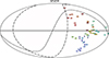 |
Fig. B.1. Dipole directions of the position-dependent power spectrum in the Planck PR4 SEVEM map (Commander results being very similar), for each multipole up to ℓ = 50. The black solid, dashed and dash-dotted lines correspond to the galactic, ecliptic and supergalactic planes, respectively. |
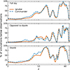 |
Fig. B.2. Comparison between the position-dependent power spectrum in the Planck PR4 CMB temperature data and simulated maps. We average the position-dependent power spectrum over the full sky (upper panel), and the two hemispheres defined by the dipole of each multipole (opposed to dipole in the middle panel and dipole direction otherwise), and compare the observed value to the equivalent from the simulations. We show the percentage of simulations having a lower value than the data. Horizontal black dotted lines indicate the 5% and 95% thresholds. |
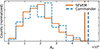 |
Fig. B.3. Distribution of the amplitude of the position-dependent variance dipole (using disks of 4° radius) in the Planck PR4 CMB temperature data illustrating the hemispherical asymmetry anomaly. The orange and blue vertical lines correspond to the observed SEVEM and Commander maps, respectively, and the histograms are obtained from the corresponding 600 SEVEM (orange), and 100 Commander (blue) simulations. None of the simulated CMB maps have a large dipole amplitude value. |
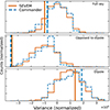 |
Fig. B.4. Same as Fig. 7 but for the position-dependent variance computed with disks of 4° radius as patches. None of the simulated CMB maps have a lower averaged position-dependent variance in the direction opposed to their respective dipoles than the observations (close to the northern supergalactic hemisphere). |
All Tables
Characteristics of the tSZ and kSZ maps constructed from the SLOW, Magneticum and Coruscant hydrodynamical simulations.
All Figures
|
Fig. 1. tSZ (y-Compton) and kSZ signals from the local Universe in the SLOW constrained simulation. The upper panels only include the most local structures (up to 110 Mpc, denoted SLOW-110), and the lower panels use almost the full volume of the box (up to 350 Mpc, denoted SLOW-350). The color scale is logarithmic in the tSZ maps and symmetric logarithmic for the kSZ maps. The main characteristics of these maps are recalled in Table 2. |
| In the text | |
|
Fig. 2. Pseudo-Cℓ of the Planck PR4 CMB temperature maps from SEVEM (top panel) and Commander (bottom panel). The solid red lines are measured from cleaned observed maps, and the dotted black lines are theoretical predictions computed using CAMB. The colored areas are determined from simulations and show their distribution around the median. For the two component separation methods, the observed quadrupole belongs to the lowest 5% of the simulated values (only 15 SEVEM simulations out of 600 have a lower quadrupole, and 4 for Commander). Only 15% of the simulations have a smaller octopole. |
| In the text | |
|
Fig. 3. Lack of correlation on large angular scales (θ > 60°) in the cleaned Planck PR4 CMB temperature maps. We show the distribution of the statistic S1/2 (Eq. (4)) measured in the Planck PR4 simulations, and the vertical lines (on the left) are the observed values. The dashed blue and solid orange lines correspond to the Commander and SEVEM maps, respectively. None of the measured S1/2 in the simulations is as low as in the observations. |
| In the text | |
|
Fig. 4. Quadrupole-octopole alignment in the cleaned Planck PR4 CMB temperature maps. In the upper panel, we show the distribution of SO (see Eq. (6)), indicating the planarity of the octopole is. Higher values are obtained for 59 SEVEM simulations (out of 600) and 9 (out of 100) for Commander. In the lower panel, we show the distribution of SQO, measuring the alignment between quadrupole and octopole. Only one simulation in both sets has a higher SQO value than the observed data. The solid orange and dashed blue lines correspond to the SEVEM and Commander maps, respectively. |
| In the text | |
|
Fig. 5. Quadrupole-octopole alignment in the cleaned Planck PR4 CMB temperature maps. The preferred direction of the quadrupole is given by the orange circle and blue crosses for SEVEM and Commander, respectively. The orange and blue contours, which are almost superimposed, correspond to the areas where S(Ω) (defined in Eq. (6)) is within 3% of its maximum (preferred direction of the octopole), for SEVEM and Commander respectively. The background map is the sum of the SEVEM CMB quadrupole and octopole. The solid and dashed black lines correspond to the galactic and ecliptic planes, respectively. We only show the preferred directions in the northern galactic hemisphere. |
| In the text | |
|
Fig. 6. Preferred direction of the variance asymmetry in the Planck PR4 CMB temperature maps. Dipoles are computed from the position-dependent variance maps computed using HEALPix pixel patches. The data dipole directions are given by the large blue crosses and orange disks for Commander and SEVEM, respectively, and the small markers are for the corresponding simulations. The blue and orange lines are the planes orthogonal to these observed dipoles. The solid, dashed and dash-dotted lines correspond to the galactic, ecliptic and supergalactic planes, respectively. |
| In the text | |
|
Fig. 7. Hemispherical asymmetry in the Planck PR4 CMB temperature data. From left to right, we show the position-dependent variance, skewness, and kurtosis averaged over the full sky (upper row), and the two hemispheres defined by the plane orthogonal to the position-dependent variance of each individual map (opposite and same directions as the dipole in the middle and lower rows, respectively). The vertical orange and blue lines correspond to the observed SEVEM and Commander maps, respectively, and the histograms were obtained from the corresponding 600 SEVEM (orange), and 100 Commander (blue) simulations. There is a lack of variance in the hemisphere opposed to the dipole, where 583 (out of 600) SEVEM and 99 (out of 100) Commander simulations have higher values than the data. |
| In the text | |
|
Fig. 8. Local tSZ (left) and kSZ (right) power spectra compared to the average. The solid red and blue lines are power spectra measured from the maps shown in Fig. 1, constructed by integrating electron gas properties through the SLOW simulation from the position of the Milky Way to rmax = 110 and rmax = 350 Mpc, respectively. The colored areas are 90% percentiles determined from the sets of maps where the center for the integration is displaced in the SLOW simulation, slightly (by 1 Mpc from the Milky Way) in orange (SLOW-near), and strongly (more than 100 Mpc between each center) in green (SLOW-grid). The dashed lines show theoretical predictions computed in the halo model, where the red and blue lines are integrated up to rmax = 110 and rmax = 350 Mpc, and the black lines correspond to the full expected tSZ or kSZ signals. The tSZ power spectrum is shown at the frequency 143 GHz. |
| In the text | |
|
Fig. 9. Same as Fig. 8, where the most prominent cluster in each simulation has been masked by a disk with a radius of 10°. In the local Universe, this corresponds to the Virgo cluster. |
| In the text | |
|
Fig. 10. Same as Fig. 8, where the two most prominent clusters in each simulation have been masked by a disk with a radius of 10°. In the local Universe, this corresponds to the Virgo and Centaurus clusters. |
| In the text | |
|
Fig. 11. tSZ and kSZ power spectra up to rmax = 110 Mpc from several hydrodynamical simulations. As in Fig. 8, the solid red line and the orange and green areas are determined from the SLOW simulation, and the dashed lines are the corresponding predictions from the halo model. The solid purple lines are estimated from local Universe maps determined from the Coruscant simulation, and the gray areas are 90% percentiles from the Magneticum simulation. |
| In the text | |
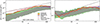 |
Fig. 12. Same as Fig. 11, where the most prominent cluster have been masked in each map. |
| In the text | |
|
Fig. 13. Impact of the local Universe SZ signal on the lack of correlation at angular scales θ > 60°. We measure the difference of S1/2 (see Eq. (4)) between Gaussian CMB realizations with or without the local tSZ (at 143 GHz) and kSZ effects, when the galactic plane alone was masked (in red), and when the galactic plane and Virgo were masked (in green). The distributions are shown for both the full set (solid lines) and for the 5% (dashed) simulations where the lack of correlation is strongest (smallest S1/2). |
| In the text | |
|
Fig. 14. Impact of the local Universe SZ signal on the quadrupole-octopole alignment. We measure the difference of SQO (see Eq. (6)) between Gaussian CMB realizations with or without the local tSZ (at 143 GHz) and kSZ effects, when the galactic plane alone was masked (in red), and when the galactic plane and Virgo were masked (in green). The distributions are shown for both the full set (solid lines) and the 5% (dashed) simulations where the alignment is strongest (largest SQO). |
| In the text | |
|
Fig. 15. Impact of the local Universe SZ signal on the hemispherical asymmetry. We measure the difference of Ad (amplitude of the position-dependent variance dipole; see Sect. 3.3 for details) between Gaussian CMB realizations with or without the local tSZ (at 143 GHz) and kSZ effects, when the galactic plane alone was masked (in red), and when the galactic plane and Virgo were masked (in green). The distributions are shown for both the full set (solid lines) and the 5% (dashed) simulations where the hemispherical asymmetry is strongest (largest Ad). |
| In the text | |
|
Fig. A.1. Maps of the disk, HEALPix pixel and Mexican needlet patches used in this work to evaluate position-dependent statistics. The three complete sets include 3072 4° radius disks, 768 pixels (corresponding to the pixels of a Nside = 8 HEALPix map) and 192 Mexican needlets (p = 1, b = 4 and j = 1). Note that all patches have been set to 1 at their center in this figure. |
| In the text | |
|
Fig. B.1. Dipole directions of the position-dependent power spectrum in the Planck PR4 SEVEM map (Commander results being very similar), for each multipole up to ℓ = 50. The black solid, dashed and dash-dotted lines correspond to the galactic, ecliptic and supergalactic planes, respectively. |
| In the text | |
|
Fig. B.2. Comparison between the position-dependent power spectrum in the Planck PR4 CMB temperature data and simulated maps. We average the position-dependent power spectrum over the full sky (upper panel), and the two hemispheres defined by the dipole of each multipole (opposed to dipole in the middle panel and dipole direction otherwise), and compare the observed value to the equivalent from the simulations. We show the percentage of simulations having a lower value than the data. Horizontal black dotted lines indicate the 5% and 95% thresholds. |
| In the text | |
|
Fig. B.3. Distribution of the amplitude of the position-dependent variance dipole (using disks of 4° radius) in the Planck PR4 CMB temperature data illustrating the hemispherical asymmetry anomaly. The orange and blue vertical lines correspond to the observed SEVEM and Commander maps, respectively, and the histograms are obtained from the corresponding 600 SEVEM (orange), and 100 Commander (blue) simulations. None of the simulated CMB maps have a large dipole amplitude value. |
| In the text | |
|
Fig. B.4. Same as Fig. 7 but for the position-dependent variance computed with disks of 4° radius as patches. None of the simulated CMB maps have a lower averaged position-dependent variance in the direction opposed to their respective dipoles than the observations (close to the northern supergalactic hemisphere). |
| In the text | |
Current usage metrics show cumulative count of Article Views (full-text article views including HTML views, PDF and ePub downloads, according to the available data) and Abstracts Views on Vision4Press platform.
Data correspond to usage on the plateform after 2015. The current usage metrics is available 48-96 hours after online publication and is updated daily on week days.
Initial download of the metrics may take a while.