| Issue |
A&A
Volume 692, December 2024
|
|
|---|---|---|
| Article Number | A146 | |
| Number of page(s) | 23 | |
| Section | Extragalactic astronomy | |
| DOI | https://doi.org/10.1051/0004-6361/202347879 | |
| Published online | 06 December 2024 | |
Does the HCN/CO ratio trace the star-forming fraction of gas?
II. Variations in CO and HCN emissivity
1
Leiden Observatory, Leiden University, PO Box 9513 2300 RA, Leiden, The Netherlands
2
Department of Physics & Astronomy, University of Waterloo, Waterloo, ON N2L 3G1, Canada
3
Waterloo Centre for Astrophysics, University of Waterloo, 200 University Ave W, Waterloo, ON N2L 3G1, Canada
4
Department of Physics & Astronomy, McMaster University, 1280 Main St W, Hamilton, ON L8S 4M1, Canada
5
Argelander-Institut für Astronomie, Universität Bonn, Auf dem Hügel 71, 53121 Bonn, Germany
⋆ Corresponding author; abemis@uwaterloo.ca
Received:
5
September
2023
Accepted:
30
September
2024
We modeled emissivities of the HCN and CO J = 1–0 transitions across a grid of molecular cloud models encapsulating observed properties that span from normal star-forming galaxies to more extreme merging systems. These models are compared with archival observations of the HCN and CO J = 1–0 transitions, in addition to the radio continuum at 93 GHz, for ten nearby galaxies. We combined these model emissivities with the predictions of gravoturbulent models of star formation presented in the first paper in this series. In particular, we explored the impact of excitation and optical depth on CO and HCN emission and assess if the HCN/CO ratio tracks the fraction of gravitationally bound dense gas, fgrav, in molecular clouds. We find that our modeled HCN/CO ratios are consistent with the measurements within our sample, and our modeled HCN and CO emissivities are consistent with the results of observational studies of nearby galaxies and clouds in the Milky Way. CO emission shows a wide range of optical depths across different environments, ranging from optically thick in normal galaxies to moderately optically thin in more extreme systems. HCN appears only moderately optically thick and shows significant subthermal excitation in both normal and extreme galaxies. We find an anticorrelation between HCN/CO and fgrav, which implies that the HCN/CO ratio is not a reliable tracer of fgrav. Instead, this ratio appears to best track gas at moderate densities (n > 103.5 cm−3), which is below the typically assumed dense gas threshold of n > 104.5 cm−3. We also find that variations in CO emissivity depend strongly on optical depth, which is a product of variations in the dynamics of the cloud gas. HCN emissivity is more strongly dependent on excitation, as opposed to optical depth, and thus does not necessarily track variations in CO emissivity. We further conclude that a single line ratio, such as HCN/CO, will not consistently track the fraction of gravitationally bound, star-forming gas if the critical density for star formation varies in molecular clouds. This work highlights important uncertainties that need to be considered when observationally applying an HCN conversion factor in order to estimate the dense (i.e., n > 104.5 cm−3) gas content in nearby galaxies.
Key words: ISM: clouds / ISM: general / ISM: molecules / galaxies: general / galaxies: ISM / galaxies: star formation
© The Authors 2024
 Open Access article, published by EDP Sciences, under the terms of the Creative Commons Attribution License (https://creativecommons.org/licenses/by/4.0), which permits unrestricted use, distribution, and reproduction in any medium, provided the original work is properly cited.
This article is published in open access under the Subscribe to Open model. Subscribe to A&A to support open access publication.
1. Introduction
The HCN/CO ratio is commonly used to assess the fraction of dense gas (≳104–105 cm−3) that might be associated with star formation in external galaxies. The seminal work by Gao & Solomon (2004a,b) found a linear scaling (slope of unity) between the logarithm of the HCN luminosity and the star formation rate as traced in the infrared (IR)1 for a diverse sample of galaxies, including normal disk galaxies as well as more extreme ultra-luminous and luminous infrared galaxies (U/LIRGs). This correlation suggests that HCN is a useful tracer of star-forming gas for a range of galaxy types. The linear scaling between LIR and LHCN also implies that the critical density for HCN J = 1–0 emission, ncrit, HCN, is close to a common mean threshold density, nthresh, that is important for star formation. Although individual galaxies have scatter in the LIR and LHCN relationship, a linear scaling implies that the average value of LIR/LHCN = 900 L⊙ (K km s−s pc2) (Gao & Solomon 2004b) is relatively constant over many orders of magnitude. However, systematic deviations from linearity have since been found in U/LIRGs (Graciá-Carpio et al. 2008; García-Burillo et al. 2012), at subkiloparsec scales in disk galaxies (Usero et al. 2015; Chen et al. 2015; Gallagher et al. 2018a; Querejeta et al. 2019; Jiménez-Donaire et al. 2019; Bešlić et al. 2021; Neumann et al. 2023), and at subkiloparsec scales in galaxy mergers (Bigiel et al. 2015; Bemis & Wilson 2019). These nonlinearities do not appear associated with the presence of an active galactic nucleus (AGN), which otherwise could enhance HCN emissivity via infrared pumping (Sakamoto et al. 2010). In the absence of an AGN, these variations in emissivity can be interpreted as a fundamental difference in the depletion time of dense gas within different systems, which may signal a connection between star formation and environment within galaxies.
Variations are also seen in the star formation efficiency of dense gas in our own Milky Way. Gas in the central molecular zone (CMZ) of the Milky Way is dense (n ∼ 104 cm−3) and warm (T ∼ 65 K) compared to gas in the disk (n ∼ 102 cm−3, T ∼ 10 K, Rathborne et al. 2014; Ginsburg et al. 2016). Despite their abundance of dense gas (Mills 2017), some clouds in the CMZ display a lack of star formation (Longmore et al. 2013; Kruijssen et al. 2014; Walker et al. 2018). CMZ clouds experience high external pressures (∼108 K cm−3), and it is theorized that their lack of star-forming activity may be due to a higher star formation threshold density as a result of higher internal turbulent pressures (Walker et al. 2018). Additionally, shear from solenoidal turbulence may also suppress the onset of star formation in the CMZ (Federrath et al. 2016). A lack of star formation in dense gas traced by HCN is also apparent in the centers of nearby disk galaxies (Gallagher et al. 2018a; Querejeta et al. 2019; Jiménez-Donaire et al. 2019; Bešlić et al. 2021; Neumann et al. 2023) and the nuclei of the Antennae galaxies (NGC 4038/9, Bemis & Wilson 2019). Gas density is well-constrained in the CMZ, suggesting that there are true variations in star formation from dense gas in this environment relative to the Milky Way disk. Many studies of external galaxies rely on a single molecular gas tracer, HCN, to estimate the dense gas fraction, and recent work calls into question its ability to consistently trace dense gas in molecular clouds (e.g., Kauffmann et al. 2017; Pety et al. 2017; Shimajiri et al. 2017; Barnes et al. 2020; Tafalla et al. 2021, 2023; Santa-Maria et al. 2023). Furthermore, if the star formation threshold density also varies with the local environment within galaxies, a gas fraction estimate from a single line ratio may not reliably track the fraction of gas above this threshold (Bemis & Wilson 2023; Neumann et al. 2023).
In Bemis & Wilson (2023, hereafter Paper I), we assess the ability of the relative intensity of HCN to CO, IHCN/ICO, to determine the fraction of gravitationally bound gas by comparing the observed star formation properties and HCN/CO ratios in ten galaxies to the predictions of analytical models of star formation (Krumholz & McKee 2005; Federrath & Klessen 2012; Hennebelle & Chabrier 2011; Burkhart 2018). In Paper I we find that the trends observed in our sample of dense gas traced by IHCN, the SFR traced by the radio continuum at 93 GHz, and the total molecular gas traced by ICO are best reproduced by gravoturbulent models of star formation with varying star formation thresholds under the assumption that IHCN/ICO is tracing the fraction of gas above a relatively fixed density, such as n ≳ 104.5 cm−3, but not necessarily the fraction of gas that is gravitationally bound or star-forming. Furthermore, in Paper I we show that turbulent models of star formation with varying star formation thresholds predict an increase in the depletion time of dense gas at n ≳ 104.5 cm−3 in clouds with higher dense gas fractions due to higher levels of turbulence. This corroborates observations in the CMZ where star formation appears suppressed relative to the amount of dense gas mass, estimates of turbulent pressure (Pturb) appear higher, and the dominant mode of turbulence may be more solenoidal compared to spiral arms (Federrath et al. 2016; Walker et al. 2018). Similar trends are observed in galaxy centers (Gallagher et al. 2018a; Querejeta et al. 2019; Jiménez-Donaire et al. 2019; Bešlić et al. 2021) and in the nuclei of the Antennae Paper I, although estimates of the dominant turbulent mode are unavailable for these studies.
One key uncertainty in these results is the ratio of the emissivities of HCN and CO (i.e., the conversion of HCN or CO intensity to gas column density) and whether systematic variations in HCN and CO emissivity can occur in such a way that may also contribute to the observed trends. The CO conversion factor, αCO, is estimated to vary with excitation (e.g., Narayanan et al. 2012; Narayanan & Krumholz 2014) and metallicity (e.g., Schruba et al. 2012; Hu et al. 2022a); can be nearly five times lower in U/LIRGs (e.g., Downes et al. 1993); and is lower in the centers of disk galaxies (e.g., Sandstrom et al. 2013). The HCN conversion factor, αHCN, is also likely to vary across different systems (Usero et al. 2015), but may not necessarily track αCO (Onus et al. 2018). Observations of HCN and H13CN in galaxy centers suggest that HCN is only moderately optically thick (Jiménez-Donaire et al. 2017), unlike CO which typically has τCO > 10. The original estimate of αHCN was made under the assumption of optically thick emission (Gao & Solomon 2004a,b). Since HCN emission appears only moderately optically thick, variations in the optical depth of HCN emission could impact the accuracy of gas masses using this estimate of the HCN conversion factor. Thus, the HCN/CO intensity ratio may not scale linearly with the fraction of gas ≳104 cm−3, due to variations in excitation and optical depth. As we refine our understanding of star formation in galaxies, it is clear that we must also adopt a more sophisticated approach to estimating masses using molecular line emission, and we must develop a better understanding of the information that these measurements can provide on star formation.
In this paper we model emissivities of HCN and CO using the non-LTE radiative transfer code RADEX (van der Tak et al. 2007; Leroy et al. 2017a) across a grid of cloud models that encapsulates observed trends in cloud properties that span from from normal star-forming galaxies to U/LIRGs (Sun et al. 2020; Brunetti et al. 2021, 2024). We assess the impact of variations in optical depth and excitation on the emissivities of HCN and CO across this grid, and we compare our modeling results with the star-forming trends observed in the sample of ten galaxies from Paper I using archival ALMA data of the HCN and CO J = 1 → 0 transitions and the radio continuum at 93 GHz (see Wilson et al. 2023 for details on imaging). This sample includes the dense centers of five disk galaxies and five U/LIRGs (see Table 1 of Paper I). In Sect. 2 we describe the model framework that we adopted to derive emissivities using analytical models of star formation, as well as the parameter space we considered. We present the results of our models and compare these results with observations in Sect. 3. Finally, in Sect. 4 we provide a brief discussion and summary of our main results. Throughout the text we take “HCN/CO ratio” to mean the ratio of HCN to CO intensities, unless explicitly stated otherwise.
2. Model framework
We model molecular line emissivities using the radiative transfer code RADEX (van der Tak et al. 2007), and we connect these emissivities to gravoturbulent models of star formation. We present several gravoturbulent models of star formation in Paper I, which predict clouds have gas density distributions that are either purely lognormal (LN, cf. Padoan & Nordlund 2011; Krumholz & McKee 2005; Federrath & Klessen 2012) or a composite lognormal and power-law distribution (LN+PL, cf. Burkhart et al. 2017). We refer to these distributions as the gas density probability density functions (PDFs) for the remainder of the text. We focus on the results of the composite LN+PL models in this analysis.
2.1. Emissivity
We adopt the following definition of the emissivity of a molecular transition (e.g., Leroy et al. 2017a):
Here Imol is the total line intensity of a molecular transition (in units of K km s−1), N is the column density of gas that emits I, Nmol is the molecular column density of an observed molecule (both in units of cm−2), and xmol is the fractional abundance of the molecule relative to the molecular hydrogen, H2. The ratio of the HCN and CO emissivities is then given by
Emissivity is analogous to the inverse of molecular conversion factors (αmol = Xmol/6.3 × 1019, Leroy et al. 2017b), which are commonly used to estimate the mass traced by a molecular transition. In practice, the relationship between the total emissivity of an observed molecular cloud and an appropriate conversion factor also depends on the beam filling fraction and the uniformity of gas properties within the beam (cf. Bolatto et al. 2013).
2.2. Cloud models
Under the assumption that we can derive information of the gas density distribution from estimates of gas velocity dispersion, we build our cloud models using gas density distributions predicted by gravoturbulent models of star formation that employ the gas density variance – mach number relation (cf. Eq. (3)). There are well-established theories connecting the gas density variance (σn/n02) in molecular clouds to mach number (cf. Passot & Vázquez-Semadeni 1998; Beetz et al. 2008; Burkhart et al. 2010; Padoan & Nordlund 2011; Price et al. 2011; Konstandin et al. 2012; Molina et al. 2012; Federrath & Banerjee 2015; Nolan et al. 2015; Pan et al. 2016; Squire & Hopkins 2017; Beattie et al. 2021). In general, these theories predict that the gas density variance increases with mach number, such that (cf. Federrath et al. 2008, 2010; Molina et al. 2012)
where b is the turbulent forcing parameter which describes the dominant mode(s) of turbulence (i.e., compressive, mixed, or solenoidal) and spans b = 1/3 − 1 (Federrath et al. 2008, 2010), ℳ is the sonic mach number, and β is the ratio of thermal to magnetic pressure (cf. Molina et al. 2012). Numerical work shows that a connection is also expected between the 2D gas density variance, σΣ/Σ0, an observable, and mach number (e.g., Brunt et al. 2010a,b; Burkhart & Lazarian 2012). Thus, resolved studies of the gas column density distribution can, in theory, provide information on the Mach number of the initial turbulent velocity field shaping the dynamics of a cloud. Alternatively, lower-resolution studies that are limited to global cloud measurements (as is often the case in extragalactic studies) may also be able to derive information on the gas density distribution using estimates of the gas velocity dispersion. We use this as a basis to build our cloud models and our model parameter space, described in detail in Sect. 2.3. We also highlight the relevant uncertainties for this approach, both in this section and in Appendix A.
We note that there are a number of analytical prescriptions describing the gas density distribution (e.g., Krumholz & McKee 2005; Padoan & Nordlund 2011; Hennebelle & Chabrier 2011; Hopkins 2013; Burkhart 2018). For simplicity, we focus on the piecewise lognormal and power-law distribution from Burkhart (2018) and we note that we do not expect significant changes to our main conclusions if we were to adopt a different prescription. In particular, our models produce gas density distributions with widths and density ranges comparable to those observed in resolved studies of clouds in the Milky Way (cf. Schneider et al. 2022). The piecewise volume density PDF is given in Paper I (Eq. (16)) and is originally given in Burkhart (2018) (Eqs. (2) and (6)) in terms of the logarithmic density, s = ln(n/n0), where n is gas volume density and n0 is the mean gas volume density. We refer to Paper I and Burkhart (2018) for a thorough description of these models in terms of the logarithmic density. Here we briefly summarise the main components of these models in terms of the linear gas volume density, n, which is directly used in our modeling of molecular line emissivities.
Each cloud model is comprised of a piecewise lognormal and power-law gas volume density PDF (n–PDF). The lognormal component of the n–PDF has a characteristic gas density variance, σn/n02 and mean density, n0. We note that the logarithmic gas density PDF (Eq. (16) in Paper I) can be converted to its linear form via ps = n pn. Likewise, the logarithmic variance (Eq. (17) in Paper I), σs2, can be converted to its linear form using σn/n02 = exp(σs2) − 1 (cf. Federrath et al. 2008). The power-law component of the n–PDF is primarily characterized by its slope, αPL, and the power-law slope of pn is related to the slope of ps via αPL(n) = αPL(s)−1. The two components of the n–PDF are analytically connected such that they are smoothly varying (Burkhart 2018). Similar to Paper I, we fix b = 0.4, which represents stochastic mixing between the two turbulent forcing modes (Federrath et al. 2010), and we neglect magnetic fields and take β → ∞. We illustrate example n–PDFs in Fig. 1 that are sampled from our model parameter space, described in Sect. 2.3.
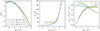 |
Fig. 1. Three models that are representative of clouds in (1) the PHANGS sample (NGC 2903), (2) NGC 4038/9, and (3) NGC 3256. Left: Example n–PDFs from our model parameter space assuming αPL = 3. Center: Temperature profiles of the example models. Right: Emissivity profiles of the example models. CO emissivity is shown as solid lines, and HCN emissivity is shown as dashed lines. The mass-weighted emissivity, ⟨ϵmol⟩, is given by Eq. (11). The range of densities over which radiative transfer is applied is slightly different between models, and depends on the average gas surface density of the model (see Sect. 2.3). We plot pn over a wider range of volume densities (left plot) than those used when performing radiative transfer (center and right plots). |
2.3. The model parameter space
We constructed our model parameter space to capture observed trends in cloud properties associated with star-forming molecular gas clouds. As described in Sect. 2.2, each unique model is described by its variance, σn/n0, mean density, n0, and power-law slope, αPL. Within σn/n0 is a dependence on the turbulent gas velocity dispersion, σv, and gas kinetic temperature, Tkin, via the sonic mach number,  (assuming isotropy), where σv is the 1D turbulent velocity dispersion,
  is the gas sound speed, k is the Boltzmann constant, μ is the mean molecular weight of the gas, and mH is the mass of a Hydrogen atom. We assume a mean molecular weight of μ = 2.33 (e.g., Kauffmann et al. 2008). Each individual model is therefore defined by a unique set of n0, σv, Tkin, and αPL. We discuss how we set each of these parameters below.
2.3.1. Turbulent gas velocity dispersion, σv:
In Paper I, we selected a model parameter space such that the median Σmol − σv trend generally follows the Σmol − σv fit to PHANGS (Physics at High Angular resolution in Nearby GalaxieS, Leroy et al. 2021) data in Sun et al. (2018) and Milky Way cloud-scale studies (Heyer et al. 2009; Field et al. 2011). In this paper, we used cloud-scale (R = 40–45 pc) measurements of cloud properties derived from observations of the CO J = 2–1 line from the PHANGS sample (Sun et al. 2020), NGC 3256 (Brunetti et al. 2021) and the Antennae (Brunetti et al. 2024) as the basis of our model parameter space. We randomly sampled measurements from each of these cloud-scale studies, that include pairs of molecular gas surface density and velocity dispersion, Σmol and σv. Constructing our model parameter space this way ensures that our models include representatives of cloud-scale observations of normal galaxies (from PHANGS), as well as more extreme systems that are representative of merging galaxies in our study (i.e., NGC 3256 and the Antennae). The Antennae and NGC 3256 are both in our lower-resolution sample from Paper I and this paper. We plot the corresponding cloud coefficients (σv2/R vs. Σmol, where R is the size of the molecular component of the cloud, Heyer & Dame 2015; Field et al. 2011) of our model parameter space in comparison to those from the PHANGS sample (Sun et al. 2020) and those from our lower-resolution study (∼50–900 pc, see Table 1 in Paper I) in Fig. 2.
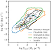 |
Fig. 2. The model parameter space showing the range of gas velocity dispersions and gas surface densities considered in our analysis. The model points are plotted as gray points in the σv2/R − Σmol parameter space, and include a mix of cloud measurements from the PHANGS sample (Sun et al. 2020), NGC 4038/9 (Brunetti et al. 2024), and NGC 3256 (Brunetti et al. 2021). We also outline σv2/R − Σmol measurements of the Sun et al. (2020) PHANGS galaxies at 90 pc resolution (R = 45 pc, blue contours), NGC 4038/9 at 80 pc resolution (R = 40 pc, orange contours), and NGC 3256 at 80 pc resolution (R = 40 pc, green contours). The lower resolution data from Paper I are outlined by the black solid line. Example models from Fig. 1 are indicated in this plot as the blue (1), orange (2), and green (3) points. |
Setting our model parameter space this way relies on the assumption that the CO velocity dispersion tracks the turbulent velocity dispersion at these scales. In Appendix A, we discuss in detail the uncertainties and evidence for use of observational estimates of gas velocity dispersion from molecular line emission, and summarize the main points here. Using simulations, Szűcs et al. (2016) find the measured 12CO velocity dispersion is within ∼30–40% of the turbulent 1D velocity dispersion in their cloud simulations, on average, and argue that the CO velocity dispersion should trace the turbulent velocity dispersion. This is smaller than the expected uncertainty on the mass conversion factor (Szűcs et al. 2016; Bolatto et al. 2013), which is up to a factor of two. Additionally, a weak correlation is observed between mach number estimated from various molecular line transitions and gas density variance in resolved clouds in the Milky Way (e.g., Padoan et al. 1997; Brunt 2010; Ginsburg et al. 2013; Kainulainen & Tan 2013; Federrath et al. 2016; Menon et al. 2021; Marchal & Miville-Deschênes 2021; Sharda & Krumholz 2022), although there is significant scatter potentially due to uncertainties in b (Kainulainen & Federrath 2017).
We cannot exclude the possibility of large-scale motions impacting the measured velocity dispersions of studies at 45–50 pc. For example, Federrath et al. (2016) used HNCO to estimate turbulent velocity dispersion in G0.253+0.016 (The Brick) and subtracted a large-scale gradient that appears to contribute ∼40–50% of the measured velocity dispersion, possibly from shear due to its location in the CMZ of the Milky Way. Using the velocity profiles derived from Lang et al. (2020), we conclude that a small fraction of clouds in the PHANGS sample will be impacted by shear motions towards the centres of these disk galaxies (with contributions > 50% to the measured velocity dispersion). It is more difficult to quantify the large-scale motions of gas within the mergers NGC 3256 and NGC 4038/9. Gas streaming motions or shear may bias measured velocity dispersions towards larger values (Sun et al. 2020; Henshaw et al. 2016; Federrath et al. 2016). In general, the measured velocity dispersions are larger in the mergers; however, the gas density PDF is also expected to be wider in mergers (with more dense gas) due to enhanced compressive turbulence (cf. Renaud et al. 2014). Thus, we conclude that the velocity dispersion measurements from CO likely track the turbulent velocity dispersion, and quote a typical uncertainty of 50%.
Finally, we note that clouds in the PHANGS sample and in NGC 3256 are marginally resolved at 40–45 pc scales (cf. Rosolowsky et al. 2021; Brunetti & Wilson 2022), and we expect the Antennae to have cloud sizes intermediate between those found in the PHANGS galaxies and NGC 3256. For comparison, a typical size of clouds in the Milky Way is 30 pc, with a large range from < 1 pc to 100 pc (Miville-Deschênes et al. 2017). Thus, there will be some variation in how resolved each cloud is in the three studies we take measurements from (Sun et al. 2020; Brunetti et al. 2021, 2024). However, we do not expect molecular velocity dispersions in the galaxies to be significantly impacted by observational effects such as beam smearing, since the systems studied are relatively face on (Sun et al. 2020; Brunetti et al. 2021, 2024). Additionally, the gas density variance – mach number relation (cf. Eq. (3)) will hold on scales smaller than the cloud size, since turbulence is expected to produce self-similar structure (e.g., Elmegreen & Scalo 2004; Dib et al. 2008; Burkhart et al. 2013).
2.3.2. Mean gas density, n0:
We derived a mean gas density, n0, based on the molecular gas surface density estimates, Σmol. We estimated a minimum mean gas density by converting Σmol to a volume density assuming a spherical geometry (n(R), where R is the assumed size of the molecular cloud that is set by the pixel size), such that n0 = Σ/R. We note that we also considered different prescriptions for calculating mean gas density based on the assumption of energy equipartition (i.e., fixed virial parameter) and dynamical equilibrium in a gas disk (Wilson et al. 2019). We find similar results regardless of the prescription we choose for n0 and therefore only present the results assuming n0 = Σ/R2. We also acknowledge that the Σmol measurements from these cloud scale studies are still prone to uncertainties in the CO conversion factor. However, we confirm that our modeled CO J = 1–0 intensities with ICO are consistent with the intensities measured in our lower resolution sample (see Fig. 3), with only small offsets.
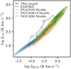 |
Fig. 3. Modeled ICO and IHCN compared with the measured intensities of the Paper I sample (solid contours) and the EMPIRE sample (dashed contours Jiménez-Donaire et al. 2019). The blue filled contours are models whose Σ and σv are taken from the PHANGS sample (Sun et al. 2020), the orange filled contours are those taken from NGC 4038/9 (Brunetti et al. 2024), and the green filled contours are those taken from NGC 3256 (Brunetti et al. 2021). Ten contours are drawn in even steps from the 16–100th percentile. |
2.3.3. Power-law slope of the n–PDF, αPL:
We aim to capture observed star formation scaling relations in our study, in addition to capturing observed cloud properties. Following Paper I, we use the gravoturbulent models of star formation from Burkhart (2018) and Burkhart & Mocz (2019), which assume the n–PDF is a combination of a lognormal turbulence-dominated component and gravity-dominated power-law tail at high densities. We use these models to estimate ϵff = tdep/tff (star formation efficiency per free-fall time), tdep, and ΣSFR (the star formation rate surface density). Table 2 in Paper I describes how each of these quantities are derived. In this framework, the choice of αPL (the slope of the power-law component of the n–PDF in the gravoturbulent star formation models of Burkhart 2018; Burkhart & Mocz 2019) has an impact on the resulting ϵff such that steeper αPL values result in higher ϵff and vice versa. We choose αPL = 3 as our fiducial value (which corresponds to k = 1.5, see Eq. (8))3. Similar to Paper I, we must also assume a local efficiency of ϵ0 so that values of tdep and ΣSFR derived from our models are consistent with observations. ϵ0 accounts for a reduction in star formation efficiency from stellar feedback processes. For αPL = 3 we take ϵ0 = 0.01, which returns ϵff ≈ 0.01–0.1, and is consistent with expectations from observations and simulations (e.g., Salim et al. 2015; Utomo et al. 2018; Sharda et al. 2018; Hu et al. 2022b).
2.3.4. Gas kinetic temperature, Tkin:
We estimated Tkin following the prescription in Sharda & Krumholz (2022), which assumes thermal equilibrium balance of heating and cooling processes in the presence of protostellar radiation feedback:

This equation includes compressional heating (Γc), cosmic ray heating (ΓCR), H2 formation heating (ΓH2), metal line cooling (ΛM), H2 cooling (ΛH2), and hydrogen deuteride cooling (ΛHD), as well as the dust-gas energy exchange (Ψgd), which can serve as either a cooling or heating process. The Sharda & Krumholz (2022) prescription includes feedback from active star formation in a semi-analytical framework. In addition to aforementioned cooling and heating mechanisms, Sharda & Krumholz (2022) consider the impact of radiation feedback from existing protostars in the cloud via the dust-gas energy exchange term, where the dust temperature is set by radiation feedback from active star formation. This prescription is adopted from Chakrabarti & McKee (2005) where the authors developed a framework to treat dust temperatures in the presence of a central radiating source (see also, Krumholz 2011).
We adopted the prescription for cosmic ray heating from Krumholz et al. (2023) that is based on the gas depletion time. Krumholz et al. (2023) estimate the average cosmic ray ionization rate, ζCR, to be
The comic ray heating rate is then
where we have taken the average energy per ionization to be qCR = 12.25 eV, which is appropriate for molecular gas (Wolfire et al. 2010). We use tdep estimates that are consistent with the molecular gas star formation laws found by Bigiel et al. (2008) and Wilson et al. (2019). The original prescription used by Sharda & Krumholz (2022) from Crocker et al. (2021) overestimates the gas temperature for molecular clouds.
In addition to these processes included in Sharda & Krumholz (2022), we also incorporated mechanical heating,
which is potentially important for more turbulent clouds (Pan & Padoan 2009; Ao et al. 2013), such as those in mergers or at the centers of barred galaxies. We find that on average over the cloud model, turbulent heating dominates in the models using NGC 4038/9 and NGC 3256 gas surface density and velocity dispersion measurements, while cosmic ray heating dominates in the models using gas surface density and velocity dispersion measurements from PHANGS galaxies. We show example temperature profiles for average PHANGS, NGC 4038/9, and NGC 3256 models in Fig. 1. For low density regions near the exterior of the model clouds, the heating/cooling model sometimes produces temperature increases, which are likely unphysical. At these low densities we fix the temperature to the minimum value over the model cloud (Fig. 1). We note that we assume a solar metallicity composition of the gas for all our cloud models for simplicity, ignoring the metallicity dependence of Tkin.
2.4. Applying radiative transfer
We used RADEX (van der Tak et al. 2007) to perform radiative transfer and calculate emissivities of our cloud models. Each cloud model is comprised of an n−PDF distribution with 500 resolution elements across the PDF in volume density. We run RADEX at each resolution element across the n−PDF, using the escape probability formulation and adopting its default uniform sphere geometry. For each resolution element in our cloud model, RADEX computes a line flux, optical depth, and excitation temperature that we later use to calculate PDF-averaged properties of each cloud model (see Sect. 2.5). To perform its radiative transfer calculation, RADEX requires the input of H2 volume density, molecular column density, gas kinetic temperature, and molecular line width at each resolution element. In Sect. 2.3 we describe how we set fiducial values of mean gas density, n0, velocity dispersion σv, and kinetic temperature, Tkin for each individual model across our model parameter space. We describe how these physical inputs translate to the range of volume and column densities required for each model in the paragraphs below.
To provide RADEX with a molecular column density for each volume density in the model, we assumed a power-law density distribution for the radial H2 volume (n) and column (N) density distributions. One zone models bypass this requirement by assuming a fixed optical depth (e.g., Leroy et al. 2017b), which indirectly determines the n − N relationship, but can underestimate molecular abundances at high densities, and overestimate them at low densities. We therefore adopt power-law radial density distributions that are more realistic for molecular clouds. Spatial density gradients are observed in real molecular clouds, and the slopes of spatial density gradients are potentially connected to the shape of their n–PDF (cf. Federrath & Klessen 2013). Furthermore, these slopes are likely connected to the star formation properties of molecular clouds (Tan et al. 2006; Elmegreen 2011; Parmentier 2014; Kainulainen et al. 2014; Parmentier 2019). The Burkhart (2018) and Burkhart & Mocz (2019) models predict a connection between the power-law slope of the n–PDF and ϵff, and this behaviour has also been observed in Milky Way clouds (Federrath & Klessen 2013). We therefore used the power-law slope of the n–PDF of our models, αPL, to determine the gas density gradient of our models.
Federrath & Klessen (2013) show that the slope of the gradient in a radially symmetric density distribution will be related to the slope of the corresponding n−PDF if they both follow power-law scalings. Using this scaling for spherical geometries in Federrath & Klessen (2013), we connect the slope of the high-density power-law tail of the n−PDF (αPL) to the radial slope of the clump density profile, k, via (cf. Federrath & Klessen 2013):

For comparison, a power-law with k = 2 is consistent with the expectation for isothermal cores (Shu 1977), and results in an n−PDF slope of αPL = 2.5. Shallower n−PDF slopes then correspond to steeper spatial density gradients and vice versa.
The radially symmetric approximation assumed above is only analytically exact for the gravitationally bound gas in the power-law tail of the n−PDF. The gas outside of the power-law tail is primarily governed by turbulence, which produces fractal, self-similar structure (e.g., Elmegreen & Falgarone 1996; Schneider et al. 2011). Self-similarity implies there is no characteristic scale of the gas, but this is not inconsistent with the existence of density gradients in turbulent gas. In the interest of simplicity we also adopt the same power-law density gradient for the gas that we attribute to the lognormal component of the n−PDF. We implement this by adopting a power law for the radial volume and column density distributions, normalised to surface values (see Eqs. (9) and (10), respectively.) The radial volume density distribution is then given by
where r is the radial coordinate, R is the size of the molecular component of the cloud, and n(R) is the volume density of the molecular cloud. We assumes that, in general, the radial profile of the column density will track the radial profile of the volume density. This general trend is consistent with the assumption of either a stiff equation of state (temperature increases with density) or an isothermal equation of state (Federrath & Banerjee 2015). The gas-temperature relationship in our models is, on average, consistent with a stiff equation of state. Since the exact trend varies from model to model, we simply adopt
where N(R) is the column density at the surface of the molecular cloud and is consistent with an isothermal cloud following and ideal gas equation of state. We then derived molecular column density distributions by multiplying the radial H2 column density distribution (Eq. (10)) by the appropriate absolute molecular abundance. Although abundance variations are possible within our sources, we present the results of our models assuming fixed molecular abundances xHCN = 10−8 and xCO = 1.4 × 10⁻⁴ relative to H2 when converting N to a molecular column density (i.e., NHCN or NCO) (Draine 2011). We show example emissivity profiles for several models in Fig. 1. We note that we assumed fixed abundances so that the results of our modeling focus on the impact of variations in turbulent velocity dispersion on HCN and CO emissivities. We run additional models to assess the impact of varying the absolute abundance of HCN and CO on model output, and we present these results in Appendix B. In summary, we find that variations in molecular abundance have a moderate impact on the optical depths of HCN and CO emission, but that these variations do not significantly impact the various correlations between HCN, CO, and molecular cloud properties considered in this work.
2.5. Deriving emissivity and intensity from molecular cloud models
Using the framework described in Sects. 2.1–2.4, we numerically solved for CO and HCN J = 1–0 emissivities. Similar to Leroy et al. (2017b), we weighted the unintegrated emissivities (Eq. 1) by the mass distribution of model clouds, pn, and integrate to determine the mass-weighted emissivity,
where we have re-written Eq. (1) in terms of n and “mol” denotes HCN or CO. When calculating ⟨ϵmol⟩, we numerically integrated the PDF over densities that are relevant to molecular gas, roughly ∼10–108 cm−3. This produces a mass-averaged molecular line emissivity with units of K km s−1 cm2. As Leroy et al. (2017b) point out, 1/⟨ϵmol⟩ can be recast in units of M⊙/pc2 [K km s−1]−1, similar to a molecular line luminosity-to-mass conversion factor. We note that in this work we primarily model quantities that are surface densities (i.e., molecular intensity and column density). However, we are still able to compare the relative mass conversion factors of HCN and CO using properties of the n–PDF, and we explore the difference between emissivity and conversion factors more in Sect. 3.2.
Similar to Eq. (1), the modeled emissivity can be parameterized by an average intensity, ⟨Imol⟩, and an average H2 column density, ⟨NH2, mol⟩, over which the molecular transition is sensitive to: ⟨ϵmol⟩=⟨Imol⟩/⟨NH2, mol⟩. Thus, if we know ⟨NH2, mol⟩, we can derive intensities that are analogous to what are measured in observations of individual molecular clouds. We estimated the average column of mass that a transition is sensitive to, ⟨NH2, mol⟩, from our models using
where N(n) is the H2 column density corresponding to H2 volume density n, and the two quantities are related via Eqs. (9) and (10) in our models. Using ⟨NH2, mol⟩, we derived intensities from our emissivities that can be compared with those measured in our sample from Paper I and the EMPIRE sample (Jiménez-Donaire et al. 2019).
RADEX also returns optical depth and excitation temperature for a given molecular transition at each n across the n–PDF. We determined a fiducial optical depth, ⟨τmol⟩, and excitation temperature, ⟨Tex, mol⟩, for a given molecular transition of each cloud model by calculating the expectation values of these quantities weighted by emissivity via
These estimates of ⟨τmol⟩ and ⟨Tex, mol⟩ are useful for comparison to observations.
3. Model results
We present the model results in the following sections in Figs. 3– 10. In Sect. 3.1 we discuss the impact of excitation and optical depth on the modeled CO and HCN intensities and illustrate these results using the first set of plots (Figs. 3–5). We constrain the characteristic gas densities that the HCN/CO ratio is sensitive to in Sect. 3.2 (cf. Fig. 6). We explore trends in the CO and HCN emissivity (⟨ϵCO⟩ and ⟨ϵHCN⟩) and luminosity-to-mass conversion factors (αCO and αHCN, cf. Fig. 7) in Sect. 3.3. In Sects. 3.4 and 3.5, we explore if the IHCN/ICO ratio traces the fraction of gravitationally bound gas (Sect. 3.4), as well as how variations in CO and HCN emissivity impact our interpretation of star formation scaling relations (Sect. 3.5). We note that we sometimes differentiate between models that represent clouds from different star-forming regimes (i.e., PHANGS-type vs. NGC 3256-type and NGC 4038/9-type) and color the results presented in some figures accordingly.
In Sects. 3.2, 3.4, and 3.5, we combine the predictions of the LN+PL analytical models of star formation (Burkhart 2018) with the results of our radiative transfer modeling. For convenience, we produce a summary of the most relevant equations in the bottom of Table 2 in Paper I describing how various quantities are calculated. In these sections we explore how variations in CO and HCN emissivity, as well as variations in the CO and HCN luminosity-to-mass conversion factors, may impact observed star formation scaling relations. We mimic the results of observational studies by applying common conversion factors to our modeled molecular line intensities to derive gas surface densities (method one), and we compare these results with the true model predictions (method two). For method one, the modeled molecular intensities are multiplied by constant conversion factors, as we have done with our sample from Paper I and the EMPIRE sample. We choose a value that is intermediate between the Milky Way and starburst values for αCO: αCO = 3 [M⊙ (K km s−1 pc2)−1] and αHCN = 3.2 αCO to produce estimates of gas mass surface densities, which are the same values used in Paper I.
3.1. Excitation and optical depth
We show the modeled CO and HCN intensities compared to the intensities measured in our sample from Paper I and the EMPIRE sample from Jiménez-Donaire et al. (2019) in Fig. 3. The ranges of HCN and CO J = 1–0 intensities produced by our models encompass those we measure in the disk galaxies of the EMPIRE sample (IHCN = 0.4–20.5 K km s−1 and ICO = 21.6–331.5 K km s−1, Jiménez-Donaire et al. 2019) and our more extreme sample of galaxies including U/LIRGs and galaxy centers (IHCN = 0.8–814.5 K km s−1 and ICO = 53.8–2397.4 K km s−1, Bemis & Wilson 2023, cf. Fig. 3). The scatter is less well-matched to observations, which may be due to uncertainties in the relative filling fractions of HCN and CO. We calculate the median absolute deviations (MAD) of our measured and modeled HCN and CO intensities and multiply by 1.4826 to get an estimate of the scatter (standard deviation) that is less sensitive to outliers. We find scatters of σHCN = 1.9 K km s−1 and σCO = 27.2 K km s−1 for the EMPIRE sample, σHCN = 13.2 K km s−1 and σCO = 176.2 K km s−1 for our sample, and σHCN = 3.2 K km s−1 and σCO = 51.2 K km s−1 for all models. We find scatters of HCN and CO intensity for just the PHANGS-type models to be σHCN = 1.2 K km s−1 and σCO = 25.0 K km s−1, which is well-matched to the observations of the EMPIRE sample. In contrast to this, we find σHCN = 64.0 K km s−1 and σCO = 500.0 K km s−1 for the NGC 4038/9 and NGC 3256 models combined. This scatter is less well-matched to our data, although roughly on the same order of magnitude as what is measured in our sample. We discuss the impact of emissivity on the scatter of observations in Sect. 3.5.
Figure 4 presents the modeled CO and HCN J = 1–0 intensities as a function of the excitation temperature and optical depth. We find that the CO J = 1–0 transition is close to LTE for the majority of our models when compared to our estimates of ⟨Tkin⟩. A subset of PHANGS models show slightly subthermal emission, which is due to the average density of these models being below the critical density for CO J = 1–0 (i.e., ∼102 − 3 cm−3), the density at which the majority of CO emission becomes thermalised. The CO J = 1–0 transition is, on average, optically thick for the PHANGS-type models. Towards higher ICO where the models are dominated by NGC 4038/9- and NGC 3256-type clouds, the CO optical depth drops and approaches τ ∼ 1 towards the models with the brightest CO emission. This behavior is similar to the results of previous studies of CO excitation (e.g., Narayanan & Krumholz 2014), where the optical depth of the J = 1–0 transition appears to drop towards gas where CO is more excited (and ΣSFR is high). This is due to the fact that the optical depth of CO J = 1–0 is inversely proportional to velocity dispersion, and that velocity dispersion tends to increase with ΣSFR.
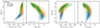 |
Fig. 4. Correlations between modeled ICO (left two plots) and IHCN (right two plots) and their respective excitation temperatures and optical depths determined using Eqs. (13) and (14). The formatting is the same as in Fig. 3. We find that CO optical depth decreases with increasing ICO and CO excitation, in general agreement with the findings of previous studies (e.g., Bolatto et al. 2013; Narayanan et al. 2012; Narayanan & Krumholz 2014). In our models, HCN appears subthermally excited and moderately optically thick, also in agreement with the findings of previous studies (e.g., Dame & Lada 2023; Jiménez-Donaire et al. 2017). |
The HCN J = 1–0 transition appears subthermally excited, which agrees with a number of studies that assess the excitation of HCN in the Milky Way and nearby galaxies (e.g., Dame & Lada 2023; García-Rodríguez et al. 2023; Tafalla et al. 2023). The HCN optical depth is found to be only moderately optically thick for the PHANGS-type clouds in our models, and is in agreement with previous studies towards the centers of disk galaxies (Jiménez-Donaire et al. 2017). These results suggest that variations in ICO may be more strongly impacted by variations in τCO relative to the impact of τHCN on IHCN. We note that the drop in the CO optical depth for the extreme systems coincides with a transition in the dominant heating mechanism from cosmic ray heating to turbulent heating, and is a reflection of an increase in the typical gas velocity dispersion in NGC 4038/9 and NGC 3256-type clouds relative to PHANGS-type clouds.
We also explore how physical quantities impact CO and HCN J = 1–0 intensities in our models. In Fig. 5, we present the modeled CO and HCN J = 1–0 intensities as a function of mean density, velocity dispersion, kinetic temperature and gas surface density. For simplicity, we use IHCN and ICO in place of ⟨IHCN⟩ and ⟨ICO⟩ when referring to our modeled intensities (cf. Sect. 2.5). We perform fits using orthogonal distance regression. We also calculate Spearman rank coefficients and show these in the lower right corner of each plot. For comparison, we have included the relationships between IHCN/ICO and σv and Σmol found in nearby galaxies from the ALMOND survey (Neumann et al. 2023), as well as the relationship found by Tafalla et al. (2023) between IHCN/ICO and gas surface density as determined through extinction measurements in Milky Way clouds. Both IHCN and ICO are strongly correlated with n0, σv, and ⟨Tkin⟩ in our models. We fit each trend to assess how rapidly IHCN and ICO change with each parameter (cf. Fig. 5). We find that IHCN increases more steeply than ICO with each parameter. Individually, ICO and IHCN are most strongly correlated with the velocity dispersion, with the ratio IHCN/ICO instead appearing most strongly correlated with the mean density. The trend in IHCN/ICO vs. σv is more shallow for the ALMOND galaxies than what is found by our models. The trend from ALMOND galaxies intersects with the NGC 3256- and NGC 4038/8-type models relative to the PHANGS-type models. In general, there appears to be slight differences between the PHANGS-type clouds to NGC 4038/9- and NGC 3256-type clouds in how IHCN and ICO vary with each physical parameter. This is most obvious when looking at the ratio of IHCN/ICO relative to each quantity. Most notably, the trends in IHCN/ICO with n0, σv, and ⟨Tkin⟩ appear to flatten towards the NGC 4038/9- and NGC 3256-type models (relative to the PHANGS-type models).
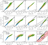 |
Fig. 5. CO intensity (top row), the HCN intensity (center row), and HCN/CO ratio (bottom row) as a function of mean gas density, velocity dispersion, kinetic temperature, and gas column density. The column densities shown are from Eq. (12) for ICO and IHCN (top and center rows) and are the fiducial model column densities for the HCN/CO ratio (bottom row). The reference conversion factor values are shown in the intensity vs. column density plots as the dotted and dashed lines. We show the CO fits (top row) in the HCN plots (center row) as the gray dashed lines. Spearman rank coefficients are shown in the lower right corner. The formatting is the same as in Fig. 3. We plot fits from the results of the ALMOND survey (purple dotted line, Neumann et al. 2023) and Tafalla et al. (2023, red dashed line). Uncertainties on their respective fits are shown as the shaded areas. For comparison, we plot the results of Paper I sample (solid contours) and the EMPIRE sample (dashed contours, Jiménez-Donaire et al. 2019) in the HCN/CO ratio vs. gas surface density plot. Our models show strong positive correlations between the modeled line intensities and mean density, velocity dispersion, mean kinetic temperature, and gas column densities. IHCN appears to increase more rapidly with each of these parameters compared to ICO. The Spearman rank coefficients are shown in the lower right corner of each plot. |
We find a relationship between IHCN/ICO and gas surface density in our models (cf. Fig. 5), which has been found in studies of gas clouds in the Milky Way (e.g., Tafalla et al. 2023) as well as nearby galaxies (e.g., Gallagher et al. 2018b; Neumann et al. 2023). We perform a fit between log(IHCN/ICO) and log of the mean gas surface density and find a sublinear relationship similar to that found by (Tafalla et al. 2023, Eq. (6)):
Uncertainties on the fit are determined using bootstrapping. Tafalla et al. (2023) find a slope of 0.71. As Tafalla et al. (2023) show, other extragalactic studies find sublinear slopes, as well (0.81 in Gallagher et al. 2018a and 0.5 in Jiménez-Donaire et al. 2019). Interestingly, the recent results of the ALMOND survey find a much shallower slope of ∼0.33 (Neumann et al. 2023). Neumann et al. (2023) compare observations of HCN and CO at 2.1 kpc scales with cloud-scale measurements of velocity dispersion and gas surface density from PHANGS galaxies, which may explain this discrepancy. We compare our fit with the results of Tafalla et al. (2023) and Neumann et al. (2023) in Fig. 5. Our fit is slightly offset from Tafalla et al. (2023), which is consistent with the offset we see in our model intensities in Fig. 3. This relationship is in part due to the gas volume density and gas surface density scaling with each other in our models (cf. Eqs. (9) and (10)), and the overall dense gas fraction increasing with gas volume density4. In general, our models are able to reproduce the sublinear relationship observed between the HCN/CO intensity ratio and gas surface density observed in both Milky Way clouds at ∼parsec scales and nearby galaxies at ∼kiloparsec scales.
In summary, our models are able to reproduce the range of HCN and CO J = 1–0 intensities measured in the disk galaxies of the EMPIRE sample (Jiménez-Donaire et al. 2019) and our more extreme sample of galaxies including U/LIRGs and galaxy centers, presented in Paper I (cf. Fig. 3). Furthermore, we show that our models reproduce the expectations of CO excitation and optical depth (cf. Bolatto et al. 2013; Narayanan et al. 2012; Narayanan & Krumholz 2014). Although HCN is less well-studied than CO, we find that our models agree with results of the current works. In particular, HCN appears subthermally excited, as has been found via studies of high−J lines of HCN emission in nearby galaxies (García-Rodríguez et al. 2023), and inferred from studies in Milky Way clouds (Dame & Lada 2023). Additionally, HCN appears only moderately optically thick (τ < 10), as was found by Jiménez-Donaire et al. (2017) when comparing HCN and H13CN emission towards the centers of nearby disk galaxies. Since gas volume density tracks column density in our models, we find IHCN/ICO also scales with gas surface density.
3.2. The fraction of gas traced by the HCN/CO ratio
We consider what fraction of gas the IHCN/ICO ratio is sensitive to in molecular clouds, and whether this changes in more extreme environments, such as those found in galaxy centers. This is motivated by previous studies which have found an increase in the dense gas depletion time towards the centers of some disk galaxies (Gallagher et al. 2018a; Querejeta et al. 2019; Jiménez-Donaire et al. 2019; Bešlić et al. 2021) and even in the nuclei of the Antennae (Bemis & Wilson 2019), despite these regions also having higher IHCN/ICO. Under the assumption that IHCN/ICO tracks the fraction of dense (n > 104.5 cm), star-forming gas in molecular clouds, those results appeared in conflict with fixed threshold models of star formation that predict star formation should turn on above a relatively fixed density, and that the star formation rate should increase in the presence of higher fdense (see the works by Usero et al. 2015; Khullar et al. 2019). In agreement with previous studies (e.g., Burkhart & Mocz 2019), Paper I shows that gravoturbulent models of star formation are able to reproduce this increase in dense gas depletion time towards regions with higher fractions of dense gas. This result agrees with the findings of Gallagher et al. (2018a), Querejeta et al. (2019), Jiménez-Donaire et al. (2019), Bešlić et al. (2021) and Bemis & Wilson (2019). The major caveats of this conclusion are: 1. that IHCN/ICO is tracing the fraction of gas above a relatively fixed density (i.e., n > 104.5 cm), and 2. that the turbulent gas velocity dispersion is also increasing with IHCN/ICO. We have already shown that IHCN/ICO increases with σv in Fig. 5. We now consider if IHCN/ICO is tracing the fraction of gas above a relatively fixed density.
In Paper I, we focus on comparing the HCN/CO ratio with the fraction of gas above n > 104.5 cm−3, which is the assumed threshold density for some clouds in the Milky Way disk. Other studies have shown that HCN is tracing gas primarily at moderate densities, n ∼ 103 cm−3 (e.g., Kauffmann et al. 2017; Pety et al. 2017; Shimajiri et al. 2017; Barnes et al. 2020; Tafalla et al. 2021, 2023; Santa-Maria et al. 2023, Ngoc Le et al. in prep.), such that it may be more sensitive to mass fractions including densities below n ∼ 104.5. We compare the modeled HCN/CO ratio to several gas fractions derived from the model n−PDFs in Fig. 6. To determine the fraction of gas above an arbitrary threshold density, we integrate the n−PDF above that threshold (nthresh):
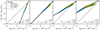 |
Fig. 6. 3.2 × IHCN/ICO as a function of the fraction of gas above (from left to right) n ∼ 102.5, 103.5, 104.5, and 105.5 cm−3. The formatting is the same as in Fig. 3. The fits are shown as the solid black line (see legend). The modeled IHCN/ICO scales most directly (has a slope closest to unity) with f(n > 103.5 cm−3), supporting previous findings that this line ratio is sensitive to gas above moderate densities. Although not shown here, the same is found when comparing the emissivity ratio, ⟨ϵHCN⟩/⟨ϵCO⟩, with the same gas fractions. The Spearman rank coefficients are shown in the lower right corner of each plot. |
We calculate gas fractions using the n−PDF above densities log (n) = 2.5, 3.5, 4.5, 5.5 cm−3, denoted by f2.5, f3.5, f4.5, and f5.5, respectively. We numerically integrate over a wide range in densities when calculating these fractions to ensure the n–PDF is fully sampled. We note that we multiply the modeled IHCN/ICO ratio by a fixed factor, αHCN/αCO = 3.2, which is the ratio of the Gao & Solomon (2004a,b) HCN-to-dense H2 mass and Milky Way CO-to-total H2 mass conversion factors, and is the same factor we have we have applied to the HCN/CO ratio measured in the sources of our sample to estimate dense gas fractions in Paper I.
We calculate Spearman rank coefficients (rs) between IHCN/ICO and the gas fractions shown in Fig. 6 (i.e., f2.5, f3.5, f4.5, and f5.5). The IHCN/ICO from our models is strongly (|rs|> 0.7) correlated with all of the gas fractions we consider, with little difference between their Spearman rank coefficients. We fit the correlations between 3.2 × IHCN/ICO and each of the fractions shown in Fig. 6 to assess the directness of each relationship. With a slope close to unity, the IHCN/ICO ratio appears to have the most direct relationship with the fraction of gas above n ∼ 103.5 cm−3. The relationship between 3.2 × IHCN/ICO and f(n > 104.5 cm−3) appears sublinear in our models, such that 3.2 × IHCN/ICO overestimates f(n > 104.5 cm−3) for the PHANGS-type clouds. These results suggest that IHCN/ICO is tracing gas above a relatively constant fraction of gas, but that this includes gas at moderate densities below n < 104.5 cm−3.
In summary, our models predict that, on average, IHCN/ICO does appear to track gas above a relatively fixed density, but that this fraction includes more moderately dense gas (i.e., n > 103.5 cm) as opposed to strictly dense gas above n > 104.5 cm. This result appears in agreement with more recent studies of HCN emission in Milky Way clouds that find HCN emission includes more moderate gas densities, for example n ∼ 800 cm−3 (e.g., Kauffmann et al. 2017). Our models include a range of cloud properties, including those found in normal galaxies (i.e., PHANGS models) as well as more extreme cloud models based on cloud properties from the Antennae and NGC 3256. We find evidence that IHCN/ICO tracks a gas fraction including more moderate gas densities even in the more extreme environments.
3.3. Using estimates of CO and HCN Emissivity to derive gas masses
We explore if the dense gas fraction can be consistently recovered from observations of HCN and CO using luminosity-to-mass conversion factors, which are commonly used to estimate molecular gas masses from molecular line observations. We recall from Sect. 2.5 that emissivity can be recast in units of luminosity-to-mass conversion factors, such that αmol ∝ 1/⟨ϵmol⟩, with the caveat that emissivities derived in this work are relative to true cloud surface densities, rather than integrated quantities such as mass and molecular line luminosity. By construction, the ratio of our modeled intensities will be proportional to the ratio of molecular line luminosities analogous to those measured in resolved or unresolved observations, or the ratio of line intensities of resolved observations. We note that for the remainder of this work, we use ⟨αmol⟩ when we are referring to the inverse of modeled emissivity of a molecular transition, and αmol when referring to an estimate of the idealised mass conversion factor of a molecular transition (which may also include additional factors, such as the filling fraction).
In Fig. 7, we present the CO and HCN emissivities from our models, and contrast these against idealised luminosity-to-mass conversion factors. We fit the relationship between ⟨αCO⟩ = 1/⟨ϵCO⟩ and ICO using orthogonal distance regression and find the following:
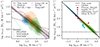 |
Fig. 7. The modeled emissivities of CO and HCN in units of M⊙ (K km s−1 pc2)−1 as a function of CO and HCN intensity, respectively. Left: Inverse of the CO emissivity (in units of the CO conversion factor) as a function of CO intensity, ⟨αCO⟩=⟨ϵCO⟩−1. We include the fit to our models (Eq. (17), solid line) and the 1σ uncertainty on the fit (gray shaded area). We also include the results of several numerical studies (Narayanan et al. 2012; Hu et al. 2022a; Gong et al. 2020, red dashed line, cyan dotted line, brown dash-dotted line, respectively) as well as the results of observational studies at ∼150 pc scales in the Antennae (pink dashed line, He et al. 2024) and PHANGS galaxies (purple dotted line, Teng et al. 2024). We note that we have recast the αCO − σv fit from Teng et al. (2024) in terms of ICO using the fit between ICO and σv from our models. Right: Inverse of the HCN emissivity (in units of the HCN conversion factor) as a function of HCN intensity, ⟨αHCN⟩=⟨ϵHCN⟩−1. We include a fit to our models (Eq. (18), solid line) and the 1σ uncertainty on the fit (gray shaded area). For comparison, we include several published values of αHCN from observations of Milky Way clouds (Dame & Lada 2023; Shimajiri et al. 2017), and we show the Gao & Solomon (2004a,b) value as the black dashed line. This figure demonstrates how well our models are able to reproduce previous numerical prescriptions of αCO, as well as observationally constrained values of αCO and αHCN. The formatting of the model output is the same as in Fig. 3. |
Uncertainties are determined using bootstrapping. We show in Fig. 7 that our CO emissivities agree well with the Narayanan et al. (2012) prescription for the CO-to-H2 conversion factor. We find a similar slope, −0.26, compared to −0.32 in Narayanan et al. (2012). We also compare with the numerical works of Hu et al. (2022a) and Gong et al. (2020). The prescription taken from Hu et al. (2022a), in particular, is for 1 kpc scales, which might explain the offset between their prescription and ours, but has roughly a similar slope (−0.43). In their work they also include modeling of αCO at higher resolution and do find higher values more consistent with our modeling. The Gong et al. (2020) relationship has a shallower slope than our trend, which appears inconsistent with some of the most recent studies of αCO in nearby galaxies (e.g., He et al. 2024; Teng et al. 2024). We also compare with observationally derived estimates of αCO at ∼150 pc scales in the Antennae (He et al. 2024) and PHANGS galaxies (Teng et al. 2024). We find good agreement with these studies. We note that we have recast the αCO − σv fit from Teng et al. (2024) in terms of ICO using the fit between ICO and σv from our models. Additionally, we find that there is little difference between 1/⟨ϵCO⟩ and our model estimates of αCO, where we divide the model column density by ICO directly. This agreement is a reflection of how well the column of mass traced by CO J = 1–0 tracks the mean H2 column density of our models, and further reinforces the utility of CO J = 1–0 as a tracer of the total molecular gas content in molecular clouds in nearby galaxies. On average, αCO decreases with increasing ICO which is a reflection of increasing CO excitation as well as variations in CO optical depth. Overall, our model estimates of ⟨αCO⟩ = 1/⟨ϵCO⟩ appear to agree well with prescriptions from numerical work (e.g., Narayanan et al. 2012) as well as recent, high-resolution studies of molecular gas in galaxies we have used as our model templates (e.g., He et al. 2024; Teng et al. 2024).
We see a similar decrease in 1/⟨ϵHCN⟩ with increasing IHCN, but find that values of 1/⟨ϵHCN⟩ span over ∼2.5 dex, while values of 1/⟨ϵCO⟩ span ∼1 dex in our models. We fit the relationship between ⟨αHCN⟩ = 1/⟨ϵHCN⟩ and IHCN using orthogonal distance regression and find
Again, uncertainties are determined using bootstrapping. We also see in Fig. 7 that the Gao & Solomon (2004a,b) value for αHCN is only consistent with the brightest IHCN in our models. Several recent studies of Milky Way clouds find evidence of larger values of αHCN relative to the original estimate by Gao & Solomon (2004a,b). An estimate of αHCN = 92 (M⊙ [K km s−1 pc2])−1 in the Perseus Molecular Cloud from Dame & Lada (2023) falls within the range of 1/⟨ϵHCN⟩ found in our models. They derive αHCN by comparing observations of HCN J = 1–0 luminosity with gas mass estimates derived from extinction measurements of dust. Dame & Lada (2023) also note that HCN brightness has a significant effect on the value of αHCN, and when the original Gao & Solomon (2004a,b) value is scaled by an HCN brightness temperature more appropriate for Galactic GMCs they derive a value more consistent with their measurement from Perseus. We also compare with the results of Shima et al. (2017) in Fig. 7, and find good agreement with the values they derive for Aquila, Ophiuchus, and Orion B. Tafalla et al. (2023) also derive estimates of αHCN in Milky Way clouds using extinction estimates. They find αHCN = 23, 46, and 73 M⊙ (K km s−1 pc2)−1 for the California, Orion A, and Perseus molecular clouds, respectively. Additionally, Forbrich et al. (2023) find evidence of deviations in αHCN from the original estimate of Gao & Solomon (2004a,b). They find αHCN ≈ 1 (M⊙ [K km s−1 pc2])−1 in six GMCs in Andromeda by comparing estimates of dust with HCN emission. When assuming the Milky way dust-to-gas mass ratio, they find a much larger value of αHCN ≈ 109 (M⊙ [K km s−1 pc2])−1, similar to that of Dame & Lada (2023). We note that the Tafalla et al. (2023) estimate for Perseus is slightly lower than that quoted by Dame & Lada (2023), which they argue is potentially from extended HCN emission not included in the mapping area of the Dame & Lada (2023) study. However, we find the opposite effect on αHCN (1/⟨ϵHCN⟩) when we exclude HCN emission from lower column densities in our models (cf. Appendix C) and conclude that this discrepancy could, in part, be due to the sensitivity limit of the Tafalla et al. (2023) study.
Despite the broader range in HCN emissivity relative to CO emissivity, we find that IHCN/ICO closely tracks the fraction of gas above n > 103.5 cm−3, which implies a nearly constant HCN and CO luminosity-to-mass ratio, αHCN/αCO, can be used to estimate f(n > 103.5 cm−3) from observations (cf. Fig. 8). Regardless of the absolute value of αHCN/αCO, the results of our modeling suggest that the fraction of gas above n > 103.5 cm−3 can be roughly estimated by applying a fixed αHCN/αCO ratio to IHCN/ICO, although this ratio appears to be larger than our initially assumed value of αHCN/αCO = 3.2. These results suggest that (1) the HCN intensity scales with the fraction of mass above moderate gas densities, and (2) a constant ratio between αHCN/αCO can be assumed to derive this fraction of gas using IHCN/ICO. Furthermore, our models predict that αHCN does not scale directly with the emissivity of HCN. This difference in behaviour between 1/⟨ϵHCN⟩ and αHCN in our models is a reflection of HCN J = 1–0 being primarily subthermally excited.
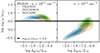 |
Fig. 8. Ratio of the HCN and CO conversion factors (given in Eq. (19)) as a function of the ratio of the HCN and CO intensities, where we consider αHCN as a conversion factor for the total mass above n > 103.5 cm−3 (left) and n > 104.5 cm−3 (right). For comparison, we plot αHCN/αCO = 3.2 (solid black line), which is the ratio of the Gao & Solomon (2004a,b) conversion factor and Milky Way CO conversion factor. The formatting is the same as in Fig. 3. This figure demonstrates how emissivity is sensitive to the intensity per mass traced by a particular transition, whereas luminosity-to-mass conversion factors account for additional factors that allow us to estimate specific masses (e.g., total gas mass and dense gas mass) that may not be fully reflected in the molecular emissivity. We find that due to the subthermal excitation of HCN J = 1–0, this transition is a poor tracer of the of the gas mass above n > 104.5 cm−3 and is a better tracer of moderate gas densities (n > 103.5 cm−3), as found in previous observational studies. |
We reframe the results above in terms of the ratio of the HCN and CO luminosity-to-mass conversion factors, αHCN/αCO by multiplying the ratio of IHCN/ICO by the fraction of mass with densities above nthresh > 103.5 cm−3 and nthresh > 104.5 cm−3, for example
Thus, when the ratio of αHCN/αCO is multiplied with IHCN/ICO, we get an estimate of said gas mass fraction:
We show these results in Fig. 8 as a function of IHCN/ICO. We find that αHCN/αCO is relatively constant when assuming IHCN tracks the mass above n > 103.5 cm−3. To derive the fraction of gas above n > 103.5 cm−3, our models predict that one can apply αHCN/αCO ≈ 5 to IHCN/ICO. Contrary to this, αHCN/αCO must increase with IHCN/ICO when assuming IHCN tracks the mass above n > 104.5 cm−3. Although not shown in Fig. 8, this relationship is even steeper when considering f(n > 105.5 cm−3). This analysis is consistent with our findings in Fig. 6, where we see that IHCN/ICO scales most directly (linearly) with the fraction of gas above n > 103.5 cm−3.
These results suggest that, in theory, the fraction of dense gas above n > 104.5 cm−3 can be derived from IHCN/ICO if one adopts a prescription for αHCN/αCO that increases with IHCN/ICO. However, our models show that estimates of dense gas mass using the original estimate of αHCN from Gao & Solomon (2004a,b) likely overestimate the true dense gas mass, except in the most extreme cases like galaxy mergers and U/LIRGs. This overestimate is more significant for disk galaxies, such as the Milky Way and galaxies in the PHANGS sample. It may be more useful to observe other molecular line transitions that are exclusively sensitive to higher gas densities, such as N2H+ (Kauffmann et al. 2017; Pety et al. 2017; Priestley et al. 2023) to estimate f(n > 104.5 cm−3), rather than attempting to calibrate the relationship between IHCN/ICO and f(n > 104.5 cm−3).
Despite HCN having a higher critical density than N2H+, N2H+ appears to more reliably trace cool, dense gas in Milky Way molecular clouds (Kauffmann et al. 2017; Pety et al. 2017; Tafalla et al. 2021), whereas HCN emission tends to originate from gas at more moderate temperatures (Pety et al. 2017; Barnes et al. 2020) and more moderate gas densities (Kauffmann et al. 2017; Pety et al. 2017). There are several chemical processes that limit N2H+ emission to regions of primarily dense, cool gas (T < 20 K). N2H+ is destroyed in the presence of CO via ion–neutral interactions (Meier & Turner 2005). Furthermore, the creation of N2H+ depends on the availability of H3+ to react with N2, which is a chemical process in competition with the creation of CO. Thus, N2H+ is primarily abundant in regions where CO is depleted onto dust grains (Caselli & Ceccarelli 2012), unlike HCN which is present also at moderate densities of gas overlapping with CO (Kauffmann et al. 2017; Pety et al. 2017). Thus, N2H+ may be a better tracer of the cold, dense gas that serves as the direct fuel for star formation.
Interestingly, Jiménez-Donaire et al. (2023) find that N2H+ and HCN have a nearly constant ratio over a large range of spatial scales. They compare observations of N2H+ and HCN in NGC 6946 at 1 kpc scales with existing literature values of other galaxies (Mauersberger & Henkel 1991; Nguyen et al. 1992; Watanabe et al. 2014; Aladro et al. 2015; Nishimura et al. 2016; Takano et al. 2019; Eibensteiner et al. 2022) and Milky Way clouds (Jones et al. 2012; Pety et al. 2017; Barnes et al. 2020; Yun et al. 2021), and find this ratio is IN2H+/IHCN = 0.15 ± 0.02 averaged over parsec scales and kiloparsec scales. Due to the segregation of N2H+ in CO-depleted regions of molecular clouds, Jiménez-Donaire et al. (2023) conclude that the linear scaling between HCN and N2H+ must be a product of the self-similarity of clouds, and that HCN emission may still be a valuable dense gas tracer to assess the properties of the cooler, denser N2H+-emitting gas. However, extragalactic observations of N2H+ are so far limited to a handful of nearby galaxies, and have yet to be completed at cloud scales. Thus, it remains an important next step to perform comparable observations of N2H+ and HCN over a large sample of cloud environments in nearby galaxies.
3.4. IHCN/ICO and the fraction of gravitationally bound gas
We explore how well the IHCN/ICO ratio tracks gravitationally bound fraction of gas (fgrav) as predicted by the LN+PL analytical models of star formation. We emphasize here that we are interested in general trends that are predicted by turbulent models of star formation, and the LN+PL analytical models of star formation (Burkhart 2018) agree closely with those of the LN-only models (Krumholz & McKee 2005; Padoan & Nordlund 2011). As such, we only compare against the results of the LN+PL analytical models of star formation.
In Fig. 9, we plot the modeled IHCN/ICO ratio and dense gas fraction, f(n > 104.5 cm−3) against fgrav. We take fgrav to be the fraction of gas in the power-law component of the LN+PL model (see Eq. (20) in Burkhart & Mocz 2019). We find that IHCN/ICO has a strong, negative correlation with fgrav. This is consistent with the results of Paper I, where we made a similar conclusion without including radiative transfer in our analysis. f(n > 104.5 cm−3) has an even steeper, negative correlation with fgrav. We note that the primary driver of the decrease in fgrav towards higher IHCN/ICO and f(n > 104.5 cm−3) is a reflection of the higher gas velocity dispersion in these models (which correspond to models with higher gas surface density and wider n–PDFs). We also find that models with the lowest estimates of fgrav and highest f(n > 104.5 cm−3) have the shortest depletion times, and the corresponding modeled IHCN/ICO and predicted depletion times are consistent with our data (cf. Fig. 9). In general, the models of star formation we consider predict that turbulence acts as a supportive process that prevents gravitational collapse of gas. Indeed, we find that the transition density (the density at which gas becomes self-gravitating in our models) increases across our model parameter space from n = 104.5 cm−3 in the PHANGS-type models to n = 105.9 cm−3 and n = 106.6 cm−3 in the NGC 4038/9- and NGC 3256-type models, respectively. We also note that the transition density for the PHANGS-type models agrees well with the estimation for the threshold density for star formation in the Milky Way (e.g., n ≳ 104 cm−3, Lada et al. 2010, 2012).
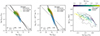 |
Fig. 9. The relationships between modeled IHCN/ICO, f(n > 104.5 cm−3), fgrav, and tdep. Left: Modeled IHCN/ICO as a function of the gravitationally bound fraction of gas (fgrav) predicted by the LN+PL analytical models of star formation. Center: Fraction of dense gas above n > 104.5 cm−3 as a function of the gravitationally bound fraction of gas (fgrav) predicted by the LN+PL analytical models of star formation. The formatting is the same as in Fig. 3. The Spearman rank coefficients are shown in the lower right corner of the left and center panels. Right: Total gas depletion time (tdep) as a function of IHCN/ICO ratio. The models are shown as colored points. The measurements of tdep and IHCN/ICO from our sample of galaxies and the EMPIRE sample are shown as the solid black and dashed black contours, respectively. Our models find that the IHCN/ICO ratio is negatively correlated with fgrav as predicted by gravoturbulent models of star formation. Additionally, the fraction of dense gas above n > 104.5 cm−3 has an even steeper negative correlation with fgrav, as predicted by gravoturbulent models of star formation (e.g., Burkhart 2018; Burkhart & Mocz 2019). Thus, although IHCN/ICO is sensitive to gas above moderate densities, we conclude that a single molecular line ratio, such as HCN/CO, does not necessarily scale with the fraction of directly star-forming gas in clouds. We also find that models with the lowest estimates of fgrav and highest f(n > 104.5 cm−3) have the shortest depletion times, and the corresponding modeled IHCN/ICO and predicted depletion times are consistent with our data. |
We also show in Fig. 9 that models with higher IHCN/ICO and lower fgrav are, on average, still consistent with observations and have overall shorter total gas depletion times (tdep), as is also seen in observations and is in agreement with the results of Paper I. The above results also have important implications for the interpretation of dense gas depletion times. These results support that the longer tdep, dense observed towards higher IHCN/ICO in our data (assuming fixed αHCN/αCO) do not necessarily imply lower star formation efficiencies of the directly star-forming gas, but rather that a lower fraction of the dense gas is unstable to collapse in these systems (see right panel of Fig 9). We confirm that fgrav is predicted to decrease from 1.7% in the PHANGS-type models to 0.8% and 0.6% in the NGC 4038/9- and NGC 3256-type models, respectively. In contrast to this, the fraction of dense gas above n = 104.5 cm−3 increases from 1.9% in the PHANGS-type models to 22% and 30% in the NGC 4038/9- and NGC 3256-type models, respectively. It is also interesting to note that in the PHANGS-type models fgrav is well-matched to fdense.
3.5. The impact of CO and HCN emissivity on star formation relations
We consider here how variations in emissivity can impact the scatter as well as the general trends of some star formation relations. One of the differences between the results shown in Paper I and this work is the origin of the scatter in the various star formation scaling relationships. In Paper I, the scatter produced in the modeled star formation scaling relationships is partially from changes in ϵff due to variations in PL slope for the LN+PL models or variations in turbulence (quantified by the sonic Mach number) for the LN-only models. In this work, we also show that variations in the emissivity of CO contribute to and may even account for the majority of the scatter in observational star formation scaling relationships.
For example, we show in Fig. 10 that the modeled trend in ϵff with Pturb agrees well with observations under the assumption of a fixed αCO and assuming mean density scales with gas surface density. We plot ϵff versus Pturb using method one described at the beginning of the results section, which is analogous to the method used to derive gas surface densities from observations. For comparison, we also plot tdep as a function of the HCN/CO ratio in Fig. 10. In these two plots the scatter in our models primarily comes from variations in CO intensity (since we have fixed PL slope). The scatter is also correlated with variations in CO emissivity. This is apparent in the gradient in ⟨αCO⟩ = 1/⟨ϵCO⟩ across the colored points in the left two panels of Fig. 10. Models with lower CO intensity (which in general have higher αCO and lower CO emissivity, see Fig. 7) appear to have higher ϵff and vice versa (Fig. 10). This agrees with the trend we observe in our data in Bemis & Wilson (2023) (also shown in Fig. 10) where we have adopted a fixed CO conversion factor and assumed mean gas density scales with gas surface density. These results show that variations in CO emissivity can account for a significant amount of scatter observed in star formation scaling relations. When we apply ⟨αCO⟩ = 1/⟨ϵCO⟩ to our modeled ICO to estimate gas surface density (while still using the assumption that the mean gas volume density scales with with gas surface density), we produce tighter trends in ϵff with Pturb and tdep with HCN/CO (purple lines) that are qualitatively more consistent with the actual model predictions (red lines, left two panels of Fig. 10). The offset in ϵff and tdep between the model prediction and what is obtained when we apply ⟨αCO⟩ = 1/⟨ϵCO⟩ to our modeled ICO in Fig. 10 is a result of modeled CO emission missing a fraction of the lower surface density gas in our models, analogous to CO-dark gas (cf. Bolatto et al. 2013). When we scale ⟨ϵCO⟩−1 by the ratio between the true model gas surface density and ⟨NCO⟩ we find nearly identical trends.
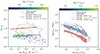 |
Fig. 10. Comparisons between theoretical predictions and our radiative transfer modeling of the relationships between ϵff, Pturb, tdep, and IHCN/ICO. Left: Model efficiency per free-fall time as a function of turbulent pressure shown three ways: (1) using modeled ICO and a fixed CO conversion factor for gas surface density estimates (colored points), (2) using the actual theoretical ϵff and Pturb values (red line), and (3) using modeled ICO with ⟨αCO⟩ = 1/⟨ϵCO⟩ (purple trend line). The shaded regions represent the full range of model scatter. Estimates of these quantities from our sample of galaxies and the EMPIRE sample are shown as the solid black and dashed black contours, respectively. Right: Model depletion time as a function of HCN/CO ratio shown three ways, using the same approach. We find that the scatter produced by variations in CO emissivity can account for a significant portion of the scatter seen in observations. Additionally, the trend in ϵff with Pturb is dependent on the assumed CO conversion factor. Pixel-by-pixel estimates of αCO may be necessary for accurate studies of star formation trends. We note that the offset in ϵff and tdep between methods (2) and (3) is a result of the modeled CO emission missing a fraction of the lower surface density gas in our models, to CO-dark gas. |
We quantify the scatter in ϵff vs. Pturb by fitting a line to the relationship and calculating the standard deviation on the y−residuals. Assuming constant conversion factors, the scatter in the ϵff vs. Pturb relationship is ∼0.36 using method one and becomes ∼0.05 when we apply ⟨αCO⟩ = 1/⟨ϵCO⟩, which is similar to the scatter in the theoretical prediction (∼0.02). The scatter in tdep with HCN/CO is ∼0.21 when assuming constant conversion factors and becomes ∼0.12 when we apply ⟨αCO⟩ = 1/⟨ϵCO⟩. The scatter in the theoretical prediction is ∼0.18. We conclude that a significant portion of the scatter in these relationships originates from variations in emissivity in our models.
We calculate Spearman rank coefficients (rs) between ⟨αCO⟩ = 1/⟨ϵCO⟩ and ⟨τCO⟩, ⟨Tex, CO⟩, σv, Σmol, n0, Tkin, and ⟨ICO⟩ to assess the strength of the correlation between these parameters. We find that ⟨αCO⟩ only strongly (|rs|> 0.7) correlates with ⟨τCO⟩ (rs = 0.9) in our models. ⟨αCO⟩ is moderately (0.5 < |rs|< 0.7) correlated with σv (rs = −0.6) and ⟨ICO⟩ (rs = −0.5). αCO is weakly (|rs|< 0.5) correlated with the remainder of the parameters (⟨Tex, CO⟩, Σ, n0, and Tkin). This suggests that variations in CO emissivity are primarily driven by changes in optical depth in our models. Furthermore, the connection between ⟨αCO⟩ and ⟨τCO⟩ likely stems from variations in gas velocity dispersion, since higher gas velocity dispersions are connected to lower optical depths in our models and higher CO intensities, as shown in Fig. 4. This also explains the variations we see in ⟨αCO⟩, for example in the scatter of ϵff with Pturb and tdep with HCN/CO, since the scatter of our model parameter space (shown in Fig. 2) is set by variations in velocity dispersion. We can also conclude that variations in ⟨αCO⟩ are, to a lesser effect, driven by variations in the mean gas density that the CO emission originates from, but ⟨αCO⟩ is more strongly correlated with Tkin (rs = −0.4) relative to n0 (rs = −0.2) in our models. We note that CO emissivity is also impacted by the width of the n–PDF, which is set by a combination of the turbulent velocity dispersion and gas kinetic temperature in our models. Thus, inconsistencies between observationally derived quantities and model predictions, such as ϵff, may in part be due to uncertainties in mean gas density, but are also likely driven by a number of other quantities (i.e., gas velocity dispersion and kinetic temperature) that we expect to vary consistently across trends in star formation.
Recent work on the Antennae (He et al. 2024) shows that αCO in this system has a negative correlation with their measurements of velocity dispersion. They make a similar argument that αCO may have a connection to the dynamics of the gas. He et al. (2024) find a strong, positive correlation between αCO and τCO. We note that optical depth has a dependence on σv and gas surface density (τCO ∝ σv/Σ). Thus, these results suggest some variations in the dynamics of the gas also impact CO optical depth, which is reflected in αCO. The importance of dynamics has also been discussed in earlier works by Solomon et al. (1987), and Solomon et al. (1997), Gao & Solomon (1999).
Work on the PHANGS galaxies at 150 pc scales shows there is a negative correlation between αCO and velocity dispersion which appears to have lower scatter (∼0.1 dex) relative to previous prescriptions relying on gas or stellar surface density (Teng et al. 2024). They also argue that this correlation is tied to variations in emissivity of CO. We note that Teng et al. (2024) find a slightly steeper correlation than He et al. (2024) (slope −0.81 vs. −0.46, respectively). When we fit this relationship in our models, we find a slope of ∼−0.5, more consistent with the Antennae relationship. When we estimate the scatter relative to our fit, we find ∼0.16 dex, similar that found by Teng et al. (2024), 0.12 dex. In summary, our models are able to reproduce the negative correlation between αCO and σv seen in high-resolution studies of PHANGS galaxies and the Antennae and can produce similar scatter. Furthermore, the physical origin of the variations in CO emissivity in the scatter of our models can be interpreted as arising from variations in optical depth tied to the dynamics of the gas, analogous to what is observed across the Antennae and PHANGS galaxies (i.e., He et al. 2024; Teng et al. 2024).
Additionally, we find that uncertainties in CO emissivity can lead to different slopes in star formation scaling relations that can have significantly different implications. In Paper I, we find a discrepancy between the predictions of gravoturbulent models of star formation and observations such that ϵff is predicted to increase with Pturb by these models, but observations instead show a decrease in ϵff with Pturb. We also show this in Fig. 10, where we plot the model-predicted ϵff as a function of Pturb, using the actual mean gas volume density to estimate tff and therefore ϵff (as well as Pturb). In Paper I, we assume this discrepancy between our data and model predictions arises from uncertainties in mean volume density and our assumption that mean volume density scales with gas surface density (see Fig. 7 in Paper I). In Fig. 10, we show that all model estimates of tdep as a function of the HCN/CO ratio have a negative trend, highlighting that this effect may be most important for observational relationships where subtle trends are expected. For example, the theoretical prediction for ϵff as a function of Pturb in our models has a slope of only ∼0.05, and while our models (and data) show negative slopes around ∼−0.27. This comparison suggests that accurate pixel-by-pixel estimates of CO emissivity are required to derive much more accurate star formation scaling relations from observations. Such estimates can be derived via resolved studies of molecular line transitions with independent mass estimates, such as those derived from dust.
Finally, we plot tdep, dense as a function of the HCN/CO ratio in Fig. 11 to consider how variations in HCN emissivity may impact observations of star formation relations. Interestingly, we do not see the same variation of the HCN emissivity in the scatter in tdep, dense as a function of the HCN/CO ratio that we see in CO emissivity in Fig. 10. This is likely because variations in HCN emissivity are more strongly driven by HCN excitation, and only weakly driven by optical depth in our models. When we calculate the Spearman rank coefficient between ⟨αHCN⟩ = 1/⟨ϵHCN⟩ and the same paramaters that we consider for CO, we find αHCN is strongly correlated (|r|≥0.95) with ⟨Tex, HCN⟩, σv, Σ, n0, Tkin, ⟨IHCN⟩ and only weakly correlated with ⟨τHCN⟩ (rs = 0.21). This further supports the idea that variations in HCN emissivity will not necessarily closely track variations in CO emissivity in observations.
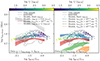 |
Fig. 11. Comparisons between theoretical predictions and our radiative transfer modeling of the relationships between tdep, dense and IHCN/ICO. Left: Model dense gas depletion time as a function of HCN/CO ratio shown three ways: (1) using modeled IHCN and a fixed HCN conversion factor for gas surface density estimates (colored points), (2) using the theoretical depletion time of the fraction of gas above n > 103.5 cm−3 (red line), and (3) using modeled IHCN with ⟨αHCN⟩ = 3.2⟨αCO⟩ applied to estimate dense gas surface density (purple line). We also show the resulting trend using modeled IHCN with ⟨αHCN⟩ = 1/⟨ϵHCN⟩ (gray dashed line) for comparison. Right: Model dense gas depletion time plotted as a function of HCN/CO ratio shown three ways, this time overlaying depletion times of several fractions of gas: that above n > 102.5, 103.5, 104.5, 105.5, cm−3 (blue, red, green, and orange lines, respectively) as a function of the HCN/CO ratio. The shaded regions represent the full range of model scatter. We find that the HCN emissivity does not appear to contribute to the scatter of these relationships in the way that CO contributes to those in Fig. 10, which is likely due to the stronger dependence of HCN emissivity on excitation relative to optical depth. Additionally, the trend in dense gas depletion time with the HCN/CO ratio depends critically on the assumed HCN conversion factor. This figure also demonstrates that the HCN emissivity does not necessarily track the mass of star-forming gas (gray trend in the left panel), but that applying ⟨αHCN⟩ = 3.2⟨αCO⟩ to IHCN when estimating tdep, dense does a reasonable job at reproducing the depletion time of gas above moderate gas densities (red lines, both panels; see also Figs. 6 and 7 and Sect. 3.4). |
Following our discussion in Sect. 3.2 (the HCN/CO ratio tracks the fraction of gas above n ≳ 103.5 cm−3) and Sect. 3.3 (application of a constant ratio in αHCN/αCO may still roughly yield f(n ≳ 103.5 cm−3)), we consider how applying ⟨αHCN⟩ = 3.2/⟨ϵCO⟩ to IHCN impacts the observed trend in tdep, dense as a function of the HCN/CO ratio and how that compares to tdep(n > 103.5 cm−3). Assuming constant αHCN, the scatter in tdep, dense as a function of the HCN/CO is ∼0.21 and becomes ∼0.12 when we apply ⟨αHCN⟩ = 3.2/⟨ϵCO⟩. This scatter in the relationship between the predicted tdep(n > 103.5 cm−3) and modeled HCN/CO ratio is ∼0.18. When applying ⟨αHCN⟩ = 3.2/⟨ϵCO⟩, the trend in tdep, dense as a function of the HCN/CO agrees well with the predicted tdep(n > 103.5 cm−3) and modeled HCN/CO ratio. To highlight this agreement, we also show a plot of tdep, dense as a function of the HCN/CO ratio in Fig. 10 compared against depletion times of different fractions of gas (i.e., n > 102.5, 103.5, 104.5, 105.5 cm−3). Lower cuts in gas density produce shallow or negative relationships, while higher cuts produce steeper relationships. We also emphasize that the HCN/CO intensity ratio still appears to track a fairly constant fraction of gas, which in our models is at moderate gas densities (n > 103.5 cm−3). Thus, assuming a constant ratio in the conversion factors of HCN and CO (e.g., ⟨αHCN⟩ = 3.2/⟨ϵCO⟩) may still be useful for determining the fraction of gas above this density.
We conclude that variations in HCN emissivity do not contribute significantly to the scatter of the considered star formation relationships. The scatter (e.g., in ϵff and tdep as a function of Pturb and tdep, dense as a function of HCN/CO ratio) primarily originates from variations in gas velocity dispersion in our models, which has a stronger effect on CO emissivity relative to HCN emissivity. This does not exclude the possibility of variations in HCN emissivity occuring in the scatter of real observations. We do expect variations in HCN emissivity in the case where variations in the physical conditions of the gas (i.e., mean gas density and kinetic temperature) impact the excitation of HCN. Due to the strong dependence of HCN emissivity on excitation, it is necessary to perform multi-line studies of HCN to assess variations of this quantity. It still remains a challenge to determine a method for assessing the fraction of star-forming gas in molecular clouds in nearby galaxies, which may ultimately require highly resolved studies of star-forming gas clouds.
4. Discussion and conclusions
In this work we explored the properties of HCN and CO emission across a range of cloud models with realistic gas density distributions, and we combined the results of this analysis with the predictions of gravoturbulent models of star formation. Our models use measurements of cloud properties based on observations of CO emission in nearby galaxies and incorporate a range of heating and cooling mechanisms to produce realistic gas temperatures (Sharda & Krumholz 2022). This prescription also includes the impact of radiation feedback from active star formation via the dust-gas energy exchange, which is important for star-forming clouds (cf. Sharda & Krumholz 2022). Our models span cloud properties found in Milky Way-type clouds (e.g., some of the PHANGS-type models of our study) through to more extreme cloud models, based on cloud properties measured in the Antennae and NGC 3256. We also incorporated radiative transfer (RADEX, van der Tak et al. 2007) in order to calculate emissivities corresponding to these cloud models. This analysis allowed us to constrain the impact of various physical properties (e.g., excitation, optical depth, mean density, velocity dispersion, temperature) on observed emission from CO and HCN across a broad range of galactic environments. Furthermore, we evaluated the sensitivity of the HCN-to-CO ratio to different gas densities, and to the fraction of gravitationally bound star-forming gas, as predicted by analytic models of star formation (e.g., Burkhart 2018; Burkhart & Mocz 2019, which we used for this work, and also see, e.g., Krumholz & McKee 2005; Federrath & Klessen 2012; Hennebelle & Chabrier 2011; Burkhart 2018, for which the results are still broadly applicable). Below we provide an itemized summary as well as a brief discussion of the primary scientific results from this work:
-
Simple models of clouds that combine realistic gas volume density distributions with radiative transfer are successful at reproducing observed IHCN/ICO ratios (cf. Sect. 2 and Figs. 1 and 3; see also Leroy et al. 2017b; Shirley 2015). Furthermore, they are successful at reproducing CO and HCN emissivities, optical depths, and trends in excitation that have been constrained from numerical work (cf. Sect. 3.1 and Figs. 4 and 5; Narayanan et al. 2012; Narayanan & Krumholz 2014; Gong et al. 2020; Hu et al. 2022a). Additionally, we find agreement between the trends in our model CO and HCN emissivities as a function of CO and HCN intensity and observationally derived values of the CO and HCN conversion factors in nearby galaxies and Milky Way clouds (cf. Sect. 3.3 and Fig 7; Teng et al. 2024; He et al. 2024; Dame & Lada 2023; Shimajiri et al. 2017; Tafalla et al. 2023).
-
IHCN/ICO is linearly correlated with the fraction of gas above moderate gas densities (e.g., n ∼ 103.5 cm−3), and the relationship between IHCN/ICO and the fraction of dense gas above n ∼ 104.5 cm−3 is sublinear in our models (cf. Sect. 3.2 and Fig. 6). Thus, our models predict that IHCN/ICO traces the fraction of gas above a roughly constant, moderate gas density, in agreement with the results of previous studies (e.g., Kauffmann et al. 2017; Pety et al. 2017), and this ratio is still useful in the determination of the fraction of gas above moderate densities (cf. Fig. 11). One can still apply a roughly constant ratio in the HCN and CO conversion factors to IHCN/ICO to estimate f(n ∼ 103.5 cm−3), for example. This is roughly αHCN/αCO ≈ 5 in our models.
-
The modeled IHCN/ICO and HCN/CO emissivity ratios are negatively correlated with fgrav, as predicted by gravoturbulent models of star formation with varying star formation thresholds (cf. Sect. 3.4 and Fig. 9). Thus, models with the lowest estimates of fgrav appear to have the highest dense gas fractions (i.e., f(n > 104.5 cm−3)) and highest IHCN/ICO. We find that fgrav is predicted to decrease from 1.7% in the PHANGS-type models to 0.8% and 0.6% in the NGC 4038/9-type and NGC 3256-type models, respectively. In contrast to this, the fraction of dense gas above n = 104.5 cm−3 increases from 1.9% in the PHANGS-type models to 22% and 30% in the NGC 4038/9- and NGC 3256-type models, respectively. The transition density (the density at which gas becomes self-gravitating in our models) increases across our model parameter space from n = 104.5 cm−3 in the PHANGS-type models to n = 105.9 cm−3 and n = 106.6 cm−3 in the NGC 4038/9- and NGC 3256-type models, respectively. Thus, in the PHANGS-type models fgrav is well matched to fdense, and the transition density for the PHANGS-type models agrees well with the estimation for the threshold density for star formation in the Milky Way (e.g., n ≳ 104 cm−3, cf. Sect. 3.4, Lada et al. 2010, 2012).
-
Models with the lowest estimates of fgrav (highest f(n > 104.5 cm−3) and highest IHCN/ICO) appear to have the shortest gas depletion times (i.e., the NGC 4038/9- and NGC 3256-type models). Thus, lower fgrav does not necessarily mean longer depletion times in the case where sufficient mass is available to star formation. We find that the trend in the modeled gas depletion times and IHCN/ICO are consistent with the trend observed in our data (cf. Sect. 3.4 and Fig. 9).
-
The scatter observed in star formation trends, such as ϵff and tdep as a function of Pturb and HCN/CO ratio, can largely be attributed to variations in CO emissivity. We find that the scatter in these relationships is reduced by a factor of ∼2–3 when we apply modeled CO emissivity to ICO to estimate gas surface density (relative to the assumption of a fixed CO conversion factor). We find variations in CO emissivity are primarily driven by variations in the optical depth of CO due to the dynamics of the gas (cf. Sect. 3.5 and Fig. 10). We do not see the same variations in HCN emissivity in the scatter of tdep, dense as a function of HCN/CO ratio, and find that HCN emissivity is more strongly correlated with excitation. Thus, variations in HCN and CO emissivity have different physical origins according to our models (cf. Figs. 9 and 11).
-
The assumption of constant conversion factors can alter the slope of star formation trends, which is particularly important for trends with subtle slopes. For example, we find the assumption of a constant CO conversion factor can produce a negative trend in ϵff with turbulent pressure (slope ∼−0.27) in our models that also agrees with the negative trend we find in our sample in Paper I. Our models predict that the actual trend in ϵff with turbulent pressure is marginally positive (∼0.05, cf. Fig. 10).
A key prediction of our models is that, on average, IHCN/ICO does appear to track gas above a relatively fixed density. However, this fraction includes more moderately dense gas (i.e., n > 103.5 cm) as opposed to strictly dense gas above n > 104.5 cm. This conclusion generally agrees with more recent studies of HCN emission in Milky Way clouds that find HCN emission includes more moderate gas densities (e.g., Kauffmann et al. 2017; Pety et al. 2017). We find evidence that IHCN/ICO tracks a gas fraction including more moderate gas densities even in the more extreme environments. This analysis implies that previous estimates of dense gas fractions likely overestimate the true fraction of gas above n > 104.5.
Furthermore, we show that the fraction of gravitationally bound gas, as predicted by turbulent models of star formation (i.e., Burkhart 2018; Burkhart & Mocz 2019, which we use in this work, and also see, e.g., Krumholz & McKee 2005; Federrath & Klessen 2012; Hennebelle & Chabrier 2011; Burkhart 2018), decreases with IHCN/ICO. This result agrees with Paper I, and combined with the subthermal excitation of HCN, suggests that it may not be appropriate to interpret IHCN/ICO as a straightforward tracer of the dense gas associated with ongoing star formation in galaxies. While IHCN/ICO does scale with the fraction of moderate to high density gas, this is not necessarily equivalent to the fraction of gas contributing to star formation, especially in more extreme environments.
A critical observational uncertainty in the study of gas traced by HCN in extragalactic systems is the lack of observational constraints on the HCN conversion factor. Most observational prescriptions assume that HCN is optically thick, but as we show with our modeling, HCN appears only moderately thick, and these findings are consistent with the study of HCN and H13CN in the centers of nearby galaxies (Jiménez-Donaire et al. 2017). Additionally, we also show that HCN is primarily subthermally excited, which also agrees with the recent findings of HCN emission in Perseus by Dame & Lada (2023). Despite these complications, it may still be possible to use HCN as a tracer of dense gas. Recent work shows that on galactic scales, the ratio of HCN to N2H+ is nearly constant (Jiménez-Donaire et al. 2023). Since N2H+ has been shown to be a tracer of even denser gas than that traced by HCN (Kauffmann et al. 2017; Pety et al. 2017; Priestley et al. 2023), it may indicate that it is still possible to calibrate a conversion between HCN luminosity and total dense gas mass in molecular clouds.
One potential limitation of the use of an HCN conversion factor is if the fraction of dense gas mass does not increase linearly with the total mass of molecular clouds. Our models show that the ratio of the CO to HCN conversion factors, αHCN/αCO, would need to increase with IHCN/ICO for IHCN to accurately trace the fraction of gas n > 104.5 cm−3 predicted by an n–PDF with both a lognormal and power-law component. This result needs to be confirmed through more resolved studies of molecular clouds, particularly in the Milky Way. It is crucial to map the density structure down to small scales in clouds and directly compare this with mappings of multiple molecular line transitions over a range of cloud types (e.g., Dame & Lada 2023; Tafalla et al. 2023; Shimajiri et al. 2017). Including an analysis of the distribution of gas densities can also shed light on the physics of molecular clouds, and how much dense star-forming gas there is in relation to various molecular line emissivities. Additionally, multi-line studies targeting higher-J transitions are necessary to constrain the mean volume density and gas temperature traced by a particular molecular species, which are also important for determining total gas masses.
On larger scales (∼ 1 kpc), Bacchini et al. (2019) find n0 ∝ Σ0.6 in nearby spiral galaxies; however, on these scales the contribution from HI becomes significant.
We note that simulations find that gas volume density tracks column densities in molecular clouds (cf. Priestley et al. 2023).
Acknowledgments
We thank the anonymous referee for their comments and feedback on the manuscript which improved this work. Part of this work was supported by an Ontario Trillium Scholarship. The research of CDW is supported by grants from the Natural Sciences and Engineering Research Council of Canada and the Canada Research Chairs program. PS is supported by the Leiden University Oort Fellowship and the International Astronomical Union – Gruber Foundation Fellowship. IDR is supported by the Banting Fellowship program. This paper makes use of the following ALMA data: ADS/JAO.ALMA#2011.0.00467.S, ADS/JAO.ALMA#2011.0.00525.S, ADS/JAO.ALMA#2011.0.00772.S, ADS/JAO.ALMA#2012.1.00165.S, ADS/JAO.ALMA#2012.1.00185.S, ADS/JAO.ALMA#2012.1.01004.S, ADS/JAO.ALMA#2013.1.00218.S, ADS/JAO.ALMA#2013.1.00247.S, ADS/JAO.ALMA#2013.1.00634.S, ADS/JAO.ALMA#2013.1.00885.S, ADS/JAO.ALMA#2013.1.00911.S, ADS/JAO.ALMA#2013.1.01057.S, ADS/JAO.ALMA#2015.1.00993.S, ADS/JAO.ALMA#2015.1.01177.S, ADS/JAO.ALMA#2015.1.01286.S, ADS/JAO.ALMA#2015.1.01538.S. ALMA is a partnership of ESO (representing its member states), NSF (USA) and NINS (Japan), together with NRC (Canada), MOST and ASIAA (Taiwan), and KASI (Republic of Korea), in cooperation with the Republic of Chile. The Joint ALMA Observatory is operated by ESO, AUI/NRAO and NAOJ. This work made use of the following software: RADEX (van der Tak et al. 2007), ASTROPY (Astropy Collaboration 2013, 2018, 2022), PANDAS (Wes McKinney 2010; Pandas development team 2020), MATPLOTLIB (Hunter 2007), NUMPY (Harris et al. 2020), and SCIPY (Virtanen et al. 2020).
References
- Aladro, R., Martín, S., Riquelme, D., et al. 2015, A&A, 579, A101 [NASA ADS] [CrossRef] [EDP Sciences] [Google Scholar]
- Ao, Y., Henkel, C., Menten, K. M., et al. 2013, A&A, 550, A135 [NASA ADS] [CrossRef] [EDP Sciences] [Google Scholar]
- Astropy Collaboration (Robitaille, T. P., et al.) 2013, A&A, 558, A33 [NASA ADS] [CrossRef] [EDP Sciences] [Google Scholar]
- Astropy Collaboration (Price-Whelan, A. M., et al.) 2018, AJ, 156, 123 [Google Scholar]
- Astropy Collaboration (Price-Whelan, A. M., et al.) 2022, ApJ, 935, 167 [NASA ADS] [CrossRef] [Google Scholar]
- Bacchini, C., Fraternali, F., Iorio, G., & Pezzulli, G. 2019, A&A, 622, A64 [NASA ADS] [CrossRef] [EDP Sciences] [Google Scholar]
- Ballesteros-Paredes, J., Vázquez-Semadeni, E., Gazol, A., et al. 2011, MNRAS, 416, 1436 [NASA ADS] [CrossRef] [Google Scholar]
- Barnes, J. E., & Hernquist, L. 1996, ApJ, 471, 115 [NASA ADS] [CrossRef] [Google Scholar]
- Barnes, A. T., Kauffmann, J., Bigiel, F., et al. 2020, MNRAS, 497, 1972 [NASA ADS] [CrossRef] [Google Scholar]
- Beattie, J. R., Mocz, P., Federrath, C., & Klessen, R. S. 2021, MNRAS, 504, 4354 [NASA ADS] [CrossRef] [Google Scholar]
- Beetz, C., Schwarz, C., Dreher, J., & Grauer, R. 2008, Phys. Lett. A, 372, 3037 [NASA ADS] [CrossRef] [Google Scholar]
- Bemis, A., & Wilson, C. D. 2019, AJ, 157, 131 [NASA ADS] [CrossRef] [Google Scholar]
- Bemis, A. R., & Wilson, C. D. 2023, ApJ, 945, 42 [NASA ADS] [CrossRef] [Google Scholar]
- Bešlić, I., Barnes, A. T., Bigiel, F., et al. 2021, MNRAS, 506, 963 [CrossRef] [Google Scholar]
- Bigiel, F., Leroy, A., Walter, F., et al. 2008, AJ, 136, 2846 [NASA ADS] [CrossRef] [Google Scholar]
- Bigiel, F., Leroy, A. K., Blitz, L., et al. 2015, ApJ, 815, 103 [NASA ADS] [CrossRef] [Google Scholar]
- Bolatto, A. D., Wolfire, M., & Leroy, A. K. 2013, ARA&A, 51, 207 [CrossRef] [Google Scholar]
- Bournaud, F., Duc, P. A., & Emsellem, E. 2008, MNRAS, 389, L8 [NASA ADS] [CrossRef] [Google Scholar]
- Brunetti, N., & Wilson, C. D. 2022, MNRAS, 515, 2928 [NASA ADS] [CrossRef] [Google Scholar]
- Brunetti, N., Wilson, C. D., Sliwa, K., et al. 2021, MNRAS, 500, 4730 [Google Scholar]
- Brunetti, N., Wilson, C. D., He, H., et al. 2024, MNRAS, 530, 597 [NASA ADS] [CrossRef] [Google Scholar]
- Brunt, C. M. 2010, A&A, 513, A67 [NASA ADS] [CrossRef] [EDP Sciences] [Google Scholar]
- Brunt, C. M., Federrath, C., & Price, D. J. 2010a, MNRAS, 405, L56 [CrossRef] [Google Scholar]
- Brunt, C. M., Federrath, C., & Price, D. J. 2010b, MNRAS, 403, 1507 [Google Scholar]
- Burkhart, B. 2018, ApJ, 863, 118 [CrossRef] [Google Scholar]
- Burkhart, B., & Lazarian, A. 2012, ApJ, 755, L19 [NASA ADS] [CrossRef] [Google Scholar]
- Burkhart, B., & Mocz, P. 2019, ApJ, 879, 129 [NASA ADS] [CrossRef] [Google Scholar]
- Burkhart, B., Stanimirović, S., Lazarian, A., & Kowal, G. 2010, ApJ, 708, 1204 [NASA ADS] [CrossRef] [Google Scholar]
- Burkhart, B., Ossenkopf, V., Lazarian, A., & Stutzki, J. 2013, ApJ, 771, 122 [NASA ADS] [CrossRef] [Google Scholar]
- Burkhart, B., Stalpes, K., & Collins, D. C. 2017, ApJ, 834, L1 [Google Scholar]
- Caselli, P., & Ceccarelli, C. 2012, A&ARv, 20, 56 [Google Scholar]
- Chakrabarti, S., & McKee, C. F. 2005, ApJ, 631, 792 [NASA ADS] [CrossRef] [Google Scholar]
- Chen, H., Gao, Y., Braine, J., & Gu, Q. 2015, ApJ, 810, 140 [NASA ADS] [CrossRef] [Google Scholar]
- Chen, H. H.-H., Pineda, J. E., Offner, S. S. R., et al. 2019, ApJ, 886, 119 [Google Scholar]
- Choudhury, S., Pineda, J. E., Caselli, P., et al. 2021, A&A, 648, A114 [NASA ADS] [CrossRef] [EDP Sciences] [Google Scholar]
- Crocker, R. M., Krumholz, M. R., & Thompson, T. A. 2021, MNRAS, 503, 2651 [CrossRef] [Google Scholar]
- Dame, T. M., & Lada, C. J. 2023, ApJ, 944, 197 [NASA ADS] [CrossRef] [Google Scholar]
- Dib, S., Brandenburg, A., Kim, J., Gopinathan, M., & André, P. 2008, ApJ, 678, L105 [Google Scholar]
- Downes, D., Solomon, P. M., & Radford, S. J. E. 1993, ApJ, 414, L13 [NASA ADS] [CrossRef] [Google Scholar]
- Draine, B. T. 2011, Physics of the Interstellar and Intergalactic Medium (Princeton: Princeton University Press) [Google Scholar]
- Eibensteiner, C., Barnes, A. T., Bigiel, F., et al. 2022, A&A, 659, A173 [CrossRef] [EDP Sciences] [Google Scholar]
- Elmegreen, B. G. 2011, ApJ, 731, 61 [NASA ADS] [CrossRef] [Google Scholar]
- Elmegreen, B. G., & Falgarone, E. 1996, ApJ, 471, 816 [NASA ADS] [CrossRef] [Google Scholar]
- Elmegreen, B. G., & Scalo, J. 2004, ARA&A, 42, 211 [Google Scholar]
- Federrath, C., & Banerjee, S. 2015, MNRAS, 448, 3297 [NASA ADS] [CrossRef] [Google Scholar]
- Federrath, C., & Klessen, R. S. 2012, ApJ, 761, 156 [Google Scholar]
- Federrath, C., & Klessen, R. S. 2013, ApJ, 763, 51 [Google Scholar]
- Federrath, C., Klessen, R. S., & Schmidt, W. 2008, ApJ, 688, L79 [NASA ADS] [CrossRef] [Google Scholar]
- Federrath, C., Roman-Duval, J., Klessen, R. S., Schmidt, W., & Mac Low, M. M. 2010, A&A, 512, A81 [NASA ADS] [CrossRef] [EDP Sciences] [Google Scholar]
- Federrath, C., Rathborne, J. M., Longmore, S. N., et al. 2016, ApJ, 832, 143 [NASA ADS] [CrossRef] [Google Scholar]
- Field, G. B., Blackman, E. G., & Keto, E. R. 2011, MNRAS, 416, 710 [NASA ADS] [Google Scholar]
- Fleck, R. C. J., & Clark, F. O. 1981, ApJ, 245, 898 [NASA ADS] [CrossRef] [Google Scholar]
- Forbrich, J., Lada, C. J., Pety, J., & Petitpas, G. 2023, MNRAS, 525, 5565 [NASA ADS] [CrossRef] [Google Scholar]
- Foster, J. B., Rosolowsky, E. W., Kauffmann, J., et al. 2009, ApJ, 696, 298 [Google Scholar]
- Friesen, R. K., & Jarvis, E. 2024, ApJ, 969, 70 [NASA ADS] [CrossRef] [Google Scholar]
- Friesen, R. K., Pineda, J. E., Rosolowsky, E., et al. 2017, ApJ, 843, 63 [NASA ADS] [CrossRef] [Google Scholar]
- Gallagher, M. J., Leroy, A. K., Bigiel, F., et al. 2018a, ApJ, 858, 90 [NASA ADS] [CrossRef] [Google Scholar]
- Gallagher, M. J., Leroy, A. K., Bigiel, F., et al. 2018b, ApJ, 868, L38 [CrossRef] [Google Scholar]
- Gao, Y., & Solomon, P. M. 1999, ApJ, 512, L99 [NASA ADS] [CrossRef] [Google Scholar]
- Gao, Y., & Solomon, P. M. 2004a, ApJS, 152, 63 [Google Scholar]
- Gao, Y., & Solomon, P. M. 2004b, ApJ, 606, 271 [NASA ADS] [CrossRef] [Google Scholar]
- García-Burillo, S., Usero, A., Alonso-Herrero, A., et al. 2012, A&A, 539, A8 [Google Scholar]
- García-Rodríguez, A., Usero, A., Leroy, A. K., et al. 2023, A&A, 672, A96 [NASA ADS] [CrossRef] [EDP Sciences] [Google Scholar]
- Gerrard, I. A., Federrath, C., Pingel, N. M., et al. 2023, MNRAS, 526, 982 [NASA ADS] [CrossRef] [Google Scholar]
- Gerrard, I. A., Noon, K. A., Federrath, C., et al. 2024, MNRAS, 530, 4317 [NASA ADS] [CrossRef] [Google Scholar]
- Ginsburg, A., Federrath, C., & Darling, J. 2013, ApJ, 779, 50 [NASA ADS] [CrossRef] [Google Scholar]
- Ginsburg, A., Henkel, C., Ao, Y., et al. 2016, A&A, 586, A50 [NASA ADS] [CrossRef] [EDP Sciences] [Google Scholar]
- Glover, S. C. O., & Mac Low, M.-M. 2007a, ApJS, 169, 239 [NASA ADS] [CrossRef] [Google Scholar]
- Glover, S. C. O., & Mac Low, M.-M. 2007b, ApJ, 659, 1317 [NASA ADS] [CrossRef] [Google Scholar]
- Gong, M., Ostriker, E. C., Kim, C.-G., & Kim, J.-G. 2020, ApJ, 903, 142 [CrossRef] [Google Scholar]
- Goodman, A. A., Benson, P. J., Fuller, G. A., & Myers, P. C. 1993, ApJ, 406, 528 [Google Scholar]
- Graciá-Carpio, J., Garcá-Burillo, S., Planesas, P., Fuente, A., & Usero, A. 2008, A&A, 479, 703 [NASA ADS] [CrossRef] [EDP Sciences] [Google Scholar]
- Harris, C. R., Millman, K. J., van der Walt, S. J., et al. 2020, Nature, 585, 357 [NASA ADS] [CrossRef] [Google Scholar]
- He, H., Wilson, C. D., Sun, J., et al. 2024, ApJ, 971, 176 [NASA ADS] [CrossRef] [Google Scholar]
- Hennebelle, P., & Chabrier, G. 2011, ApJ, 743, L29 [Google Scholar]
- Henshaw, J. D., Longmore, S. N., Kruijssen, J. M. D., et al. 2016, MNRAS, 457, 2675 [Google Scholar]
- Heyer, M., & Dame, T. M. 2015, ARA&A, 53, 583 [Google Scholar]
- Heyer, M., Krawczyk, C., Duval, J., & Jackson, J. M. 2009, ApJ, 699, 1092 [Google Scholar]
- Ho, P. T. P., & Townes, C. H. 1983, ARA&A, 21, 239 [NASA ADS] [CrossRef] [Google Scholar]
- Hopkins, P. F. 2013, MNRAS, 430, 1653 [NASA ADS] [CrossRef] [Google Scholar]
- Hu, C.-Y., Schruba, A., Sternberg, A., & van Dishoeck, E. F. 2022a, ApJ, 931, 28 [NASA ADS] [CrossRef] [Google Scholar]
- Hu, Z., Krumholz, M. R., Pokhrel, R., & Gutermuth, R. A. 2022b, MNRAS, 511, 1431 [Google Scholar]
- Hunter, J. D. 2007, Comput. Sci. Eng., 9, 90 [NASA ADS] [CrossRef] [Google Scholar]
- Jiménez-Donaire, M. J., Bigiel, F., Leroy, A. K., et al. 2017, MNRAS, 466, 49 [CrossRef] [Google Scholar]
- Jiménez-Donaire, M. J., Bigiel, F., Leroy, A. K., et al. 2019, ApJ, 880, 127 [CrossRef] [Google Scholar]
- Jiménez-Donaire, M. J., Usero, A., Bešlić, I., et al. 2023, A&A, 676, L11 [NASA ADS] [CrossRef] [EDP Sciences] [Google Scholar]
- Jones, P. A., Burton, M. G., Cunningham, M. R., et al. 2012, MNRAS, 419, 2961 [Google Scholar]
- Kainulainen, J., & Federrath, C. 2017, A&A, 608, L3 [NASA ADS] [CrossRef] [EDP Sciences] [Google Scholar]
- Kainulainen, J., & Tan, J. C. 2013, A&A, 549, A53 [NASA ADS] [CrossRef] [EDP Sciences] [Google Scholar]
- Kainulainen, J., Beuther, H., Henning, T., & Plume, R. 2009, A&A, 508, L35 [NASA ADS] [CrossRef] [EDP Sciences] [Google Scholar]
- Kainulainen, J., Federrath, C., & Henning, T. 2014, Science, 344, 183 [NASA ADS] [CrossRef] [Google Scholar]
- Kauffmann, J., Bertoldi, F., Bourke, T. L., Evans, N. J. I., & Lee, C. W. 2008, A&A, 487, 993 [NASA ADS] [CrossRef] [EDP Sciences] [Google Scholar]
- Kauffmann, J., Goldsmith, P. F., Melnick, G., et al. 2017, A&A, 605, L5 [NASA ADS] [CrossRef] [EDP Sciences] [Google Scholar]
- Khullar, S., Krumholz, M. R., Federrath, C., & Cunningham, A. J. 2019, MNRAS, 488, 1407 [Google Scholar]
- Kim, T., Gadotti, D. A., Querejeta, M., et al. 2024, ApJ, 968, 87 [NASA ADS] [CrossRef] [Google Scholar]
- Konstandin, L., Girichidis, P., Federrath, C., & Klessen, R. S. 2012, ApJ, 761, 149 [NASA ADS] [CrossRef] [Google Scholar]
- Kruijssen, J. M. D., Longmore, S. N., Elmegreen, B. G., et al. 2014, MNRAS, 440, 3370 [Google Scholar]
- Krumholz, M. R. 2011, ApJ, 743, 110 [CrossRef] [Google Scholar]
- Krumholz, M. R., & McKee, C. F. 2005, ApJ, 630, 250 [Google Scholar]
- Krumholz, M. R., Crocker, R. M., & Offner, S. S. R. 2023, MNRAS, 520, 5126 [NASA ADS] [CrossRef] [Google Scholar]
- Lada, C. J., Lombardi, M., & Alves, J. F. 2010, ApJ, 724, 687 [Google Scholar]
- Lada, C. J., Forbrich, J., Lombardi, M., & Alves, J. F. 2012, ApJ, 745, 190 [NASA ADS] [CrossRef] [Google Scholar]
- Lang, P., Meidt, S. E., Rosolowsky, E., et al. 2020, ApJ, 897, 122 [CrossRef] [Google Scholar]
- Larson, R. B. 1981, MNRAS, 194, 809 [Google Scholar]
- Leroy, A. K., Schinnerer, E., Hughes, A., et al. 2017a, ApJ, 846, 71 [Google Scholar]
- Leroy, A. K., Usero, A., Schruba, A., et al. 2017b, ApJ, 835, 217 [NASA ADS] [CrossRef] [Google Scholar]
- Leroy, A. K., Schinnerer, E., Hughes, A., et al. 2021, ApJS, 257, 43 [NASA ADS] [CrossRef] [Google Scholar]
- Longmore, S. N., Bally, J., Testi, L., et al. 2013, MNRAS, 429, 987 [NASA ADS] [CrossRef] [Google Scholar]
- Marchal, A., & Miville-Deschênes, M.-A. 2021, ApJ, 908, 186 [NASA ADS] [CrossRef] [Google Scholar]
- Mauersberger, R., & Henkel, C. 1991, A&A, 245, 457 [NASA ADS] [Google Scholar]
- McKinney, W. 2010, in Proceedings of the 9th Python in Science Conference, 56 [CrossRef] [Google Scholar]
- Meier, D. S., & Turner, J. L. 2005, ApJ, 618, 259 [NASA ADS] [CrossRef] [Google Scholar]
- Menon, S. H., Federrath, C., Klaassen, P., Kuiper, R., & Reiter, M. 2021, MNRAS, 500, 1721 [Google Scholar]
- Mills, E. A. C. 2017, ArXiv e-prints [arXiv:1705.05332] [Google Scholar]
- Miville-Deschênes, M.-A., Murray, N., & Lee, E. J. 2017, ApJ, 834, 57 [Google Scholar]
- Molina, F. Z., Glover, S. C. O., Federrath, C., & Klessen, R. S. 2012, MNRAS, 423, 2680 [NASA ADS] [CrossRef] [Google Scholar]
- Myers, P. C., Ladd, E. F., & Fuller, G. A. 1991, ApJ, 372, L95 [CrossRef] [Google Scholar]
- Narayanan, D., & Krumholz, M. R. 2014, MNRAS, 442, 1411 [NASA ADS] [CrossRef] [Google Scholar]
- Narayanan, D., Krumholz, M. R., Ostriker, E. C., & Hernquist, L. 2012, MNRAS, 421, 3127 [NASA ADS] [CrossRef] [Google Scholar]
- Neumann, L., Gallagher, M. J., Bigiel, F., et al. 2023, MNRAS, 521, 3348 [NASA ADS] [CrossRef] [Google Scholar]
- Nguyen, Q. R., Jackson, J. M., Henkel, C., Truong, B., & Mauersberger, R. 1992, ApJ, 399, 521 [NASA ADS] [CrossRef] [Google Scholar]
- Nishimura, Y., Shimonishi, T., Watanabe, Y., et al. 2016, ApJ, 818, 161 [NASA ADS] [CrossRef] [Google Scholar]
- Nolan, C. A., Federrath, C., & Sutherland, R. S. 2015, MNRAS, 451, 1380 [NASA ADS] [CrossRef] [Google Scholar]
- Onus, A., Krumholz, M. R., & Federrath, C. 2018, MNRAS, 479, 1702 [NASA ADS] [CrossRef] [Google Scholar]
- Padoan, P., & Nordlund, Å. 2011, ApJ, 730, 40 [Google Scholar]
- Padoan, P., Jones, B. J. T., & Nordlund, Å. P. 1997, ApJ, 474, 730 [NASA ADS] [CrossRef] [Google Scholar]
- Pan, L., & Padoan, P. 2009, ApJ, 692, 594 [NASA ADS] [CrossRef] [Google Scholar]
- Pan, L., Padoan, P., Haugbølle, T., & Nordlund, Å. 2016, ApJ, 825, 30 [NASA ADS] [CrossRef] [Google Scholar]
- Pandas development team, 2020, https://doi.org/10.5281/zenodo.3509134 [Google Scholar]
- Parmentier, G. 2014, Astron. Nachr., 335, 543 [NASA ADS] [CrossRef] [Google Scholar]
- Parmentier, G. 2019, ApJ, 887, 179 [NASA ADS] [CrossRef] [Google Scholar]
- Passot, T., & Vázquez-Semadeni, E. 1998, Phys. Rev. E, 58, 4501 [Google Scholar]
- Pety, J., Guzmán, V. V., Orkisz, J. H., et al. 2017, A&A, 599, A98 [NASA ADS] [CrossRef] [EDP Sciences] [Google Scholar]
- Pineda, J. E., Goodman, A. A., Arce, H. G., et al. 2010, ApJ, 712, L116 [Google Scholar]
- Price, D. J., Federrath, C., & Brunt, C. M. 2011, ApJ, 727, L21 [Google Scholar]
- Priestley, F. D., Clark, P. C., Glover, S. C. O., et al. 2023, MNRAS, 524, 5971 [CrossRef] [Google Scholar]
- Querejeta, M., Schinnerer, E., Schruba, A., et al. 2019, A&A, 625, A19 [NASA ADS] [CrossRef] [EDP Sciences] [Google Scholar]
- Rathborne, J. M., Longmore, S. N., Jackson, J. M., et al. 2014, ApJ, 795, L25 [NASA ADS] [CrossRef] [Google Scholar]
- Renaud, F., Bournaud, F., Kraljic, K., & Duc, P.-A. 2014, MNRAS, 442, L33 [NASA ADS] [CrossRef] [Google Scholar]
- Rosolowsky, E., & Leroy, A. 2006, PASP, 118, 590 [NASA ADS] [CrossRef] [Google Scholar]
- Rosolowsky, E., Hughes, A., Leroy, A. K., et al. 2021, MNRAS, 502, 1218 [NASA ADS] [CrossRef] [Google Scholar]
- Sakamoto, K., Aalto, S., Evans, A. S., Wiedner, M. C., & Wilner, D. J. 2010, ApJ, 725, L228 [Google Scholar]
- Salim, D. M., Federrath, C., & Kewley, L. J. 2015, ApJ, 806, L36 [NASA ADS] [CrossRef] [Google Scholar]
- Sandstrom, K. M., Leroy, A. K., Walter, F., et al. 2013, ApJ, 777, 5 [Google Scholar]
- Santa-Maria, M. G., Goicoechea, J. R., Pety, J., et al. 2023, A&A, 679, A4 [NASA ADS] [CrossRef] [EDP Sciences] [Google Scholar]
- Schinnerer, E., & Leroy, A. K. 2024, ARA&A, 62, 369 [NASA ADS] [CrossRef] [Google Scholar]
- Schneider, N., Bontemps, S., Simon, R., et al. 2011, A&A, 529, A1 [NASA ADS] [CrossRef] [EDP Sciences] [Google Scholar]
- Schneider, N., Ossenkopf-Okada, V., Clarke, S., et al. 2022, A&A, 666, A165 [NASA ADS] [CrossRef] [EDP Sciences] [Google Scholar]
- Schruba, A., Leroy, A. K., Walter, F., et al. 2012, AJ, 143, 138 [NASA ADS] [CrossRef] [Google Scholar]
- Sharda, P., & Krumholz, M. R. 2022, MNRAS, 509, 1959 [Google Scholar]
- Sharda, P., Federrath, C., da Cunha, E., Swinbank, A. M., & Dye, S. 2018, MNRAS, 477, 4380 [NASA ADS] [CrossRef] [Google Scholar]
- Shima, K., Tasker, E. J., & Habe, A. 2017, MNRAS, 467, 512 [NASA ADS] [Google Scholar]
- Shimajiri, Y., André, P., Braine, J., et al. 2017, A&A, 604, A74 [NASA ADS] [CrossRef] [EDP Sciences] [Google Scholar]
- Shirley, Y. L. 2015, PASP, 127, 299 [Google Scholar]
- Shu, F. H. 1977, ApJ, 214, 488 [Google Scholar]
- Sliwa, K., Wilson, C. D., Matsushita, S., et al. 2017, ApJ, 840, 8 [NASA ADS] [CrossRef] [Google Scholar]
- Sokolov, V., Wang, K., Pineda, J. E., et al. 2019, ApJ, 872, 30 [NASA ADS] [CrossRef] [Google Scholar]
- Solomon, P. M., Rivolo, A. R., Barrett, J., & Yahil, A. 1987, ApJ, 319, 730 [Google Scholar]
- Solomon, P. M., Downes, D., Radford, S. J. E., & Barrett, J. W. 1997, ApJ, 478, 144 [NASA ADS] [CrossRef] [Google Scholar]
- Squire, J., & Hopkins, P. F. 2017, MNRAS, 471, 3753 [NASA ADS] [CrossRef] [Google Scholar]
- Sun, J., Leroy, A. K., Schruba, A., et al. 2018, ApJ, 860, 172 [NASA ADS] [CrossRef] [Google Scholar]
- Sun, J., Leroy, A. K., Ostriker, E. C., et al. 2020, ApJ, 892, 148 [NASA ADS] [CrossRef] [Google Scholar]
- Szűcs, L., Glover, S. C. O., & Klessen, R. S. 2016, MNRAS, 460, 82 [CrossRef] [Google Scholar]
- Tafalla, M., Usero, A., & Hacar, A. 2021, A&A, 646, A97 [NASA ADS] [CrossRef] [EDP Sciences] [Google Scholar]
- Tafalla, M., Usero, A., & Hacar, A. 2023, A&A, 679, A112 [NASA ADS] [CrossRef] [EDP Sciences] [Google Scholar]
- Takano, S., Nakajima, T., & Kohno, K. 2019, PASJ, 71, S20 [Google Scholar]
- Tan, J. C., Krumholz, M. R., & McKee, C. F. 2006, ApJ, 641, L121 [CrossRef] [Google Scholar]
- Teng, Y.-H., Chiang, I.-D., Sandstrom, K. M., et al. 2024, ApJ, 961, 42 [NASA ADS] [CrossRef] [Google Scholar]
- Usero, A., Leroy, A. K., Walter, F., et al. 2015, AJ, 150, 115 [Google Scholar]
- Utomo, D., Blitz, L., Davis, T., et al. 2015, ApJ, 803, 16 [NASA ADS] [CrossRef] [Google Scholar]
- Utomo, D., Sun, J., Leroy, A. K., et al. 2018, ApJ, 861, L18 [NASA ADS] [CrossRef] [Google Scholar]
- van der Tak, F. F. S., Black, J. H., Schöier, F. L., Jansen, D. J., & van Dishoeck, E. F. 2007, A&A, 468, 627 [NASA ADS] [CrossRef] [EDP Sciences] [Google Scholar]
- Virtanen, P., Gommers, R., Oliphant, T. E., et al. 2020, Nat. Meth., 17, 261 [Google Scholar]
- Viti, S. 2017, A&A, 607, A118 [NASA ADS] [CrossRef] [EDP Sciences] [Google Scholar]
- Walker, D. L., Longmore, S. N., Zhang, Q., et al. 2018, MNRAS, 474, 2373 [NASA ADS] [CrossRef] [Google Scholar]
- Watanabe, Y., Sakai, N., Sorai, K., & Yamamoto, S. 2014, ApJ, 788, 4 [NASA ADS] [CrossRef] [Google Scholar]
- Wilson, C. D., Elmegreen, B. G., Bemis, A., & Brunetti, N. 2019, ApJ, 882, 5 [NASA ADS] [CrossRef] [Google Scholar]
- Wilson, C. D., Bemis, A., Ledger, B., & Klimi, O. 2023, MNRAS, 521, 717 [NASA ADS] [CrossRef] [Google Scholar]
- Wolfire, M. G., Hollenbach, D., & McKee, C. F. 2010, ApJ, 716, 1191 [Google Scholar]
- Yue, N.-N., Li, D., Zhang, Q.-Z., et al. 2021, Res. Astron. Astrophys., 21, 024 [CrossRef] [Google Scholar]
- Yun, H.-S., Lee, J.-E., Choi, Y., et al. 2021, ApJS, 256, 16 [NASA ADS] [CrossRef] [Google Scholar]
Appendix A: Velocity dispersion estimates from molecular lines as a measure of mach number
In this section we discuss how velocity dispersion estimates from measured line emission may be connected to mach number in gas clouds, as this is an assumption of our models.
A.1. Observational evidence for the σn/n02 – ℳ relation
Comparisons between independent measurements of σn/n02 and ℳ in resolved studies of clouds provide crucial tests to these theories. Studies focusing on clouds in the Solar neighborhood only find weak observational evidence of a scaling between the 2D gas density variance and velocity dispersion derived from molecular transitions (e.g., Kainulainen et al. 2009; Kainulainen & Tan 2013), which may in part be due the uncertainty in confounding factors, such as b (i.e., Kainulainen & Federrath 2017). Alternatively, this may be due to lack of dynamic range in ℳ in Solar neighborhood clouds; a stronger correlation is seen when including a range of galactic environments (e.g., of HI clouds) in the Milky Way (Gerrard et al. 2024) and SMC (Gerrard et al. 2023) in addition to those of molecular clouds in the Milky Way and LMC (e.g., Padoan et al. 1997; Brunt 2010; Ginsburg et al. 2013; Federrath et al. 2016; Menon et al. 2021; Marchal & Miville-Deschênes 2021; Sharda & Krumholz 2022), although this is still limited to small number statistics. Additionally, many of studies assessing the properties of gas density PDFs use different methodologies and observational tracers (cf. Schneider et al. 2022, and references therein), as well as different atomic or molecular transitions to assess the kinematics of gas. Although there is still clearly much to understand about these relationships, there is strong theoretical support of a connection between gas density variance and mach number, and emerging observational support for this relationship from observations. Furthermore, there is numerical evidence that the CO molecular linewidth tracks the turbulent velocity dispersion (e.g., Szűcs et al. 2016), thus providing support for the use of molecular transitions as probes of the initial velocity field of a molecular cloud.
A.2. Estimates of turbulent gas velocity dispersion
There are multiple possible contributions to velocity dispersion measured from line emission in molecular clouds. We summarize the various contributions as follows:

where σv, obs is the total measured dispersion, σv, T = cs is the thermal contribution to the velocity dispersion, σv, ls is the background contribution (from large-scale motions due to shear, streaming, or rotation), σv, inst is the instrumental contribution from limited observational velocity resolution, and σv, NT is the nonthermal contribution.
A.2.1. σv, inst2
The instrumental contribution is easily accounted for, and is subtracted in quadrature from the measured velocity dipsersion, σv, corr2 = σv, obs2 − σv, inst2, where σv, corr is the corrected velocity dispersion, σv, inst = Δv/2π, and Δv is the velocity channel width of the data (cf. Rosolowsky & Leroy 2006). Velocity dispersion measurements from the previous studies we refer to have been corrected for the instrumental contribution (Sun et al. 2020; Brunetti et al. 2021, 2024).
A.2.2. σv, T2
Typical molecular gas kinetic temperatures of clouds in the Milky Way disk range from Tkin ≈ 10 − 20 K (cf. Heyer & Dame 2015), resulting in thermal sound speeds of cs ≈ 0.2 − 0.3 km s−1. Higher kinetic temperatures are estimated for some clouds in the CMZ, possibly due to the enhanced turbulent heating (e.g., Tkin ≈ 55 − 125 K from H2CO, Ao et al. 2013), giving rise to higher sounds speeds of cs ≈ 0.4 − 0.7 km s−1. Additionally, Friesen et al. (2017) find that gas kinetic temperature derived from ammonia (NH3) increases with star formation activity in Milky Way clouds. Thus, molecular gas temperature in clouds depends on both galaxy environment and star formation evolutionary stage.
Typical temperatures of clouds in mergers can range from those typical of disk galaxies (e.g., Tkin ≈ 10 − 20 K in Arp 55, an intermediate stage merger) to temperatures similar to those in the CMZ (e.g., Tkin ≈ 110 K in NGC 2623, a merger remnant, Sliwa et al. 2017). We can therefore also expect a range of average molecular gas kinetic temperatures across galaxy types. In our models, we our estimates of ⟨Tkin⟩ (described in Sect. 2.3) range from ⟨Tkin⟩ = 10 K to ⟨Tkin⟩ = 65 K, and find sound speeds ranging from a typical cs ≈ 0.2 km/s in the PHANGS-type galaxy cloud models to cs ≈ 0.3 km/s and cs ≈ 0.4 km/s in the NGC 4038/9- and NGC 3256-type galaxy cloud models. We note that thermal contributions are not subtracted from the velocity dispersion measurements we use (Sun et al. 2020; Brunetti et al. 2021, 2024), but this contribution will be small relative to the nonthermal contributions as we discuss below.
A.2.3. σv, NT2
The relative thermal and nonthermal contributions to velocity dispersion are still uncertain in molecular clouds. Constraints on the ratio between σv, T2 and σv, NT2 in the literature arise largely from Milky Way studies of ammonia, NH3, (e.g., Myers et al. 1991; Pineda et al. 2010; Chen et al. 2019; Choudhury et al. 2021; Friesen & Jarvis 2024), a known tracer of molecular gas kinetic temperature (Ho & Townes 1983), with some studies including other molecular line transitions (e.g., C3H2Myers et al. 1991, CCS Foster et al. 2009, N2H+Sokolov et al. 2019; Yue et al. 2021). These molecular lines are primarily sensitive to gas denser than n > 103 cm−3. Thus, these Milky Way studies tend to focus on dense clumps and cores on ∼subparsec scales, as opposed to the bulk of molecular gas in clouds (n ≳ 10 cm−3) existing on tens of parsecs. In a study of cores in Perseus (∼0.1 pc) in ammonia and CCS, Foster et al. (2009) find that a typical ratio of nonthermal to thermal linewidths of ∼0.6 in protostellar and starless cores, with a range from ∼0.2 to ∼1. In a study of ammonia and N2H+ in the Orion Molecular Cloud 2 and 3, Yue et al. (2021) find that there is a transition from supersonic to transonic turbulence at ∼0.05 pc, and a transition from transonic to subsonic turbulence between ∼0.05 pc and ∼0.006 pc. Thus, at small scales we expect the thermal linewidth to be comparable to the nonthermal linewidth. In this work, we are primarily concerned with the largest scales relevant to molecular clouds.
Power-law relationships between the size, measured velocity dispersion, and gas surface density (i.e., Larson’s relations) of whole molecular clouds are well-established in the Milky Way and nearby galaxies (cf. Larson 1981; Heyer & Dame 2015; Miville-Deschênes et al. 2017; Rosolowsky et al. 2021; Schinnerer & Leroy 2024). Studies of of the velocity field within clouds also find a power-law scaling, with larger, supersonic velocity dispersions associated with larger (≳parsec) scales (e.g., Choudhury et al. 2021; Yue et al. 2021). At the largest scales of molecular clouds (corresponding to densities n ∼ 10 cm−3), gas temperature only weakly varies with gas density (cf. Glover & Mac Low 2007a,b), suggesting that molecular gas temperatures will not change significantly at the scales associated with larger velocity dispersions measured by CO, for example. Thus, at small scales we expect the thermal contribution to the velocity dispersion to be comparable to nonthermal component, and for the relative contribution of the nonthermal component to increase towards larger scales in the turbulent envelopes of clouds. We note that the interpretation of the nature of large linewidths are still debated (Ballesteros-Paredes et al. 2011), but it is clear that the nonthermal component of molecular linewidth increases towards larger scales in clouds.
A.2.4. σv, ls2
We also consider how large-scale motions of gas, such as galactic shear or cloud rotation, might contribute to velocity dispersion measurements from CO. The impact of shear on a molecular cloud in a normal disk galaxy can be estimated using the Oort Constant A (Fleck & Clark 1981; Utomo et al. 2015), and depends on the radius at which the molecular cloud resides (R0), as well as the rotational speed of the galaxy at that radius (V0):
where V(R) is the rotation curve of the galaxy. Clouds that experience the most significant shear in a disk galaxy are therefore those closest to the galaxy center. We use the analytical fits to the rotation curves of the PHANGS galaxies from Lang et al. (2020) to estimate shear as a function of galaxy radius. We assume the internal rotational velocity of a cloud is equivalent to the shear it experiences from Eq. A.2 (Ω = Ωshear), and estimate the ratio of cloud rotational energy to turbulent energy in the PHANGS galaxies using (Goodman et al. 1993; Utomo et al. 2015):

where R = 45 pc and p = 2/5 for a uniform sphere. Using this estimation, we find less than 0.02% of the clouds measured in the PHANGS sample (also with analytical velocity curves from Lang et al. 2020) have γrot > 1. Therefore, velocity dispersion measurements of the PHANGS galaxies are turbulent velocity motions. We also note that PHANGS galaxies are selected to have low inclination, which reduces blending of molecular line emission along our line of sight and thus optimizes estimates of cloud properties such as turbulent velocity dispersion.
Shear estimates are more difficult to obtain in more disturbed galaxies, such as mergers, as gas motions are noncircular and potentially driven more by streaming motions (e.g., Bournaud et al. 2008; Barnes & Hernquist 1996). Brunetti & Wilson (2022) assess whether clouds around the northern nucleus of NGC 3256 show evidence of alignment, which may be an indication of cloud shear. However, they find no clear evidence of cloud alignment. Thus, it is possible that shear does not play a significant role in the dynamics of molecular clouds in this merger. An analysis of this kind has not been performed on clouds in NGC 4038/9.
For comparison, gas within the bars of barred galaxies do experience more shear and shocks as a result of streaming motions (e.g., Kim et al. 2024), but will also have lower associated b values. For example, simulations predict b ≈ 0.22 for clouds in the CMZ, which also appear to have higher total and turbulent velocity dispersions relative to the disk (Federrath et al. 2016). As we mention in Sect. 2.2, due to the overall uncertainty in b we assume b = 0.4 which represents stochastic mixing of turbulent modes (divergence-free and curl-free, or solenoidal and compressive, respectively). Ultimately, contributions to σv from large scale motions as well as the uncertainty in b may impact our estimates of the variance of the n − PDF (Eq. 3). It is therefore possible that this will contribute some scatter to the intensities and emissivities of our models, but ultimately these uncertainties will not change the overall trends we explore in this paper.
Appendix B: Variations in molecular abundance
We consider the impact of varying HCN and CO abundance on our model results, and we run four additional sets of models using xHCN = 10−9, xHCN = 10−7, xCO = 1.4 × 10⁻³, and xCO = 1.4 × 10⁻⁵. We note that xCO = 1.4 × 10⁻³ is higher than we expect to find in real molecular clouds (cf. Bolatto et al. 2013), but we use this value to consider a wide range of CO abundances. We find that increasing (decreasing) HCN and CO abundance has the effect of increasing (decreasing) the optical depths of the molecular gas tracers, which is a product of molecular column density scaling with molecular abundance in our models. We find mean CO optical depths of τCO ≈ 2.7, 16.9, and 107.2 for xCO = 1.4 × 10⁻⁵, 1.4 × 10⁻⁴, and 1.4 × 10⁻³, respectively. Mean HCN optical depths are found to be τHCN ≈ 0.88, 6.1, and 36.5 for xHCN = 10−9, 10−8, and 10−7, respectively. The impact of varying abundance on CO optical depth is therefore more significant relative to HCN and is a result of bright CO emission spanning a broader range of column densities relative to HCN in our models (see Fig. 1). Optical depths are plotted against molecular intensities for each of these abundances in Fig. B.1.
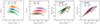 |
Fig. B.1. The effect of molecular abundance variations on optical depth and intensity. Left: Modeled CO optical depth as a function of CO intensity for xCO = 1.4 × 10⁻⁵ (green contours) xCO = 1.4 × 10⁻⁴ (blue contours) xCO = 1.4 × 10⁻³ (orange contours). Left center: Modeled HCN optical depth as a function of HCN intensity for xHCN = 10−9 (brown contours), xHCN = 10−8 (red contours), and xHCN = 10−7 (purple contours). Right center: Modeled HCN/CO intensity ratio as a function of CO optical depth for varying CO abundance. The HCN intensities are for xHCN = 10−8. Right: Modeled HCN/CO intensity ratio as a function of CO optical depth for varying HCN abundance. The CO intensities are for xCO = 1.4 × 10⁻⁴. Ten contours are drawn in even steps from the 16th to 100th percentile. Contours are shown in the right two panels for our sample of galaxies and the EMPIRE sample as the solid black and dashed black contours, respectively. |
We also find that increasing (decreasing) molecular abundance slightly increases (decreases) the median intensity (and, similarly, emissivity, see Eq. 1) in our models. We find ICO ≈ 63.0, 47.9, and 37.1 K km s−1 for xCO = 1.4 × 10⁻³, 1.4 × 10⁻⁴, and 1.4 × 10⁻⁵, respectively. HCN intensity appears to vary in roughly regular steps with molecular abundance (see Fig. B.1), with IHCN ≈ 8.9, 2.2, and 0.7 K km s−1 for xHCN = 10−7, 10−8, and 10−9, respectively. Furthermore, xHCN = 10−9 appears to produce HCN intensities that are also consistent with measurements from our sample (cf. Bemis & Wilson 2023) (relative to xHCN = 10−8), and some of the higher IHCN measurements of the EMPIRE sample (Jiménez-Donaire et al. 2019). As shown in Fig. B.1, there is a subsample of measurements with higher ICO that have HCN/CO ratios that fall below those produced by our models assuming xHCN = 10−8. It may be possible that these sources (which are mostly comprised of the more extreme systems in our sample) have a lower HCN abundance, on average. A higher HCN abundance (xHCN = 10−7) is likely not realistic for most molecular clouds (cf. Viti 2017), and also appears to produce higher HCN/CO ratios than what is measured in our sample and the EMPIRE sample.
In summary, the optical depth for xCO = 1.4 × 10⁻³ is ∼6 times larger than that for xCO = 1.4 × 10⁻⁴, but this makes little difference to the main conclusions of this paper as τCO > 10 and CO is in LTE for both of these values for the majority of our models, resulting in similar intensities and emissivities, and likewise similar results. For xCO = 1.4 × 10⁻⁵, the modeled CO ranges from only moderately optically thick to optically thin (log τ < 0). Since CO emission is likely optically thick in most molecular clouds, these results are not considered for analysis. We therefore focus on the results using the Solar CO abundance, xCO = 1.4 × 10⁻⁴, in the main text. We find that both xHCN = 10−8 and xHCN = 10−9 produce HCN intensities and HCN/CO ratios consistent with measurements in our sample and the EMPIRE sample. It is possible that the actual HCN abundances in the galaxies considered here vary between xHCN = 10−8 and xHCN = 10−9 (cf. Viti 2017). It is also possible that more extreme systems trend towards lower HCN abundance, but this is highly uncertain due to a lack of data of optically thin dense gas tracers. We therefore focus on the results of xHCN = 10−8 in the main text and we note that many of main conclusions would remain similar using a different value of xHCN, with slight offsets in HCN intensity and emissivity.
Appendix C: The impact of sensitivity limits
We re-derive emissivity from our models by excluding the low-density regions of our models that have HCN intensities below ∼0.1 K km s−1 (roughly the sensitivity limit in Tafalla et al. 2023) and show our results in Fig. C.1. We find that this has the effect of shifting αHCN to smaller values and more strongly impacts αHCN from the PHANGS-type models. This is because much of the emission in our PHANGS-type models resides at lower gas column densities. Additionally, the αHCN derived by Tafalla et al. (2023) appear more consistent with models in our sample that have larger gas surface density and larger velocity dispersion (i.e., the models based on measurements from the Antennae and NGC 3256 mergers). From Fig. 3. in Tafalla et al. (2023), we can see that the emission from their dense gas tracers appears to extend below their sensitivity limit, suggesting they are indeed missing some emission at low HCN intensity and low column density. Thus, this discrepancy could be because our models include emission from HCN arising from lower column densities below the detection limit of their study. As we find, this will disproportionately affect clouds with more emission at lower gas surface densities.
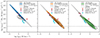 |
Fig. C.1. Inverse of the HCN emissivity (in units of the HCN conversion factor) as a function of HCN intensity. We plot the PHANGS-, NGC 4038/9-, and NGC 3256-type models from left to right as the blue, orange, and green filled contours. The black contours represent ⟨ϵHCN⟩−1 for the models where we make a cut at 0.1 K km s−1, which is analogous to a sensitivity limit in observations. For comparison, we also show the Gao & Solomon (2004a,b) value as the black, dotted horizontal line and several published values of αHCN from observations of Milky Way clouds (Dame & Lada 2023; Shimajiri et al. 2017). The gray, filled contour represents all models. We find the HCN emissivities from the PHANGS-type models to be most strongly impacted by a sensitivity cut. These models appear to have artificially lower ⟨ϵHCN⟩−1 (higher emissivity) as a result of the cut. |
All Figures
|
Fig. 1. Three models that are representative of clouds in (1) the PHANGS sample (NGC 2903), (2) NGC 4038/9, and (3) NGC 3256. Left: Example n–PDFs from our model parameter space assuming αPL = 3. Center: Temperature profiles of the example models. Right: Emissivity profiles of the example models. CO emissivity is shown as solid lines, and HCN emissivity is shown as dashed lines. The mass-weighted emissivity, ⟨ϵmol⟩, is given by Eq. (11). The range of densities over which radiative transfer is applied is slightly different between models, and depends on the average gas surface density of the model (see Sect. 2.3). We plot pn over a wider range of volume densities (left plot) than those used when performing radiative transfer (center and right plots). |
| In the text | |
|
Fig. 2. The model parameter space showing the range of gas velocity dispersions and gas surface densities considered in our analysis. The model points are plotted as gray points in the σv2/R − Σmol parameter space, and include a mix of cloud measurements from the PHANGS sample (Sun et al. 2020), NGC 4038/9 (Brunetti et al. 2024), and NGC 3256 (Brunetti et al. 2021). We also outline σv2/R − Σmol measurements of the Sun et al. (2020) PHANGS galaxies at 90 pc resolution (R = 45 pc, blue contours), NGC 4038/9 at 80 pc resolution (R = 40 pc, orange contours), and NGC 3256 at 80 pc resolution (R = 40 pc, green contours). The lower resolution data from Paper I are outlined by the black solid line. Example models from Fig. 1 are indicated in this plot as the blue (1), orange (2), and green (3) points. |
| In the text | |
|
Fig. 3. Modeled ICO and IHCN compared with the measured intensities of the Paper I sample (solid contours) and the EMPIRE sample (dashed contours Jiménez-Donaire et al. 2019). The blue filled contours are models whose Σ and σv are taken from the PHANGS sample (Sun et al. 2020), the orange filled contours are those taken from NGC 4038/9 (Brunetti et al. 2024), and the green filled contours are those taken from NGC 3256 (Brunetti et al. 2021). Ten contours are drawn in even steps from the 16–100th percentile. |
| In the text | |
|
Fig. 4. Correlations between modeled ICO (left two plots) and IHCN (right two plots) and their respective excitation temperatures and optical depths determined using Eqs. (13) and (14). The formatting is the same as in Fig. 3. We find that CO optical depth decreases with increasing ICO and CO excitation, in general agreement with the findings of previous studies (e.g., Bolatto et al. 2013; Narayanan et al. 2012; Narayanan & Krumholz 2014). In our models, HCN appears subthermally excited and moderately optically thick, also in agreement with the findings of previous studies (e.g., Dame & Lada 2023; Jiménez-Donaire et al. 2017). |
| In the text | |
|
Fig. 5. CO intensity (top row), the HCN intensity (center row), and HCN/CO ratio (bottom row) as a function of mean gas density, velocity dispersion, kinetic temperature, and gas column density. The column densities shown are from Eq. (12) for ICO and IHCN (top and center rows) and are the fiducial model column densities for the HCN/CO ratio (bottom row). The reference conversion factor values are shown in the intensity vs. column density plots as the dotted and dashed lines. We show the CO fits (top row) in the HCN plots (center row) as the gray dashed lines. Spearman rank coefficients are shown in the lower right corner. The formatting is the same as in Fig. 3. We plot fits from the results of the ALMOND survey (purple dotted line, Neumann et al. 2023) and Tafalla et al. (2023, red dashed line). Uncertainties on their respective fits are shown as the shaded areas. For comparison, we plot the results of Paper I sample (solid contours) and the EMPIRE sample (dashed contours, Jiménez-Donaire et al. 2019) in the HCN/CO ratio vs. gas surface density plot. Our models show strong positive correlations between the modeled line intensities and mean density, velocity dispersion, mean kinetic temperature, and gas column densities. IHCN appears to increase more rapidly with each of these parameters compared to ICO. The Spearman rank coefficients are shown in the lower right corner of each plot. |
| In the text | |
|
Fig. 6. 3.2 × IHCN/ICO as a function of the fraction of gas above (from left to right) n ∼ 102.5, 103.5, 104.5, and 105.5 cm−3. The formatting is the same as in Fig. 3. The fits are shown as the solid black line (see legend). The modeled IHCN/ICO scales most directly (has a slope closest to unity) with f(n > 103.5 cm−3), supporting previous findings that this line ratio is sensitive to gas above moderate densities. Although not shown here, the same is found when comparing the emissivity ratio, ⟨ϵHCN⟩/⟨ϵCO⟩, with the same gas fractions. The Spearman rank coefficients are shown in the lower right corner of each plot. |
| In the text | |
|
Fig. 7. The modeled emissivities of CO and HCN in units of M⊙ (K km s−1 pc2)−1 as a function of CO and HCN intensity, respectively. Left: Inverse of the CO emissivity (in units of the CO conversion factor) as a function of CO intensity, ⟨αCO⟩=⟨ϵCO⟩−1. We include the fit to our models (Eq. (17), solid line) and the 1σ uncertainty on the fit (gray shaded area). We also include the results of several numerical studies (Narayanan et al. 2012; Hu et al. 2022a; Gong et al. 2020, red dashed line, cyan dotted line, brown dash-dotted line, respectively) as well as the results of observational studies at ∼150 pc scales in the Antennae (pink dashed line, He et al. 2024) and PHANGS galaxies (purple dotted line, Teng et al. 2024). We note that we have recast the αCO − σv fit from Teng et al. (2024) in terms of ICO using the fit between ICO and σv from our models. Right: Inverse of the HCN emissivity (in units of the HCN conversion factor) as a function of HCN intensity, ⟨αHCN⟩=⟨ϵHCN⟩−1. We include a fit to our models (Eq. (18), solid line) and the 1σ uncertainty on the fit (gray shaded area). For comparison, we include several published values of αHCN from observations of Milky Way clouds (Dame & Lada 2023; Shimajiri et al. 2017), and we show the Gao & Solomon (2004a,b) value as the black dashed line. This figure demonstrates how well our models are able to reproduce previous numerical prescriptions of αCO, as well as observationally constrained values of αCO and αHCN. The formatting of the model output is the same as in Fig. 3. |
| In the text | |
|
Fig. 8. Ratio of the HCN and CO conversion factors (given in Eq. (19)) as a function of the ratio of the HCN and CO intensities, where we consider αHCN as a conversion factor for the total mass above n > 103.5 cm−3 (left) and n > 104.5 cm−3 (right). For comparison, we plot αHCN/αCO = 3.2 (solid black line), which is the ratio of the Gao & Solomon (2004a,b) conversion factor and Milky Way CO conversion factor. The formatting is the same as in Fig. 3. This figure demonstrates how emissivity is sensitive to the intensity per mass traced by a particular transition, whereas luminosity-to-mass conversion factors account for additional factors that allow us to estimate specific masses (e.g., total gas mass and dense gas mass) that may not be fully reflected in the molecular emissivity. We find that due to the subthermal excitation of HCN J = 1–0, this transition is a poor tracer of the of the gas mass above n > 104.5 cm−3 and is a better tracer of moderate gas densities (n > 103.5 cm−3), as found in previous observational studies. |
| In the text | |
|
Fig. 9. The relationships between modeled IHCN/ICO, f(n > 104.5 cm−3), fgrav, and tdep. Left: Modeled IHCN/ICO as a function of the gravitationally bound fraction of gas (fgrav) predicted by the LN+PL analytical models of star formation. Center: Fraction of dense gas above n > 104.5 cm−3 as a function of the gravitationally bound fraction of gas (fgrav) predicted by the LN+PL analytical models of star formation. The formatting is the same as in Fig. 3. The Spearman rank coefficients are shown in the lower right corner of the left and center panels. Right: Total gas depletion time (tdep) as a function of IHCN/ICO ratio. The models are shown as colored points. The measurements of tdep and IHCN/ICO from our sample of galaxies and the EMPIRE sample are shown as the solid black and dashed black contours, respectively. Our models find that the IHCN/ICO ratio is negatively correlated with fgrav as predicted by gravoturbulent models of star formation. Additionally, the fraction of dense gas above n > 104.5 cm−3 has an even steeper negative correlation with fgrav, as predicted by gravoturbulent models of star formation (e.g., Burkhart 2018; Burkhart & Mocz 2019). Thus, although IHCN/ICO is sensitive to gas above moderate densities, we conclude that a single molecular line ratio, such as HCN/CO, does not necessarily scale with the fraction of directly star-forming gas in clouds. We also find that models with the lowest estimates of fgrav and highest f(n > 104.5 cm−3) have the shortest depletion times, and the corresponding modeled IHCN/ICO and predicted depletion times are consistent with our data. |
| In the text | |
|
Fig. 10. Comparisons between theoretical predictions and our radiative transfer modeling of the relationships between ϵff, Pturb, tdep, and IHCN/ICO. Left: Model efficiency per free-fall time as a function of turbulent pressure shown three ways: (1) using modeled ICO and a fixed CO conversion factor for gas surface density estimates (colored points), (2) using the actual theoretical ϵff and Pturb values (red line), and (3) using modeled ICO with ⟨αCO⟩ = 1/⟨ϵCO⟩ (purple trend line). The shaded regions represent the full range of model scatter. Estimates of these quantities from our sample of galaxies and the EMPIRE sample are shown as the solid black and dashed black contours, respectively. Right: Model depletion time as a function of HCN/CO ratio shown three ways, using the same approach. We find that the scatter produced by variations in CO emissivity can account for a significant portion of the scatter seen in observations. Additionally, the trend in ϵff with Pturb is dependent on the assumed CO conversion factor. Pixel-by-pixel estimates of αCO may be necessary for accurate studies of star formation trends. We note that the offset in ϵff and tdep between methods (2) and (3) is a result of the modeled CO emission missing a fraction of the lower surface density gas in our models, to CO-dark gas. |
| In the text | |
|
Fig. 11. Comparisons between theoretical predictions and our radiative transfer modeling of the relationships between tdep, dense and IHCN/ICO. Left: Model dense gas depletion time as a function of HCN/CO ratio shown three ways: (1) using modeled IHCN and a fixed HCN conversion factor for gas surface density estimates (colored points), (2) using the theoretical depletion time of the fraction of gas above n > 103.5 cm−3 (red line), and (3) using modeled IHCN with ⟨αHCN⟩ = 3.2⟨αCO⟩ applied to estimate dense gas surface density (purple line). We also show the resulting trend using modeled IHCN with ⟨αHCN⟩ = 1/⟨ϵHCN⟩ (gray dashed line) for comparison. Right: Model dense gas depletion time plotted as a function of HCN/CO ratio shown three ways, this time overlaying depletion times of several fractions of gas: that above n > 102.5, 103.5, 104.5, 105.5, cm−3 (blue, red, green, and orange lines, respectively) as a function of the HCN/CO ratio. The shaded regions represent the full range of model scatter. We find that the HCN emissivity does not appear to contribute to the scatter of these relationships in the way that CO contributes to those in Fig. 10, which is likely due to the stronger dependence of HCN emissivity on excitation relative to optical depth. Additionally, the trend in dense gas depletion time with the HCN/CO ratio depends critically on the assumed HCN conversion factor. This figure also demonstrates that the HCN emissivity does not necessarily track the mass of star-forming gas (gray trend in the left panel), but that applying ⟨αHCN⟩ = 3.2⟨αCO⟩ to IHCN when estimating tdep, dense does a reasonable job at reproducing the depletion time of gas above moderate gas densities (red lines, both panels; see also Figs. 6 and 7 and Sect. 3.4). |
| In the text | |
|
Fig. B.1. The effect of molecular abundance variations on optical depth and intensity. Left: Modeled CO optical depth as a function of CO intensity for xCO = 1.4 × 10⁻⁵ (green contours) xCO = 1.4 × 10⁻⁴ (blue contours) xCO = 1.4 × 10⁻³ (orange contours). Left center: Modeled HCN optical depth as a function of HCN intensity for xHCN = 10−9 (brown contours), xHCN = 10−8 (red contours), and xHCN = 10−7 (purple contours). Right center: Modeled HCN/CO intensity ratio as a function of CO optical depth for varying CO abundance. The HCN intensities are for xHCN = 10−8. Right: Modeled HCN/CO intensity ratio as a function of CO optical depth for varying HCN abundance. The CO intensities are for xCO = 1.4 × 10⁻⁴. Ten contours are drawn in even steps from the 16th to 100th percentile. Contours are shown in the right two panels for our sample of galaxies and the EMPIRE sample as the solid black and dashed black contours, respectively. |
| In the text | |
|
Fig. C.1. Inverse of the HCN emissivity (in units of the HCN conversion factor) as a function of HCN intensity. We plot the PHANGS-, NGC 4038/9-, and NGC 3256-type models from left to right as the blue, orange, and green filled contours. The black contours represent ⟨ϵHCN⟩−1 for the models where we make a cut at 0.1 K km s−1, which is analogous to a sensitivity limit in observations. For comparison, we also show the Gao & Solomon (2004a,b) value as the black, dotted horizontal line and several published values of αHCN from observations of Milky Way clouds (Dame & Lada 2023; Shimajiri et al. 2017). The gray, filled contour represents all models. We find the HCN emissivities from the PHANGS-type models to be most strongly impacted by a sensitivity cut. These models appear to have artificially lower ⟨ϵHCN⟩−1 (higher emissivity) as a result of the cut. |
| In the text | |
Current usage metrics show cumulative count of Article Views (full-text article views including HTML views, PDF and ePub downloads, according to the available data) and Abstracts Views on Vision4Press platform.
Data correspond to usage on the plateform after 2015. The current usage metrics is available 48-96 hours after online publication and is updated daily on week days.
Initial download of the metrics may take a while.