| Issue |
A&A
Volume 691, November 2024
|
|
|---|---|---|
| Article Number | A121 | |
| Number of page(s) | 26 | |
| Section | Extragalactic astronomy | |
| DOI | https://doi.org/10.1051/0004-6361/202449496 | |
| Published online | 01 November 2024 | |
A 260 pc resolution ALMA map of HCN(1–0) in the galaxy NGC 4321
1
Argelander-Institut für Astronomie, Universität Bonn, Auf dem Hügel 71, 53121 Bonn, Germany
2
European Southern Observatory, Karl-Schwarzschild Straße 2, D-85748 Garching bei München, Germany
3
Department of Astronomy, The Ohio State University, 140 West 18th Ave, Columbus, OH 43210, USA
4
Observatorio Astronómico Nacional (IGN), C/ Alfonso XII, 3, E-28014 Madrid, Spain
5
Dept. of Physics, University of Alberta, Edmonton, Alberta T6G 2E1, Canada
6
LERMA, Observatoire de Paris, PSL Research University, CNRS, Sorbonne Universités, 75014 Paris, France
7
Universidad de Antofagasta, Centro de Astronomía, Avenida Angamos 601, Antofagasta 1270300, Chile
8
Max-Planck-Institut für Extraterrestrische Physik (MPE), Giessenbachstr. 1, D-85748 Garching, Germany
9
Institüt für Theoretische Astrophysik, Zentrum für Astronomie der Universität Heidelberg, Albert-Ueberle-Strasse 2, 69120 Heidelberg, Germany
10
Cosmic Origins Of Life (COOL) Research DAO, coolresearch.io
11
Department of Physics and Astronomy, University of Wyoming, Laramie, WY 82071, USA
12
National Radio Astronomy Observatory, 520 Edgemont Road, Charlottesville, VA 22903, USA
13
Research School of Astronomy and Astrophysics, Australian National University, Canberra, ACT 2611, Australia
14
ARC Centre of Excellence for All Sky Astrophysics in 3 Dimensions (ASTRO 3D), Australia
15
Visiting Fellow, Harvard-Smithsonian Center for Astrophysics, 60 Garden Street, Cambridge, MA 02138, USA
16
Astrophysics Research Institute, Liverpool John Moores University, 146 Brownlow Hill, Liverpool L3 5RF, UK
17
Max Planck Institute for Astronomy, Königstuhl 17, 69117 Heidelberg, Germany
18
Centro de Desarrollos Tecnológicos, Observatorio de Yebes (IGN), 19141 Yebes, Guadalajara, Spain
19
Sterrenkundig Observatorium, Universiteit Gent, Krijgslaan 281 S9, B-9000 Gent, Belgium
20
Department of Physics and Astronomy, Rutgers University, 136 Frelinghuysen Road, Piscataway, NJ 08854, USA
21
Department of Physics, Tamkang University, No.151, Yingzhuan Road, Tamsui District, New Taipei City 251301, Taiwan
22
National Astronomical Observatory of Japan, 2-21-1 Osawa, Mitaka, Tokyo 181-8588, Japan
23
Center for Astrophysics and Space Sciences, University of California, San Diego, 9500 Gilman Drive MC0424, La Jolla, CA 92093, USA
24
Sub-department of Astrophysics, Department of Physics, University of Oxford, Keble Road, Oxford OX1 3RH, UK
⋆ Corresponding author; lukas.neumann.astro@gmail.com
Received:
5
February
2024
Accepted:
13
June
2024
The property of star formation rate (SFR) is tightly connected to the amount of dense gas in molecular clouds. However, it is not fully understood how the relationship between dense molecular gas and star formation varies within galaxies and in different morphological environments. Most previous studies have typically been limited to kiloparsec-scale resolution such that different environments could not be resolved. In this work, we present new ALMA observations of HCN(1−0) at 260 pc scale to test how the amount of dense gas and its ability to form stars varies with environmental properties. Combined with existing CO(2−1) observations from ALMA and Hα from MUSE, we measured the HCN/CO line ratio, a proxy for the dense gas fraction, and SFR/HCN, a proxy for the star formation efficiency of the dense gas. We find a systematic > 1 dex increase (decreases) of HCN/CO (SFR/HCN) towards the centre of the galaxy, and roughly flat trends of these ratios (average variations < 0.3 dex) throughout the disc. While spiral arms, interarm regions, and bar ends show similar HCN/CO and SFR/HCN, on the bar, there is a significantly lower SFR/HCN at a similar HCN/CO. The strong environmental influence on dense gas and star formation in the centre of NGC 4321, suggests either that clouds couple strongly to the surrounding pressure or that HCN emission traces more of the bulk molecular gas that is less efficiently converted into stars. Across the disc, where the ISM pressure is typically low, SFR/HCN is more constant, indicating a decoupling of the clouds from their surrounding environment. The low SFR/HCN on the bar suggests that gas dynamics (e.g. shear and streaming motions) can have a large effect on the efficiency with which dense gas is converted into stars. In addition, we show that HCN/CO is a good predictor of the mean molecular gas surface density at 260 pc scales across environments and physical conditions.
Key words: ISM: molecules / galaxies: ISM / galaxies: individual: NGC 4321 / galaxies: star formation
© The Authors 2024
 Open Access article, published by EDP Sciences, under the terms of the Creative Commons Attribution License (https://creativecommons.org/licenses/by/4.0), which permits unrestricted use, distribution, and reproduction in any medium, provided the original work is properly cited.
This article is published in open access under the Subscribe to Open model. Subscribe to A&A to support open access publication.
1. Introduction
Galactic observations of dust in star-forming regions show that stars form in dense substructures, where the inferred star formation rate (SFR) is found to be linearly related to the amount of dense gas (e.g. Heiderman et al. 2010; Lada et al. 2010, 2012; Evans et al. 2014). Gao & Solomon (2004) found that this linear relation also holds for global measurements of galaxies when tracing the SFR with the total infrared (IR) luminosity and the dense gas mass (Mdense) via the luminosity of HCN(1–0). Molecular line emission from HCN has an effective critical density of neff ∼ 5 × 103 cm−3, which is at least one order of magnitude higher than that of CO (neff ≲ 102 cm−3; Shirley 2015). Over the past two decades, many studies have aimed at mapping HCN across other galaxies (e.g. Usero et al. 2015; Bigiel et al. 2016; Gallagher et al. 2018b; Jiménez-Donaire et al. 2019; Querejeta et al. 2019; Sánchez-García et al. 2022; Neumann et al. 2023b). The observations of star-forming spiral galaxies from these studies as well as numerical works (e.g. Onus et al. 2018) have reported that the IR luminosity tracing embedded SFR is tightly (scatter of ±0.4 dex) and linearly correlated with the HCN luminosity, tracing Mdense and spanning ten orders of magnitude (see e.g. Jiménez-Donaire et al. 2019; Neumann et al. 2023b; Bešlić et al. 2024; Schinnerer & Leroy 2024, for literature compilations) efficiency ( ).
).
Despite the clear relation between the SFR and the dense gas, there is still a total scatter of ≈1 dex that cannot solely be explained by the measurement uncertainties, instead indicating that the dense gas star formation efficiency (SFR/Mdense ≡ SFEdense) depends on other physical quantities. In the past decade, resolved kiloparsec-scale observations of nearby galaxies (e.g. Usero et al. 2015; Bigiel et al. 2016; Gallagher et al. 2018b,a; Jiménez-Donaire et al. 2019; Querejeta et al. 2019; Sánchez-García et al. 2022; Neumann et al. 2023b) have studied the variation of spectroscopic ratios, such as HCN/CO, a proxy of the dense gas fraction (fdense ≡ Mdense/Mmol, where Mmol is the molecular gas mass), and IR/HCN, a proxy of the dense gas star formation efficiency (SFEdense) with environmental properties, including the stellar mass surface density (Σ⋆), the molecular gas surface density (Σmol), and the hydrostatic pressure in the interstellar medium (ISM) disc (PDE). These studies find that fdense and SFEdense vary systematically with the environment. In particular, fdense is significantly enhanced, while SFEdense is systematically suppressed in high-surface density, high-pressure regions, indicating a connection between the properties of molecular clouds and their host environment. These results are also supported by studies of the Milky Way central molecular zone (CMZ), where SFEdense has been found to be systematically lower than across the Milky Way disc (e.g. Longmore et al. 2013; Kruijssen et al. 2014; Henshaw et al. 2023).
In their pioneering work, Gallagher et al. (2018a) found systematic correlations between the kiloparsec-scale fdense, SFEdense, and the molecular gas surface density measured at giant molecular cloud (GMC) scales (i.e. ∼100 pc). Building upon this, Neumann et al. (2023b) used HCN observations of 25 nearby galaxies from the ACA Large-sample Mapping Of Nearby galaxies in Dense gas (ALMOND) survey in order to compare the kiloparsec-scale spectroscopic line ratios with the properties of the molecular gas as traced by CO(2–1) on ∼100 pc scales from the Physics at High ANgular resolution GalaxieS–Atacama Large Millimetre Array (PHANGS–ALMA) survey (Leroy et al. 2021b). They showed that fdense increases and SFEdense decreases with increasing surface density (Σmol) and velocity dispersion (σmol) of the molecular gas measured at GMC scales. These results are also in agreement with predictions from models describing the star formation in turbulent clouds (e.g. Padoan & Nordlund 2002; Krumholz & McKee 2005; Krumholz & Thompson 2007) and the ISM disc structure (e.g. Ostriker et al. 2010), hence yielding a coherent picture between dense gas, star formation, and turbulent cloud models. In particular, these results have shown that SFEdense is not universal but depends on the environment and that density-sensitive line ratios such as HCN/CO are powerful extragalactic tools for tracing the underlying density structure at ∼100 pc scale even if measured at kiloparsec-scales.
Previous studies of the relationship between dense gas, star formation, and environment (e.g. Usero et al. 2015; Gallagher et al. 2018b,a; Jiménez-Donaire et al. 2019; Neumann et al. 2023b) were thus limited to mapping dense gas at kiloparsec-scales. There are only a few ∼100 pc resolution maps of HCN or other dense gas tracers (Kepley et al. 2014, M82, 200 pc; Chen et al. 2017, outer spiral arm of M51, 150 pc; Harada et al. 2018, NGC 3256, 200 pc; Viaene et al. 2018, GMCs in M31; 100 pc; Kepley et al. 2018, IC10, 34 pc; Querejeta et al. 2019, M51, 100 pc; Harada et al. 2019, circumnuclear ring of M83, 60 pc; Bešlić et al. 2021, NGC 3627, 100 pc; Martín et al. 2021, NGC 253, 250 pc with the potential of resolutions < 50 pc; Eibensteiner et al. 2022, central 2 kpc of NGC 6946, 150 pc; Sánchez-García et al. 2022, NGC 1068, 60 pc; Stuber et al. 2023, M51, 125 pc; Bešlić et al. 2024, NGC 253, 300 pc). However, these are typically less sensitive, and they target certain regions but not the full disc, in contrast to the observations presented here. Many of these works that mapped the whole molecular gas disc did not detect much emission in individual sight lines outside of galaxy centres, and hence the authors had to average over larger regions (e.g. via spectral stacking; Schruba et al. 2011; Caldú-Primo et al. 2013; Jiménez-Donaire et al. 2017, 2019; Neumann et al. 2023a) at the cost of spatial information. Apart from a few exceptions (M51, NGC 253; see references above), there are no deep wide-field studies of these dense gas ratios at sub-kiloparsec scales, which detect individual sight lines in different morphological environments across the whole molecular gas disc out to 10 kpc in galactocentric radius. Such a study is, however, needed in order to investigate the sub-kiloparsec structured ISM without blending many regions together that may have substantially different environmental and dynamical conditions for the formation of dense gas and its conversion to stars. A ≲500 pc scale resolution is needed in order to resolve environments such as the centre (size of ∼1 kpc), spiral arms (width of ∼1 kpc), and bar ends (size of ∼0.5 − 1 kpc).
In this work, we present new ALMA observations of dense molecular gas tracers, including HCN(1–0), HCO+(1–0), and CS(2–1), across the nearby spiral galaxy NGC 4321 at 3.5″ ∼ 260 pc resolution covering the full disc (i.e. out to 1.1 r25). These data are paired with CO(2–1) observations from PHANGS–ALMA (Leroy et al. 2021b), tracing the bulk molecular gas; extinction-corrected Hα from PHANGS–MUSE (Emsellem et al. 2022); 21 μm observations from PHANGS–JWST (Lee et al. 2023); and 33 GHz observations from VLA (Linden et al. 2020), which are used to trace the SFR. These observations give us one of the best high-resolution, high-sensitivity data sets combining interferometric and total power observations of high critical-density molecular line emission accompanied by the most robust tracers of SFR across the full disc of a nearby star-forming galaxy.
The paper is structured as follows. In Sect. 2, we present the observations and ancillary data of NGC 4321 used in this work, including new ALMA HCN observations. In Sect. 3, we describe the methods to derive the physical quantities from the observations, including the dense gas content, SFR, and ISM pressure. Then, in Sect. 4, we show the results, and we analyse the dense gas spectroscopic line ratios and their variation with environment, which are discussed in Sect. 5. Finally, we conclude and summarise the key findings in Sect. 6.
2. Observations
2.1. The target – NGC 4321
We selected NGC 4321 for this study as previous ALMA/IRAM mapping showed clear HCN detections, supporting data covers almost all aspects of the ISM and galactic structure, and its favourable distance to obtain a wide area map while still resolving, for example, the galactic centre, bar, arms, and other regions. NGC 4321 (main properties listed in Table 1) is a well-studied, spiral, barred (Querejeta et al. 2021) galaxy (Hubble classification: SABbc) that contains a large reservoir of molecular gas (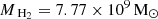 ; Leroy et al. 2021b), is actively forming stars (
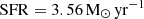 ; Leroy et al. 2019) and can be observed relatively face-on (i = 38.5°; Lang et al. 2020). Fig. 1 shows a James Webb Space Telescope (JWST) three-colour image overlaid with HCN contours from this work that highlight the spiral arm structure of the galaxy, seen in dust, gas and star formation. At a distance of d = 15.2 Mpc (Anand et al. 2021) it is relatively nearby, allowing access to GMC scales (< 100 pc) at ∼1″ angular resolution. Moreover, NGC 4321 is a spiral galaxy with similar stellar mass (
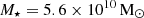 ) to our Galaxy (
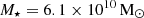 , Licquia & Newman 2015), making it an interesting object to compare with Galactic studies. NGC 4321 has been extensively studied as part of large observing campaigns like PHANGS–ALMA (Leroy et al. 2021b), mapping CO(2–1) across the full disc of the galaxy at ∼1″ ∼ 100 pc resolution, as well as the Eight Mixing Receiver (EMIR) Multiline Probe of the ISM Regulating Galaxy Evolution (EMPIRE; Jiménez-Donaire et al. 2019) and ALMOND (Neumann et al. 2023b) surveys, mapping various dense gas tracers including HCN and HCO+ with the IRAM 30-m telescope and the Atacama Compact Array (ACA), respectively, at kiloparsec scales. Furthermore, NGC 4321 was part of the ALMA science verification CO(1–0) observations (Pan & Kuno 2017) and has high-quality maps of H I (HERACLES; Leroy et al. 2009), stellar structure (S4G; Sheth et al. 2010), star formation tracers (Hα from MUSE; Emsellem et al. 2022), as well as near and mid-infrared maps from the JWST (Lee et al. 2023). We show a compilation of the key observations used in this work in Figure 2.
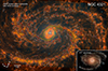 |
Fig. 1. JWST three-colour image of NGC 4321 overlaid with HCN contours. The background image is a three-colour composite using the MIRI and NIRCAM instruments observations (red = F770W + F1000W + F1130W + F2100W, green = F360M + F770W, and blue = F300M + F335M) taken from the PHANGS–JWST treasury survey (Lee et al. 2023). Overlaid HCN(1–0) contours (new data presented in this work), tracing the dense molecular gas are drawn at S/N levels of (2, 3, 5, 10, 20, 30, 50, 100). The sites of star formation (reddish hues) appear spatially well correlated with the dense gas traced by HCN. This image is rotated by 21° with respect to the right ascension-declination plane as indicated by the north (N)-east (E) coordinate axes in the bottom left. The bottom right image shows a rgb image (red = F814W, green = F555W, blue = F438W + F336W + F275W) from PHANGS–HST (Lee et al. 2022). |
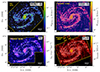 |
Fig. 2. NGC 4321 data used in this study, each at the native resolution of the respective observations indicated in the bottom left of each panel. Top left: HCN(1–0) moment-zero map presented in this work. Top right: CO(2–1) moment-zero map from PHANGS–ALMA (Leroy et al. 2021b). Bottom left: Extinction-corrected Hα flux density from PHANGS–MUSE (Emsellem et al. 2022). Bottom right: 21 μm flux density from MIRI-F2100W (PHANGS–JWST; Lee et al. 2023). In each panel, white-to-black-gradient contours show HCN moment-zero signal-to-noise ratio levels of (2, 3, 5, 10, 20, 30, 50, 100) as in Fig. 1. The yellow-coloured outline shows the FOV of the respective observations. |
Properties of NGC 4321.
2.2. New ALMA maps of HCN
In this work, we present ALMA Band-3 observations (2017.1.00815.S; PI.: Molly Gallagher) that mapped HCN(1–0) (along with HCO+(1–0) and CS(2–1)) across the full disc of the galaxy NGC 4321 at a high angular resolution of 3.5″ using 216.7 h of ALMA telescope time. The observations combine interferometric observations from the 12-m array (18.1 h observing time) with the ACA consisting of the 7-m array (73.4 h) and the 12-m dishes observing in total power (TP) mode (125.2 h). The mapped area on the sky is 200″ × 120″ large created via a mosaic consisting of 27 Nyquist-spaced pointings with the 12-m array. The spectral setup encompasses four spectral windows, each with a bandwidth of 1875 MHz and a channel width of 976 kHz. The first window, centred at 88.5 GHz targets HCN(1–0) (88.6 GHz) and HCO+(1–0) (89.2 GHz). The second window at 87.0 GHz covers SiO(2–1) (86.9 GHz) and isotopologues of HCN and HCO+, that is, H13CN (1–0), H13CO+ (1–0). The third spectral window at 98.5 GHz comprises CS(2–1) (97.9809533 GHz). The fourth spectral window at 100 GHz is used to detect continuum emission. The channel width of ≈3 km s−1 is sufficient to resolve the spectral lines across the whole disc of the galaxy, and the bandwidth of ≈6000 km s−1 allows for mapping of all the lines over the full velocity extent.
The data reduction was performed using the PHANGS–ALMA pipeline (details can be found in Leroy et al. 2021a), which utilises the standard ALMA data reduction package CASA (CASA Team 2022). In this first study, we focus on HCN(1–0) (hereafter HCN) as the brightest proxy for dense molecular gas. The resulting HCN position-position-velocity cube has ∼8 mK noise per 5 km s−1 channel. The high resolution, which corresponds to 260 pc physical scales, allowed us to resolve individual environmental regions, including the centre, bar, bar ends, spiral arms, and interarm regions (Fig. 3, right panel), yielding detection of 302 independent lines of sight in HCN emission (see Sect. 3.1 for details on masking and derivation of moment-zero maps).
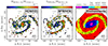 |
Fig. 3. NGC 4321 maps sampled at beam size. Left: HCN/CO line ratio map, as a proxy of the dense gas fraction (fdense). The CO(2–1) data are taken from the PHANGS-ALMA survey (Leroy et al. 2021b). Middle: SFR surface density-to-HCN line intensity ratio, as a proxy of the dense gas star formation efficiency (SFEdense). The SFR surface densities are obtained from the Balmer decrement-corrected Hα flux computed from PHANGS-MUSE data (Emsellem et al. 2022; Belfiore et al. 2023). Black contours show HCN S/N levels of 3, 10, 30, 100, and 300, in each of the panels. In the left and middle plots, only pixels above 1-sigma are shown. The colour scale goes from the 10th to the 95th percentile of pixels above 1-sigma noise level. Right: Environmental region mask from Querejeta et al. (2021), which is created based on the Spitzer 3.6 μm maps tracing the stellar mass content. Here, we select the regions centre, bar, bar ends, spiral arms and interarm, where the interarm includes the interbar region. The dotted ellipses show loci of constant galactocentric radius (rgal), drawn at rgal = 2.6 kpc and rgal = 9.17 kpc, where the latter indicates the largest radius completely covered by the HCN field of view. |
2.3. Ancillary data
In addition to the new HCN data, tracing dense molecular gas, we use CO observations to trace the bulk molecular gas (Sect. 3.2) and Hα observations to trace SFR (Sect. 3.4). Furthermore, we include H I 21-cm observations (Appendix A.2) and 3.6 μm infrared maps (Appendix A.3) to trace the atomic gas and the stellar mass content, respectively. In the Appendix, we further present additional tracers of the SFR, that is, F2100W hot dust observations from JWST (Appendix C.1) and 33 GHz free-free emission from the VLA (Appendix C.2), supporting the use of Hα as the primary SFR tracer in this work.
3. Methods
3.1. Integrated intensity maps
We produce integrated intensity maps (moment-zero maps) from the CO and HCN position-position-velocity (PPV) cubes following Neumann et al. (2023b). The methodology goes back to Schruba et al. (2011) and was utilised in several studies such as EMPIRE (Jiménez-Donaire et al. 2019), CO isotopologue Line Atlas within the Whirlpool galaxy Survey (CLAWS; den Brok et al. 2022) and ALMOND (Neumann et al. 2023b). First, we homogenise the data by convolving the CO data to the HCN resolution (using convolution.convolve from astropy). Then, we adopt a hexagonal spaxel grid with a beam-size spaxel separation and sample all data to the same spaxel grid and spectral axis. This means that every hexagonal pixel is an independent line-of-sight (LOS) measurement. Then, we create velocity masks based on the CO on a pixel-by-pixel basis to select the velocity range where we also expect to find HCN emission. This is done by building a 4σ mask that is expanded into channels above 2σ in order to recover broader emission belonging to a 4σ core (see e.g. Neumann et al. 2023b, for more details about the masking). By applying the CO-based mask to our data, we compute the integrated intensity of CO (WCO) and HCN (WHCN) by integrating the line’s brightness temperatures (Tline, where line = {CO, HCN}) over the velocity range selected by the mask
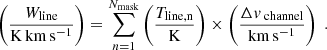
The uncertainties of the integrated intensities (σWline) are then given by
where σTline is the standard deviation in the emission-free channels (i.e. channels not selected by the mask), Δvchannel is the channel width of 5 km s−1 and Nmask is the number of channels selected by the mask for each LOS.
We note that we also homogenised the two-dimensional maps, for example, the MUSE Hα and JWST 21 μm maps, with the produced moment-zero maps. This means, we convolve the maps to the 260 pc HCN resolution and reproject them onto the same beam-size hexagonal pixel grid. A summary of the data products is presented in Fig. E.3. We describe the derivation of the physical quantities in the following subsections.
3.2. Molecular gas surface density – CO
We use CO(2–1) (hereafter CO) line observations from PHANGS–ALMA (Leroy et al. 2021b) to trace the bulk molecular gas. For NGC 4321, the CO data are at 1.67″ resolution, which corresponds to 120 pc physical scale at the distance of the galaxy1. We infer the molecular gas surface density (Σmol) from the CO(2–1) line intensity (WCO(2–1)) using the CO(2–1)-to-CO(1–0) line ratio (R21) and the CO-to-H2 conversion factor (αCO), which includes the mass contribution from helium:

cos(i) corrects for the inclination i = 38.5° of the galaxy. Throughout this work, we adopt two methods (see Appendix A.1 for more details): 1) using constant αCO and R21 conversion factors (Appendix A.1.1) that enter the estimation of the dense gas fraction as traced by the HCN-to-CO line ratio (Sect. 3.3). We use a constant αCO for the HCN-to-CO line ratio due to the poor knowledge about variations of the HCN-to-dense gas conversion factor thus keeping fdense proportional to HCN/CO. 2) using spatially varying αCO and R21 (Appendix A.1.1) for computing Σmol and the dynamical equilibrium pressure (Sect 3.6).
3.3. Dense gas fraction – HCN/CO
In this study, we present new HCN observations (Sect. 2.2) and use the HCN line intensity (WHCN) as a proxy for the amount of dense gas. For the main part of this work, we focus on studying the observational HCN-to-CO line ratio, that is, WHCN/WCO(2–1) (hereafter HCN/CO(2–1) or simply HCN/CO) as a density-sensitive line ratio. Gallagher et al. (2018a) and Neumann et al. (2023b) have shown that HCN/CO is indeed tracing the ∼100 pc-scale mean gas density and it has been reported to scale with the gas surface density within galactic clouds (Tafalla et al. 2023) as expected by molecular line modelling (Leroy et al. 2017). In addition, the reported linear relation between the HCN/CO and N2H+/CO line ratios across galactic and extragalactic studies underlines the credibility of HCN/CO as a proxy for the dense gas fraction (Jiménez-Donaire et al. 2023; Stuber et al. 2023). Throughout the discussion (Sect. 5), we comment on the implications of the dense gas fraction (fdense) as a physical quantity proportional to HCN/CO with some uncertainties linked to abundance, temperature and opacity.
Following many previous works (e.g. Usero et al. 2015; Bigiel et al. 2016; Gallagher et al. 2018b,a; Jiménez-Donaire et al. 2019; Bemis & Wilson 2019; Neumann et al. 2023b), the dense gas fraction is defined as the ratio of the dense gas to bulk molecular gas surface density (fdense = Σdense/Σmol):
The above conversion adopts constant mass-to-light ratios  (Bolatto et al. 2013) and
  (Onus et al. 2018) for CO and HCN, respectively, and a fiducial CO(2–1)-to-CO(1–0) line ratio of R21 = 0.65 (den Brok et al. 2022; Leroy et al. 2022). Here, we use the above conversion to infer fdense as an alternative axis in the HCN/CO relations.
The adopted constant HCN-to-dense gas mass conversion factor is expected to trace gas above nH2 ≈ 5 × 103 cm−3 (Onus et al. 2018)2. In contrast to αCO, systematic variations of αHCN are poorly understood and estimated values range from 0.3 to  , spanning three orders of magnitude (García-Burillo et al. 2012; Kauffmann et al. 2017; Nguyen-Luong et al. 2017; Shimajiri et al. 2017; Evans et al. 2020; Barnes et al. 2020; Tafalla et al. 2023), where extragalactic studies, capturing larger physical areas and thus more diffuse emission typically yield values around
  to
to  . The αHCN conversion factor might vary similarly to αCO due to its dependence on optical depth, which is a key driver of αCO variations (Teng et al. 2023), though HCN and CO optical depth variations are not expected to be identical. In that case, we could even induce systematic trends by adopting a more accurate, spatially varying αCO, but keeping αHCN constant. Therefore, the best current approach is to study the observational HCN/CO line ratio.
As laid out in this section, we adopt the classical view of utilising HCN/CO as a proxy of fdense. However, we want to point out that the conversion factors are subject to large uncertainties (especially αHCN) such that our fdense estimates are expected to be uncertain by a factor of a few. Therefore, recent works (e.g. Gallagher et al. 2018b,a; Jiménez-Donaire et al. 2019; Neumann et al. 2023b; Tafalla et al. 2023), which study HCN/CO as a function of the molecular gas surface density suggest to interpret HCN/CO as a predictor of the cloud-scale (∼100 pc) average gas density based on the robust relation between HCN/CO and Σmol (see also Sect. 4.5). This means, HCN/CO is expected to track ⟨Σmol⟩ more robustly than fdense. We note, that in turbulent cloud models (Krumholz & McKee 2005), an increase of HCN/CO would indicate an increase in fdense as well as ⟨Σmol⟩. Therefore, both interpretations (i.e. HCN/CO traces fdense and HCN/CO traces ⟨Σmol⟩) are reasonable. Throughout this work, we base our results on the observable HCN/CO line ratio, and provide a secondary fdense-axis so that, taking into considering aforementioned caveats, HCN/CO can be interpreted as the dense gas fraction via a proportional conversion or alternatively as an indicator of the mean gas density.
3.4. Star formation rate – Hα
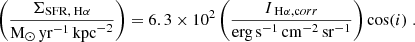
We use Hα recombination line emission taken by the Multi Unit Spectroscopic Explorer (MUSE) of the Very Large Telescope (VLT) as part of the PHANGS–MUSE survey (Emsellem et al. 2022) to trace the SFR. In Appendix C, we discuss using alternative SFR tracers including 21 μm (F2100W) hot dust emission from JWST (Lee et al. 2023) and 33 GHz free-free emission from the VLA (Linden et al. 2020), which can differ significantly (up to one order of magnitude) in the central few kiloparsecs of galaxies. Here, we find that SFR values inferred from the 33 GHz emission confirm the extinction-corrected Hα inferred values in the centre of NGC 4321. Moreover, 21 μm emission also yields similar SFR values (within 0.2 dex) when adopting a linear conversion (for more details see Appendix C.3). Therefore, throughout this work we adopt Hα emission as a robust tracer of SFR validated by free-free data in the centre.
We used the Balmer decrement-corrected Hα maps to measure the SFR surface density (ΣSFR). Those rely on the extinction curve from O’Donnell (1994) as described in Pessa et al. (2022) and Belfiore et al. (2023). The attenuation corrected Hα flux (LHα, corr) is converted into SFR via  using the conversion factor CHα = 5.3 × 10−42 from Calzetti et al. (2007). This conversion assumes a constant star formation history, age of 100 Myr, solar metallicity, and a Kroupa (2001) initial mass function (IMF) (for more detail on the SFR calibration, see Belfiore et al. 2023). In surface density units the above formalism translates to
3.5. Dense gas star formation efficiency – SFR/HCN
We took the ratio of the SFR surface density (ΣSFR) to the HCN line intensity (WHCN), that is, ΣSFR/WHCN (hereafter SFR/HCN), as a proxy of the star formation efficiency of the dense gas (SFEdense). Similar to HCN/CO tracing fdense, we also focus on the more observationally based SFR/HCN in our analysis and discuss implications on the inferred SFEdense connected to uncertainties in the conversion factor (αHCN). SFEdense is defined as the ratio of SFR surface density to dense gas mass surface density (SFEdense = ΣSFR/Σdense) as in previous works (listed in Sect. 3.3):
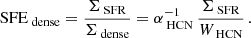
The above equation yields
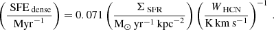
when using the same, constant HCN-to-dense gas mass conversion ( , Onus et al. 2018) as for fdense (Sect. 3.3).
3.6. Dynamical equilibrium pressure
We compute the dynamical equilibrium pressure, or ISM pressure (PDE) at 260 pc scale following the prescription by Sun et al. (2020). In this prescription the dynamical equilibrium pressure is composed of a pressure term created by the ISM due to the self-gravity of the ISM disc and a term due to the gravity of the stars (see e.g. Spitzer 1942), such that
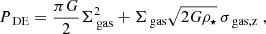
where we assumed a smooth, single-fluid gas disc and that all gas shares a similar velocity dispersion so that Σgas = Σmol + Σatom is the total gas surface density, composed of a molecular (Σmol) and an atomic (Σatom) gas component. ρ⋆ is the stellar mass volume density (Appendix A.3) near the disc mid-plane and σgas,z is the velocity dispersion of the gas perpendicular to the disc.
In many previous extragalactic studies (e.g. Spitzer 1942; Elmegreen 1989; Elmegreen & Parravano 1994; Wong & Blitz 2002; Blitz & Rosolowsky 2004, 2006; Leroy et al. 2008; Koyama & Ostriker 2009; Ostriker et al. 2010; Ostriker & Shetty 2011; Kim et al. 2011; Shetty & Ostriker 2012; Kim et al. 2013; Kim & Ostriker 2015; Benincasa et al. 2016; Herrera-Camus et al. 2017; Gallagher et al. 2018a; Fisher et al. 2019; Schruba et al. 2019; Jiménez-Donaire et al. 2019) PDE was typically estimated using Eq. (8) with homogenised Σgas, ρ⋆, σgas,z at kiloparsec scales. Recently, Sun et al. (2020) came up with a new formalism that makes use of the high resolution ∼100 pc scale CO(2–1) data from PHANGS–ALMA. Most importantly, it takes into account the self-gravity of the (molecular) gas at high resolution. In this study we adopt their formalism and combine the 120 pc scale molecular gas term (⟨Pcloud⟩; converted to the lower resolution via a Σmol-weighted average) with the 260 pc scale atomic gas term (Patom):

⟨Pcloud⟩ consists of three terms accounting for the self-gravity of the molecular gas, the gravity of larger molecular structures and the gravity of stars. Patom includes the self-gravity of the atomic gas and the gravitational interaction of the atomic gas with the 260 pc scale molecular gas and the stars (see Appendix A.4 for more details).
3.7. Morphological environmental masks
We adopt the environmental masks presented in Querejeta et al. (2021), which identify morphological environmental regions based on the appearance of the stellar mass content traced by the Spitzer 3.6 μm emission from S4G (Sheth et al. 2010). We use the “simple” mask, where each pixel is uniquely assigned to a dominant environment. We define the bar ends as the overlap of the spiral arms with the bar footprint. For simplicity, we combine interbar, interarm into one region, referred to as interarm. We end up with five environments – centre, bar, bar ends, spiral arms, interam, which are re-sampled onto the same hexagonal grid as the other data defined by the HCN map (Sect. 3.1). We show the adopted environments in the right panel of Fig. 3.
Line intensities and luminosities by environment.
3.8. Stacking and linear regression
To study the average trends, we stack the data (HCN, CO, SFR) in equally spaced bins in linear scale (rgal) or logarithmic scale (PDE). The spectral stacking is done using the python package PyStacker3, which yields average CO and HCN spectra in each respective bin (the stacked spectra are presented in Fig. 4 and in Appendix B). Those average spectra are used to compute the average integrated intensities in each bin. For SFR, we simply compute the mean of the SFR values in the respective bin. The bin ratios are then computed as the ratios of the stacked measurements. To first order, HCN and CO lines show similar kinematics across most of the galaxy, so the line ratio, which we discuss in this first paper, encodes most of the relevant information.
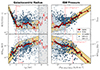 |
Fig. 4. Stacked spectra by environment. The CO(2–1) line (red) is used to correct for the effect of the velocity field. In every panel, the HCN(1–0) intensities are multiplied by a factor of 30 for better comparison with the CO intensities. The grey-shaded area indicates the velocity window over which the integrated intensities are computed. |
We fit the stacked data in order to probe the underlying global relation without “population” biases and to not be dominated by non-detections in constraining the best-fit line. We note, however, that we have also fitted the individual sightline measurements using LinMix4, resulting in similar fit relations in agreement within 1-sigma uncertainties with the fits reported here for the binned data. We use these sightline fits to quantify the uncertainty of the regression slopes since the piecewise fitting routine (see below) does not yield uncertainties.
We then apply a multivariate adaptive regression spline (MARS; Friedman 1991) model to the binned data in order to find the best piecewise linear regression function that describes the data (see Sect. 4.2 and 4.3). MARS is a generalisation of a recursive partitioning algorithm, which iteratively splits the data into separate x-axis regimes and optimises the split point with respect to the piecewise linear regression in each regime via minimising the χ2 value of the data to the model. The algorithm is adapted to only add another split point if a further component significantly improves the fit, meaning that the χ2 value is improved by more than 0.01. In this way, we employ a statistically robust and objective method to find the threshold at which the trends change significantly thus identifying physically different regimes in the relations. To perform the MARS model we utilise the R-package earth5. Here, we force the model to only consist of up to two linear functions, that is, it can either find one or two regimes depending on if a second regime improves the fit significantly.
HCN/CO and SFR/HCN statistics by environment.
4. Results
4.1. Dense gas spectroscopic ratios across the full disc of NGC 4321 at 260 pc scale
The new high-resolution deep wide-field HCN observations presented in this work allowed us for the first time to study variations of HCN/CO, a proxy of fdense, and SFR/HCN, a proxy of SFEdense, across the full disc of a Milky Way-like galaxy at unprecedented resolution (260 pc) such that morphological environments could be well separated. These data represent one of the rare deep wide-field HCN maps of a nearby galaxy that allows analysis of 275 detected sight lines even outside of the galaxy centre, as illustrated by Fig. 2 (top left panel). By environment, we detected 42 HCN sight lines in the centre, 70 in the bar, 26 in the bar ends, 97 in the spiral arms, and 40 in the interarm regions (we list the values along with stacked integrated intensities and luminosities in Table 2). Figure 2 shows that where CO was detected; HCN is also often detected, though we found HCN to be more concentrated in the centre, bar, bar ends, and spiral arms. To first order, Hα and 21 μm emission, tracers of SFR, are spatially correlated with both CO and HCN. The 260 pc scale resolved observations of NGC 4321 confirm the well-established linear correlation between HCN luminosity and SFR.
In Figure 3, we show maps of HCN/CO and SFR/HCN. The variability of these ratios provides information about how HCN correlates with CO and SFR, as discussed below. In the following, we distinguish between five environmental regions (centre, bar, bar ends, spiral arms, interarm) introduced in Sect. 3.7. The right panel of Figure 3 shows the applied environments sampled onto the same coordinate grid and overlaid with HCN contours. Overall, the HCN emission follows the stellar mass morphology such that outside of the centre, most of the HCN emission is associated with the stellar spiral arms, whereas less HCN is found in the interarm regions. However, there is also large amounts of (dense) molecular gas when following the bar eastward beyond the bar ends. These regions, here depicted as interarm regions, could be interpreted as minor spiral arms or spurs between the spiral arms that harbour large amounts of molecular gas (similar to the spurs observed in M51; Schinnerer et al. 2017). Though not explored here and considered part of the interarm environment, it could be interesting to study these spurs in more detail in further studies.
4.1.1. HCN/CO variations
Figure 5 (left panel) shows the distribution of HCN/CO values in different environments, stacked in increments of 0.1 dex. We also show the mean and scatter of the detected data of the respective distributions. Since S/N clipping systematically selects luminous HCN regions, these values will be biased towards high HCN/CO and low SFR/HCN, with the significance of the bias depending on the completeness of detections in the respective environments. Therefore, we also show the stacked means of all sight lines across each environment (squares in Fig. 5). The values are listed in Table 3.
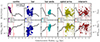 |
Fig. 5. Violin plots of dense gas spectroscopic ratios separated by environmental regions. Left: HCN/CO line ratio, a proxy of the dense gas fraction, fdense. Right: SFRHα/HCN, a proxy of the dense gas star formation efficiency, SFEdense, in units of |

We find that HCN/CO spans roughly 0.6 dex when considering only detected lines of sight (S/N ≥ 3). In agreement with previous studies (e.g. Usero et al. 2015; Bigiel et al. 2016; Gallagher et al. 2018b; Jiménez-Donaire et al. 2019; Querejeta et al. 2019; Neumann et al. 2023b; Bešlić et al. 2024), HCN/CO increases towards the centre of the galaxy, where it reaches values around 0.1 (mean of 0.089 ± 0.0003), indicating an increase of the dense gas fraction or average gas density in centres of galaxy or/and a change in excitation conditions, for example, optical depth, gas temperature, or abundance (e.g. Jiménez-Donaire et al. 2017; Eibensteiner et al. 2022).
Throughout the disc of the galaxy (spiral arms and interarm region), HCN/CO is lower by a factors of two (mean of ≤0.049 across detections, with 1-sigma scatter of ±0.15 dex) compared to the centre (mean of 0.89) and does not show trends with radius or environment (further discussed in Sect. 4.2). This suggests, assuming that HCN/CO is a robust tracer of density (Neumann et al. 2023b), that the density distribution of the molecular gas, which is detected in HCN, is very similar across the disc of NGC 4321. However, we note that when taking into account censored data, the average HCN/CO is lower by almost a factor of two in the interarm region (mean of 0.015 ± 0.003) than in the spiral arms (mean of 0.028 ± 0.001).
Compared to the disc of the galaxy and taking into account non-detections, we observed enhanced HCN/CO in the bar ends (mean of 0.043 ± 0.001) pointing towards the piling up of dense molecular gas, for example, via gas streams from the spiral arms and the bar towards the bar ends (predicted by simulations e.g. Renaud et al. 2015 and observed in NGC 3627 Bešlić et al. 2021). Moreover, we observe indications of a mild gradient of HCN/CO with angular offset from the spiral arm across the southern spiral arm (Fig. 3). If taken at face value, the found HCN/CO gradient could imply a systematic density variation across the spiral arm, changing the physical conditions of the emitting gas.
4.1.2. SFR/HCN variations
Analogously to HCN/CO, we show violin plots along with mean scatter bars of SFR/HCN, a proxy of SFEdense, in the right panel of Figure 5. In total, the SFR/HCN values span about 2 dex across the detected LOSs indicating a large scatter in SFR/HCN, consistent with the cloud-to-cloud variation found in galactic studies (e.g. Moore et al. 2012; Eden et al. 2012; Csengeri et al. 2016; Urquhart et al. 2021). Certainly, some of the scatter can be attributed to systematic variations with molecular gas conditions (e.g. Neumann et al. 2023b) and environment (discussed in this work).
In the inner ∼4 kpc of NGC 4321, SFR/HCN appears to be spatially anti-correlated with HCN/CO (Fig. 3), confirming kiloparsec-scale measurements of previous studies, for example, Usero et al. (2015), Gallagher et al. (2018b), Jiménez-Donaire et al. (2019). As has been reported in several previous studies (e.g. Chen et al. 2015; Bešlić et al. 2021; Neumann et al. 2023b), SFR/HCN decreases towards the centre of the galaxy (mean of 0.025 ± 0.0001 in units of  ) supporting the picture that HCN traces more of the bulk material in dense environments. In addition to the centre, we find SFR/HCN to be particularly low in the bar of the galaxy (mean of 0.039 ± 0.001) (further discussed in Sect. 5.3), while it is higher by a factor of two to seven across the disc (i.e. bar ends, spiral arms and interarm regions, have means between 0.086 ± 0.003 and 0.274 ± 0.057).
The low SFR/HCN in the centre and bar environments can be explained in several ways. On the one hand, the low SFR/HCN can be caused by an increase in HCN emissivity. On the other hand, it could indicate a decrease in SFR at fixed HCN emission, that is, an actually reduced star formation efficiency of dense gas. Another alternative explanation put forward in previous works (e.g. Gallagher et al. 2018b; Jiménez-Donaire et al. 2019; Neumann et al. 2023b) is that, in these high-density, high-pressure environments, HCN is not tracing the actual overdensities anymore, but become more of a bulk molecular gas tracer. The former can be caused by radiative trapping (Shirley 2015; Jiménez-Donaire et al. 2017), lowering the effective critical density of HCN and yielding subthermally excited HCN emission (Leroy et al. 2017; Jones et al. 2023; García-Rodríguez et al. 2023) or electron excitation (Goldsmith & Kauffmann 2017) boosting the HCN emission. The reduced SFEdense could be the result of a strong influence of gas dynamics on the star-formation process (bar), for example, shear, hampering the formation of stars despite the availability of dense gas (Sect. 5.3). We note that centres are much more affected by variations in conversion factors (αCO and αHCN) than discs, and the SFR estimator (extinction-corrected Hα) is potentially less accurate due to increasing dust attenuation towards centres and the effects of AGN-driven Hα emission (although this galaxy has no AGN according to Véron-Cetty & Véron 2010). Most probably, the low SFR/HCN in the centre is a combination of an increase in gas turbulence driving HCN emission and a lower HCN-to-dense gas conversion factor.
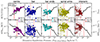 |
Fig. 6. Dense gas spectroscopic ratios as a function of galactocentric radius and environmental pressure. Top: HCN/CO, a proxy of the dense gas fraction, fdense, as a function of rgal and ⟨PDE⟩. Bottom: SFR/HCN, a proxy of the dense gas star formation efficiency, SFEdense, against rgal and ⟨PDE⟩. Significant data, that is, S/N ≥ 3, are shown as blue markers. Low significance data (S/N < 3) are shown in light blue. The red hexagon markers denote significant spectral stacks taken over all data, with the bars showing the uncertainties obtained from the stacked spectra. The red arrows indicate 3σ upper limits of the HCN stacks resulting in HCN/CO upper limits and SFR/HCN lower limits. In the left panels, the hatched region (rgal > 9.17 kpc) indicates the range where the map is not complete (compare with Fig. 3). The vertical red dashed lines indicate the x-axis values separating two regions with different linear regression behaviour based on the MARS model. The dashed black lines indicate the best-fit lines resulting from the MARS model (Table 4). The gold-shaded area shows the 3-sigma scatter of the detected sightlines about the fit line. |
Spiral arms, interarm regions and bar ends share a similar SFR/HCN distribution suggesting they are similarly efficiently converting dense gas into stars. This is contradictory to the hypothesis that bar ends are the sites of increased star formation efficiency, for example, via cloud-cloud collision that might boost the star formation efficiency (Watanabe et al. 2011; Maeda et al. 2021). However, we note that the aforementioned works investigate the star formation efficiency of the bulk molecular gas, traced via SFR/CO. Therefore, their implications are likely not applying to our study of SFR/HCN, since high SFR/CO does not imply high SFR/HCN.
Overall, spiral arms and interarm regions show comparable HCN/CO and SFR/HCN distributions and means across the detected sight lines (HCN/CO of 0.041 and 0.049, SFR/HCN of 0.112 and 0.084, respectively in spiral arms and interarm regions), which demonstrates that although spiral arms appear to show higher gas pressure and accumulate gas, they do not contain higher density clouds nor are more efficiently converting the dense gas to stars. This result agrees with findings from Milky Way clouds (e.g. Dib et al. 2012; Moore et al. 2012; Eden et al. 2012, 2013, 2015; Ragan et al. 2016, 2018; Rigby et al. 2019; Urquhart et al. 2021) as well as supported by high-resolution simulations of galactic-scale star formation (e.g. Tress et al. 2020).
4.2. Radial trends
Figure 6 (left) shows the variation of HCN/CO and SFR/HCN with galactocentric radius. To show the average trend (red markers), we stack the data in radial bins of 0.5 kpc width, that is, at twice the beam size. We then fit a piecewise linear regression model (MARS), using the R-package earth as described in Sect. 3.8. The resulting piecewise linear regression parameters are listed in Table 4. The MARS model finds two regimes in each of the radial correlations, which separates the relations into a central region (≤2.0 kpc for HCN/CO and ≤2.8 kpc SFR/HCN) and a disc region (outside of the aforementioned thresholds). The central region covers about half of the bar length, which extends out to 4 kpc
HCN/CO(2 − 1) and SFR/HCN correlations.
We note that the apparent offset between the significant data ( ; dark blue markers) and the stacked average trends is expected in the presence of low HCN detection fraction, which is the case for most data at high rgal or low ⟨PDE⟩. While the stacks take into account the non-detections thus recovering the true, unbiased average value, the 3-sigma clipped data are (on average) biased towards higher HCN/CO because the low HCN/CO sightline measurements tend to fall below the 3-sigma threshold, but are included in the stacked measurement.
4.2.1. HCN/CO versus galactocentric radius
In the inner 2.0 kpc, we measure a very strong (slope m = −0.38 ± 0.02, Pearson correlation coefficient ρ = −0.86, p = 1.73 × 10−51), tight (scatter of 0.14 dex) relation between HCN/CO and rgal. HCN/CO increases towards the centre of the galaxy where it is almost one order of magnitude higher than on average at larger rgal agreeing with the spatial variations discussed in Section 4.1. Assuming HCN/CO traces density, this suggests that the fraction of dense gas is higher in the centre, consistent with resolved observations of galaxies (e.g. Bigiel et al. 2016; Gallagher et al. 2018b; Jiménez-Donaire et al. 2019; Bešlić et al. 2021; Neumann et al. 2023b).
Across the disc (rgal > 2.0 kpc), HCN/CO remains constant on average (m = 0.0 ± 0.01, ρ = −0.14, p = 0.306) suggesting a more constant cloud mean density outside of galaxy centres. However, we observe a large scatter (0.23 dex) about the fit line, indicating substantial variations in HCN/CO depending on the exact location in the galaxy. Overall, this means that outside of the centre of NGC 4321 rgal is not a good predictor of HCN/CO at 260 pc resolution.
4.2.2. SFR/HCN versus galactocentric radius
Similar to HCN/CO, in the central 2.8 kpc, SFR/HCN varies systematically with radius (m = 0.34 ± 0.02, ρ = 0.32, p = 1.64 × 10−05), though with the opposite sign (m = 0.08 ± 0.01, ρ = 0.41, p = 1.64 × 10−05). SFR/HCN drops towards the centre (SFR/HCN ∼ 1 × 10⁻²) by roughly one order of magnitude with respect to the disc average value (SFR/HCN ∼ 1 × 10⁻¹), which taken at face value, points towards galaxy centres being less efficient in converting dense gas to stars in line with many previous works studying dense gas via HCN (e.g. Usero et al. 2015; Bigiel et al. 2016; Gallagher et al. 2018b; Jiménez-Donaire et al. 2019; Querejeta et al. 2019; Bešlić et al. 2021; Neumann et al. 2023b; Bešlić et al. 2024). However, we note that both HCN (due to optical depth and excitation effects) and Hα (due to increased extinction, though here supported by additional SFR tracers; see Appendix C for a discussion about SFR tracers in the galaxy centre) are expected to become less robust tracers of dense gas mass and SFR in galaxy centres thus mitigating any conclusions about SFEdense in these regions.
4.3. ISM pressure relations
Similar to the radial trends (Sect. 4.2), we employ the MARS tool to the stacked data in order to find regimes with different linear behaviour. The fit results are listed in Table 4 and shown in the right-hand panels of Fig. 6. We find a pressure threshold in both relations (HCN/CO and SFR/HCN) at  and
and 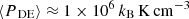 computed via Eq. (9) (the threshold value is shown as a contour overlaid on the galaxy map in the Appendix, Fig. E.1; the corresponding pressure values using the alternative Eq. (8) are
 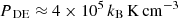 (HCN/CO) and
 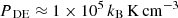 (SFR/HCN)). We note that our cloud-scale ⟨PDE⟩ measurements yield a factor of two to three larger values than the beam-matched 260 pc-scale pressure measurements. For better comparison with previous studies that have no access to ∼100 pc-scale molecular gas measurements, we quote the corresponding threshold pressure values of PDE ≈ 1.5 × 10⁵ to
 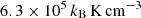 , which consider the CO data convolved to 260 pc-scale (opposed to the weighted average of the 120 pc-scale CO measurements).
4.3.1. HCN/CO versus pressure
We find a strong positive correlation between the (⟨PDE⟩-average) HCN/CO and the ISM pressure, ⟨PDE⟩, in both the high (ρ = 0.64, p = 2.84 × 10⁻³⁴) and low-pressure regime (ρ = 0.79). The correlation is steeper in the high-pressure (m = 0.42 ± 0.03) regime compared to the low-pressure regime (m = 0.18 ± 0.03). However, the realtion could also be well fitted with a single linear function with m = 0.35 ± 0.02. Thus, the average HCN/CO increases in a roughly uniform way from  to
to  suggesting that the ISM pressure is well correlated with the average HCN/CO (ρ = 0.75) over almost three orders of magnitude in pressure.
4.3.2. SFR/HCN versus pressure
In the high-pressure regime we find a moderate negative correlation (ρ = −0.39, p = 0.003,m = −0.89 ± 0.22) between the (⟨PDE⟩-average) SFR/HCN and ISM pressure extending over two order of magnitude in x- and y-axis. In the low-pressure regime the relation is significantly flatter (m = −0.32 ± 0.04) than in the high-pressure regime showing that across the disc, where the ISM pressure is low, SFR/HCN seems to partly decouple from the environmental pressure. However, in both regimes, there is a significant scatter (0.39 dex to 0.54 dex) about the average relation indicating that SFR/HCN is likely affected by other physical conditions than just the pressure or cloud properties (see Appendix D.1), for example, star-formation timescales or gas dynamics, where the latter could play a major role in galaxy centres and bars.
4.4. Morphological environments
In the next step, we analyse the individual morphological environments (centre, bar, bar ends, spiral arms, and interarm, as in Sect. 4.1) in the above-discussed scaling relations. The radial relations (Fig. 7) show that the centre and bar are well separated from the other environments as a function of galactocentric radius, completely dominating the strong negative (HCN/CO) and positive (SFR/HCN) trends with rgal. At larger radii, that is, rgal ≳ 2.5 kpc, we found several overlapping environments (bar, bar ends, spiral arms, and interam) as a function of radius. The mean trends of the HCN/CO and SFR/HCN versus rgal relation for each environment show an identical behaviour as the global relation shown in Sect. 4.4 and we do not find a difference between these environments.
In the HCN/CO versus ⟨PDE⟩ relation (top row of Fig. 8), we observe parallel trends among all environments, with the bar ends and the centre being shifted to higher HCN/CO values (following the mean trends presented as coloured lines). Spiral arms and interarm regions show similar HCN/CO versus pressure relations suggesting that in these environments the molecular clouds have a similar mean density.
 |
Fig. 7. Dense gas spectroscopic ratios versus radius in different morphological environments. Similar to Fig. 6 (left panels), but separately for each environment (compare with right map in Fig. 3). The lighter markers denote low-significant (S/N < 3) data. The grey solid line shows the trend of the spectral stacks as in Fig. 6 (red markers). The coloured lines indicate the stacked measurements of the respective environments taken over all CO detected data (i.e. including HCN non-detections) in the respective environment. |
 |
Fig. 8. Dense gas spectroscopic ratios versus pressure in different morphological environments. Similar to Fig. 7, but as a function of the dynamical equilibrium pressure. |
In the SFR/HCN versus ⟨PDE⟩ relations (bottom row of Fig. 8) the strong trend in the high-pressure regime is again dominated by the centre where SFR/HCN drops by one order of magnitude with increasing ISM pressure. Comparing spiral arms and interarm regions, we find very similar, almost flat trends showing that spiral arms and interarm regions have similar SFR/HCN across 1 dex to 2 dex of ISM pressure and that across the disc SFR/HCN is less dependent on the ISM pressure. In the bar ends we also find a flat trend as a function of pressure but shifted to lower SFR/HCN compared to the disc. The bar, despite having an HCN/CO similar to the disc, shows a much lower SFR/HCN across the whole range of the ISM pressure, which is more consistent with the values found in the centre. This shows that the bar region is a peculiar environment regarding its star-formation properties (see Sect. 5.3 for further discussion).
4.5. HCN/CO as a density tracer
Extragalactic studies of nearby galaxies at kiloparsec-scales (e.g. Gallagher et al. 2018b; Jiménez-Donaire et al. 2019), report a positive correlation of the HCN/CO line ratio with the kiloparsec-scale molecular gas surface density (Σmol) as traced by the CO line intensity over more than two orders of magnitude. These observational results are supported by theoretical works that show that HCN/CO is expected to positively correlate with the dense gas fraction and the mean gas density (Leroy et al. 2017). The physical interpretation put forward for explaining the strong relation between HCN/CO and Σmol is that HCN/CO is expected to trace the density distribution of molecular clouds within the beam. This interpretation is strongly supported by recent works (Gallagher et al. 2018a; Neumann et al. 2023a) that compared the kiloparsec-scale HCN/CO with the cloud-scale Σmol finding a strong positive correlation. Recently, Tafalla et al. (2023) measured the HCN/CO versus H2 column density relation in three solar neighbourhood clouds, finding a similar, strong positive correlation, at least qualitatively in agreement with the extragalactic results.
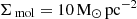
With the new 260 pc-scale HCN observations of NGC 4321, we can now take the next step and study the relation between HCN/CO and Σmol at sub-kiloparsec scales, making these results more comparable to galactic works. In Fig. 9, we present the relation between the HCN(1–0)-to-CO(1–0) line ratio and Σmol, measured at 260 pc resolution. Here, Σmol is inferred from the CO(2–1) line intensity using the lower-resolution R21 map and the surface density-metallicity based αCO prescription as described in Sect. 3.2. We note, that here we use the HCN/CO(1–0), inferred from the CO(2–1) using the estimated R21, instead of the HCN/CO(2–1) line ratio in order to better compare with literature relations. The resulting dense gas fraction, fdense, shown as a secondary y-axis, is computed using a MW-based, constant  and a constant
  . Hence fdense is assumed to be proportional to HCN/CO(1–0) (Appendix A.1).
 |
Fig. 9. HCN/CO versus Σmol relation. Here, we converted the CO(2–1) intensities into CO(1–0) intensities using the R21 map introduced in Appendix A.1. Markers show 260 pc sightline measurements from NGC 4321, with dark blue markers denoting significant (S/N ≥ 3) data. The fit line was obtained by linear regression using LinMix to the stacked measurements (red hexagons) excluding data below |
Analogous to previous sections and following Sect. 3.8, we stacked and fit the data to obtain the mean relation:
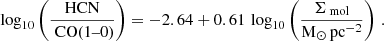
We list the relation parameters along with uncertainties and relations from the literature in Table 5. We note that we exclude data below  (shaded region in Fig. 9) from the fit, because at lower surface densities the trend does not seem to continue in the same manner. This could indicate that at low surface densities, HCN/CO does not increase with Σmol anymore. Santa-Maria et al. (2023) argued that this could be due to HCN being excited in hot, low-surface density regions. However, due to a lack of sensitivity below
  , we could not test this hypothesis with our data. We stress that such a trend can be the result of low completeness thus reflecting the biased-high average HCN/CO if either HCN and CO are clipped (
 ) or if the x-axis is not complete. First and foremost, at
  , we find a strong positive correlation between HCN/CO and Σmol, which agrees well with much of the prior literature. Though, the scatter in the individual 260 pc sightline measurements is twice as large (0.28 dex) as the scatter at kiloparsec-scales (0.14 dex). The larger scatter at smaller scales indicates strong cloud-to-cloud variations in qualitative agreement with galactic studies finding large fdense variations (e.g. Moore et al. 2012; Eden et al. 2012; Csengeri et al. 2016; Urquhart et al. 2021; Tafalla et al. 2023). One explanation for the increased scatter at smaller scales can be cloud evolution effects, leading to changes in the HCN/CO line ratio over the life cycle of molecular clouds, which can only be resolved at smaller scales (e.g. Kruijssen & Longmore 2014). Tafalla et al. (2023) suggest that some of the variations are caused by gas temperature variations between clouds, affecting the HCN excitation. In addition, HCN (and CO) emissivity can be affected by optical depth (Shirley 2015; Leroy et al. 2017; Jiménez-Donaire et al. 2017; Jones et al. 2023; García-Rodríguez et al. 2023) and electron excitation (Goldsmith & Kauffmann 2017), further driving the scatter about the relation. Certainly, in-depth investigations of HCN at higher resolution in nearby galaxies are needed to understand what is driving HCN/CO at fixed surface density.
HCN/CO(1–0) vs. Σmol relations.
Comparing with previous literature findings, the exact relations vary significantly between different studies. The reported slopes span values from 0.41 over 0.61 (this work) to 0.81. Neumann, Jiménez-Donaire et al. in prep. combine measurements from EMPIRE (Jiménez-Donaire et al. 2019) and ALMOND (Neumann et al. 2023b) and match methodologies to obtain an updated, more robust constraint on the HCN/CO versus Σmol relation at kiloparsec-scales, yielding a slope of 0.59 consistent with the slope found for NGC 4321 in this work. Some of the differences between studies can at least partially be attributed to different methodologies. For instance, the adopted αCO prescription significantly affects the measured relation. For NGC 4321, using a constant αCO yields a shallower relation (slope of 0.48) compared to 0.61 with a varying αCO using the prescription described by Eq. (A.2). Moreover, the physical scales observed can significantly affect slopes (Gallagher et al. 2018a found a slope of 0.41 at 2.8 kpc-scale opposed to 0.81 at 650 pc-scale). In addition, using CO(2–1) instead of CO(1–0) will affect the slope if a constant R21 is used to convert CO(2–1) to CO(1–0), making the slope flatter than a native CO(1–0) measurement, since R21 negatively correlates with Σmol (Leroy et al. 2022). For these reasons, comparisons between different studies have to be taken with care. Nevertheless, we want to stress that, independent of methodologies, HCN/CO, at least qualitatively, robustly traces the average molecular gas density from sub-parsec to kiloparsec scales.
Even if tracers and methods are matched, the resolution is expected to affect the observed relation if the emission is not beam-filling. EMPIRE (Jiménez-Donaire et al. 2019) and ALMOND (Neumann et al. 2023b) both studied kiloparsec-scale HCN/CO as a function of Σmol. However, ALMOND used (intensity-weighted) cloud-scale (150 pc) Σmol, while EMPIRE used matched-resolution kiloparsec-scale Σmol. Comparing the HCN/CO versus Σmol from EMPIRE and ALMOND, we find a ∼1 dex shift of the relation towards higher Σmol at smaller scales. These results suggest that the CO filling factor is lower by a factor of ∼10 at ∼1 kpc compared to ∼100 pc. Furthermore, increasing the resolution of the HCN measurements, that is, going to smaller-scale HCN/CO measurements, appears to make the relations steeper (see above) and shifted towards higher HCN/CO, suggesting that HCN is clumpier and/or tracing denser gas than CO.
HCN abundance is expected to vary with metallicity due to the strong decrease of nitrogen-bearing species (e.g. HCN) with decreasing metallicity opposed to oxygen-bearing species (e.g. HCO+) (e.g. Braine et al. 2017, 2023). However, across NGC 4321 the metallicity varies by only ∼0.1 dex (see bottom panel of Fig. A.1). Therefore, abundance and optical depth variations connected to metallicity changes are expected to play only a minor role in affecting the HCN emissivity. In the appendix (Fig. E.2), we show how the HCN-to-HCO+ line ratio varies with metallicity across NGC 4321, finding almost no dependence of HCN/HCO+ on metallicity, supporting the aforementioned statement that HCN is yielding similar results as other dense gas tracers. To further support this statement, we investigated the same scaling relations that are shown in Fig. 6, replacing HCN by HCO+ as a dense gas tracer, yielding the same trends with rgal and ⟨PDE⟩. The average relations agree within 10% with the HCN results except for the central ∼1 kpc, where HCN is about 30% brighter than the average line ratio value of  .
.
We note that the trend expressed by Eq. (10) could be driven by the centre, where we find the strongest systematic variations in HCN/CO. If HCN/CO is interpreted as fdense, we expect the highest centre-to-disc variations in the αCO and αHCN conversion factors in the centre caused, for example, by strong variations in optical depth and excitation temperature, which could additional affect the correlation between fdense and Σmol. We checked that both the centre and the disc show a significant positive correlation between HCN/CO and Σmol with slopes of 0.25 (centre) and 0.35 (disc), which shows that even when the centre is excluded there is a clear dependence of HCN/CO on Σmol. However, the relations in the individual environments are much flatter compared to the overall trend (slope of 0.61) and offset by about 0.4 dex, which indicates that the overall HCN/CO versus Σmol trend might be enhanced by a centre-to-disc dichotomy.
5. Discussion
5.1. Pressure threshold for dense gas and star formation
Over the last decade, resolved kiloparsec-scale observations of nearby galaxies have found a systematic correlation between high-critical density tracer ratios (i.e. HCN/CO and SFR/HCN) and the environmental pressure in the ISM disc (e.g. Gallagher et al. 2018b,a; Jiménez-Donaire et al. 2019; Neumann et al. 2023b). These results are qualitatively supported by observations of the Milky Way’s CMZ, where the star formation efficiency of the (dense) molecular gas is low (Longmore et al. 2013; Kruijssen et al. 2014; Henshaw et al. 2023). These results contrast with solar neighbourhood results that tend to find a constant SFR/HCN (e.g. Heiderman et al. 2010; Lada et al. 2010, 2012; Evans et al. 2014). However, these solar neighbourhood observations probe a much lower ISM pressure environment ( ) than typical extragalactic works. The apparent tension between the galactic and extragalactic works could, however, be solved if there existed a pressure threshold above which cloud properties and hence the observed spectroscopic ratios depend on pressure. Below this threshold, the clouds would be able to decouple from the environment and show universal behaviour in converting the dense gas to stars, a concept also put forward by theoretical works (e.g. Krumholz & Thompson 2007; Ostriker et al. 2010; Krumholz et al. 2012). Gallagher et al. (2018b) suggests that this pressure threshold could be at
  , which is similar to the internal pressure of a typical GMC with
  . We note that our formulation of the ISM pressure includes both the environment (gas and stellar mass) as well as cloud-scale molecular gas mass leading to a factor of 2–3 higher PDE values compared to the purely kiloparsec-scale environmental PDE (Sun et al. 2020). Therefore, the exact value of the pressure threshold is likely to vary with the resolution at which the pressure is measured.
With the new wide-field, deep HCN observations of NGC 4321 presented in this work, we can now for the first time explore the low-pressure environment ( ) at 260 pc scales in a Milky Way-like galaxy and address whether there is a pressure threshold for dense gas and star formation. In Figure 6 (right panels), we determined two pressure regimes in each of the relations based on the change in the behaviour of the mean trends using the methodology described in Sect. 3.8. Focusing on the SFR/HCN versus ⟨PDE⟩ relation, we find a clear negative correlation at high pressures that significantly flattens in the low-pressure regime (especially evident in the mean trends of the individual environments), with the threshold being at
  . Thus, our results might support the pressure threshold hypothesis laid out above (slope changes by 30%), though finding a threshold that is one order of magnitude higher than the value inferred from simple theoretical considerations (
 ). We note, however, that the measured pressure estimates depend strongly on the scales at which they are measured. Sun et al. (2020) show that larger physical scales (∼1 kpc) can lead to lower pressure estimates due to averaging out GMC-scale (∼100 pc) variations of the molecular gas. Therefore, even higher resolution observations (≲100 pc) are needed to obtain robust quantitative pressure estimates comparable with solar neighbourhood measurements.
In the appendix, we also present the relations between the spectroscopic ratios and the 120 pc-scale molecular gas properties (Fig. D.1) representing the self-gravity term on the ISM pressure as well as the relation with stellar mass surface density (Fig. D.2) representing the environment term. We find that a threshold-like behaviour is only seen in the cloud property relation, where SFR/HCN becomes almost constant in the low-Σmol, low-σmol regime. In contrast, SFR/HCN shows a monotonic negative relation with Σ⋆ suggesting that clouds are always connected to the environmental pressure, but in the low-pressure environment the amount of dense gas is converted into stars in a uniform way independent of the cloud-scale properties.
5.2. Normal star formation efficiency in bar ends
Observations (e.g. Kenney & Lord 1991; Harada et al. 2019; Sormani & Barnes 2019; Yu et al. 2022b,a) and simulations (e.g. Sormani et al. 2018) show that gas inflow from the spiral arms and gas outflow from the bar can feed the bar ends with molecular gas. As a consequence, the bar ends are the principal site for cloud-cloud collisions, which are thought to either boost (e.g. Habe & Ohta 1992; Benjamin et al. 2005; López-Corredoira et al. 2007; Furukawa et al. 2009; Ohama et al. 2010; Fukui et al. 2014; Renaud et al. 2015; Fukui et al. 2016, 2018; Torii et al. 2017; Sormani et al. 2020) or lower (e.g. Fujimoto et al. 2020) the formation of stars, depending on the relative speed of the colliding clouds (e.g. Takahira et al. 2014). This raises the question as to whether bar ends boost or suppress star formation. In accordance with the picture that bar ends are fed by gas flows, we observe relatively bright HCN and CO emission, implying an accumulation of (dense) molecular gas in the bar ends. However, we do not find an increased SFEdense, traced by SFR/HCN, compared to the rest of the disc (spiral arms and interarm), suggesting that collisions might enhance density but not necessarily lead to different processes in the dense gas. We discuss the bar environment in the following subsection (Sect. 5.3).
5.3. Star formation suppression in the bar
Galactic bars are the sites of strong shear and gas streaming motions, which can potentially affect the (density) structure of molecular clouds and their ability to form stars (e.g. Athanassoula 1992; Emsellem et al. 2015; Sormani et al. 2018). Díaz-García et al. (2021) find that bar strength can affect quenching, suggesting that bars are loci of suppressed star formation. However, Fraser-McKelvie et al. (2020) also find evidence for increased star formation along bars. Maeda et al. (2023) propose that the star formation efficiency of molecular gas (SFR/CO; SFEmol) in nearby spiral galaxies is systematically suppressed in bars. Here, we go a step further and study the denser molecular gas (traced by HCN) that is more tightly related to SFR and its star formation efficiency, SFEdense. On the one hand, we find very similar HCN/CO, tracing fdense, in the bar as well as throughout the disc. Additionally, we observe the same average trend with ISM pressure as in all other environments suggesting that bars contain clouds with similar mean density than galaxy discs. On the other hand, the agreement with disc trends changes for the dense gas star formation efficiency (SFEdense traced by SFR/HCN), which is much lower than in the disc. The systematically lower SFR/HCN in the bar becomes even more evident in the relation with pressure, where the average trend of the bar is ≈0.5 dex lower compared to the other environments. This suggests that the bar of NGC 4321 is indeed much less efficient in converting dense molecular gas into stars despite the presence of overdense gas.
One explanation for the low SFEdense could be shearing motions inside the bar that are solenoidal in nature, lowering the star formation efficiency (e.g. Federrath et al. 2016) or high-speed cloud-cloud collisions (e.g. Fujimoto et al. 2020). Recent simulations (e.g. Sormani et al. 2018) and observations (Wallace et al. 2022) suggest that gas dynamics in the bar are more dominated by streaming motions from the bar ends towards the galactic centre. These streaming motions can result in deformation and stretching of the molecular clouds in the bar leading to elongated, destructed molecular clouds, which might counteract the gravitational collapse hence quenching star formation.
6. Conclusions
We have presented new deep wide-field HCN(1–0) dense molecular gas observations at scales of 260 pc of the nearby spiral galaxy NGC 4321. By combining recent high-resolution (∼1″ ∼ 100 pc) observations of CO (PHANGS–ALMA; Leroy et al. 2021b) tracing the bulk molecular gas and Hα observations (PHANGS–MUSE; Emsellem et al. 2022) tracing SFR (supported by 21 μm observations from PHANGS–JWST (Lee et al. 2023)), we were able to study for the first time dense gas spectroscopic ratios (HCN/CO, SFR/HCN) in many individual sight lines and environments expanding into the low-pressure regime that is similar to the solar neighbourhood environment. We used morphological masks based on the stellar mass content (Querejeta et al. 2021) to distinguish between different environmental regions that have different structural and dynamical properties that potentially affect the properties of molecular clouds and their ability to form stars. We have studied how HCN/CO, a proxy of the dense gas fraction (fdense), and SFR/HCN, a proxy of the dense gas star formation efficiency (SFEdense), vary between different galactic environments and depend on the ISM pressure. Our key findings are as follows:
-
The HCN/CO increases and SFR/HCN decreases towards the centre of the galaxy, and they are roughly flat across the galactic disc. This suggests that galaxy centres have denser molecular clouds, but they are less efficiently converted into stars than in the disc. These global trends are consistent with previous results from kiloparsec-scale surveys, but our superior resolution allowed us to analyse the role of the environment in more detail. Distinguishing between environmental regions (centre, bar, bar ends, spiral arms, and interarm), we find HCN/CO to be significantly higher in the centre, while SFR/HCN is lower in both the centre and the bar. This shows that the star-formation process is roughly universal across the disc of NGC 4321. In particular, we found no significant difference of HCN/CO and SFR/HCN between the spiral arms and interarm regions, but star formation from the dense gas is significantly less efficient in the bar and centre. The strong trends towards the centre of NGC 4321 suggest either that clouds couple strongly to the surrounding environment or that HCN traces more of the bulk molecular gas that is less efficiently converted into stars, the latter being in agreement with predictions from gravoturbulent cloud models.
-
The mean dense gas spectroscopic trends in the disc (rgal ≳ 2 kpc) of NGC 4321 are very similar among different environments (Fig. 7, Fig. 8). However, we observed a significant scatter of 0.14 dex to 0.54 dex in all relations at fixed radius or fixed pressure. This indicates that, although they are on average similar, cloud properties and their environment vary more significantly at smaller scales and are potentially strongly affected by local cloud-scale (≲100 pc) physics and local excitation conditions (e.g. gas temperature, optical depth).
-
We identified a pressure threshold for dense gas and star formation at
 (Eq. (9); Fig. 6) corresponding to 260 pc-scale
  (Eq. (8)). While the relation between pressure and HCN/CO can also be well described by a single relation covering both regimes, the relation with SFR/HCN significantly flattens in the low-pressure regime. This supports the idea that there is a pressure threshold below which the star-formation process in molecular clouds becomes less dependent on the environment, as seen in galactic measurements of molecular clouds. Thus, our findings hint towards resolving the tension between galactic and extragalactic studies of dense gas and star formation.
 -
The bar of NGC 4321 shows a significantly lower SFR/HCN than the disc and is systematically shifted to lower SFR/HCN in relation to the ISM pressure. This is a strong indication that the star formation in the bar is suppressed by shear or streaming motion that prevents the gravitational collapse and thus star formation.
-
We found a strong positive correlation between HCN/CO and Σmol (Fig. 9) with a slope of 0.61 using a varying αCO to compute Σmol (for comparison, a constant αCO yields a slope of 0.48). Our 260 pc-scale results are in agreement with many previous studies from sub-parsec (galactic) to kiloparsec-scales (extragalactic) and support the use of HCN/CO as a powerful tracer of molecular cloud average density. We emphasise that the exact relation depends on the methodology and that scatter increases at smaller scales. We found a scale-dependence of the relation likely connected to the beam filling factors of CO and HCN, indicating that HCN emission traces denser gas than CO and originates from smaller than 260 pc-scale regions.
These findings present the next step in connecting extragalactic and galactic studies of dense gas and star formation. Overall, our results indicate the presence of a pressure threshold for dense gas and star formation and highlight the potential to link galactic and extragalactic works. However, we are still not able to resolve individual GMCs (≲100 pc) in galaxies beyond the Local Group and explore conditions similar to the solar neighbourhood ( ). Even deeper observations of dense gas tracers are needed to find better constraints on spectroscopic dense gas ratios in the solar neighbour-like low-pressure environment. Moreover, we show that across the disc, SFR tracers yield similar results, but towards the centre, they can differ a lot, hence requiring more in-depth studies of galaxy centres to infer robust prescriptions of dense gas and star formation in these extreme environments. Further, this work only investigated a single galaxy. Ultimately, we need similar dense gas studies in a large sample of galaxies (as done in PHANGS) to study, for example, the effect of bar dynamics on the star formation efficiency or the pressure threshold hypothesis in a statistically meaningful sample of galaxies. Besides, the scale-dependence of the HCN/CO versus Σmol relation requires a more detailed study, particularly to address the CO and HCN filling factors at sub-100 pc scales.
Data availability
The reduced data cubes are available at the CDS via anonymous ftp to cdsarc.cds.unistra.fr (130.79.128.5) or via https://cdsarc.cds.unistra.fr/viz-bin/cat/J/A+A/691/A121 and at https://www.canfar.net/storage/vault/list/phangs/RELEASES/Neumann_et_al_2024
We do not use the archival CO(1–0) observations as a tracer of molecular gas because of their poorer angular resolution (4″, corresponding to ∼300 pc), but we do use them to inform our conversion of CO(2–1) intensity to molecular gas surface density, as described later in Sect. 3.2.
We note that many previous works (e.g. Gao & Solomon 2004) used a slightly smaller value of  tracing gas above nH2 ≈ 3 × 104 cm−3. However, choosing a different (constant) αHCN has no qualitative effect on our results.
https://linmix.readthedocs.io/en/latest/index.html; LinMix is a Bayesian inference tool to linear regression, which can take into account upper limits and infers the posterior distribution of the fit line parameters via MCMC simulation (Kelly 2007).
Acknowledgments
We would like to thank the referee Jonathan Braine for his insightful comments and constructive feedback that helped improve the quality of the paper. This work was carried out as part of the PHANGS Collaboration. LN acknowledges funding from the Deutsche Forschungsgemeinschaft (DFG, German Research Foundation) - 516405419. AKL gratefully acknowledges support by grants 1653300 and 2205628 from the National Science Foundation, by award JWST-GO-02107.009-A, and by a Humboldt Research Award from the Alexander von Humboldt Foundation. The work of AKL is partially supported by the National Science Foundation under Grants No. 1615105, 1615109, and 1653300. AU acknowledges support from the Spanish grants PID2019-108765GB-I00, funded by MCIN/AEI/10.13039/501100011033, and PID2022-138560NB-I00, funded by MCIN/AEI/10.13039/501100011033/FEDER, EU. ER acknowledges the support of the Natural Sciences and Engineering Research Council of Canada (NSERC), funding reference number RGPIN-2022-03499. MB gratefully acknowledges support from the ANID BASAL project FB210003 and from the FONDECYT regular grant 1211000. MC gratefully acknowledges funding from the DFG through an Emmy Noether Research Group (grant number CH2137/1-1). COOL Research DAO is a Decentralized Autonomous Organization supporting research in astrophysics aimed at uncovering our cosmic origins. KG is supported by the Australian Research Council through the Discovery Early Career Researcher Award (DECRA) Fellowship (project number DE220100766) funded by the Australian Government. KG is supported by the Australian Research Council Centre of Excellence for All Sky Astrophysics in 3 Dimensions (ASTRO 3D), through project number CE170100013. JDH gratefully acknowledges financial support from the Royal Society (University Research Fellowship; URF/R1/221620). HAP acknowledges support by the National Science and Technology Council of Taiwan under grant 110-2112-M-032-020-MY3. MQ acknowledges support from the Spanish grant PID2019-106027GA-C44, funded by MCIN/AEI/10.13039/501100011033. TS acknowledges funding from the European Research Council (ERC) under the European Union’s Horizon 2020 research and innovation programme (grant agreement No. 694343). ES acknowledges funding from the European Research Council (ERC) under the European Union’s Horizon 2020 research and innovation programme (grant agreement No. 694343). SKS acknowledges financial support from the German Research Foundation (DFG) via Sino-German research grant SCHI 536/11-1. Y-HT acknowledges funding support from NRAO Student Observing Support Grant SOSPADA-012 and from the National Science Foundation (NSF) under grant No. 2108081. TGW acknowledges funding from the European Research Council (ERC) under the European Union’s Horizon 2020 research and innovation programme (grant agreement No. 694343). This paper makes use of the following ALMA data ADS/JAO.ALMA#2011.0.00004.SV, ADS/JAO.ALMA#2015.1.00956.S, ADS/JAO.ALMA#2017.1.00815.S. ALMA is a partnership of ESO (representing its member states), NSF (USA), and NINS (Japan), together with NRC (Canada), NSC and ASIAA (Taiwan), and KASI (Republic of Korea), in cooperation with the Republic of Chile. The Joint ALMA Observatory is operated by ESO, AUI/NRAO, and NAOJ. The National Radio Astronomy Observatory (NRAO) is a facility of the National Science Foundation operated under cooperative agreement by Associated Universities, Inc.
References
- Anand, G. S., Lee, J. C., Van Dyk, S. D., et al. 2021, MNRAS, 501, 3621 [Google Scholar]
- Athanassoula, E. 1992, MNRAS, 259, 345 [Google Scholar]
- Barnes, A. T., Kauffmann, J., Bigiel, F., et al. 2020, MNRAS, 497, 1972 [NASA ADS] [CrossRef] [Google Scholar]
- Belfiore, F., Leroy, A. K., Sun, J., et al. 2023, A&A, 670, A67 [NASA ADS] [CrossRef] [EDP Sciences] [Google Scholar]
- Bemis, A., & Wilson, C. D. 2019, AJ, 157, 131 [NASA ADS] [CrossRef] [Google Scholar]
- Benincasa, S. M., Wadsley, J., Couchman, H. M. P., & Keller, B. W. 2016, MNRAS, 462, 3053 [NASA ADS] [CrossRef] [Google Scholar]
- Benjamin, R. A., Churchwell, E., Babler, B. L., et al. 2005, ApJ, 630, L149 [NASA ADS] [CrossRef] [Google Scholar]
- Bešlić, I., Barnes, A. T., Bigiel, F., et al. 2021, MNRAS, 506, 963 [CrossRef] [Google Scholar]
- Bešlić, I., Barnes, A. T., Bigiel, F., et al. 2024, A&A, 689, A122 [NASA ADS] [CrossRef] [EDP Sciences] [Google Scholar]
- Bigiel, F., Leroy, A. K., Jiménez-Donaire, M. J., et al. 2016, ApJ, 822, L26 [NASA ADS] [CrossRef] [Google Scholar]
- Blitz, L., & Rosolowsky, E. 2004, ApJ, 612, L29 [NASA ADS] [CrossRef] [Google Scholar]
- Blitz, L., & Rosolowsky, E. 2006, ApJ, 650, 933 [NASA ADS] [CrossRef] [Google Scholar]
- Bolatto, A. D., Wolfire, M., & Leroy, A. K. 2013, ARA&A, 51, 207 [CrossRef] [Google Scholar]
- Braine, J., Shimajiri, Y., André, P., et al. 2017, A&A, 597, A44 [NASA ADS] [CrossRef] [EDP Sciences] [Google Scholar]
- Braine, J., Sun, Y., Shimajiri, Y., et al. 2023, A&A, 676, A27 [NASA ADS] [CrossRef] [EDP Sciences] [Google Scholar]
- Caldú-Primo, A., Schruba, A., Walter, F., et al. 2013, AJ, 146, 150 [CrossRef] [Google Scholar]
- Calzetti, D., Kennicutt, R. C., Engelbracht, C. W., et al. 2007, ApJ, 666, 870 [Google Scholar]
- CASA Team, Bean, B., Bhatnagar, S., et al. 2022, PASP, 134, 114501 [NASA ADS] [CrossRef] [Google Scholar]
- Chen, H., Gao, Y., Braine, J., & Gu, Q. 2015, ApJ, 810, 140 [NASA ADS] [CrossRef] [Google Scholar]
- Chen, H., Braine, J., Gao, Y., Koda, J., & Gu, Q. 2017, ApJ, 836, 101 [NASA ADS] [CrossRef] [Google Scholar]
- Csengeri, T., Weiss, A., Wyrowski, F., et al. 2016, A&A, 585, A104 [NASA ADS] [CrossRef] [EDP Sciences] [Google Scholar]
- den Brok, J. S., Chatzigiannakis, D., Bigiel, F., et al. 2021, MNRAS, 504, 3221 [NASA ADS] [CrossRef] [Google Scholar]
- den Brok, J. S., Bigiel, F., Sliwa, K., et al. 2022, A&A, 662, A89 [CrossRef] [EDP Sciences] [Google Scholar]
- Díaz-García, S., Lisenfeld, U., Pérez, I., et al. 2021, A&A, 654, A135 [NASA ADS] [CrossRef] [EDP Sciences] [Google Scholar]
- Dib, S., Helou, G., Moore, T. J. T., Urquhart, J. S., & Dariush, A. 2012, ApJ, 758, 125 [NASA ADS] [CrossRef] [Google Scholar]
- Eden, D. J., Moore, T. J. T., Plume, R., & Morgan, L. K. 2012, MNRAS, 422, 3178 [NASA ADS] [CrossRef] [Google Scholar]
- Eden, D. J., Moore, T. J. T., Morgan, L. K., Thompson, M. A., & Urquhart, J. S. 2013, MNRAS, 431, 1587 [NASA ADS] [CrossRef] [Google Scholar]
- Eden, D. J., Moore, T. J. T., Urquhart, J. S., et al. 2015, MNRAS, 452, 289 [NASA ADS] [CrossRef] [Google Scholar]
- Eibensteiner, C., Barnes, A. T., Bigiel, F., et al. 2022, A&A, 659, A173 [CrossRef] [EDP Sciences] [Google Scholar]
- Elmegreen, B. G. 1989, ApJ, 338, 178 [NASA ADS] [CrossRef] [Google Scholar]
- Elmegreen, B. G., & Parravano, A. 1994, ApJ, 435, L121 [NASA ADS] [CrossRef] [Google Scholar]
- Emsellem, E., Renaud, F., Bournaud, F., et al. 2015, MNRAS, 446, 2468 [Google Scholar]
- Emsellem, E., Schinnerer, E., Santoro, F., et al. 2022, A&A, 659, A191 [NASA ADS] [CrossRef] [EDP Sciences] [Google Scholar]
- Evans, N. J. I., Heiderman, A., & Vutisalchavakul, N. 2014, ApJ, 782, 114 [CrossRef] [Google Scholar]
- Evans, N. J. I., Kim, K.-T., Wu, J., et al. 2020, ApJ, 894, 103 [NASA ADS] [CrossRef] [Google Scholar]
- Federrath, C., Rathborne, J. M., Longmore, S. N., et al. 2016, ApJ, 832, 143 [NASA ADS] [CrossRef] [Google Scholar]
- Fisher, D. B., Bolatto, A. D., White, H., et al. 2019, ApJ, 870, 46 [NASA ADS] [CrossRef] [Google Scholar]
- Fraser-McKelvie, A., Aragón-Salamanca, A., Merrifield, M., et al. 2020, MNRAS, 495, 4158 [Google Scholar]
- Friedman, J. H. 1991, Ann. Stat., 19, 1 [NASA ADS] [Google Scholar]
- Fujimoto, Y., Maeda, F., Habe, A., & Ohta, K. 2020, MNRAS, 494, 2131 [NASA ADS] [CrossRef] [Google Scholar]
- Fukui, Y., Ohama, A., Hanaoka, N., et al. 2014, ApJ, 780, 36 [Google Scholar]
- Fukui, Y., Torii, K., Ohama, A., et al. 2016, ApJ, 820, 26 [Google Scholar]
- Fukui, Y., Torii, K., Hattori, Y., et al. 2018, ApJ, 859, 166 [Google Scholar]
- Furukawa, N., Dawson, J. R., Ohama, A., et al. 2009, ApJ, 696, L115 [Google Scholar]
- Gallagher, M. J., Leroy, A. K., Bigiel, F., et al. 2018a, ApJ, 868, L38 [CrossRef] [Google Scholar]
- Gallagher, M. J., Leroy, A. K., Bigiel, F., et al. 2018b, ApJ, 858, 90 [NASA ADS] [CrossRef] [Google Scholar]
- Gao, Y., & Solomon, P. M. 2004, ApJ, 606, 271 [NASA ADS] [CrossRef] [Google Scholar]
- García-Burillo, S., Usero, A., Alonso-Herrero, A., et al. 2012, A&A, 539, A8 [Google Scholar]
- García-Rodríguez, A., Usero, A., Leroy, A. K., et al. 2023, A&A, 672, A96 [NASA ADS] [CrossRef] [EDP Sciences] [Google Scholar]
- Gardner, J. P., Mather, J. C., Abbott, R., et al. 2023, PASP, 135, 068001 [NASA ADS] [CrossRef] [Google Scholar]
- Goldsmith, P. F., & Kauffmann, J. 2017, ApJ, 841, 25 [Google Scholar]
- Habe, A., & Ohta, K. 1992, PASJ, 44, 203 [NASA ADS] [Google Scholar]
- Harada, N., Sakamoto, K., Martín, S., et al. 2018, ApJ, 855, 49 [Google Scholar]
- Harada, N., Sakamoto, K., Martín, S., et al. 2019, ApJ, 884, 100 [NASA ADS] [CrossRef] [Google Scholar]
- Hassani, H., Rosolowsky, E., Leroy, A. K., et al. 2023, ApJ, 944, L21 [NASA ADS] [CrossRef] [Google Scholar]
- Heiderman, A., Evans, N. J. I., Allen, L. E., Huard, T., & Heyer, M. 2010, ApJ, 723, 1019 [Google Scholar]
- Henshaw, J. D., Barnes, A. T., Battersby, C., et al. 2023, ASP Conf. Ser., 534, 83 [NASA ADS] [Google Scholar]
- Herrera-Camus, R., Bolatto, A., Wolfire, M., et al. 2017, ApJ, 835, 201 [NASA ADS] [CrossRef] [Google Scholar]
- Jiménez-Donaire, M. J., Bigiel, F., Leroy, A. K., et al. 2017, MNRAS, 466, 49 [CrossRef] [Google Scholar]
- Jiménez-Donaire, M. J., Bigiel, F., Leroy, A. K., et al. 2019, ApJ, 880, 127 [CrossRef] [Google Scholar]
- Jiménez-Donaire, M. J., Usero, A., Bešlić, I., et al. 2023, A&A, 676, L11 [NASA ADS] [CrossRef] [EDP Sciences] [Google Scholar]
- Jones, G. H., Clark, P. C., Glover, S. C. O., & Hacar, A. 2023, MNRAS, 520, 1005 [NASA ADS] [CrossRef] [Google Scholar]
- Kauffmann, J., Goldsmith, P. F., Melnick, G., et al. 2017, A&A, 605, L5 [NASA ADS] [CrossRef] [EDP Sciences] [Google Scholar]
- Kelly, B. C. 2007, ApJ, 665, 1489 [Google Scholar]
- Kenney, J. D. P., & Lord, S. D. 1991, ApJ, 381, 118 [NASA ADS] [CrossRef] [Google Scholar]
- Kennicutt, R. C., & Evans, N. J. 2012, ARA&A, 50, 531 [NASA ADS] [CrossRef] [Google Scholar]
- Kepley, A. A., Leroy, A. K., Frayer, D., et al. 2014, ApJ, 780, L13 [Google Scholar]
- Kepley, A. A., Bittle, L., Leroy, A. K., et al. 2018, ApJ, 862, 120 [NASA ADS] [CrossRef] [Google Scholar]
- Kim, C.-G., & Ostriker, E. C. 2015, ApJ, 815, 67 [NASA ADS] [CrossRef] [Google Scholar]
- Kim, C.-G., Kim, W.-T., & Ostriker, E. C. 2011, ApJ, 743, 25 [NASA ADS] [CrossRef] [Google Scholar]
- Kim, C.-G., Ostriker, E. C., & Kim, W.-T. 2013, ApJ, 776, 1 [NASA ADS] [CrossRef] [Google Scholar]
- Koyama, H., & Ostriker, E. C. 2009, ApJ, 693, 1346 [NASA ADS] [CrossRef] [Google Scholar]
- Kregel, M., van der Kruit, P. C., & de Grijs, R. 2002, MNRAS, 334, 646 [NASA ADS] [CrossRef] [Google Scholar]
- Kroupa, P. 2001, MNRAS, 322, 231 [NASA ADS] [CrossRef] [Google Scholar]
- Kruijssen, J. M. D., & Longmore, S. N. 2014, MNRAS, 439, 3239 [NASA ADS] [CrossRef] [Google Scholar]
- Kruijssen, J. M. D., Longmore, S. N., Elmegreen, B. G., et al. 2014, MNRAS, 440, 3370 [Google Scholar]
- Krumholz, M. R., & McKee, C. F. 2005, ApJ, 630, 250 [Google Scholar]
- Krumholz, M. R., & Thompson, T. A. 2007, ApJ, 669, 289 [NASA ADS] [CrossRef] [Google Scholar]
- Krumholz, M. R., Dekel, A., & McKee, C. F. 2012, ApJ, 745, 69 [Google Scholar]
- Lada, C. J., Lombardi, M., & Alves, J. F. 2010, ApJ, 724, 687 [Google Scholar]
- Lada, C. J., Forbrich, J., Lombardi, M., & Alves, J. F. 2012, ApJ, 745, 190 [NASA ADS] [CrossRef] [Google Scholar]
- Lang, P., Meidt, S. E., Rosolowsky, E., et al. 2020, ApJ, 897, 122 [CrossRef] [Google Scholar]
- Lee, J. C., Whitmore, B. C., Thilker, D. A., et al. 2022, ApJS, 258, 10 [NASA ADS] [CrossRef] [Google Scholar]
- Lee, J. C., Sandstrom, K. M., Leroy, A. K., et al. 2023, ApJ, 944, L21 [NASA ADS] [CrossRef] [Google Scholar]
- Leroy, A. K., Walter, F., Brinks, E., et al. 2008, AJ, 136, 2782 [Google Scholar]
- Leroy, A. K., Walter, F., Bigiel, F., et al. 2009, AJ, 137, 4670 [Google Scholar]
- Leroy, A. K., Usero, A., Schruba, A., et al. 2017, ApJ, 835, 217 [NASA ADS] [CrossRef] [Google Scholar]
- Leroy, A. K., Sandstrom, K. M., Lang, D., et al. 2019, ApJS, 244, 24 [Google Scholar]
- Leroy, A. K., Hughes, A., Liu, D., et al. 2021a, ApJS, 255, 19 [NASA ADS] [CrossRef] [Google Scholar]
- Leroy, A. K., Schinnerer, E., Hughes, A., et al. 2021b, ApJS, 257, 43 [NASA ADS] [CrossRef] [Google Scholar]
- Leroy, A. K., Rosolowsky, E., Usero, A., et al. 2022, ApJ, 927, 149 [NASA ADS] [CrossRef] [Google Scholar]
- Leroy, A. K., Sandstrom, K., Rosolowsky, E., et al. 2023, ApJ, 944, L9 [NASA ADS] [CrossRef] [Google Scholar]
- Licquia, T. C., & Newman, J. A. 2015, ApJ, 806, 96 [NASA ADS] [CrossRef] [Google Scholar]
- Linden, S. T., Murphy, E. J., Dong, D., et al. 2020, ApJS, 248, 25 [NASA ADS] [CrossRef] [Google Scholar]
- Longmore, S. N., Bally, J., Testi, L., et al. 2013, MNRAS, 429, 987 [NASA ADS] [CrossRef] [Google Scholar]
- López-Corredoira, M., Cabrera-Lavers, A., Mahoney, T. J., et al. 2007, AJ, 133, 154 [NASA ADS] [CrossRef] [Google Scholar]
- Maeda, F., Ohta, K., Fujimoto, Y., & Habe, A. 2021, MNRAS, 502, 2238 [NASA ADS] [CrossRef] [Google Scholar]
- Maeda, F., Egusa, F., Ohta, K., Fujimoto, Y., & Habe, A. 2023, ApJ, 943, 7 [NASA ADS] [CrossRef] [Google Scholar]
- Makarov, D., Prugniel, P., Terekhova, N., Courtois, H., & Vauglin, I. 2014, A&A, 570, A13 [NASA ADS] [CrossRef] [EDP Sciences] [Google Scholar]
- Martín, S., Mangum, J. G., Harada, N., et al. 2021, A&A, 656, A46 [NASA ADS] [CrossRef] [EDP Sciences] [Google Scholar]
- Meidt, S. E., Schinnerer, E., van de Ven, G., et al. 2014, ApJ, 788, 144 [Google Scholar]
- Moore, T. J. T., Urquhart, J. S., Morgan, L. K., & Thompson, M. A. 2012, MNRAS, 426, 701 [NASA ADS] [CrossRef] [Google Scholar]
- Murphy, E. J., Bremseth, J., Mason, B. S., et al. 2012, ApJ, 761, 97 [Google Scholar]
- Neumann, L., den Brok, J. S., Bigiel, F., et al. 2023a, A&A, 675, A104 [NASA ADS] [CrossRef] [EDP Sciences] [Google Scholar]
- Neumann, L., Gallagher, M. J., Bigiel, F., et al. 2023b, MNRAS, 521, 3348 [NASA ADS] [CrossRef] [Google Scholar]
- Nguyen-Luong, Q., Anderson, L. D., Motte, F., et al. 2017, ApJ, 844, L25 [NASA ADS] [CrossRef] [Google Scholar]
- O’Donnell, J. E. 1994, ApJ, 422, 158 [Google Scholar]
- Ohama, A., Dawson, J. R., Furukawa, N., et al. 2010, ApJ, 709, 975 [CrossRef] [Google Scholar]
- Onus, A., Krumholz, M. R., & Federrath, C. 2018, MNRAS, 479, 1702 [NASA ADS] [CrossRef] [Google Scholar]
- Ostriker, E. C., & Shetty, R. 2011, ApJ, 731, 41 [Google Scholar]
- Ostriker, E. C., McKee, C. F., & Leroy, A. K. 2010, ApJ, 721, 975 [CrossRef] [Google Scholar]
- Padoan, P., & Nordlund, Å. 2002, ApJ, 576, 870 [NASA ADS] [CrossRef] [Google Scholar]
- Pan, H.-A., & Kuno, N. 2017, ApJ, 839, 133 [NASA ADS] [CrossRef] [Google Scholar]
- Pessa, I., Schinnerer, E., Leroy, A. K., et al. 2022, A&A, 663, A61 [NASA ADS] [CrossRef] [EDP Sciences] [Google Scholar]
- Querejeta, M., Meidt, S. E., Schinnerer, E., et al. 2015, ApJS, 219, 5 [NASA ADS] [CrossRef] [Google Scholar]
- Querejeta, M., Schinnerer, E., Schruba, A., et al. 2019, A&A, 625, A19 [NASA ADS] [CrossRef] [EDP Sciences] [Google Scholar]
- Querejeta, M., Schinnerer, E., Meidt, S., et al. 2021, A&A, 656, A133 [NASA ADS] [CrossRef] [EDP Sciences] [Google Scholar]
- Ragan, S. E., Moore, T. J. T., Eden, D. J., et al. 2016, MNRAS, 462, 3123 [NASA ADS] [CrossRef] [Google Scholar]
- Ragan, S. E., Moore, T. J. T., Eden, D. J., et al. 2018, MNRAS, 479, 2361 [NASA ADS] [CrossRef] [Google Scholar]
- Renaud, F., Bournaud, F., Emsellem, E., et al. 2015, MNRAS, 454, 3299 [NASA ADS] [CrossRef] [Google Scholar]
- Rigby, A. J., Moore, T. J. T., Eden, D. J., et al. 2019, A&A, 632, A58 [NASA ADS] [CrossRef] [EDP Sciences] [Google Scholar]
- Salo, H., Laurikainen, E., Laine, J., et al. 2015, ApJS, 219, 4 [Google Scholar]
- Sánchez-García, M., García-Burillo, S., Pereira-Santaella, M., et al. 2022, A&A, 660, A83 [NASA ADS] [CrossRef] [EDP Sciences] [Google Scholar]
- Santa-Maria, M. G., Goicoechea, J. R., Pety, J., et al. 2023, A&A, 679, A4 [NASA ADS] [CrossRef] [EDP Sciences] [Google Scholar]
- Schinnerer, E., & Leroy, A. K. 2024, ArXiv e-prints [arXiv:2403.19843] [Google Scholar]
- Schinnerer, E., Meidt, S. E., Colombo, D., et al. 2017, ApJ, 836, 62 [NASA ADS] [CrossRef] [Google Scholar]
- Schruba, A., Leroy, A. K., Walter, F., et al. 2011, AJ, 142, 37 [NASA ADS] [CrossRef] [Google Scholar]
- Schruba, A., Kruijssen, J. M. D., & Leroy, A. K. 2019, ApJ, 883, 2 [NASA ADS] [CrossRef] [Google Scholar]
- Sheth, K., Regan, M., Hinz, J. L., et al. 2010, PASP, 122, 1397 [Google Scholar]
- Shetty, R., & Ostriker, E. C. 2012, ApJ, 754, 2 [NASA ADS] [CrossRef] [Google Scholar]
- Shimajiri, Y., André, P., Braine, J., et al. 2017, A&A, 604, A74 [NASA ADS] [CrossRef] [EDP Sciences] [Google Scholar]
- Shirley, Y. L. 2015, PASP, 127, 299 [Google Scholar]
- Sormani, M. C., & Barnes, A. T. 2019, MNRAS, 484, 1213 [NASA ADS] [CrossRef] [Google Scholar]
- Sormani, M. C., Treß, R. G., Ridley, M., et al. 2018, MNRAS, 475, 2383 [NASA ADS] [CrossRef] [Google Scholar]
- Sormani, M. C., Tress, R. G., Glover, S. C. O., et al. 2020, MNRAS, 497, 5024 [Google Scholar]
- Spitzer, L., Jr 1942, ApJ, 95, 329 [NASA ADS] [CrossRef] [Google Scholar]
- Stuber, S. K., Pety, J., Schinnerer, E., et al. 2023, A&A, 680, L20 [NASA ADS] [CrossRef] [EDP Sciences] [Google Scholar]
- Sun, J., Leroy, A. K., Schruba, A., et al. 2018, ApJ, 860, 172 [NASA ADS] [CrossRef] [Google Scholar]
- Sun, J., Leroy, A. K., Ostriker, E. C., et al. 2020, ApJ, 892, 148 [NASA ADS] [CrossRef] [Google Scholar]
- Sun, J., Leroy, A. K., Rosolowsky, E., et al. 2022, AJ, 164, 43 [NASA ADS] [CrossRef] [Google Scholar]
- Tafalla, M., Usero, A., & Hacar, A. 2023, A&A, 679, A112 [NASA ADS] [CrossRef] [EDP Sciences] [Google Scholar]
- Takahira, K., Tasker, E. J., & Habe, A. 2014, ApJ, 792, 63 [Google Scholar]
- Teng, Y.-H., Sandstrom, K. M., Sun, J., et al. 2023, ApJ, 950, 119 [NASA ADS] [CrossRef] [Google Scholar]
- Torii, K., Hattori, Y., Hasegawa, K., et al. 2017, ApJ, 835, 142 [NASA ADS] [CrossRef] [Google Scholar]
- Tress, R. G., Smith, R. J., Sormani, M. C., et al. 2020, MNRAS, 492, 2973 [Google Scholar]
- Urquhart, J. S., Figura, C., Cross, J. R., et al. 2021, MNRAS, 500, 3050 [Google Scholar]
- Usero, A., Leroy, A. K., Walter, F., et al. 2015, AJ, 150, 115 [Google Scholar]
- van der Kruit, P. C. 1988, A&A, 192, 117 [NASA ADS] [Google Scholar]
- Véron-Cetty, M. P., & Véron, P. 2010, A&A, 518, A10 [Google Scholar]
- Viaene, S., Forbrich, J., & Fritz, J. 2018, MNRAS, 475, 5550 [NASA ADS] [CrossRef] [Google Scholar]
- Wallace, J., Battersby, C., Mills, E. A. C., et al. 2022, ApJ, 939, 58 [NASA ADS] [CrossRef] [Google Scholar]
- Walter, F., Brinks, E., de Blok, W. J. G., et al. 2008, AJ, 136, 2563 [Google Scholar]
- Watanabe, Y., Sorai, K., Kuno, N., & Habe, A. 2011, MNRAS, 411, 1409 [NASA ADS] [CrossRef] [Google Scholar]
- Williams, T. G., Kreckel, K., Belfiore, F., et al. 2022, MNRAS, 509, 1303 [Google Scholar]
- Wong, T., & Blitz, L. 2002, ApJ, 569, 157 [CrossRef] [Google Scholar]
- Wright, G. S., Rieke, G. H., Glasse, A., et al. 2023, PASP, 135, 048003 [NASA ADS] [CrossRef] [Google Scholar]
- Yu, S.-Y., Kalinova, V., Colombo, D., et al. 2022a, A&A, 666, A175 [NASA ADS] [CrossRef] [EDP Sciences] [Google Scholar]
- Yu, S.-Y., Xu, D., Ho, L. C., Wang, J., & Kao, W.-B. 2022b, A&A, 661, A98 [NASA ADS] [CrossRef] [EDP Sciences] [Google Scholar]
Appendix A: Ancillary data
A.1. CO-to-H2 conversion factor – αCO
In this work, we employ two different conversion factors to convert the CO(2–1) line intensity into a molecular gas surface density as described in Sect. 3.2.
A.1.1. Constant conversion factor
As a first step, we study variations of the HCN-to-CO line ratio, which is a proxy for the dense gas fraction, adopting constant mass-to-light ratios (Sect. 3.3). We adopt a Milky-Way average CO-to-H2 conversion factor of  that is uncertain by a factor of two (Bolatto et al. 2013). To convert the CO(2–1) into a CO(1–0) line intensity, we use a CO(2–1)-to-CO(1–0) line ratio of R21 = 0.65 ± 0.17 (den Brok et al. 2021; Leroy et al. 2022).
A.1.2. Spatially varying conversion factor
As a second step, we adopt varying conversion factors to obtain the most accurate estimation of the molecular gas surface density given the current knowledge about spatial variations of αCO and R21 in nearby galaxies at ∼100 pc scales. This prescription enters the estimation of the dynamical equilibrium pressure (Sect. 3.6). We convert the CO(2–1) moment-zero (WCO(2–1)) into a molecular gas surface density (Σmol) in a two-step process: First, we convert the CO(2–1) into a CO(1–0) line intensity by applying a spatially varying CO(2–1)-to-CO(1–0) line ratio (R21) map. This makes use of archival CO(1–0) observations of NGC 4321 with ALMA at 4″resolution. Hence we can compute R21 at 4″ ∼ 300 pc scale and infer CO(1–0) from the measured CO(2–1) at 1.67″ ∼ 120 pc resolution:
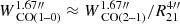
Certainly, we expect small-scale variations of R21 at < 300 pc scales, but using a 300 pc-smoothed R21 still provides more accurate estimates of CO(1–0) and hence Σmol than adopting a constant R21. Here, we measure a median R21 = 0.54 and a scatter of 0.16 dex. We show a map of R21 in Fig. A.1.
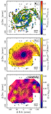 |
Fig. A.1. Conversion factor maps. Top: CO(2–1)-to-CO(1–0) line ratio (R21) map computed from CO(2–1) observations (PHANGS–ALMA) and CO(1–0) observations (ALMA science verification program) at a common 4″resolution. Middle: CO-to-H2 conversion factor (αCO) following the prescription from Bolatto et al. (2013) (Equ. A.2) using metallicities (bottom panel) from PHANGS–MUSE optical recombination lines observations (Williams et al. 2022). |
Next, we converted the inferred CO(1–0) moment-zero map (WCO(1–0)) into Σmol by applying the prescription described by Equation 31 from Bolatto et al. (2013):
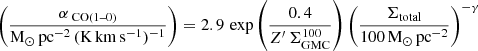
following the iterative approach presented in Sun et al. (2022). Z′ is the local metallicity in units of Solar metallicities, and γ is 0.5 if 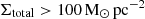 and 0 otherwise. The local metallicity is estimated from optical line measurements taken by MUSE applying a Gaussian Process Regression (GPR) to model the 2D metallicity distribution (Williams et al. 2022). Here,
  is fixed at unity, that is, we adopted a fiducial GMC surface density of
  , and the total surface density (Σtotal) includes molecular gas (CO), atomic gas (H I, Sect. A.2), and stellar mass (3.6 μm, Sect. A.3). Since αCO is implicitly needed to compute Σtotal, Equation A.2 must be solved iteratively. We show a map of the adopted αCO map in Fig. A.1. The median αCO value is
  and thus by a factor of 1.3 lower than the MW based αCO listed above. For this galaxy, αCO systematically decreases by a factor of ∼3 from the disc over the spiral arms towards the centre of NGC 4321, with a scatter of 0.10 dex. Overall, the inferred total H2 mass of the varying αCO across the FOV used in this work is
  , which is lower by a factor of 0.57 than the value obtained via a constant MW-based αCO, yielding
  .
.
We note that Teng et al. (2023) inferred cloud-scale αCO values for the central 2 kpc of NGC 4321 using a multi-line modelling approach based on cloud-scale multi-line, multi-transition CO isotopologues. Despite the existing robust αCO measurement, we employ the surface density-metallicity-based calibration from Bolatto et al. (2013) to obtain continuous αCO values across the full disc of NGC 4321 and note that the measurements from Teng et al. (2023) are on average 0.20 dex smaller than the values used here, but consistent at the 1-sigma level within 0.21 dex.
A.2. Atomic gas – H I 21-cm
We utilise H I 21-cm line observations to measure the atomic gas surface density. The H I data are from VLA observations associated with HERACLES (Leroy et al. 2009) mapping several nearby galaxies in H I at ∼20″ resolution. We converted the integrated intensity of H I (W21cm) into atomic gas surface density via (Walter et al. 2008)
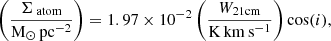
where cos(i) is accounting for the inclination of the galaxy (i = 38.5°).
A.3. Stellar mass – 3.6 μm
We use the stellar mass surface density map from Querejeta et al. (2015), who use 3.6 μm observations from the Spitzer Survey of Stellar Structure in Galaxies (S4G; Sheth et al. 2010). The 3.6 μm maps are corrected for dust attenuation using an “Independent Component Analysis” (ICA) method that separates stars and dust on a pixel-to-pixel basis (for more details, see Querejeta et al. 2015) We converted the attenuation-corrected 3.6 μm map into stellar mass surface density, Σ⋆, via
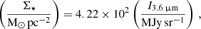
which assumes a constant mass-to-light ratio of 0.6 M⊙/L⊙ (Meidt et al. 2014).
In App. A.4, we use the stellar mass volume density (ρ⋆) to compute the dynamical equilibrium pressure of the ISM in the galaxy disc. We estimated ρ⋆ from the stellar mass surface density, adopting the recipes used in Blitz & Rosolowsky (2006), Leroy et al. (2008), Ostriker et al. (2010), Sun et al. (2020):
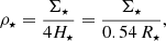
where H⋆ and R⋆ are the scale height and radial scale length of the stellar disc. Above equation assumes an isothermal density profile along the vertical direction (van der Kruit 1988) and a fixed stellar disc flattening ratio of R⋆/H⋆ = 7.3 (Kregel et al. 2002). We adopt R⋆ = 61.1″ ∼ 4.5 kpc from the S4G photometric decomposition analysis (Salo et al. 2015).
A.4. Dynamical equilibrium pressure
We compute the dynamical equilibrium pressure, or ISM pressure (PDE) following the prescription by Sun et al. (2020). PDE describes the pressure regulated by the mass content in the ISM disc and thus provides an important gauge of the local environment of molecular clouds. The distribution of stars and gas in a galaxy disc can approximately be described as isothermal fluids in a plane-parallel geometry. In this prescription, the dynamical equilibrium pressure is composed of a pressure term created by the ISM due to the self-gravity of the ISM disc and a term due to the gravity of the stars (see e.g. Spitzer 1942) such that

where we assumed a smooth, single-fluid gas disc, and that all gas shares a similar velocity dispersion, so that Σgas = Σmol + Σatom is the total gas surface density, ρ⋆ is the stellar mass volume density near disc midplane and σgas,z is the velocity dispersion of the gas perpendicular to the disc.
Sun et al. (2020) proposed a new formalism that takes into account the self-gravity of the molecular gas at high resolution (i.e. 100 pc scale). In this work, we adopted their formalism, which is described in the following. To combine the cloud-scale Σmol, 120 pc data with the large-scale Σatom and ρ⋆, we split PDE into two parts: the pressure of the molecular gas at cloud-scale, Pcloud, and the pressure of the smooth extended atomic gas due to the gravity of all gas (atomic and molecular) and the stars, Patom. The cloud-scale Pcloud consists of three terms accounting for the self-gravity of the molecular gas, the gravity of larger molecular structures, and the gravity of stars:
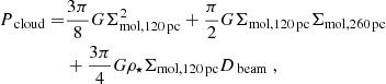
where ρ⋆ is computed as described in App. A.3. In Equ. (A.7), Σmol, 120 pc is given at the cloud-scale resolution (here 120 pc) while Σmol, 260 pc and ρ⋆ describe the distributions of the molecular gas and the stellar mass density at 260 pc scale. In typical units, Equ. (A.7) reads
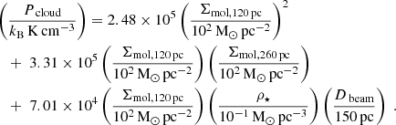
The large-scale Patom includes the self-gravity of the atomic gas and the gravitational interaction of the atomic gas with the (large-scale) molecular gas and the stars:

where σatom is the velocity dispersion of the atomic gas, which is fixed at  . In Equ. (A.9), all quantities are convolved to the large-scale resolution. Converting to typical units, we obtained
Finally, we computed the intensity-weighted average, ⟨Pcloud, 120 pc⟩260 pc, at the large-scale to combine the molecular gas weight with the large-scale Patom pixel by pixel:

Appendix B: Spectral stacking
We compute spectral stacks using the python package PyStacker6 presented in Neumann et al. (2023a). PyStacker uses a high-significance prior (here CO(2–1)) to determine the velocity field of the line emission. It then uses this velocity information to shift the spectra of various line to correct for the Doppler shift, assuming all lines share the same velocity field. Afterwards, we average the shuffled spectra over larger regions usually resulting in higher-significance detections. Here, we stack the emission of CO(2–1) (from PHANGS–ALMA) and HCN(1–0) (this work) via morphological environment (Fig. 4), galactocentric radius, rgal (Fig. B.1), dynamical equilibrium pressure, ⟨PDE⟩ (Fig. B.2), molecular gas surface density (Fig. B.3), Σmol, stellar mass surface density, Σ⋆, and molecular cloud properties, ⟨Σmol⟩, ⟨σmol⟩, ⟨αvir⟩. We use these averaged spectra to compute integrated intensities, where the velocity-integration window is inferred based on the average CO(2–1) spectrum using the same masking method as described in Sect. 3.1. We note that the spectral stacks agree within ±10% with binned integrated intensities computed within the same stacking bins if CO(2–1) is used as a prior to define the velocity-integration mask.
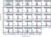 |
Fig. B.1. Similar to to Fig. 4, but using the galactocentric radius, rgal, as the stacking quantity with 0.5 kpc (twice the beam size) bin widths. The panels with hatched background denote radial bins that are not completely covered by the field-of-view of the observations and thus not considered for the radial fit in Fig. 6. |
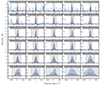 |
Fig. B.2. Similar to to Fig. 4, but using the dynamical equilibrium pressure, ⟨PDE⟩, as the stacking quantity with 0.1 dex bin widths. Note that the bins from ⟨PDE⟩ = 107.0 to |
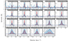 |
Fig. B.3. Similar to to Fig. 4, but using the molecular gas surface density, Σmol, as the stacking quantity with 20 bins from |
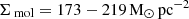

Appendix C: Star formation rate tracers
C.1. Star formation rate – 21 μm
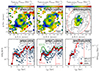 |
Fig. C.1. Comparison of SFR tracer in dense gas scaling relations in the inner 4 kpc. Top: SFR/HCN, tracing dense gas star formation efficiency, using three different SFR tracer from left to right, Hα from MUSE, 21 μm from JWST and 33 GHz from VLA. Contours show HCN intensities as in Fig. 3. The dotted ellipse denotes rgal = 2.75 kpc. Bottom: SFR/HCN, matching the respective above panels, against galactocentric radius, rgal. Blue points indicate detected (S/N ≥ 3) and light blue points denote non-significant (S/N < 3) data. The red hexagon markers show the spectral stacks taken over all data within the bin. In the middle panel, we show the data obtained from the linear 21 μm-to-SFR conversion (Equ. (C.1)) and additionally indicate the mean trend inferred from a power law conversion, that is, SFR ∝ L(F2100W)1.3 (Leroy et al. 2023). |
We use 21 μm (F2100W) emission from recent JWST–MIRI (Gardner et al. 2023; Wright et al. 2023) observations as a another probe of SFR, in addition to Hα from PHANGS–MUSE (Sect. 3.4) and 33 GHz from VLA (Sect. C.2). These data are part of the “PHANGS–JWST Treasury Program” (Lee et al. 2023) and have been reduced via the PHANGS–JWST data reduction pipeline (Williams et al. in prep.). NGC 4321 was observed by JWST in June 2023 and we use version 0.9 of the PHANGS–JWST data reduction.
Physically, the strong radiation field from young, massive stars heat up the surrounding dust, which re-emits at infrared wavelength probed by F2100W. 21 μm point sources correlate well with  regions (Hassani et al. 2023) and the F2100W intensity correlates well, though non-linearly, with extinction-corrected Hα intensity (Leroy et al. 2023; Belfiore et al. 2023). However, the F2100W also captures stochastically heated emission from small dust grains that can trace the ISM. It may thus be both more robust to extinction than Hα and more subject to contamination by diffuse ISM emission.
To infer ΣSFR from F2100, we used the empirical relation from Leroy et al. (2023) (their equation 5), which re-scales the 21 μm flux into a 24 μm flux using R21 μm/24 μm = 0.80 and then converts to SFR via a linear conversion (e.g. following Kennicutt & Evans 2012) such that the SFR surface density is given by

Thus, we adopted a linear relation between F2100W dust emission and the SFR. We also contrast this prescription with a power-law relation based on Leroy et al. (2023), which leads to up to a factor of three higher values in the central ∼2 kpc of NGC 4321.
C.2. Star formation rate – 33 GHz
We note that above SFR tracers might lead to significantly discrepant results in galaxy centres, where optical recombination lines can become too extinct to recover robust Balmer decrement corrections and 21 μm emission might be systematically contaminated by stochastically heated dust grain. Therefore, we use free-free 33 GHz emission from as an additional SFR tracer in the centre of NGC 4321. The data are coming from Very Large Array (VLA) observations of a large sample of galaxies, including NGC 4321, at 3 GHz to 33 GHz at ∼2″ resolution (Linden et al. 2020).
At high radio frequencies the ionising flux of young massive stars is directly proportional to the thermal spectral luminosity. This allowed us to trace the SFR via the thermal part of the 33 GHz flux measured by the VLA following the prescription in Murphy et al. (2012) (their equation 6):
where the thermal fraction (fthermal) values are taken from Linden et al. (2020) (their table 4; ∼200 pc apertures), and we adopted an electron temperature of Te = 104 K and ν = 33 GHz.
C.3. Star formation rate tracer comparison
Throughout this work, we have used Balmer decrement-corrected Hα emission as a tracer of SFR (Sect. 3.4). Despite being a robust tracer of SFR overall, when corrected for dust attenuation, in the centres of galaxies, Hα might miss some of the SFR-related Hα emission due to extremely high attenuation by denser dust thus biasing the SFR estimate high. Also, in extreme environments, like the centre, Hα emission might be associated with other processes than young stars and thus bias the SFR high. Therefore, we tested how robust our findings are against the choice of the SFR tracer, which is laid out in the following.
We use JWST F2100W emission to trace SFR via the hot dust emission that is less affected by attenuation effects in the centre of the galaxy as long as these galaxy centres contain sufficient amounts of dust (Sect. C.1). Using the F2100W-inferred SFR (instead of Hα) leads to similar SFR/HCN values across the disc and in the low-pressure regime for both prescriptions (linear and power-law conversion) adopted here (see Fig. C.1. However, the two calibrations differ by up to a factor of three in the central kiloparsec of the galaxy. The change is so severe that using the power-law calibration yields similar SFRF2100W/HCN values in the centre (median 10−1.05) as in bar ends (median 10−0.96), spiral arms (median 10−1.06) and interarm (median 10−1.19), and statistically the same SFRF2100W/HCN distribution in the centre compared to the aforementioned environments.
In addition, we compared the two SFR tracers (Hα and F2100W) with the 33 GHz-inferred values, as 33 GHz emission is usually considered as the most robust tracer of the SFR in the centres of galaxies (Sect. C.2). We find that Hα (decrement-corrected) and 33 GHz yield very consistent results across the whole central 1 kpc probed by 33 GHz emission, agreeing within 20%. F2100W (linear conversion) leads to a factor of two higher values in the central 260 pc, but otherwise consistent values. Therefore, we conclude that for NGC 4321 Balmer decrement-corrected Hα emission is an excellent tracer of the SFR, even in the centre of the galaxy, where increased dust attenuation could have depreciated Hα as a robust SFR tracer. Moreover, these results suggest that F2100W is proportional to the SFR across the full disc of NGC 4321.
Appendix D: Scaling relations
D.1. Molecular cloud relations
In Fig. D.1, we present the relations between HCN/CO and SFR/HCN respectively with the properties of molecular gas at GMC scales (i.e. here at 120 pc). The cloud-scale molecular gas properties are computed following the prescriptions of Sun et al. (2018) and Neumann et al. (2023b), but adopting the varying αCO and R21 conversions introduced in Sect. A.1.2. We computed the molecular gas surface density from the CO(2–1) integrated intensity (WCO(2–1)):
The molecular gas velocity dispersion was obtained from the CO(2–1) equivalent line width and corrected for the velocity channel-to-channel correlation:
where σmeasured assumes a Gaussian line profile and σresponse takes into account the instrument channel width and channel-to-channel correlation. To estimate the virial parameter (αvir), we assumed spherically symmetric clouds with a given density profile ρ ∝ r−1 so that αvir could be computed from the CO(2–1) data using Σmol and σmol:
where G is the gravitational constant. These molecular gas properties are computed at Dbeam = 120 pc scale and converted to the HCN resolution (i.e. 260 pc) via a Σmol-weighted average, similar to PDE as described in Sect. 3.6, hence the notation ⟨X120 pc⟩260 pc, where X is the quantity to by averaged.
Similar to the relations with radius (Sect. 4.2) and pressure (Sect. 4.3), we apply the MARS linear regression tool (Sect. 3.8) to the cloud property relations shown in Fig. D.1. We find that HCN/CO correlated positively and with Σmol, σmol and αvir and is well-described by a single power law over the whole data range that is probed. Similarly, we observe a negative correlation between SFR/HCN and Σmol, σmol, αvir. However, for SFR/HCN versus Σmol and σmol we find a change in the relation (as determined via MARS) at  and σmol = 8.3 km s−1, such that SFR/HCN is roughly constant at low Σmol (σmol) and strongly decreasing with increasing Σmol (σmol) at high Σmol (σmol).
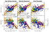 |
Fig. D.1. HCN spectroscopic ratios against molecular cloud properties. Top: HCN/CO and (bottom) SFR/HCN measured at 260 pc scale versus cloud-scale molecular gas properties inferred from 120 pc scale CO(2–1) observations. Panels from left to right show molecular cloud surface density (Σmol), velocity dispersion (σmol) and virial parameter (αvir) on the x-axis, obtained from PHANGS–ALMA as described in Sect. D.1. Similarly to Fig. 7 and 8, markers indicate the respective environments and line fits as well as linear regression regimes are determined via MARS. The obtained thresholds are |

HCN/CO(2 − 1) and SFR/HCN correlations with Σ⋆, ⟨Σmol⟩, ⟨σmol⟩, ⟨αvir⟩.
D.2. Stellar mass relations
Figure D.2 shows the HCN/CO and SFR/HCN scaling relation with the stellar mass surface density, Σ⋆. We compute Σ⋆ from the Spitzer 3.6 μm image as described in Sect. A.3. Following the same methodology as in Sect. 4.2, 4.3, D.1, we determine the power law behaviour of the mean trend finding strong correlations between HCN/CO (positive correlation) and SFR/HCN (negative correlation) with Σ⋆. For HCN/CO versus Σ⋆, we observe a tighter relation (0.19 dex scatter) that is consistent over all environments and the whole probed data range, spanning two orders of magnitude in stellar mass surface density ( to
to  ). The found relation shows that Σ⋆ is a good predictor of HCN/CO over the whole disc of a nearby galaxy at sub-kiloparsec scales, though most of the dynamic range of Σ⋆ is covered by only two regions, the centre and the bar. The relation between SFR/HCN and Σ⋆ shows a much higher scatter (0.46 dex), with the bar region being offset to the main relation by 0.2 dex, stressing the strongly suppressed star formation efficiency in the bar (Sect. 5.3). Combined with the results presented in Sect. D.1, the found relations suggest that the threshold behaviour in the SFR/HCN versus PDE relation (Sect. 4.3) is caused by molecular gas cloud-scale physics rather than larger scale environment.
 |
Fig. D.2. HCN spectroscopic ratio versus stellar mass surface density similar to Fig. 7 and 8, but using Σ⋆ on the x-axis. Stellar mass is traced via the dust-attenuation corrected 3.6 μm emission. The line fit parameters are listed in Tab. D.1. |
Appendix E: Additional figures
Fig. A.1 shows the CO(2–1)-to-CO(1–0) line ratio (R21) computed from the 4″ ∼ 300 pc resolution CO(1–0) data from Pan & Kuno (2017) and homogenised CO(2–1) observations form PHANGS–ALMA (Leroy et al. 2021b). We use the measured 300 pc-scale R21 map to infer the cloud-scale (120 pc) CO(1–0) line intensities from the observed CO(2–1) line intensities, which enter the estimation of the dynamical equilibrium pressure (Sect. 3.6). In Sect. 4.5, we use the R21 map to convert the 260 pc-scale WCO(2–1) into WCO(1–0) to compare the HCN-to-CO(1–0) versus Σmol scaling relation with literature findings.
In Fig. E.1, we show a map of the morphological environments overlaid with HCN contours similar to Fig. 3, right panel. In addition, we indicate two loci of ISM pressure, PDE, matching the pressure thresholds inferred for the HCN/CO and SFR/HCN versus PDE scaling relations (Sect. 4.3).
 |
Fig. E.1. Pressure threshold contours. The map shows the same morphological environment masks as in Fig. 3. Overlaid are HCN contours in grey and ⟨PDE⟩ contours at |


Fig. E.2 presents HCN/CO and HCN/HCO+ line ratio trends with metallicity. Detected sigh line measurements of HCN/CO show no correlation with metallcity (ρPearson = 0.12). The stacked average HCN/CO increases with metallicity, suggesting that the HCN abundance is more strongly depending on metallicity than CO, which is expected if nitrogen decreases more sharply with metallicity than oxygen (Braine et al. 2017, 2023). In this scenario we would expect a systematic increase of the HCN/HCO+ line ratio with metallicity. However, we find only a weak correlation between HCN/HCO+ and metallicity (ρ = 0.35), indicating that metallicity effect play only a minor role across NGC 4321, potentially due to the small dynamic range in metallicity, spanning less than 0.1 dex (8.54 to 8.62).
 |
Fig. E.2. Line ratio trends with metallicity. Top: HCN/CO(2–1) against metallicity Bottom: HCN/HCO+ against metallicity. Dark markers indicate significant data (S/N ≥ 3) and light markers show non-detections (S/N < 3). The red hexagon markers show the average trends over all data obtained via spectral stacking. We note that the HCO+ data will be separately published and studied in more detail along with other dense gas tracers in Neumann et al. in prep. Here, we only show the HCN/HCO+ variation with metallicity to highlight the flat trends hence supporting HCN as a tracer of density across the full molecular gas disc of NGC 4321. |
In Fig. E.3, we display maps of various data products surface density maps of the atomic gas, (dense) molecular gas and stellar mas, ISM pressure and SFR inferred from Hα and 21 μm, respectively. In addition, we show the star formation efficiency of the molecular gas, SFR/CO.
 |
Fig. E.3. Data product maps compilation. All maps are convolved to a common resolution of 260 pc, given by the native resolution of the HCN data, and sampled to a common, hexagonal pixel grid at beam size spacing. |
All Tables
All Figures
|
Fig. 1. JWST three-colour image of NGC 4321 overlaid with HCN contours. The background image is a three-colour composite using the MIRI and NIRCAM instruments observations (red = F770W + F1000W + F1130W + F2100W, green = F360M + F770W, and blue = F300M + F335M) taken from the PHANGS–JWST treasury survey (Lee et al. 2023). Overlaid HCN(1–0) contours (new data presented in this work), tracing the dense molecular gas are drawn at S/N levels of (2, 3, 5, 10, 20, 30, 50, 100). The sites of star formation (reddish hues) appear spatially well correlated with the dense gas traced by HCN. This image is rotated by 21° with respect to the right ascension-declination plane as indicated by the north (N)-east (E) coordinate axes in the bottom left. The bottom right image shows a rgb image (red = F814W, green = F555W, blue = F438W + F336W + F275W) from PHANGS–HST (Lee et al. 2022). |
| In the text | |
|
Fig. 2. NGC 4321 data used in this study, each at the native resolution of the respective observations indicated in the bottom left of each panel. Top left: HCN(1–0) moment-zero map presented in this work. Top right: CO(2–1) moment-zero map from PHANGS–ALMA (Leroy et al. 2021b). Bottom left: Extinction-corrected Hα flux density from PHANGS–MUSE (Emsellem et al. 2022). Bottom right: 21 μm flux density from MIRI-F2100W (PHANGS–JWST; Lee et al. 2023). In each panel, white-to-black-gradient contours show HCN moment-zero signal-to-noise ratio levels of (2, 3, 5, 10, 20, 30, 50, 100) as in Fig. 1. The yellow-coloured outline shows the FOV of the respective observations. |
| In the text | |
|
Fig. 3. NGC 4321 maps sampled at beam size. Left: HCN/CO line ratio map, as a proxy of the dense gas fraction (fdense). The CO(2–1) data are taken from the PHANGS-ALMA survey (Leroy et al. 2021b). Middle: SFR surface density-to-HCN line intensity ratio, as a proxy of the dense gas star formation efficiency (SFEdense). The SFR surface densities are obtained from the Balmer decrement-corrected Hα flux computed from PHANGS-MUSE data (Emsellem et al. 2022; Belfiore et al. 2023). Black contours show HCN S/N levels of 3, 10, 30, 100, and 300, in each of the panels. In the left and middle plots, only pixels above 1-sigma are shown. The colour scale goes from the 10th to the 95th percentile of pixels above 1-sigma noise level. Right: Environmental region mask from Querejeta et al. (2021), which is created based on the Spitzer 3.6 μm maps tracing the stellar mass content. Here, we select the regions centre, bar, bar ends, spiral arms and interarm, where the interarm includes the interbar region. The dotted ellipses show loci of constant galactocentric radius (rgal), drawn at rgal = 2.6 kpc and rgal = 9.17 kpc, where the latter indicates the largest radius completely covered by the HCN field of view. |
| In the text | |
|
Fig. 4. Stacked spectra by environment. The CO(2–1) line (red) is used to correct for the effect of the velocity field. In every panel, the HCN(1–0) intensities are multiplied by a factor of 30 for better comparison with the CO intensities. The grey-shaded area indicates the velocity window over which the integrated intensities are computed. |
| In the text | |
|
Fig. 5. Violin plots of dense gas spectroscopic ratios separated by environmental regions. Left: HCN/CO line ratio, a proxy of the dense gas fraction, fdense. Right: SFRHα/HCN, a proxy of the dense gas star formation efficiency, SFEdense, in units of |
| In the text | |
|
Fig. 6. Dense gas spectroscopic ratios as a function of galactocentric radius and environmental pressure. Top: HCN/CO, a proxy of the dense gas fraction, fdense, as a function of rgal and ⟨PDE⟩. Bottom: SFR/HCN, a proxy of the dense gas star formation efficiency, SFEdense, against rgal and ⟨PDE⟩. Significant data, that is, S/N ≥ 3, are shown as blue markers. Low significance data (S/N < 3) are shown in light blue. The red hexagon markers denote significant spectral stacks taken over all data, with the bars showing the uncertainties obtained from the stacked spectra. The red arrows indicate 3σ upper limits of the HCN stacks resulting in HCN/CO upper limits and SFR/HCN lower limits. In the left panels, the hatched region (rgal > 9.17 kpc) indicates the range where the map is not complete (compare with Fig. 3). The vertical red dashed lines indicate the x-axis values separating two regions with different linear regression behaviour based on the MARS model. The dashed black lines indicate the best-fit lines resulting from the MARS model (Table 4). The gold-shaded area shows the 3-sigma scatter of the detected sightlines about the fit line. |
| In the text | |
|
Fig. 7. Dense gas spectroscopic ratios versus radius in different morphological environments. Similar to Fig. 6 (left panels), but separately for each environment (compare with right map in Fig. 3). The lighter markers denote low-significant (S/N < 3) data. The grey solid line shows the trend of the spectral stacks as in Fig. 6 (red markers). The coloured lines indicate the stacked measurements of the respective environments taken over all CO detected data (i.e. including HCN non-detections) in the respective environment. |
| In the text | |
|
Fig. 8. Dense gas spectroscopic ratios versus pressure in different morphological environments. Similar to Fig. 7, but as a function of the dynamical equilibrium pressure. |
| In the text | |
|
Fig. 9. HCN/CO versus Σmol relation. Here, we converted the CO(2–1) intensities into CO(1–0) intensities using the R21 map introduced in Appendix A.1. Markers show 260 pc sightline measurements from NGC 4321, with dark blue markers denoting significant (S/N ≥ 3) data. The fit line was obtained by linear regression using LinMix to the stacked measurements (red hexagons) excluding data below |
| In the text | |
|
Fig. A.1. Conversion factor maps. Top: CO(2–1)-to-CO(1–0) line ratio (R21) map computed from CO(2–1) observations (PHANGS–ALMA) and CO(1–0) observations (ALMA science verification program) at a common 4″resolution. Middle: CO-to-H2 conversion factor (αCO) following the prescription from Bolatto et al. (2013) (Equ. A.2) using metallicities (bottom panel) from PHANGS–MUSE optical recombination lines observations (Williams et al. 2022). |
| In the text | |
|
Fig. B.1. Similar to to Fig. 4, but using the galactocentric radius, rgal, as the stacking quantity with 0.5 kpc (twice the beam size) bin widths. The panels with hatched background denote radial bins that are not completely covered by the field-of-view of the observations and thus not considered for the radial fit in Fig. 6. |
| In the text | |
|
Fig. B.2. Similar to to Fig. 4, but using the dynamical equilibrium pressure, ⟨PDE⟩, as the stacking quantity with 0.1 dex bin widths. Note that the bins from ⟨PDE⟩ = 107.0 to |
| In the text | |
|
Fig. B.3. Similar to to Fig. 4, but using the molecular gas surface density, Σmol, as the stacking quantity with 20 bins from |
| In the text | |
|
Fig. C.1. Comparison of SFR tracer in dense gas scaling relations in the inner 4 kpc. Top: SFR/HCN, tracing dense gas star formation efficiency, using three different SFR tracer from left to right, Hα from MUSE, 21 μm from JWST and 33 GHz from VLA. Contours show HCN intensities as in Fig. 3. The dotted ellipse denotes rgal = 2.75 kpc. Bottom: SFR/HCN, matching the respective above panels, against galactocentric radius, rgal. Blue points indicate detected (S/N ≥ 3) and light blue points denote non-significant (S/N < 3) data. The red hexagon markers show the spectral stacks taken over all data within the bin. In the middle panel, we show the data obtained from the linear 21 μm-to-SFR conversion (Equ. (C.1)) and additionally indicate the mean trend inferred from a power law conversion, that is, SFR ∝ L(F2100W)1.3 (Leroy et al. 2023). |
| In the text | |
|
Fig. D.1. HCN spectroscopic ratios against molecular cloud properties. Top: HCN/CO and (bottom) SFR/HCN measured at 260 pc scale versus cloud-scale molecular gas properties inferred from 120 pc scale CO(2–1) observations. Panels from left to right show molecular cloud surface density (Σmol), velocity dispersion (σmol) and virial parameter (αvir) on the x-axis, obtained from PHANGS–ALMA as described in Sect. D.1. Similarly to Fig. 7 and 8, markers indicate the respective environments and line fits as well as linear regression regimes are determined via MARS. The obtained thresholds are |
| In the text | |
|
Fig. D.2. HCN spectroscopic ratio versus stellar mass surface density similar to Fig. 7 and 8, but using Σ⋆ on the x-axis. Stellar mass is traced via the dust-attenuation corrected 3.6 μm emission. The line fit parameters are listed in Tab. D.1. |
| In the text | |
|
Fig. E.1. Pressure threshold contours. The map shows the same morphological environment masks as in Fig. 3. Overlaid are HCN contours in grey and ⟨PDE⟩ contours at |
| In the text | |
|
Fig. E.2. Line ratio trends with metallicity. Top: HCN/CO(2–1) against metallicity Bottom: HCN/HCO+ against metallicity. Dark markers indicate significant data (S/N ≥ 3) and light markers show non-detections (S/N < 3). The red hexagon markers show the average trends over all data obtained via spectral stacking. We note that the HCO+ data will be separately published and studied in more detail along with other dense gas tracers in Neumann et al. in prep. Here, we only show the HCN/HCO+ variation with metallicity to highlight the flat trends hence supporting HCN as a tracer of density across the full molecular gas disc of NGC 4321. |
| In the text | |
|
Fig. E.3. Data product maps compilation. All maps are convolved to a common resolution of 260 pc, given by the native resolution of the HCN data, and sampled to a common, hexagonal pixel grid at beam size spacing. |
| In the text | |
Current usage metrics show cumulative count of Article Views (full-text article views including HTML views, PDF and ePub downloads, according to the available data) and Abstracts Views on Vision4Press platform.
Data correspond to usage on the plateform after 2015. The current usage metrics is available 48-96 hours after online publication and is updated daily on week days.
Initial download of the metrics may take a while.