| Issue |
A&A
Volume 693, January 2025
|
|
|---|---|---|
| Article Number | L13 | |
| Number of page(s) | 12 | |
| Section | Letters to the Editor | |
| DOI | https://doi.org/10.1051/0004-6361/202453208 | |
| Published online | 14 January 2025 | |
Letter to the Editor
Dense gas scaling relations at kiloparsec scales across nearby galaxies with the ALMA ALMOND and IRAM 30 m EMPIRE surveys
1
Argelander-Institut für Astronomie, Universität Bonn, Auf dem Hügel 71, 53121 Bonn, Germany
2
European Southern Observatory (ESO), Karl-Schwarzschild-Straße 2, 85748 Garching, Germany
3
Observatorio Astronómico Nacional (IGN), C/ Alfonso XII, 3, E-28014 Madrid, Spain
4
Centro de Desarrollos Tecnológicos, Observatorio de Yebes (IGN), 19141 Yebes, Guadalajara, Spain
5
Department of Astronomy, The Ohio State University, 140 West 18th Ave, Columbus, OH 43210, USA
6
Department of Astrophysical Sciences, Princeton University, 4 Ivy Lane, Princeton, NJ 08544, USA
7
Max Planck Institute for Astronomy, Königstuhl 17, 69117 Heidelberg, Germany
8
LERMA, Observatoire de Paris, PSL Research University, CNRS, Sorbonne Universités, 75014 Paris, France
9
Center for Astrophysics ∣ Harvard & Smithsonian, 60 Garden St., 02138 Cambridge, MA, USA
10
Max-Planck-Institut für Extraterrestrische Physik (MPE), Giessenbachstr. 1, D-85748 Garching, Germany
11
National Radio Astronomy Observatory, 520 Edgemont Road, Charlottesville, VA 22903, USA
12
Universität Heidelberg, Zentrum für Astronomie, Institut für Theoretische Astrophysik, Albert-Ueberle-Str. 2, 69120 Heidelberg, Germany
13
Universität Heidelberg, Interdisziplinäres Zentrum für Wissenschaftliches Rechnen, Im Neuenheimer Feld 225, 69120 Heidelberg, Germany
14
Harvard-Smithsonian Center for Astrophysics, 60 Garden Street, Cambridge, MA 02138, USA
15
Elizabeth S. and Richard M. Cashin Fellow at the Radcliffe Institute for Advanced Studies at Harvard University, 10 Garden Street, Cambridge, MA 02138, USA
16
Astronomisches Rechen-Institut, Zentrum für Astronomie der Universität Heidelberg, Mönchhofstraße 12-14, D-69120 Heidelberg, Germany
17
Purple Mountain Observatory, Chinese Academy of Sciences, 10 Yuanhua Road, Nanjing 210023, China
18
Department of Physics, Tamkang University, No.151, Yingzhuan Road, Tamsui District, New Taipei City 251301, Taiwan
19
Sub-department of Astrophysics, Department of Physics, University of Oxford, Keble Road, Oxford OX1 3RH, UK
⋆ Corresponding author; This email address is being protected from spambots. You need JavaScript enabled to view it.
Received:
28
November
2024
Accepted:
13
December
2024
Abstract
Dense, cold gas is the key ingredient for star formation. Over the last two decades, HCN(1 − 0) emission has been the most accessible dense gas tracer for studying external galaxies. We present new measurements that demonstrate the relationship between dense gas tracers, bulk molecular gas tracers, and star formation in the ALMA ALMOND survey, the largest sample of resolved (1–2 kpc resolution) HCN maps of galaxies in the local Universe (d < 25 Mpc). We measured HCN/CO, a line ratio sensitive to the physical density distribution, and the star formation rate to HCN ratio (SFR/HCN), a proxy for the dense gas star formation efficiency, as a function of molecular gas surface density, stellar mass surface density, and dynamical equilibrium pressure across 31 galaxies (a factor of > 3 more compared to the previously largest such study, EMPIRE). HCN/CO increases (slope of ≈0.5 and scatter of ≈0.2 dex) and SFR/HCN decreases (slope of ≈ − 0.6 and scatter of ≈0.4 dex) with increasing molecular gas surface density, stellar mass surface density, and pressure. Galaxy centres with high stellar mass surface densities show a factor of a few higher HCN/CO and lower SFR/HCN compared to the disc average, but the two environments follow the same average trend. Our results emphasise that molecular gas properties vary systematically with the galactic environment and demonstrate that the scatter in the Gao–Solomon relation (SFR/HCN) has a physical origin.
Key words: ISM: molecules / galaxies: ISM / galaxies: star formation
Jansky Fellow of the National Radio Astronomy Observatory.
© The Authors 2025
 Open Access article, published by EDP Sciences, under the terms of the Creative Commons Attribution License (https://creativecommons.org/licenses/by/4.0), which permits unrestricted use, distribution, and reproduction in any medium, provided the original work is properly cited.
This article is published in open access under the Subscribe to Open model. This email address is being protected from spambots. You need JavaScript enabled to view it. to support open access publication.
1. Introduction
Stars form from the coldest, densest substructures within molecular clouds. Higher-critical-density molecular lines (‘dense gas tracers’) trace this denser subset of molecular gas, in contrast to the less dense gas probed by low-J CO lines. The brightest and most commonly used extragalactic dense gas tracers are HCN(1 − 0) and HCO+(1 − 0), hereafter HCN and HCO+. A nearly linear correlation has been observed between the star formation rate (SFR) and dense gas tracer luminosity across a wide range of scales (e.g. Gao & Solomon 2004; Wu et al. 2010; García-Burillo et al. 2012; Usero et al. 2015; Chen et al. 2017). This has been interpreted as an indication that dense gas plays a regulating role in the star formation process. This prompts the question of what determines the amount of dense gas. Moreover, these early studies suggested that the rate of star formation per unit dense gas tracer luminosity or dense gas mass (SFEdense ≡ SFR/Mdense) is not universal, but varies from galaxy to galaxy and location to location (García-Burillo et al. 2012; Usero et al. 2015; Chen et al. 2015).
Recently, the first dense gas tracer mapping surveys that cover whole galaxies have emerged. The Institut de Radioastronomie Millimétrique (IRAM) 30 m large programme EMPIRE1 (Bigiel et al. 2016; Jiménez-Donaire et al. 2017, 2019) obtained approximately kiloparsec-resolution maps of dense gas tracers (HCN, HCO+, and HNC(1 − 0)) and CO isotopologues for nine nearby galaxies. The ALMA ALMOND2 survey (Neumann et al. 2023a) used the Morita Atacama Compact Array (ACA) to map HCN, HCO+, and CS(2 − 1) emission from 25 nearby galaxies that were also mapped by the Physics at High Angular resolution in Nearby GalaxieS (PHANGS)–ALMA CO(2 − 1) survey (Leroy et al. 2021a). Meanwhile, a number of smaller surveys observed dense gas tracers in samples of one to four galaxies (e.g. Tan et al. 2018; Gallagher et al. 2018a,b; Querejeta et al. 2019; Bešlić et al. 2021; Heyer et al. 2022; Neumann et al. 2024; Lin et al. 2024).
These mapping surveys confirmed significant variations in the SFR/HCN and HCN/CO ratios. SFR/HCN serves as a proxy for the star formation efficiency in denser gas. HCN/CO contrasts high and low critical gas density tracers and so probes the physical density distribution. Both quantities correlate with the local stellar and gas surface density, dynamical equilibrium pressure, and other environmental factors such that denser gas (higher HCN/CO) and lower SFR/HCN is found in high-surface-density, high-pressure regions (e.g. Jiménez-Donaire et al. 2019). At face value, this implies an environment-dependent dense gas star formation efficiency and gas density across the discs of star-forming galaxies.
This Letter presents new measurements of HCN/CO and SFR/HCN as a function of local conditions for the 25 galaxies in the ALMA ALMOND survey, which is the largest mapping survey of dense gas tracers in galaxy discs. We synthesised ALMOND data with the IRAM 30 m EMPIRE survey, the first large dense gas tracer mapping survey, to present a homogeneously measured set of kiloparsec-resolution scaling relations that connect star formation, dense gas, and total molecular gas to these local environmental quantities for a total of 31 local spiral galaxies.
2. Data and methods
We used the HCN data presented in Jiménez-Donaire et al. (2019, EMPIRE) and Neumann et al. (2023a, ALMOND). The two datasets are well matched in terms of sensitivity and resolution (see Appendix A; median 1.47 kpc, 16–84% range 1.09–1.76 kpc). We convolved all supporting data to the angular resolution of the HCN observations using the https://zenodo.org/records/13787728 package3. We sampled all maps with a half-beam-spaced hexagonal grid and computed the integrated intensities of the HCN and CO lines by integrating over a velocity range determined by the velocity extent of the CO emission. The velocity integration mask was built from 4-sigma CO peaks and expanded into adjacent 2-sigma channels. We treated the ratios HCN/CO and SFR/HCN as the quantities of interest and measured how they vary as a function of the molecular gas mass surface density (Σmol), stellar mass surface density (Σ⋆), and dynamical equilibrium pressure (PDE).
Galaxy sample. Table E.1 lists our targets, their integrated properties, survey coverage, and the resolution of the HCN observations. ALMOND and EMPIRE target nearby (d < 25 Mpc), i < 75°, star-forming (SFR ∼ 0.2 − 17 M⊙ yr−1) galaxies, which span stellar masses from 8 × 10⁹ M⊙ to 1 × 10¹¹ M⊙ and SFRs from 0.2 M⊙ yr−1 to 17 M⊙ yr−1. We stress that ALMOND significantly increases the dynamic range of SFR and M⋆ (by approximately a factor of 2) compared to the previous largest sample (i.e. EMPIRE; see Fig. 1). Combining the surveys yields 31 unique galaxies. NGC 628, 2903, and 4321 were observed by both surveys, and their measurements are consistent (see Appendix A). To avoid duplicates, we employed the ALMOND data for these galaxies.
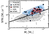 |
Fig. 1. ALMOND and EMPIRE on the star-forming main sequence (SFMS) of galaxies. Grey shows all galaxies from the PHANGS–ALMA survey (Leroy et al. 2021b). Red and blue markers present galaxies from the EMPIRE (Jiménez-Donaire et al. 2019) and ALMOND surveys (Neumann et al. 2023a), respectively, with the same SFR calibration adopted across the merged sample. Contours indicate 25, 50, and 75 percentile areas of the respective samples. The solid black line marks the star-forming main sequence from z0MGS (Leroy et al. 2019). The black squares and crosses indicate the presence of a bar or AGN in the respective galaxy, taken from Table E.1. |
Star formation rate. We estimate the kiloparsec-scale SFR and SFR surface density (ΣSFR) following the methodology of the original ALMOND paper (Neumann et al. 2023a), which used a combination of infrared (IR; 22 μm) maps from Wide-field Infrared Survey Explore (WISE; Wright et al. 2010) and far-ultraviolet (FUV; 154 nm) maps from Galaxy Evolution Explorer (GALEX; Martin et al. 2005). These maps were taken from the z0MGS atlas (Leroy et al. 2019) and converted to SFR following their best FUV+22 μm prescription. Although EMPIRE employed Spitzer and Herschel IR measurements to estimate the SFR, here we adopted the same methodology across EMPIRE and ALMOND, using the FUV+22 μm-based SFR maps for the full sample.
Stellar mass. We estimated the stellar mass surface density (Σ⋆) from Spitzer 3.6 μm observations (Sheth et al. 2010; Querejeta et al. 2021). We used the dust-corrected maps from Querejeta et al. (2015) and adopted a mass-to-light ratio of Υ⋆ = 0.6 M⊙ L .
.
Dynamical equilibrium pressure. The dynamical equilibrium pressure (PDE) expresses the total interstellar pressure needed to support a disc in vertical dynamical equilibrium (e.g. see Ostriker & Kim 2022; Schinnerer & Leroy 2024). We estimated PDE by calculating the weight of the interstellar medium in the galaxy potential via
 (1)
(1)
where Σgas = Σmol + Σatom is the total gas surface density, ρ⋆ is the stellar mass volume density, and σgas,z = 15 km s−1 (e.g. Sun et al. 2018) is the gas velocity dispersion perpendicular to the galactic disc. Computing ρ⋆ required estimates of the stellar scale heights, which were estimated from measured stellar disc scale lengths by assuming a typical disc flattening ratio (see Sun et al. 2020a, 2022, for more details). Estimating PDE additionally required measurements of the atomic gas content, which were taken from H I 21 cm line observations (all with angular resolutions similar to or higher than that of HCN). These observations were available for 26 galaxies of our sample (Table E.1), hence limiting the analysis of PDE relations to those 26 galaxies.
Gao–Solomon relation.
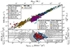 |
Fig. 2. Gao–Solomon relation. SFR (top) and SFR/LHCN (a proxy of SFEdense; bottom) as a function of HCN luminosity across a literature compilation and the ALMOND (blue circles) and EMPIRE (red circles) surveys. Note that we re-calculated the SFR across EMPIRE galaxies using a combination of IR and FUV data (see Sect. 2). Our literature compilation contains HCN observations that include Galactic clumps and clouds (squares), resolved nearby galaxies (circles), and unresolved entire galaxies (diamonds). For more details on the compilation, see Appendix B. The plotted data points show all (3-sigma) detected sightlines. The solid black line shows the median SFR/HCN computed from these data points across all datasets (without duplicates across targets), and the dashed lines mark the 1-sigma scatter (Table 1). The bottom panel shows the ratio SFR/HCN as a function of LHCN, grouping the data into the same subsamples, for which the 10-percentile density contours of the respective subsamples are shown. We plot ALMOND and EMPIRE data separately, and the blue and red contours present the 10-percentile levels of these surveys. |
Conversion factors, molecular gas surface density, and dense gas fraction. We focused on the ratios HCN/CO and SFR/HCN. For reference, we converted them to fiducial physical quantities using fixed conversion factors, αCO ≡ Mmol/LCO ≡ Σmol/WCO and αHCN ≡ Mdense/LHCN ≡ Σdense/WHCN, adopting  (Bolatto et al. 2013) and αHCN 15 M⊙ pc−2 (K km s−1)−1 (Schinnerer & Leroy 2024). Aside from aiming to remain ‘close to the observations’, we did this because the environmental dependence of the HCN-to-dense gas conversion factor, αHCN, remains unclear, with no obvious best prescription and likely significant covariance with αCO (see Usero et al. 2015).
Nevertheless, to leverage recent progress in understanding αCO variations, we employed a variable αCO (hereafter αCOvar) when considering molecular gas surface density, Σmol, or dynamical equilibrium pressure (PDE; see the paragraphs below) as independent variables (i.e. on the x-axis). We calculated
 (2)
(2)
adopting the αCOvar prescription from Schinnerer & Leroy (2024). This αCOvar depends on metallicity and Σ⋆ (see Appendix C for more details on the variable conversion factor and line ratio prescriptions, including references to the works synthesised by Schinnerer & Leroy 2024).
When quoting HCN/CO, we cast our results in terms of CO(1 − 0) and employed the CO(2 − 1)/CO(1 − 0) line ratio calibration as a function of ΣSFR to convert PHANGS–ALMA CO(2 − 1) to CO(1 − 0) intensities (see Appendix C). EMPIRE already has CO(1 − 0) maps.
For both quantities, we provide reference conversions to physical units. We calculated the ‘dense gas fraction’ as the ratio between dense and bulk molecular gas using fixed conversion factors, fdense ≡ Mdense/Mmol ∝ HCN/CO, as
 (3)
(3)
We converted SFR/HCN to an approximate star formation efficiency of dense molecular gas, SFEdense ≡ SFR/Mdense, via
 (4)
(4)
3. Results and discussion
3.1. Gao–Solomon relation
In Fig. 2 we present the ‘Gao–Solomon’ relation (Gao & Solomon 2004), the scaling relationship between SFR and LHCN. We placed ALMOND and EMPIRE in the context of a literature compilation that comprises 31 HCN surveys spanning from the Milky Way to the high-redshift universe. This includes observations of individual cores and molecular clouds within the Milky Way and the Local Group, spatially resolved maps of galaxies, and integrated galaxy data. On the x- and y-axes, we indicate both the observed luminosities (HCN and IR) and the inferred physical quantities (Mdense and SFR), assuming linear conversions with fixed conversion factors αHCN and CIR4. ALMOND and EMPIRE form the largest resolved galaxy dataset, filling in the large gap in spatial scale, SFR, and LHCN between integrated galaxy and individual cloud studies.
In the bottom panel of Fig. 2, the y-axis displays the ratio between SFR and LHCN. Across the full literature sample, we find a median SFR/HCN of 1.3 × 10⁻⁷ M⊙ yr−1 (K km s−1 pc2)−1 with a 1-sigma scatter of 0.52 dex, which is consistent with previous literature compilations (e.g. Jiménez-Donaire et al. 2019; Bešlić et al. 2024). We also computed the respective median SFEdense values and scatter for the individual subsamples: clumps and clouds (squares), resolved galaxy observations (circles), and entire galaxies (diamonds). The values, along with the values specifically for ALMOND and EMPIRE, are listed in Table 1. Overall, the literature compilation demonstrates that the HCN luminosity is a reasonable predictor of the SFR from cloud to galaxy scales across ten orders of magnitude. However, at any given HCN luminosity, there is a significant scatter, σ ∼ 0.5 dex. Moreover, the scatter increases from large (entire galaxy; σ = 0.27 dex) to small scales (clouds; σ = 0.70 dex), suggesting that there are significant variations in SFEdense within galaxies (discussed in Sect. 3.2) that average out at integrated galaxy scales.
SFR/HCN can be interpreted, with significant uncertainty due to the uncertain conversion factor, as the rate per unit mass at which dense molecular gas converts into stars. Across the detected sightlines of the full literature sample, we find a median SFEdense ≈ 8.9 × 10⁻⁹ yr−1, or equivalently a median dense gas depletion time of τdepdense ≈ 112 Myr, indicating that the rate of present-day star formation would consume the available dense gas in this time period. For reference, this is ≈10 times lower than estimates for  , the overall molecular gas depletion time in similar samples (Sun et al. 2023). The star formation efficiency per freefall time, ϵffdense = SFEdense ⋅ tffdense, is of theoretical interest (e.g. Krumholz & McKee 2005; Federrath & Klessen 2012) because it captures the efficiency of star formation relative to the timescale expected for gravitational collapse, and so normalises for density. The freefall time of the dense molecular gas was computed as tffdense = 0.8 Myr, assuming that HCN traces gas above a density of nH2dense ≈ 3 × 103 cm−3 (Jones et al. 2023; Bemis et al. 2024). Across the full literature sample, we obtain a median ϵffdense ≈ 0.7%, which suggests that only 0.7% of the dense molecular gas is converted into stars per gravitational collapse timescale. This demonstrates that even in the dense gas, star formation appears to be an extremely inefficient process.
Dense gas tracer and environment in ALMOND and EMPIRE.
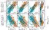 |
Fig. 3. Dense gas relations with kiloparsec-scale environmental conditions. HCN/CO (top), a proxy of fdense, and SFR/HCN (bottom), a proxy of SFEdense, are shown as a function of stellar mass surface density (Σ⋆), molecular gas surface density (Σmol), and dynamical equilibrium pressure (PDE) across 31 galaxies from ALMOND and EMPIRE. The markers denote significant stacked measurements (S/N ≥ 3) across disc (circle) and centre (triangle) spaxels. The downward and upward pointing arrows denote upper (HCN/CO) and lower limits (SFR/HCN). Filled contours show 25, 50, and 75 percentile kernel density estimates. Across centres, we indicate the presence of an AGN (cross). All relations have been fitted with LinMix, taking measurement uncertainties and upper and lower limits into account (parameters in Table 2). The solid black line shows the best-fit line, and the grey-shaded area indicates the 1-sigma scatter of S/N ≥ 3 data. The right panels show violin plots of the HCN/CO and SFR/HCN distribution across the respective samples (disc, centre, centre with an AGN), where the black bar and white markers indicate the 25th to 75th percentile range and the median, respectively, across the S/N ≥ 3 data. The vertical cyan lines in the disc violins mark the median computed from all S/N data. |
3.2. Dense gas relations with environmental conditions
Figure 2 shows significant scatter in SFR/HCN. Previous works have found that both SFR/HCN and HCN/CO depend systematically on environmental factors, including the stellar mass surface density (Σ⋆), the molecular gas mass surface density (Σmol), and the interstellar pressure inferred from dynamical equilibrium (PDE; Usero et al. 2015; Gallagher et al. 2018a; Jiménez-Donaire et al. 2019). The combined ALMOND and EMPIRE samples are ideal for measuring these environmental variations. Individual regions follow the overall Gao–Solomon relation and show a comparable scatter to the full literature sample. The kiloparsec-scale resolution is, on the one hand, high enough to resolve galaxies into discrete regions, including centres, bars, and spiral arms, but is, on the other hand, coarse enough to average over many individual regions to access the time-averaged mean HCN/CO and SFR/HCN.
In Fig. 3 we use ALMOND and EMPIRE to make the most rigorous measurement to date of the scaling relations relating HCN/CO and SFR/HCN to these environmental factors. For each galaxy we spectrally stacked the HCN(1 − 0) and CO(1 − 0) lines in bins of Σ⋆, Σmol, and PDE using PyStacker5. We used the CO data, which have a much higher signal-to-noise ratio than the HCN, to determine the local mean reference velocity for the stacks (see Neumann et al. 2023b, and references therein for details on the spectral stacking methodology; Appendix D presents the spectral stacks of HCN and CO). For bins in which the stacks do not yield 3-sigma HCN detections, we estimated upper limits for HCN/CO and lower limits for SFR/HCN. We fitted the combined set of stacks (including upper limits) for all galaxies using a linear function of the form
 (5)
(5)
where X = {Σ⋆, Σmol, PDE} and Y = {HCN/CO, SFR/HCN} are the x- and y-axis variables, respectively. The slopes and intercepts are denoted as m and b, and x0 = {2.4, 1.4, 5.0} is a value close to the median X value. Centring the fit at x0 minimises the covariance between m and b. The fitting was performed with the linear regression tool LinMix6, which takes measurement uncertainties and 3-sigma upper (lower) limits on HCN/CO (SFR/HCN) into account (see e.g. Neumann et al. 2023a, for more details on the fitting routine). The fit parameters are presented in Table 2. We note that the range of Σ⋆, Σmol, and PDE covered by these results corresponds to the inner, molecular-gas-dominated parts of galaxies, where most stars form.
We find strong correlations between the stacked HCN/CO and all three quantities, and anti-correlations between SFR/HCN and the same quantities (Fig. 3 and Table 2). HCN/CO increases and SFR/HCN decreases with increasing Σ⋆, Σmol, and PDE. The slopes are significant, with both HCN/CO and SFR/HCN changing by ∼1 dex across our sample. ALMOND and EMPIRE have consistent results despite using different telescopes and using different CO lines (see Appendix A).
The enhanced HCN/CO in high-surface-density, high-pressure environments indicates that a deeper gravitational potential and more abundant overall molecular gas lead to the formation of denser molecular clouds. This picture agrees well with the one that has emerged from high-physical-resolution CO imaging, which shows that the mean cloud-scale gas surface density and velocity dispersion correlate with these same environmental factors (Sun et al. 2022). In fact, one of the main results from ALMOND has been a good direct correlation between the cloud-scale gas properties and the density-sensitive HCN/CO line ratio (Neumann et al. 2023a). The fact that spectroscopic (presented here) and CO imaging results show similar trends as a function of galactic environment provides strong evidence that the physical properties of molecular clouds vary as a function of the galactic environment. The HCN/CO variations that we observe are continuous across the whole range of our sample, with a ∼0.2 dex scatter about the correlation.
SFR/HCN anti-correlates with Σ⋆, Σmol, and PDE. This anti-correlation is also significant, though the correlation coefficient is weaker, and the data show more residual scatter in SFR/HCN compared to the trends in HCN/CO. At face value, this indicates that the denser molecular gas that effectively emits HCN is less efficiently converted to stars in high-surface-density, high-pressure parts of galaxies. A popular explanation for this trend has been that HCN-emitting material in these denser environments does not necessarily uniquely correspond to the overdense, self-gravitating parts of clouds that collapse to form stars (e.g. Krumholz & Thompson 2007; Shetty et al. 2014; Gallagher et al. 2018b; Neumann et al. 2023a; Bemis & Wilson 2023; Bemis et al. 2024)
3.3. Dense gas ratios in galaxy centres
The centres of galaxies often exhibit high Σmol, Σ⋆, and PDE; hence, one expects high HCN/CO and low SFR/HCN in galaxy centres compared to the discs. In Fig. 3 we separately indicate galaxy centres in contrast to the rest of the galaxy. For this exercise, we considered the central kiloparsec-scale, beam-size aperture as the centre and refer to the remaining galaxy parts as the disc.
We find that centres typically have high HCN/CO (median of 0.045; see Table E.2) compared to the discs (median of 0.013) that are not consistent within the 1-sigma scatter and low SFR/HCN (median of 7.8 × 10⁻⁸ M⊙ yr−1 pc−2 (K km s−1)−1 compared to the disc median of 1.3 × 10⁻⁷ M⊙ yr−1 pc−2 (K km s−1)−1 (but overlapping 1-sigma intervals). In the following, we base our discussion of the centre-disc comparison on the relations with Σ⋆, which have uncorrelated axes, in contrast to the relations with Σmol and PDE, which depend on the CO line intensity. To first order, centres appear to follow the same average HCN/CO and SFR/HCN against Σ⋆ trend, showing a continuous extension of the disc trends. The higher HCN/CO (lower SFR/HCN) in galaxy centres then simply results from the high Σ⋆ (Σmol, PDE) environment of centres. However, there are some deviations from this simple picture in the SFR/HCN against Σ⋆ relation. On the one hand, the disc measurements in intermediate Σ⋆ environments (Σ⋆ ≈ 2 × 10² M⊙ pc−2 − 1 × 10³ M⊙ pc−2) tend to have low SFR/HCN compared to the average trend, while centres show high SFR/HCN across the same Σ⋆ range. These deviations could be explained via variations with dynamical environments (e.g. Neumann et al. 2024 found a low SFR/HCN in the galactic bar) but remain speculative due to the coarse, kiloparsec-scale resolution of the ALMOND and EMPIRE observations and hence require higher-resolution observations that resolve these morphological regions.
If taken at face value, the low SFEdense in galaxy centres could imply that these environments are typically less efficient at forming stars per unit of dense gas mass, which could be explained by the higher gas turbulence in these environments acting against gravitational collapse (e.g. Usero et al. 2015; Neumann et al. 2023a). However, a similarly likely explanation is that HCN might not be a robust tracer of dense gas in galaxy centres – for example due to increased optical depth, IR pumping (e.g. Matsushita et al. 2015), or electron excitation, (e.g. Goldsmith & Kauffmann 2018) – and potentially trace more of the bulk gas in these high-density regions (see the explanation above). Therefore, we might expect αHCN to vary between disc and centre regions. For instance, if one assumes that αHCN variations are driven by optical depth effects and vary similarly to αCO (Teng et al. 2023; Bemis et al. 2024), αHCN would be lower in galaxy centres and thus yield higher SFEdense that are more comparable to disc values.
One might expect that active galactic nuclei (AGNs) boost HCN emission (e.g. Goldsmith & Kauffmann 2018; Matsushita et al. 2015), deplete gas (e.g. Ellison et al. 2021), or quench star formation (e.g. Nelson et al. 2019). In Fig. 3 we additionally indicate the presence of an AGN (cross; 14 galaxies) for the galaxy centres and show their median and distribution in the right panels. We find that active centres have 50% higher HCN/CO and lower SFRs, though distributions are similar to those found in non-active galaxies and the differences are not significant at the 1-sigma level. The variations in dense gas and star formation in AGN-affected regions are likely not well resolved at the scales probed in this study (∼1 − 2 kpc) and require sub-kiloparsec-resolution observations.
4. Conclusions
We present the resolved 1–2 kpc resolution dense gas tracer scaling relations for ALMA ALMOND, a survey of HCN emission from 25 star-forming disc galaxies. Combining ALMOND with the IRAM 30 m EMPIRE survey, we measured how HCN/CO and SFR/HCN, observational quantities sensitive to the gas density and star formation efficiency of dense gas, depend on the local stellar and molecular gas mass surface density (Σ⋆ and ΣSFR) and the estimated dynamical equilibrium pressure (PDE). Our total sample of 31 resolved galaxies represents a factor of > 3 increase in the number of galaxies compared to the previous state-of-the-art dense gas mapping surveys. HCN/CO correlates with all three environmental measures, showing similar trends to those found for cloud-scale (∼100 pc) CO imaging. Our results support the view that the physical state of molecular gas depends on the galactic environment. SFR/HCN anti-correlates with surface density and PDE, though they show moderately more scatter than the HCN/CO correlations. This reinforces the notion that the scatter in the Gao–Solomon relation is physical in origin and that the relation between any specific dense gas tracer and star formation activity is environment-dependent. While the physical explanations for each of these trends remain subjects of active research, their presence in the data is clear, and ALMA ALMOND + IRAM 30 m EMPIRE provides the best measurement to date in the molecular-gas-dominated, star-forming parts of massive disc galaxies.
Data availability
The HCN and CO data products used in this paper are publicly available via https://www.iram.fr/ILPA/LP015/ (EMPIRE), https://www.canfar.net/storage/list/phangs/RELEASES/ALMOND/ (ALMOND), and https://www.canfar.net/storage/list/phangs/RELEASES/PHANGS-ALMA/ (PHANGS–ALMA). The HCN literature compilation, data products and tables presented in this work are publicly available via https://www.canfar.net/storage/list/phangs/RELEASES/Neumann_etal_2024b/. The Python scripts used to create the data products, figures and tables are available via https://github.com/lukas-neumann-astro/publications/tree/main/Neumann_etal_2024b/.
Eight MIxing Receiver (EMIR) Multiline Probe of the Interstellar medium (ISM) Regulating galaxy Evolution; https://empiresurvey.yourwebsitespace.com
ACA Large-sample Mapping Of Nearby galaxies in Dense gas.
All data here have observed HCN, but for the y-axis we adopted the best-estimate SFR and converted it to the equivalent LIR using a constant IR-to-SFR conversion factor,  (Murphy et al. 2011).
Acknowledgments
We would like to thank the referee, Mark Heyer, for his constructive and concise feedback that helped improve the paper. This work was carried out as part of the PHANGS collaboration. LN acknowledges funding from the Deutsche Forschungsgemeinschaft (DFG, German Research Foundation) – 516405419. AKL gratefully acknowledges support by grants 1653300 and 2205628 from the National Science Foundation, by award JWST-GO-02107.009-A, and by a Humboldt Research Award from the Alexander von Humboldt Foundation. AU acknowledges support from the Spanish grants PGC2018-094671-B-I00, funded by MCIN/AEI/10.13039/501100011033 and by “ERDF A way of making Europe”, and PID2019-108765GB-I00, funded by MCIN/AEI/10.13039/501100011033. RSK acknowledges financial support via the ERC Synergy Grant “ECOGAL” (project ID 855130), via the Heidelberg Cluster of Excellence (EXC 2181 – 390900948) “STRUCTURES”, and via the BMWK project “MAINN” (funding ID 50OO2206). RSK also thanks the 2024/25 Class of Radcliffe Fellows for highly interesting and stimulating discussions. FHL gratefully acknowledges funding from the European Research Council’s starting grant ERC StG-101077573 (“ISM-METALS”). HAP acknowledges support from the National Science and Technology Council of Taiwan under grant 110-2112-M-032-020-MY3. This paper makes use of the following ALMA data, which have been processed as part of the ALMOND and PHANGS–ALMA surveys: ADS/JAO.ALMA#2012.1.00650.S, ADS/JAO.ALMA#2013.1.01161.S, ADS/JAO.ALMA#2015.1.00925.S, ADS/JAO.ALMA#2015.1.00956.S, ADS/JAO.ALMA#2017.1.00230.S, ADS/JAO.ALMA#2017.1.00392.S, ADS/JAO.ALMA#2017.1.00766.S, ADS/JAO.ALMA#2017.1.00815.S, ADS/JAO.ALMA#2017.1.00886.L, ADS/JAO.ALMA#2018.1.01171.S, ADS/JAO.ALMA#2018.1.01651.S, ADS/JAO.ALMA#2018.A.00062.S. ADS/JAO.ALMA#2019.2.00134.S, ADS/JAO.ALMA#2021.1.00740.S, ALMA is a partnership of ESO (representing its member states), NSF (USA), and NINS (Japan), together with NRC (Canada), NSC and ASIAA (Taiwan), and KASI (Republic of Korea), in cooperation with the Republic of Chile. The Joint ALMA Observatory is operated by ESO, AUI/NRAO, and NAOJ. The National Radio Astronomy Observatory (NRAO) is a facility of the National Science Foundation operated under cooperative agreement by Associated Universities, Inc. This work makes use of data products from the Wide-field Infrared Survey Explorer (WISE), which is a joint project of the University of California, Los Angeles, and the Jet Propulsion Laboratory/California Institute of Technology, funded by NASA. This work is based in part on observations made with the Galaxy Evolution Explorer (GALEX). GALEX is a NASA Small Explorer, whose mission was developed in cooperation with the Centre National d’Etudes Spatiales (CNES) of France and the Korean Ministry of Science and Technology. GALEX is operated for NASA by the California Institute of Technology under NASA contract NAS5-98034.
References
- Anand, G. S., Lee, J. C., Van Dyk, S. D., et al. 2021, MNRAS, 501, 3621 [Google Scholar]
- Barnes, A. T., Longmore, S. N., Battersby, C., et al. 2017, MNRAS, 469, 2263 [Google Scholar]
- Bemis, A. R., & Wilson, C. D. 2023, ApJ, 945, 42 [NASA ADS] [CrossRef] [Google Scholar]
- Bemis, A. R., Wilson, C. D., Sharda, P., Roberts, I. D., & He, H. 2024, A&A, 692, A146 [NASA ADS] [CrossRef] [EDP Sciences] [Google Scholar]
- Bešlić, I., Barnes, A. T., Bigiel, F., et al. 2021, MNRAS, 506, 963 [CrossRef] [Google Scholar]
- Bešlić, I., Barnes, A. T., Bigiel, F., et al. 2024, A&A, 689, A122 [NASA ADS] [CrossRef] [EDP Sciences] [Google Scholar]
- Bigiel, F., Leroy, A. K., Blitz, L., et al. 2015, ApJ, 815, 103 [NASA ADS] [CrossRef] [Google Scholar]
- Bigiel, F., Leroy, A. K., Jiménez-Donaire, M. J., et al. 2016, ApJ, 822, L26 [NASA ADS] [CrossRef] [Google Scholar]
- Bolatto, A. D., Wolfire, M., & Leroy, A. K. 2013, ARA&A, 51, 207 [CrossRef] [Google Scholar]
- Braine, J., Shimajiri, Y., André, P., et al. 2017, A&A, 597, A44 [NASA ADS] [CrossRef] [EDP Sciences] [Google Scholar]
- Brouillet, N., Muller, S., Herpin, F., Braine, J., & Jacq, T. 2005, A&A, 429, 153 [NASA ADS] [CrossRef] [EDP Sciences] [Google Scholar]
- Buchbender, C., Kramer, C., Gonzalez-Garcia, M., et al. 2013, A&A, 549, A17 [NASA ADS] [CrossRef] [EDP Sciences] [Google Scholar]
- Chen, H., Gao, Y., Braine, J., & Gu, Q. 2015, ApJ, 810, 140 [NASA ADS] [CrossRef] [Google Scholar]
- Chen, H., Braine, J., Gao, Y., Koda, J., & Gu, Q. 2017, ApJ, 836, 101 [NASA ADS] [CrossRef] [Google Scholar]
- Chin, Y. N., Henkel, C., Whiteoak, J. B., et al. 1997, A&A, 317, 548 [Google Scholar]
- Chin, Y. N., Henkel, C., Millar, T. J., Whiteoak, J. B., & Marx-Zimmer, M. 1998, A&A, 330, 901 [NASA ADS] [Google Scholar]
- Chung, A., van Gorkom, J. H., Kenney, J. D. P., Crowl, H., & Vollmer, B. 2009, AJ, 138, 1741 [Google Scholar]
- Crocker, A., Krips, M., Bureau, M., et al. 2012, MNRAS, 421, 1298 [NASA ADS] [CrossRef] [Google Scholar]
- de Blok, W. J. G., Healy, J., Maccagni, F. M., et al. 2024, A&A, 688, A109 [NASA ADS] [CrossRef] [EDP Sciences] [Google Scholar]
- den Brok, J. S., Chatzigiannakis, D., Bigiel, F., et al. 2021, MNRAS, 504, 3221 [NASA ADS] [CrossRef] [Google Scholar]
- Eibensteiner, C., Barnes, A. T., Bigiel, F., et al. 2022, A&A, 659, A173 [CrossRef] [EDP Sciences] [Google Scholar]
- Eibensteiner, C., Sun, J., Bigiel, F., et al. 2024, A&A, 691, A163 [NASA ADS] [CrossRef] [EDP Sciences] [Google Scholar]
- Ellison, S. L., Wong, T., Sánchez, S. F., et al. 2021, MNRAS, 505, L46 [NASA ADS] [CrossRef] [Google Scholar]
- Evans, N. J., II, Heiderman, A., & Vutisalchavakul, N. 2014, ApJ, 782, 114 [CrossRef] [Google Scholar]
- Federrath, C., & Klessen, R. S. 2012, ApJ, 761, 156 [Google Scholar]
- Gallagher, M. J., Leroy, A. K., Bigiel, F., et al. 2018a, ApJ, 858, 90 [NASA ADS] [CrossRef] [Google Scholar]
- Gallagher, M. J., Leroy, A. K., Bigiel, F., et al. 2018b, ApJ, 868, L38 [CrossRef] [Google Scholar]
- Gao, Y., & Solomon, P. M. 2004, ApJ, 606, 271 [NASA ADS] [CrossRef] [Google Scholar]
- Gao, Y., Carilli, C. L., Solomon, P. M., & Vanden Bout, P. A. 2007, ApJ, 660, L93 [NASA ADS] [CrossRef] [Google Scholar]
- García-Burillo, S., Usero, A., Alonso-Herrero, A., et al. 2012, A&A, 539, A8 [Google Scholar]
- Goldsmith, P., & Kauffmann, J. 2018, Am. Astron. Soc. Meet. Abstr., 231, 130.06 [Google Scholar]
- Graciá-Carpio, J., García-Burillo, S., Planesas, P., Fuente, A., & Usero, A. 2008, A&A, 479, 703 [NASA ADS] [CrossRef] [EDP Sciences] [Google Scholar]
- Herrera-Endoqui, M., Díaz-García, S., Laurikainen, E., & Salo, H. 2015, A&A, 582, A86 [NASA ADS] [CrossRef] [EDP Sciences] [Google Scholar]
- Heyer, M., Gregg, B., Calzetti, D., et al. 2022, ApJ, 930, 170 [NASA ADS] [CrossRef] [Google Scholar]
- Jiménez-Donaire, M. J., Bigiel, F., Leroy, A. K., et al. 2017, MNRAS, 466, 49 [CrossRef] [Google Scholar]
- Jiménez-Donaire, M. J., Bigiel, F., Leroy, A. K., et al. 2019, ApJ, 880, 127 [CrossRef] [Google Scholar]
- Jones, P. A., Burton, M. G., Cunningham, M. R., et al. 2012, MNRAS, 419, 2961 [Google Scholar]
- Jones, G. H., Clark, P. C., Glover, S. C. O., & Hacar, A. 2023, MNRAS, 520, 1005 [NASA ADS] [CrossRef] [Google Scholar]
- Juneau, S., Narayanan, D. T., Moustakas, J., et al. 2009, ApJ, 707, 1217 [NASA ADS] [CrossRef] [Google Scholar]
- Kepley, A. A., Leroy, A. K., Frayer, D., et al. 2014, ApJ, 780, L13 [Google Scholar]
- Krips, M., Neri, R., García-Burillo, S., et al. 2008, ApJ, 677, 262 [NASA ADS] [CrossRef] [Google Scholar]
- Krumholz, M. R., & McKee, C. F. 2005, ApJ, 630, 250 [Google Scholar]
- Krumholz, M. R., & Thompson, T. A. 2007, ApJ, 669, 289 [NASA ADS] [CrossRef] [Google Scholar]
- Lada, C. J., Forbrich, J., Lombardi, M., & Alves, J. F. 2012, ApJ, 745, 190 [NASA ADS] [CrossRef] [Google Scholar]
- Lang, P., Meidt, S. E., Rosolowsky, E., et al. 2020, ApJ, 897, 122 [CrossRef] [Google Scholar]
- Leroy, A. K., Sandstrom, K. M., Lang, D., et al. 2019, ApJS, 244, 24 [Google Scholar]
- Leroy, A. K., Hughes, A., Liu, D., et al. 2021a, ApJS, 255, 19 [NASA ADS] [CrossRef] [Google Scholar]
- Leroy, A. K., Schinnerer, E., Hughes, A., et al. 2021b, ApJS, 257, 43 [NASA ADS] [CrossRef] [Google Scholar]
- Leroy, A. K., Rosolowsky, E., Usero, A., et al. 2022, ApJ, 927, 149 [NASA ADS] [CrossRef] [Google Scholar]
- Lin, L., Pan, H.-A., Ellison, S. L., et al. 2024, ApJ, 963, 115 [NASA ADS] [CrossRef] [Google Scholar]
- Martin, D. C., Fanson, J., Schiminovich, D., et al. 2005, ApJ, 619, L1 [Google Scholar]
- Matsushita, S., Trung, D.-V., Boone, F., et al. 2015, Publ. Korean Astron. Soc., 30, 439 [Google Scholar]
- Murphy, E. J., Condon, J. J., Schinnerer, E., et al. 2011, ApJ, 737, 67 [Google Scholar]
- Nelson, D., Pillepich, A., Springel, V., et al. 2019, MNRAS, 490, 3234 [Google Scholar]
- Neumann, L., Gallagher, M. J., Bigiel, F., et al. 2023a, MNRAS, 521, 3348 [NASA ADS] [CrossRef] [Google Scholar]
- Neumann, L., den Brok, J. S., Bigiel, F., et al. 2023b, A&A, 675, A104 [NASA ADS] [CrossRef] [EDP Sciences] [Google Scholar]
- Neumann, L., Bigiel, F., Barnes, A. T., et al. 2024, A&A, 691, A121 [NASA ADS] [CrossRef] [EDP Sciences] [Google Scholar]
- Ostriker, E. C., & Kim, C.-G. 2022, ApJ, 936, 137 [NASA ADS] [CrossRef] [Google Scholar]
- Privon, G. C., Herrero-Illana, R., Evans, A. S., et al. 2015, ApJ, 814, 39 [CrossRef] [Google Scholar]
- Querejeta, M., Meidt, S. E., Schinnerer, E., et al. 2015, ApJS, 219, 5 [NASA ADS] [CrossRef] [Google Scholar]
- Querejeta, M., Schinnerer, E., Schruba, A., et al. 2019, A&A, 625, A19 [NASA ADS] [CrossRef] [EDP Sciences] [Google Scholar]
- Querejeta, M., Schinnerer, E., Meidt, S., et al. 2021, A&A, 656, A133 [NASA ADS] [CrossRef] [EDP Sciences] [Google Scholar]
- Rybak, M., Hodge, J. A., Greve, T. R., et al. 2022, A&A, 667, A70 [NASA ADS] [CrossRef] [EDP Sciences] [Google Scholar]
- Sánchez, S. F., Rosales-Ortega, F. F., Iglesias-Páramo, J., et al. 2014, A&A, 563, A49 [CrossRef] [EDP Sciences] [Google Scholar]
- Sánchez, S. F., Barrera-Ballesteros, J. K., López-Cobá, C., et al. 2019, MNRAS, 484, 3042 [CrossRef] [Google Scholar]
- Sánchez-García, M., García-Burillo, S., Pereira-Santaella, M., et al. 2022, A&A, 660, A83 [NASA ADS] [CrossRef] [EDP Sciences] [Google Scholar]
- Schinnerer, E., & Leroy, A. K. 2024, ARA&A, 62, 369 [NASA ADS] [CrossRef] [Google Scholar]
- Schinnerer, E., Meidt, S. E., Pety, J., et al. 2013, ApJ, 779, 42 [Google Scholar]
- Sheth, K., Regan, M., Hinz, J. L., et al. 2010, PASP, 122, 1397 [Google Scholar]
- Shetty, R., Clark, P. C., & Klessen, R. S. 2014, MNRAS, 442, 2208 [NASA ADS] [CrossRef] [Google Scholar]
- Stephens, I. W., Jackson, J. M., Whitaker, J. S., et al. 2016, ApJ, 824, 29 [NASA ADS] [CrossRef] [Google Scholar]
- Stuber, S. K., Pety, J., Schinnerer, E., et al. 2023, A&A, 680, L20 [NASA ADS] [CrossRef] [EDP Sciences] [Google Scholar]
- Sun, J., Leroy, A. K., Schruba, A., et al. 2018, ApJ, 860, 172 [NASA ADS] [CrossRef] [Google Scholar]
- Sun, J., Leroy, A. K., Schinnerer, E., et al. 2020a, ApJ, 901, L8 [NASA ADS] [CrossRef] [Google Scholar]
- Sun, J., Leroy, A. K., Ostriker, E. C., et al. 2020b, ApJ, 892, 148 [NASA ADS] [CrossRef] [Google Scholar]
- Sun, J., Leroy, A. K., Rosolowsky, E., et al. 2022, AJ, 164, 43 [NASA ADS] [CrossRef] [Google Scholar]
- Sun, J., Leroy, A. K., Ostriker, E. C., et al. 2023, ApJ, 945, L19 [NASA ADS] [CrossRef] [Google Scholar]
- Tan, Q.-H., Gao, Y., Zhang, Z.-Y., et al. 2018, ApJ, 860, 165 [NASA ADS] [CrossRef] [Google Scholar]
- Teng, Y.-H., Sandstrom, K. M., Sun, J., et al. 2023, ApJ, 950, 119 [NASA ADS] [CrossRef] [Google Scholar]
- Usero, A., Leroy, A. K., Walter, F., et al. 2015, AJ, 150, 115 [Google Scholar]
- Véron-Cetty, M. P., & Véron, P. 2010, A&A, 518, A10 [Google Scholar]
- Walter, F., Brinks, E., de Blok, W. J. G., et al. 2008, AJ, 136, 2563 [Google Scholar]
- Wright, E. L., Eisenhardt, P. R. M., Mainzer, A. K., et al. 2010, AJ, 140, 1868 [Google Scholar]
- Wu, J., Evans, N. J., II, Shirley, Y. L., & Knez, C. 2010, ApJS, 188, 313 [NASA ADS] [CrossRef] [Google Scholar]
Appendix A: EMPIRE versus ALMOND
There are three galaxies (i.e. NGC 628, NGC 2903, NGC 4321) that have been mapped in dense gas tracers (e.g. HCN(1 − 0)) by both surveys, EMPIRE, using the IRAM 30 m, and ALMOND, using the ACA at similar spectral (a few km s−1) and angular resolution (a few tenths of arcseconds) and sensitivity (a few mK). In Figs. A.1 to A.3 we compare the HCN(1 − 0) data from both surveys. We homogenise the two datasets by convolving to the best common spectral (i.e. 10 km s−1) and spatial (i.e. 33″) resolution and re-project to the same half-beam size hexagonal pixel grid.
Figure A.1 shows average HCN(1 − 0) spectra computed across all sightlines within 5 kpc from the galactic centre. We additional overlay CO(2 − 1) average spectra obtained from PHANGS–ALMA (Leroy et al. 2021b), to indicate molecular line emission from a highly significant tracer. This line has been used to infer the velocity-integration window from which we compute HCN(1 − 0) integrated intensities of 41.6 ± 7.3 K km s−1, 39.5 ± 10.7 K km s−1 in NGC 628, 427.8 ± 47.5 K km s−1, 495.7 ± 143.5 K km s−1 in NGC 2903, and 475.0 ± 34.6 K km s−1, 570.2 ± 84.8 K km s−1 in NGC 4321 from ALMOND and EMPIRE, respectively. The average spectra show similar shape and amplitude, demonstrating little to no bias between ALMOND and EMPIRE observations. The integrated line intensities yield consistent values within their uncertainties. The largest deviations are observed at large velocity offsets from the galaxies’ systemic velocities, potentially linked to poor baseline subtraction.
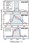 |
Fig. A.1. EMPIRE versus ALMOND: HCN(1 − 0) average spectra. The blue and red lines show average HCN brightness temperatures within rgal ≤ 5 kpc obtained from spatially and spectrally matched ALMOND and EMPIRE observations, respectively, across the three galaxies NGC 628, NGC 2903, NGC 4321 from top to bottom. The grey dashed line shows (homogenised) CO(2 − 1) intensities from PHANGS–ALMA (Leroy et al. 2021b), scaled down by a factor of 20. The grey-shaded area indicates the velocity-integration window constructed using the highly significant CO(2 − 1) data. The resulting integrated intensities are quoted in the text. |
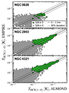 |
Fig. A.2. EMPIRE versus ALMOND: HCN(1 − 0) brightness temperature. Green data points present data, where EMPIRE and ALMOND both yield a 3-sigma detection. Grey data shows low-significant data points. The dashed line marks the 1-to-1 relation, where the dotted lines indicate a ±50 % deviation. |
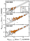 |
Fig. A.3. EMPIRE versus ALMOND: HCN(1 − 0) integrated intensity. Similar to Fig. A.2, but showing the integrated intensities (moment-0) computed across a CO-inferred velocity integration window. Orange and grey points denote data above and below 3-sigma, respectively. |
Figures A.2 and A.3 present a voxel-by-voxel, or pixel-by-pixel comparison between the ALMOND and EMPIRE HCN(1 − 0) brightness temperatures (ppv cube) and integrated intensities (moment-0 map). We find that brightness temperatures and integrated intensities agree well between ALMOND and EMPIRE in all galaxies (deviations ≤50 % across most detected sightlines) and show little bias (≤10 % on average across all data). At lower integrated intensities (≲10−1 K km s−1), EMPIRE yields moderately larger values than ALMOND, which could indicate differences in the calibration and data reduction pipelines.
The comparison between ALMOND and EMPIRE demonstrated that both datasets yield consistent HCN(1 − 0) intensities and subsequent data products. In this work, we employ the ALMOND data for the three galaxies NGC 628, NGC 2903, NGC 4321, due to the slightly better angular resolution and sensitivity of the ALMOND survey.
Figure A4 shows the HCN/CO and SFR/HCN versus Σ⋆, Σmol, and PDE scaling relations across ALMOND (blue hexagons) and EMPIRE (red circles) at kiloparsec resolution. Our best-fit relations are similar, though slightly steeper, to those reported by Jiménez-Donaire et al. (2019) but are now measured for a larger and more diverse sample of galaxies. The steeper slopes have two reasons: a) the ALMOND sample shows steeper trends, and (b) the inclusion of non-detections into the fitting routines yields ∼ 10 % steeper slopes. We observe a larger scatter across the full sample of 31 galaxies compared to the nine EMPIRE galaxies alone, suggesting that the more diverse sample captures a wider range of conditions not captured by the simple scaling relations.
 |
Fig. A.4. Similar to Fig. 3, but separately showing kiloparsec-scale, stacked measurements from ALMOND (blue hexagons) and EMPIRE (red circles). The best-fit line (solid black line) and the corresponding 1-sigma scatter (grey-shaded area) are computed from the combined data using LinMix. |
Appendix B: Dense gas literature
In Fig. 2 we present a literature compilation of HCN surveys from local parsec scale over resolved, kiloparsec scale, to unresolved, entire galaxy observations. The cloud- and clump-scale measurements are taken from observations within the Milky Way (Wu et al. 2010; Lada et al. 2012; Evans et al. 2014; Stephens et al. 2016), the CMZ (Jones et al. 2012; Barnes et al. 2017), and the Local Group, namely the Large and Small Magellanic Clouds (LMC, SMC) (Chin et al. 1997, 1998), M31 (Brouillet et al. 2005), M33 (Buchbender et al. 2013), and low-metallicity local group galaxies (Braine et al. 2017). Resolved galaxy observations, typically from nearby galaxies at 100 pc to 2 kiloparsec scales, include M82 (Kepley et al. 2014), M51 (Usero et al. 2015; Chen et al. 2017; Querejeta et al. 2019; Stuber et al. 2023), NGC 4038/39 (Bigiel et al. 2015), NGC 3351, NGC 3627, NGC 4254, NGC 4321, NGC 5194 (Gallagher et al. 2018a), NGC 3627 (Bešlić et al. 2021), NGC 1068 (Sánchez-García et al. 2022), NGC 6946 (Eibensteiner et al. 2022), NGC 4321 (Neumann et al. 2024), NGC 253 (Bešlić et al. 2024), and the two larger-sample surveys EMPIRE (nine galaxies; Jiménez-Donaire et al. 2019) and ALMOND (25 galaxies; Neumann et al. 2023a). Integrated-galaxy data cover Luminous Infrared Galaxies (LIRGs), Ultra-Luminous Infrared Galaxies (ULIRG), and AGN galaxies (Krips et al. 2008; Graciá-Carpio et al. 2008; Juneau et al. 2009; García-Burillo et al. 2012; Privon et al. 2015), early-type galaxies (Crocker et al. 2012), and high-redshift galaxies (Gao et al. 2007; Rybak et al. 2022).
Appendix C: Conversion factors
For EMPIRE, we use the CO(1 − 0) maps obtained as part of the survey. For ALMOND, we use PHANGS–ALMA CO(2 − 1) maps, which we convert to an equivalent CO(1 − 0) intensity before applying αCO. To do this, we estimate a line ratio, R21, based on the local SFR surface density (ΣSFR) following den Brok et al. (2021), Leroy et al. (2022), and Schinnerer & Leroy (2024):
 (C.1)
(C.1)
with minimum R21 of 0.35 and maximum 1.0. Then we scale the CO(2 − 1) intensity by  to present our results in terms of CO(1 − 0) intensity.
To compute Σmol and PDE, we adopt the variable αCO prescription from Schinnerer & Leroy (2024, their Table 1), which accounts for variations with metallicity (Z; Z⊙ is the solar metallicity) and stellar mass surface density (Σ⋆):
 (C.2)
(C.2)
Stellar mass maps are inferred from Spitzer 3.6 μm observations as explained in Sect. 2. Metallicities are estimated based on simple scaling relations, following Sun et al. (2020b). These use a global mass-metallicity relation (Sánchez et al. 2019) and employ a radial metallicity relation with a fixed gradient of –0.1 dex normalised by the effective radius of each galaxy (Sánchez et al. 2014).
Appendix D: Spectral stacking of HCN and CO
We compute spectral stacks of HCN(1 − 0) and CO(1 − 0) line emission in bins of stellar mass surface density, Σ⋆, molecular gas surface density, Σmol, and dynamical equilibrium pressure, PDE, across the merged sample of 31 galaxies studied in this work. For the ALMOND sample, the CO(2 − 1) intensities from PHANGS–ALMA are first converted into CO(1 − 0) intensities using the line ratio calibration from Sect. C. We note, however, that this has no effect on the stacking procedure. We stack in logarithmic bins for each galaxy individually, selecting ten bins from a fixed minimum (Σ⋆ = 3 × 101 M⊙ pc−2, Σmol = 5 M⊙ pc−2, PDE = 1 × 104 kB K cm−3) to the maximum value of each galaxy. For the centres versus disc HCN scaling relations (Fig. 3), we exclude the centres from the stacking and stacks across the remaining sightlines adopting nine bins. Figure D2 shows exemplary spectral stacks of HCN(1 − 0) and CO(1 − 0) as a function of Σ⋆ across the galaxy NGC 4321.
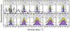 |
Fig. D.1. Spectral stacks of CO (olive) and HCN (purple) across NGC 4321 in logarithmically-spaced bins of Σ⋆. The grey-shaded area indicates the velocity-integration window applied to compute the integrated intensities of the stacked spectra. The labelled boxes show the peak intensity and S/N of the integrated intensities of CO and HCN, respectively, for each stacked spectrum. |
Appendix E: Additional tables
Table E.1 presents the combined galaxy sample composed of 31 galaxies from the EMPIRE and ALMOND surveys, along with their coordinates and global properties.
Galaxy sample (EMPIRE + ALMOND).
Table E.2 lists percentile and median HCN/CO and SFR/HCN values for centre and discs environments discussed in Sect. 3.3.
Galaxy centres vs discs.
All Tables
All Figures
|
Fig. 1. ALMOND and EMPIRE on the star-forming main sequence (SFMS) of galaxies. Grey shows all galaxies from the PHANGS–ALMA survey (Leroy et al. 2021b). Red and blue markers present galaxies from the EMPIRE (Jiménez-Donaire et al. 2019) and ALMOND surveys (Neumann et al. 2023a), respectively, with the same SFR calibration adopted across the merged sample. Contours indicate 25, 50, and 75 percentile areas of the respective samples. The solid black line marks the star-forming main sequence from z0MGS (Leroy et al. 2019). The black squares and crosses indicate the presence of a bar or AGN in the respective galaxy, taken from Table E.1. |
| In the text | |
|
Fig. 2. Gao–Solomon relation. SFR (top) and SFR/LHCN (a proxy of SFEdense; bottom) as a function of HCN luminosity across a literature compilation and the ALMOND (blue circles) and EMPIRE (red circles) surveys. Note that we re-calculated the SFR across EMPIRE galaxies using a combination of IR and FUV data (see Sect. 2). Our literature compilation contains HCN observations that include Galactic clumps and clouds (squares), resolved nearby galaxies (circles), and unresolved entire galaxies (diamonds). For more details on the compilation, see Appendix B. The plotted data points show all (3-sigma) detected sightlines. The solid black line shows the median SFR/HCN computed from these data points across all datasets (without duplicates across targets), and the dashed lines mark the 1-sigma scatter (Table 1). The bottom panel shows the ratio SFR/HCN as a function of LHCN, grouping the data into the same subsamples, for which the 10-percentile density contours of the respective subsamples are shown. We plot ALMOND and EMPIRE data separately, and the blue and red contours present the 10-percentile levels of these surveys. |
| In the text | |
|
Fig. 3. Dense gas relations with kiloparsec-scale environmental conditions. HCN/CO (top), a proxy of fdense, and SFR/HCN (bottom), a proxy of SFEdense, are shown as a function of stellar mass surface density (Σ⋆), molecular gas surface density (Σmol), and dynamical equilibrium pressure (PDE) across 31 galaxies from ALMOND and EMPIRE. The markers denote significant stacked measurements (S/N ≥ 3) across disc (circle) and centre (triangle) spaxels. The downward and upward pointing arrows denote upper (HCN/CO) and lower limits (SFR/HCN). Filled contours show 25, 50, and 75 percentile kernel density estimates. Across centres, we indicate the presence of an AGN (cross). All relations have been fitted with LinMix, taking measurement uncertainties and upper and lower limits into account (parameters in Table 2). The solid black line shows the best-fit line, and the grey-shaded area indicates the 1-sigma scatter of S/N ≥ 3 data. The right panels show violin plots of the HCN/CO and SFR/HCN distribution across the respective samples (disc, centre, centre with an AGN), where the black bar and white markers indicate the 25th to 75th percentile range and the median, respectively, across the S/N ≥ 3 data. The vertical cyan lines in the disc violins mark the median computed from all S/N data. |
| In the text | |
|
Fig. A.1. EMPIRE versus ALMOND: HCN(1 − 0) average spectra. The blue and red lines show average HCN brightness temperatures within rgal ≤ 5 kpc obtained from spatially and spectrally matched ALMOND and EMPIRE observations, respectively, across the three galaxies NGC 628, NGC 2903, NGC 4321 from top to bottom. The grey dashed line shows (homogenised) CO(2 − 1) intensities from PHANGS–ALMA (Leroy et al. 2021b), scaled down by a factor of 20. The grey-shaded area indicates the velocity-integration window constructed using the highly significant CO(2 − 1) data. The resulting integrated intensities are quoted in the text. |
| In the text | |
|
Fig. A.2. EMPIRE versus ALMOND: HCN(1 − 0) brightness temperature. Green data points present data, where EMPIRE and ALMOND both yield a 3-sigma detection. Grey data shows low-significant data points. The dashed line marks the 1-to-1 relation, where the dotted lines indicate a ±50 % deviation. |
| In the text | |
|
Fig. A.3. EMPIRE versus ALMOND: HCN(1 − 0) integrated intensity. Similar to Fig. A.2, but showing the integrated intensities (moment-0) computed across a CO-inferred velocity integration window. Orange and grey points denote data above and below 3-sigma, respectively. |
| In the text | |
|
Fig. A.4. Similar to Fig. 3, but separately showing kiloparsec-scale, stacked measurements from ALMOND (blue hexagons) and EMPIRE (red circles). The best-fit line (solid black line) and the corresponding 1-sigma scatter (grey-shaded area) are computed from the combined data using LinMix. |
| In the text | |
|
Fig. D.1. Spectral stacks of CO (olive) and HCN (purple) across NGC 4321 in logarithmically-spaced bins of Σ⋆. The grey-shaded area indicates the velocity-integration window applied to compute the integrated intensities of the stacked spectra. The labelled boxes show the peak intensity and S/N of the integrated intensities of CO and HCN, respectively, for each stacked spectrum. |
| In the text | |
Current usage metrics show cumulative count of Article Views (full-text article views including HTML views, PDF and ePub downloads, according to the available data) and Abstracts Views on Vision4Press platform.
Data correspond to usage on the plateform after 2015. The current usage metrics is available 48-96 hours after online publication and is updated daily on week days.
Initial download of the metrics may take a while.