| Issue |
A&A
Volume 689, September 2024
|
|
|---|---|---|
| Article Number | A122 | |
| Number of page(s) | 19 | |
| Section | Extragalactic astronomy | |
| DOI | https://doi.org/10.1051/0004-6361/202347568 | |
| Published online | 06 September 2024 | |
The properties and kinematics of HCN emission across the closest starburst galaxy NGC 253 observed with ALMA
1
Argelander-Institut für Astronomie, Universität Bonn, Auf dem Hügel 71, 53121 Bonn, Germany
2
LERMA, Observatoire de Paris, PSL Research University, CNRS, Sorbonne Universités, 75014 Paris, France
3
European Southern Observatory (ESO), Karl-Schwarzschild-Straße 2, 85748 Garching, Germany
4
Observatorio Astronómico Nacional (IGN), C/Alfonso XII, 3, 28014 Madrid, Spain
5
Centro de Desarrollos Tecnológicos, Observatorio de Yebes (IGN), 19141 Yebes, Guadalajara, Spain
6
Astrophysics Research Institute, Liverpool John Moores University, 146 Brownlow Hill, Liverpool L3 5RF, UK
7
Department of Physics, University of Connecticut, Storrs, CT 06269, USA
8
Department of Astronomy, The Ohio State University, 140 West 18th Ave, Columbus, OH 43210, USA
9
Department of Physics, University of Alberta, Edmonton, AB T6G 2E1, Canada
10
Center for Astrophysics, Harvard & Smithsonian, 60 Garden St., 02138 Cambridge, MA, USA
11
Universität Heidelberg, Zentrum für Astronomie, Institut für Theoretische Astrophysik, Albert-Ueberle-Str. 2, 69120 Heidelberg, Germany
12
Research School of Astronomy and Astrophysics, Australian National University, Canberra, ACT 2611, Australia
13
ARC Centre of Excellence for All Sky Astrophysics in 3 Dimensions (ASTRO 3D), Australia
14
Universität Heidelberg, Zentrum für Astronomie, Institut für Theoretische Astrophysik, Albert-Ueberle-Strasse 2, 69120 Heidelberg, Germany
15
Universität Heidelberg, Interdisziplinäres Zentrum für Wissenschaftliches Rechnen, Im Neuenheimer Feld 225, 69120 Heidelberg, Germany
16
Technical University of Munich, School of Engineering and Design, Department of Aerospace and Geodesy, Chair of Remote Sensing Technology, Arcisstr. 21, 80333 Munich, Germany
17
Sterrenkundig Observatorium, Universiteit Gent, Krijgslaan 281 S9, 9000 Gent, Belgium
18
Max Planck Institute for Astronomy, Königstuhl 17, 69117 Heidelberg, Germany
19
Department of Physics, Tamkang University, No. 151, Yingzhuan Road, Tamsui District, New Taipei City 251301, Taiwan
20
Sub-department of Astrophysics, Department of Physics, University of Oxford, Keble Road, Oxford OX1 3RH, UK
Received:
26
July
2023
Accepted:
29
February
2024
Abstract
Context. Investigating molecular gas tracers, such as hydrogen cyanide (HCN), to probe higher densities than CO emission across nearby galaxies remains challenging. This is due to the large observing times required to detect HCN at a high sensitivity and spatial resolution. Although approximate kiloparsec scales of HCN maps are available for tens of galaxies, higher-resolution maps still need to be available.
Aims. We aim to study the properties of molecular gas, the contrast in intensity between two tracers that probe different density regimes (the HCN(1–0)/CO(2–1) ratio), and their kinematics across NGC 253, one of the closest starburst galaxies. With its advanced capabilities, the Atacama Large Millimeter/submillimeter Array (ALMA) can map these features at a high resolution across a large field of view and uncover the nature of such dense gas in extragalactic systems.
Methods. We present new ALMA Atacama Compact Array and Total Power (ACA+TP) observations of the HCN emission across NGC 253. The observations cover the inner 8.6′ of the galaxy disk at a spatial resolution of 300 pc. Our study examines the distribution and kinematics of the HCN-traced gas and its relationship with the bulk molecular gas traced by CO(2–1). We analyze the integrated intensity and mean velocity of HCN and CO along each line of sight. We also used the SCOUSE software to perform spectral decomposition, which considers each velocity component separately.
Results. We find that the denser molecular gas traced by HCN piles up in a ring-like structure at a radius of 2 kpc. The HCN emission is enhanced by two orders of magnitude in the central 2 kpc regions, beyond which its intensity decreases with increasing galactocentric distance. The number of components in the HCN spectra shows a robust environmental dependence, with multiple velocity features across the center and bar. The HCN spectra exhibit multiple velocity features across the center and bar, which shows a robust environmental dependence. We have identified an increase in the HCN/CO ratio in these regions, corresponding to a velocity component likely associated with a molecular outflow. We have also discovered that the ratio between the total infrared luminosity and dense gas mass, which is an indicator of the star formation efficiency of dense gas, is anticorrelated with the molecular gas surface density up to approximately 200 M⊙ pc−2. However, beyond this point, the ratio starts to increase.
Conclusions. We argue that using information about spectroscopic features of molecular emission is an important aspect of understanding molecular properties in galaxies.
Key words: stars: formation / ISM: molecules / galaxies: starburst / radio lines: ISM
Corresponding author; This email address is being protected from spambots. You need JavaScript enabled to view it. .
© The Authors 2024
 Open Access article, published by EDP Sciences, under the terms of the Creative Commons Attribution License (https://creativecommons.org/licenses/by/4.0), which permits unrestricted use, distribution, and reproduction in any medium, provided the original work is properly cited.
This article is published in open access under the Subscribe to Open model. This email address is being protected from spambots. You need JavaScript enabled to view it. to support open access publication.
1. Introduction
The densest structures of molecular clouds are found to be sites of star formation across galaxies (Gao & Solomon 2004; Lada et al. 2012; Longmore et al. 2014). However, since the primary constituent of molecular gas, H2, does not probe the coldest, densest parts of these clouds, other molecular lines are needed to observe star-forming gas and can be used to constrain various properties. In the past, researchers have primarily used CO, the second most abundant molecule in the universe, to observe molecular clouds (see review Bolatto et al. 2013). CO emits relatively bright signals within the millimeter and (sub)millimeter regime, and its abundance scales with H2. The assumption that the CO emission traces the overall molecular gas content of the interstellar medium (ISM) is commonly used within the literature (for example, Bigiel et al. 2008; Leroy et al. 2008; Tacconi 2010; Schruba et al. 2011; Cormier et al. 2014; Genzel et al. 2015; Saintonge et al. 2017).
In most cases, the low-J CO lines can estimate the total H2 mass. However, they might not be reliable bulk tracers in extreme environments with, for example, high cosmic-ray ionization rates (Bisbas et al. 2015) or with intense UV radiation and low metallicity (Pak et al. 1998).
CO is a good tracer of the cloud-scale surface density (Sun et al. 2018), but it does not reveal information about the star-forming part of molecular clouds. Therefore, to probe such dense regions (n > 103 cm−3, 200 M⊙ pc−2), astronomers observe molecular lines with high critical densities (high-critical density molecules; Shirley 2015), such as those of HCN, HCO+, and N2H+, defined in this paper as “dense gas tracers.” However, observing this gas at extragalactic distances is challenging; many preferred molecular lines commonly used in Galactic studies (Forbrich et al. 2014; Pety et al. 2017; Kauffmann et al. 2017), such as N2H+, can only be easily detected toward the centers of bright, nearby galaxies NGC 253 (Martín et al. 2021) and NGC 6946 (Eibensteiner et al. 2022; Jiménez-Donaire et al. 2023).
The J = 1 → 0 transition of the hydrogen cyanide, HCN, is one of the brightest high-critical density molecular lines commonly studied within the extragalactic literature (for instance, Gao & Solomon 2004; Usero et al. 2015; Gallagher et al. 2018b; Jiménez-Donaire et al. 2019; Bešlić et al. 2021; Sánchez-García et al. 2022). The comparison between low- and high-critical density lines, such as CO(1–0) and HCN(1–0), yields an approximate gauge of the intensity contrast between two tracers probing different density regimes, as the latter requires significantly higher densities for collisional excitation compared to the low-J CO lines (ncrit, eff > 104 cm−3 versus > 102 cm−3 – Shirley 2015). This contrast offers the best currently available observational constraint on changes in the underlying density distribution in other galaxies (for example, Leroy et al. 2017b).
From the observational point of view, HCN surveys in extragalactic systems found a tight and linear correlation between the HCN luminosity and star formation rate (SFR, Gao & Solomon 2004; Jiménez-Donaire et al. 2019). This correlation is approximately linear in logarithmic space, spanning more than ten orders of magnitude, and covers a wide range of physical scales: from dense clumps and cores (a few parsecs; see Wu et al. 2010) within the Milky Way, to galaxy disks and galaxy centers (for example, Gao & Solomon 2004; Graciá-Carpio et al. 2008). Although it has been argued that the linear relation between HCN and SFR suggests that gas above a specific density threshold starts forming stars (Lada et al. 2012), systemic variations in the IR/HCN ratio imply that not all dense gas is equally efficient. For example, the central molecular zone (CMZ), known to be the inner 500 pc region of our Galaxy, shows an order of magnitude lower SFR than those predicted from measurements of dense molecular gas (Longmore et al. 2013; Henshaw et al. 2023), implying a possibility of the non-universality of the star formation efficiency (Mac Low & Klessen 2004; Padoan & Nordlund 2011; Federrath & Klessen 2012; Kruijssen et al. 2014; Semenov et al. 2016). This environmental impact on the dense gas’s ability for star formation has also been observed across other galaxies. While most dense gas mass is found in centers of galaxies, this gas is less efficient at star formation than the gas in the rest of the disk (Gallagher et al. 2018b; Jiménez-Donaire et al. 2019). Observed variations in IR/HCN could be caused by non-steady effects dominant at small spatial scales, such as stellar feedback and galactic shear, which become averaged out on larger scales.
In order to fully understand the star formation process, it is important to connect what we learn from studying extragalactic sources with studies of individual star-forming regions within our own Milky Way. To do this, we need to observe molecular clouds in extragalactic samples at a high sensitivity and on small spatial scales while also covering a broad range of different environments and physical conditions. This is a crucial step toward connecting studies of the Milky Way, where we can examine the substructure of individual molecular clouds (Pety et al. 2017), with studies of more distant galaxies that contain vastly different environments, such as starburst galaxies (García-Burillo et al. 2012). To achieve this, observing nearby galaxies spanning the range of scales needed to benchmark our understanding of local clouds and high-z galaxies is essential. Due to their proximity, we can map dense molecular gas content across nearby galaxies at a high spatial resolution and sensitivity. Moreover, the high molecular surface brightness of these sources, known as Σmol, can provide a sensitive mapping of the HCN emission that we can now observe using advanced observing facilities such as ALMA. Recent studies of HCN at higher resolutions, approaching molecular cloud scales of around 100 pc, have been mainly focused on the brightest regions of nearby galaxies, such as in M 51 (Querejeta et al. 2019), a larger part of the disk of NGC 3627 (Bešlić et al. 2021), the center of NGC 6946 (Eibensteiner et al. 2022), and the inner ring of NGC 1068 (Sánchez-García et al. 2022).
In this paper, we answer some of the science questions related to high-critical density molecular emission, such as the following:
-
Distribution of dense molecular gas across NGC 253 (Section 3).
-
The kinematics of the HCN-tracing gas, and its comparison with the CO emission (Section 4).
-
The role of dense gas in star formation processes across different environments found in NGC 253 (Section 5).
To address these questions, we use ALMA observations of the closest starburst galaxy outside the Local Group, the Sculptor galaxy, NGC 253. The main properties of this galaxy are listed in Table 1. NGC 253 (see its composite image in Figure 1) is the highly inclined, starburst galaxy (Rieke et al. 1980) located in the southern hemisphere. Due to its proximity (1 arcsecond corresponds to 17 pc at a distance of 3.7 Mpc; Anand et al. 2021), NGC 253 represents an ideal target for high-resolution studies to understand the nature of its kiloparsec nuclear region (Bolatto et al. 2013; Leroy et al. 2015; Walter et al. 2017; Holdship et al. 2021) of which the center appears to be undergoing an intense phase of active star formation. The star formation rate within the center is SFR = 2 M⊙ yr−1 (Leroy et al. 2015), which is 50% of the SFR found in the whole disk of this galaxy (Sanders et al. 2003).
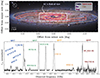 |
Fig. 1. Composite image of NGC 253, its environments, and the 86–101 GHz spectrum taken with ALMA ACA. Top panel: NGC 253 composite (RGB and Hα) image (credits: Terry Robinson). The overlaid dashed gray rectangle shows the total u − υ coverage consisting of 25 pointing mosaic obtained by the ACA 7-m for this work. We indicate dynamical environments present in the disk of NGC 253: the center, bar, ring, and spiral arms (Querejeta et al. 2021). Bottom panel: observed spectrum taken toward the center of NGC 253. Our observations cover frequencies from 85.7 to 101.5 GHz. The term spectral window i (i takes values from 1 to 4) is abbreviated as spwi, and we mark all detected molecular emission lines. |
Main properties of NGC 253.
The central 1 kpc of NGC 253 shows rich molecular emission (see our detected molecular lines in the bottom panel of Figure 1), demonstrated in Martín et al. (2006), Aladro et al. (2011), and Meier et al. (2015), who detected 50 molecular species at a 3 mm wavelength (including, C2H5OH, HOCN, and HC3H). In addition, Atacama Large Millimeter/submillimeter Array (ALMA) Comprehensive High-resolution Extragalactic Molecular Inventory (ALCHEMI) mapped a continuous frequency range from (sub)millimeter to millimeter wavelengths in the nuclear region of NGC 253 (Martín et al. 2021). NGC 253 has a plethora of ancillary data covering a variety of gas phases, from hot (Lopez et al. 2023), atomic (Heckman et al. 2000), molecular (Houghton et al. 1997; Mauersberger et al. 1996; Paglione et al. 2004), and the most recent ACA observations of CO(2–1) which we use in this work (Faesi, in prep.), to ionized gas (Arnaboldi et al. 1995).
Although NGC 253 has been well studied over the last few decades, most investigations have focused on its inner 1–2 kpc nuclear region. The molecular gas outside the galaxy center needs to be better understood, particularly the properties of its dense phase and its kinematics on larger scales in a wide range of disk environments.
In this paper, we present new ACA observations across the disk of the NGC 253. These data have a spatial resolution of 300 pc, covering a large part of the disk of this galaxy (8 × 3′2) and probe different dynamical features in this galaxy. The paper is structured as follows. Section 2 describes observations, data reduction, additional datasets used throughout this work, and present moment maps of the HCN and CO(2–1). Next, we present our results: Section 3 describes the distribution of the line-of-sight HCN emission and the measured HCN/CO(2–1) ratio. Section 4 presents the decomposed line-of-sight HCN emission and the measured properties of such decomposed emission and describes the results of measured velocity dispersion. Moreover, we answer Question 3 in Section 5. Our findings are discussed in Section 6. Finally, we summarize and outline our most important results in Section 7.
2. Observations and data reduction
2.1. ALMA+ACA observations
The observations (project ID: 2019.2.00236.S) of NGC 253 presented in this paper are part of the ALMA Cycle 7 and were obtained in December 2019 and January 2020. We observed molecular line emission using the Atacama Compact Array (7 m – ACA), which included the Total Power (TP) array in Band 3 (84–116 GHz), covering several ”typical” extragalactic tracers of high-density gas, shown on the bottom panel in Figure 1. The total observing time is 22.9 and 44.1 h for the 7 m array and the TP antennas, respectively. The observed field of view contains 25 7 m pointings with the primary beam full-width half maximum (FWHM) of 57.6″, which covers a 114″ × 516″(∼2 × 9 kpc2) region of the inner disk of NGC 253 (see Figure 1). The beam size is 21.40″ × 10.36″, and the beam position angle is 83.5 deg. From our ancillary CO(2–1) observations (Section 2.3) and SFR images (Section 2.4), we find that the region mapped within the ACA comprises 90% of the total molecular mass of NGC 253 and 85% of its total SFR. Thus, our observations cover the brightest regions in molecular gas and the most star-forming parts in NGC 253.
Our interferometric observations are sensitive to the emission from angular scales of ∼14″ (∼240 pc) to the largest angular scale obtained by the TP of ∼100″ (∼1.7 kpc). The obtained sensitivity is ∼2.5 mK (7.6 mJy beam−1) at the angular and spectral resolution of 22″ and 10 km s−1. The spectral setup consisted of four spectral windows with ∼1.8 GHz width and 0.4 MHz resolution laid out as at the bottom of Figure 1. We detected 13 molecular lines, but here, we focus on the HCN(1–0) line covered by spectral window 2, labeled as spw2 on Figure 1.
The raw data calibration was done in Common Astronomy Software Applications (CASA – McMullin et al. 2007), version 6.5, and the imaging and post-processing, including short-spacing correction using the PHANGS-ALMA processing pipeline (Leroy et al. 2021a). Firstly, we flagged all of the emission lines within each band to calculate and subtract the continuum emission. The 7 m data was imaged using CASA’s standard TCLEAN procedure. We used the CO(2–1)-based clean mask (Leroy et al. 2021a,b) as the initial clean mask for our imaging, which was then combined with the single-scale clean during the imaging. The HCN 7m flux within the cleaning mask is 99% of the total flux within the full image.
The single-dish data were also processed using the PHANGS-ALMA total power processing pipeline (Herrera et al. 2020), included in the PHANGS-ALMA pipeline (Leroy et al. 2021a). In the final data reduction step, we combined 7m observations with TP for the missing short-scale emission using the standard CASA task feather. The total flux from the interferometric data is 70% of the total flux measured from the single-dish data. The final data cube was additionally primary beam corrected and convolved to have a circular beam size of 22″ (∼370 pc) and a channel width of 10 km/s.
In addition, we computed the dense gas mass, Mdense, assuming a constant XHCN = 10 [M⊙ (K km s−1 pc2)−1] conversion factor (Gao & Solomon 2004):
![Mathematical equation: $$ \begin{aligned} M_{\rm dense} [\mathrm{M_{\odot }}] = X_{\rm HCN}\cdot L_{\rm HCN} \cdot \cos {i}, \end{aligned} $$](/articles/aa/full_html/2024/09/aa47568-23/aa47568-23-eq1.gif) (1)
(1)
where i is the galaxy inclination reported in Table 1.
2.2. Environmental masks
To separate regions with different characteristics in NGC 253, we used environmental masks defined for this galaxy based on infrared data (Querejeta et al. 2021). They have four regions: the disk, ring, bar, and center. Additionally, NGC 253 has two spiral arm features, visible in optical data (Pence 1980) and constrained from the 3.6 and 4.5 μm observations obtained by the Spitzer telescope, as part of the S4G survey (Muñoz-Mateos et al. 2015; Herrera-Endoqui et al. 2015). Therefore, we also defined a spiral arm mask in this work. We used the unsharp-masked near-infrared Herschel PACS 70 μm data to locate spiral features, and then we fitted those in polar (ρ, θ) space as linear functions. The width of such constructed spiral arms is defined manually in the SAO-NASA ds9 software (Joye & Mandel 2003). Finally, we added these spiral arm regions to the existing environmental mask, shown in Figure 1. We distinguish five environments in NGC 253: the nuclear region lies within the inner ∼0.5 kpc region, and the bar feature is located in the inner two kpc region. The ring is at radii between 2 and 5 kpc, and the dust lanes are at rgal = 5 kpc. All remaining pixels not assigned to any of these environments belong to the disk.
2.3. ALMA-CO(2–1) observations from PHANGS
In this work, we used ancillary ALMA ACA+TP CO(2–1) observations (PI: C. Faesi, 2018.1.01321.S), included in the PHANGS-ALMA survey (PI: E. Schinnerer – Leroy et al. 2021b; Faesi, in prep.). The angular resolution of these data is 8″, and the channel width is 2.5 km s−1. In the final step, we convolved the CO(2–1) data cube to match the working angular and spectral resolution of 22″ and 10 km/s and regrid to a common pixel scale. We computed the molecular surface density using the following equation:
![Mathematical equation: $$ \begin{aligned} \Sigma _{\rm mol} [\mathrm{M_{\odot }\,pc^{-2} }] = \alpha _{\rm CO}\cdot \dfrac{I_{\rm CO(2-1)}}{R_{\rm 21}} \cdot \cos {i} = \alpha _{\rm CO}\cdot \dfrac{I_{\rm CO(2-1)}}{\Sigma _{\mathrm{SFR}}^{0.15}} \cdot \cos {i} , \end{aligned} $$](/articles/aa/full_html/2024/09/aa47568-23/aa47568-23-eq2.gif) (2)
(2)
where αCO is the metallicity-dependent conversion factor taken from Sun et al. (2020), ICO(2 − 1) is the CO(2–1) integrated intensity, R21 is the CO(2–1)/CO(1–0) line ratio (for example, Sandstrom et al. 2013; den Brok et al. 2021; Yajima et al. 2021; Leroy et al. 2022), and i is the same as in Equation (1). In this work, we used the scaling relation:  (see Sun et al. 2023, and references therein). The αCO has a range from 4.2 (at the center) to 20 [M⊙/(K km s−1 pc2)] (at the outskirts). The validity of the αCO factor depends on the mass scales probed. For masses greater than 105 M⊙, the statistical assumptions underlying the αCO factor remain valid (Dickman et al. 1986), which is achieved in our work. We present the Σmol map in Figure A.1.
2.4. Star formation rate
To estimate the star formation rate surface density (ΣSFR), we used a combination of IR Herschel data from the KINGFISH (Key Insights on Nearby Galaxies: a Far-Infrared Survey with Herschel) survey (Kennicutt et al. 2011). To compare our results with recent similar studies (Jiménez-Donaire et al. 2019), we chose to calculate ΣSFR using Herschel bands at λ = 70, 160, and 250 microns. First, we convolved our Herschel maps to a final resolution of 22″ using the kernels defined in Aniano et al. (2011) and matched the coordinate grid with the final HCN data image. We calculated the total infrared surface density (ΣTIR) following the prescription from Galametz et al. (2013):
![Mathematical equation: $$ \begin{aligned} \Sigma _{\rm TIR} [\mathrm{W\,kpc^{-2}}] = \sum _{j} c_{j}\cdot \Sigma _{j} [\mathrm{W\,kpc^{-2}}], \end{aligned} $$](/articles/aa/full_html/2024/09/aa47568-23/aa47568-23-eq4.gif) (3)
(3)
where cj is the coefficient and Σj is the surface density at a band j, listed in Table B.1. We then calculated ΣSFR from ΣTIR and corrected for the galaxy inclination i (Galametz et al. 2013):
![Mathematical equation: $$ \begin{aligned} \Sigma _{\rm SFR} [\mathrm{M_{\odot }\,yr^{-1}\,kpc^{-2}}] = 1.48\times 10^{-10}\, \Sigma _{\rm TIR} [\mathrm{L_{\odot }\,kpc^{-2}}] \cos {i}. \end{aligned} $$](/articles/aa/full_html/2024/09/aa47568-23/aa47568-23-eq5.gif) (4)
(4)
We show the ΣSFR map in Figure B.1.
2.5. Moment maps
We show moment maps, that is, the line of sight integrated intensity (moment 0) map, centroid velocity map (moment 1), and velocity dispersion map (moment 2) in Figure 2, at 22″ resolution (370 pc) for HCN(1–0) (top row) and CO(2–1) data (bottom row).
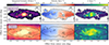 |
Fig. 2. HCN and CO(2–1) moment maps. Top row: HCN(1–0) moment maps: integrated intensity map (left), centroid velocity map (middle), and velocity dispersion (right). The beam size of 22″ is shown in the left corner of each panel. Bottom row: CO(2–1) moment maps, in the same order as for HCN(1–0). CO(2–1) is convolved to a beam size of 22″, and regrided to match the grid of HCN data. The black line shows the outline of the HCN emission from the top panels. We fix the colorscale for each moment map to highlight the differences and similarities in HCN and CO(2–1) emission. All maps are rotated so that the x- and y-axis show the angular distance from the NGC 253’s minor and major axis (see Table 1). |
The integrated intensity is computed as a sum of the emission along each line of sight (that is, we integrate along the velocity axis). We first create a CO(2–1) based mask. This mask is produced by selecting all voxels with a signal-to-noise ratio higher than four and then expanding it to include all contiguous voxels with signal-to-noise higher than 2. Next, we applied this mask to the HCN and CO(2–1) data cubes. The moment maps are derived from the masked data cubes using the python package SpectralCube (Ginsburg et al. 2019).
The HCN emission shows a clumpy structure and compact emission, prominent in the center of the galaxy and also concentrated along the ring and the bar. There are spots of bright HCN emission located at the contact points of the bar, dust lanes, and ring, which we also see in the ΣSFR (Figure B.1). These bright spots of HCN emission are expected to be found in the regions where the bar and ring intersect, as these are interfaces where gas orbits converge (Kenney 1994; Beuther et al. 2017). Moreover, we see CO(2–1) bright spots co-spatial with those seen in HCN.
The moment one map is the intensity-weighted mean velocity map. We show these in the middle column of Figure 2 for both HCN and CO(2–1). The velocity map is corrected for the systemic velocity (Table 1). The outskirts of the map (left and right side) show the highest velocity difference, that is, along the major axis (around −230 and +230 km/s on the eastern and western parts, respectively). The northeastern side of the galaxy is blue-shifted. HCN and CO(2–1) velocities look mainly consistent across the disk of NGC 253 (we discuss this in detail in Section 4). We expect their consistency from the assumption that HCN traces denser gas than the CO, thus probing denser molecular substructures traced by the CO emission. We note a few regions within which we observe discrepancy in centroid velocities of HCN and CO(2–1) and further discuss when considering spectral complexity along the line of sight in Section 4.
The second-moment map represents the velocity dispersion of the observed emission. The broadest line profiles are observed toward the center of this galaxy in both HCN and CO emission. Apart from the center, we also note other regions with relatively large velocity dispersion (∼50 km/s) in the HCN and CO(2–1) emission, such as the bar and partially the ring. CO(2–1) shows higher velocity dispersion than the HCN, and this difference becomes more notable at the outer parts of our map.
3. Line of sight HCN emission
3.1. Radial distribution of the line of sight HCN intensity
To investigate the HCN emission across NGC 253, we resample the HCN map on a hexagonal grid where adjacent pixels are half-beam spaced. We show the radial distribution of the HCN integrated intensity in Figure 3. We detect significant HCN emission up to ∼6.5 kpc. The high inclination of this galaxy causes large deprojected distances from the center along the minor axis (the minor axis effect). After inspection of the deprojected distances along the major axis, where we do not expect to encounter such an impact, we conclude that the farthest data point from the center of the map has a deprojected distance of 5.3 kpc, assuming an axisymmetric distribution. Consequently, data points at radii higher than 5.3 kpc should be taken cautiously when interpreting such radial trends. In addition, this effect will blur the observing trends. The uncertainty of the inclination (Table 1) affects the calculated radial distances by a factor of 0.4.
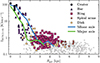 |
Fig. 3. HCN-integrated intensity as a function of the galactocentric radius. The colored, filled points represent pixels with a signal-to-noise ratio of three and above, whereas open points have a signal-to-noise ratio lower than three. |
Next, we extracted sight lines from each environment by applying the environmental mask (Querejeta et al. 2021) and color-code the points by the environment, following the color scheme used in Figure 1. The HCN intensity distribution in NGC 253 follows the CO(1–0) distribution described in Sorai et al. (2000) and Paglione et al. (2004), that is, the “twin-peaks” morphology, typical for barred galaxies (Kenney et al. 1992). The brightest HCN emission is located at the center of the galaxy, which is also seen in other galaxies: at kpc resolution in the EMPIRE (Jiménez-Donaire et al. 2019) and ALMOND (Neumann et al. 2023), in M 51 (Bigiel et al. 2016), in nearby galaxies at similar spatial scales (∼0.5 kpc, Gallagher et al. 2018b), and at higher spatial resolution in NGC 3627 (Bešlić et al. 2021). There is a steep decrease in HCN intensity by two orders of magnitude along the bar. Moreover, the HCN intensity varies by order of magnitude at distances of rgal > 2 kpc, coincident with the ring and spiral arms. With increasing distance from the center of NGC 253, we also note a decrease in the HCN emission, particularly in the inner 1–2 kpc region within the bar where HCN intensity decreases steadily by order of magnitude, similar to the barred galaxy NGC 3627 (Bešlić et al. 2021).
Ancillary observations of the CO(1–0) emission at similar spatial resolution (16″ ∼250 pc) across NGC 253 (Sorai et al. 2000; Paglione et al. 2004) show similar radial trends. Sorai et al. (2000) observed a secondary peak in CO(1–0) surface density around rgal = 2 kpc, located at the end of the bar. In our case, we observe a similar increase in the CO(2–1) emission at a distance between 3 and 4 kpc from the center of NGC 253, right outside the bar. In addition, we observe local enhancements in HCN in regions where the bar and the ring overlap and a decrease in HCN emission in the outermost parts of our map. By comparison, Sorai et al. (2000) found a decrease in CO(2–1) surface brightness by two orders of magnitude in the inner 1–2 kpc region of NGC 253, and the intensity after the second peak observed at 2 kpc is steadily decreasing. Moreover, the rotation curve of NGC 253 derived from the CO(1–0) emission (Koribalski et al. 1995; Sorai et al. 2000) flattens in the ring, which suggests that molecular gas at these positions starts losing its angular momentum and infalling toward the center (Sorai et al. 2000).
3.2. Line of sight HCN/CO(2–1) intensity ratio
The ratio of HCN to CO(1–0) is often used within the literature to constrain the dense gas fraction, fdense (Leroy et al. 2017b). Knowing the scaling between J = (1 − −0) and J = (2 − −1) intensity ratio (for instance, Sandstrom et al. 2013; Zschaechner et al. 2018; den Brok et al. 2021; Leroy et al. 2022), it is possible to use HCN/CO(2–1) for determining the fdense. In the case of NGC 253, we are particularly interested in seeing how this line ratio varies across the galaxy and search for any environmental dependence.
We calculated the HCN/CO(2–1) integrated intensity ratio from the hexagonally, half-beam-sized sampled grid data points at 22″. The uncertainty of the HCN/CO(2–1) ratio is computed from the uncertainties of their integrated intensities, using the standard error propagation technique (see for example, Bešlić et al. 2021; Eibensteiner et al. 2022). Figure 4 shows the HCN/CO(2–1) line intensity ratio as a function of a distance from the center of NGC 253. The radial distribution of HCN/CO(2–1) follows the trends seen in the HCN emission (Figure 3). It decreases toward larger galactocentric distances. The highest values (from 0.1 to 0.13) of this line ratio are found within the center of NGC 253. The transition from the central region to the disk is sharp, especially in the inner 2 kpc region of NGC 253 along the bar, where the HCN/CO(2–1) decreases by an order of magnitude. This finding is similar to the results reported in previous studies (Bigiel et al. 2016; Jiménez-Donaire et al. 2019; Gallagher et al. 2018b; Querejeta et al. 2019), whereas the weak radial variation of HCN/CO(2–1) intensity ratio across NCG 3627 is found in Bešlić et al. (2021). In the rest of the environments, particularly in the ring, spiral arms and the disk, the HCN/CO(2–1) intensity ratio does not vary significantly (values between 0.01 and 0.05). We note exceptionally high values of the HCN/CO(2–1) intensity ratio at distances larger than 6 kpc, which arises from the fact that at these distances, CO(2–1) emission appears to decrease more rapidly than the HCN.
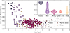 |
Fig. 4. Radial distribution of the HCN/CO(2–1) intensity ratio across NGC 253. Sight lines are color-coded based on the environment. We show points with a signal-to-noise ratio above three in intensity and the peak brightness temperature. A small panel in this figure shows the distribution of the HCN/CO(2–1) line intensity ratio per environment in NGC 253: the center, bar, ring, spiral arms, and disk. The mean line ratio measured in each environment is shown as a horizontal line. |
To quantify HCN/CO(2–1) in these environments, we show the distribution of this line ratio in each region as a violin plot in the upper right corner of Figure 4. In this panel, the length of each violin corresponds to the range of HCN/CO(2–1) intensity ratios. In contrast, the horizontal line indicates the mean measured in each environment. Points located in the center of NGC 253 have the highest mean of HCN/CO(2–1) of 0.1197 ± 0.0002, about 4 times higher than the median values found in the rest of the galaxy. The bar shows the widest distribution and possible bimodal behavior. The first group of sight lines has a high HCN/CO(2–1) ratio of 0.1 and above, close to those found in the center. The second group of points contains HCN/CO(2–1) values similar to those seen in the ring and the rest of the regions (from 0.01 to 0.08). Therefore, the bar represents an intermediate region that bridges the center and the rest of the environments found in NGC 253. The enhancement in the HCN/CO(2–1) ratio found has a few possible implications, which we discuss in more detail in Section 6.1.
The observed HCN/CO(2–1) line ratio shows agreement within the literature data for other galaxies. Similar to Gallagher et al. (2018b), Jiménez-Donaire et al. (2019), and Bešlić et al. (2021), this line ratio has the highest values in the inner ∼500 pc region of the galaxy, that is, the vast majority of the dense molecular gas relative to bulk molecular content is found within the center of a galaxy. Knudsen et al. (2007) found HCN/CO(1–0) ratio in the inner 1 kpc region to be 0.08. By applying the R21 line ratio of 0.8 (Zschaechner et al. 2018), we obtain higher values of HCN/CO(1–0). As opposed to HCN/CO(2–1) in the barred galaxy NGC 3627 (Bešlić et al. 2021), we see a stronger environmental dependence of HCN/CO(2–1) and a significant decrease toward higher galactocentric radii.
4. Decomposed HCN emission
To characterize the gas structure along each line of sight and its variation with the galactic environment, we study the spectra of the HCN emission in five different dynamical zones. We used a Semi-automated multi-COmponent Universal Spectral-line fitting Engine (SCOUSE; Henshaw et al. 2016, 2019) to decompose the observed emission into separate components along each line of sight. This program is developed to analyze spectral lines and extract information (such as centroid velocity, line width) from modeling the shape of a spectral line. Appendix C provides a detailed description of using SCOUSE. We show the number of HCN velocity components identified by SCOUSE on the left panel of Figure 5. Figure 5 shows examples of 4 spectra originating from different dynamical regions (center, bar, ring, and spiral arms –, each marked with a black rectangle on the left panel of Figure 5). In particular, lines of sight from the central region and the bar have multiple line profiles, whereas spectra toward the ring structure, spiral arms, and the disk are mainly narrow and single-peaked (the right panel in Figure 5). Similarly, Sorai et al. (2000) found compound velocity structures in CO(1–0), particularly within the bar. However, this is not due to the line broadening caused by galactic rotation within the beam. Instead, Sorai et al. (2000) proposed that strong non-circular motions cause two velocity components along the line of sight.
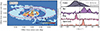 |
Fig. 5. HCN spectrum across NGC 253. Left: map of NGC 253 showing the number of velocity components in HCN emission across each pixel derived from SCOUSE. Right: example of HCN spectra from each environment shown in Figure 1 and from colored points on the left panel. The dashed black lines show each Gaussian velocity component derived from the SCOUSE spectra decomposition analysis (Henshaw et al. 2016, 2019). |
In Figure 6, we present our results from applying the SCOUSE analysis to HCN and CO(2–1) datasets. Each panel of the figure shows the distribution of fitting parameters describing a Gaussian line shape derived from SCOUSE, which include the number of components, peak temperature, centroid velocity, and velocity dispersion. Furthermore, these parameters are divided according to each environment.
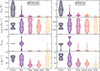 |
Fig. 6. Results from the SCOUSE decomposition. Here, we show Gaussian fit parameters: peak brightness temperature (first row), centroid velocity (second row), number of components (third row), and velocity dispersion (bottom row) derived from SCOUSE. The left column shows the results from decomposing the HCN emission, whereas the right column shows output parameters computed for the CO(2–1) emission. We show results for each environment. Distribution for HCN emission along the disk is represented as a circle since there was no converging fits. |
As shown in Figure 5, each environment contains different spectral features in HCN and CO(2–1). CO(2–1) profiles are generally brighter than HCN, and the spectra within the center, followed by those in the bar, have the highest temperature peaks. The distribution of Tpeak within the center has the largest dynamical range compared to the Tpeak determined in spectra from other environments.
The third row in Figure 6 summarizes what has been demonstrated in Figure 5. The highest number of velocity components is seen toward the bar and nuclear region. HCN spectra are predominantly double and triple-peaked in these regions, unlike HCN spectra in the ring, spiral arms, and disk. We find similar spectral complexity of the CO(2–1) emission. In addition, we identify several pixels whose CO(2–1) spectrum shows three velocity components in the bar and only a few pixels containing three HCN velocity components. Two scenarios could explain the lower frequency of multiple components observed in the HCN emission than in the CO(2–1) spectrum. The first explanation is that the HCN emission is generally fainter than CO(2–1). In this scenario, assuming that each CO(2–1) has its own HCN partner and the new CO(2–1) component along the same line of sight has a considerably lower signal-to-noise ratio than the previous one, it would explain why more HCN components were not detected. In the other case, since CO(2–1) and HCN trace overall different gas densities, it may occur that certain CO(2–1) clouds do not contain denser subregions possibly traced by HCN. The number of CO(2–1) velocity components toward each sight line within the ring and spiral arms is mostly one, except for a few lines of sight where we identify two CO(2–1) velocity features within the same pixel, possibly due to higher CO(2–1) sensitivity.
Next, we comment on the individual velocity dispersion of HCN and CO(2–1). Here, the environmental dependence becomes prominent as in Tpeak. Central sight lines show the broadest lines, followed by sight lines from the bar. The distribution of HCN and CO(2–1) velocity dispersion in the center has a bimodal behavior. The broadest is the σ distribution within the bar in HCN and CO(2–1)Ṫhe distribution of σ in HCN and CO(2–1) is compact in the rest of the environments. The highest median in σ is found within the center (55 km s−1 and 65 km s−1 for the HCN and CO(2–1)). Interestingly, within the bar, we find higher median values in HCN (40 km s−1) than in CO(2–1) emission (30 km s−1). In the ring and spiral arms, the median σ in CO(2–1) is higher than in HCN. The lines of sight across the disk show broad HCN and CO(2–1) components. These lines of sight are close to the center of NGC 253 (see Figure 3).
4.1. Decomposed HCN/CO(2–1) line intensity ratio
This section investigates the HCN/CO(2–1) intensity ratio derived from SCOUSE and compares it with our previous findings described in Section 3. To directly compare HCN and CO(2–1) intensities from each component derived from SCOUSE, it is necessary to match the detected velocity components in HCN with those found in the CO(2–1) emission. As seen on the top left panel of Figure 6, the number of Gaussian components differs from region to region and between HCN and CO(2–1). This could result from the CO(2–1) tracing more lower density gas at shifted velocity to which the HCN is not sensitive.
The first step in associating velocity components is to look at the centroid velocities determined for each component within each pixel in HCN and CO(2–1), particularly the difference in υcentroid, HCN and υcentroid, CO(2 − 1). When the HCN velocity component is associated with the CO(2–1), their centroid velocities should be similar. Therefore, we consider that the HCN line is associated with the CO(2–1) if:
 (5)
(5)
We define the σthresh as follows:
 (6)
(6)
and calculate this value for each pixel where we decompose the emission. Equations (5) and (6) represent the overlap of the clouds. Such a criterion assures us that clouds with higher line widths have a less strict association criterion. After applying this threshold, we match 100% of HCN emission lines to those in CO(2–1) in the center, ring, and spiral arms. We matched 78% of HCN emission to the CO(2–1) components within the bar. Around 60% of the CO(2–1) flux entering this analysis (see Section 2.3) is associated with the HCN emission. In exceptional cases, when two components have similar centroid velocities, we take the one with higher amplitude, that is, the Tpeak.
Similarly, as in Figure 4, in Figure 7 we show the component-by-component HCN/CO(2–1) intensity ratio as a function of distance from the center of NGC 253 (left panel) and the distribution of this line ratio within each environment (right panel). The radial distribution of the component-by-component HCN/CO(2–1) is similar to that of the line of sight HCN/CO(2–1) (Figure 4). We also observe here the center showing the highest HCN/CO(2–1) ratio, followed by the bar. Similarly, as in Figure 4, we observe a steady decrease in HCN/CO(2–1) at distances of 1 − 2 kpc. By comparing the distributions of HCN/CO(2–1) computed from SCOUSE with those presented in Section 3.2 (dashed violin shapes on the right panel in Figure 7), we see the biggest difference between these two approaches in the center. Although the means of these two distributions are similar, their shape is different, that is, the decomposed HCN/CO(2–1) distribution is significantly elongated than the line of sight distribution. The distributions of data points using both approaches within the bar are similar; they both show signs of bimodal behavior, but their mean values differ. The mean of the HCN/CO(2–1) from SCOUSE is comparable to the mean values calculated from the line of sight line ratio. Moreover, distributions of HCN/CO(2–1) of spiral arms and disk derived from SCOUSE are different from the line of sight HCN/CO(2–1), mainly because of a generally lower signal-to-noise ratio of the HCN emission in these environments, which resulted in a lower number of successfully decomposed lines of sight.
4.2. HCN velocity dispersion
Molecular gas flows impact the dynamical state of the gas (Meidt et al. 2018) and lead to collisions and gas crowding (Beuther et al. 2017), thus possibly suppressing or enhancing star formation. This directly impacts the star formation efficiency, which is in line with turbulent models of star formation (Federrath & Klessen 2013). On the one hand, whether tied to galactic gas flows or star formation feedback, super-virial gas motions can reduce star formation efficiencies (Padoan & Nordlund 2011; Meidt et al. 2018). On the other hand, large velocity dispersions may signify elevated Mach numbers and a preferential build-up of dense gas (Krumholz & McKee 2005; Federrath & Klessen 2012; Gensior et al. 2020).
The environments studied here represent a diversity of gas flows and conditions: strong shear in the center, elliptical streaming motions and strong radial inflows in the bar, a pile-up of gas in the ring, and strong spiral streaming motions. Here, we investigate the sensitivity of the gas velocity dispersion to these environments. We also explore how the velocity dispersion of dense gas compares to that of molecular gas. Dense gas arising from the small scales might be expected to be less sensitive to the flows present at or just beyond the cloud envelope, while its presence may reveal signatures of the critical role that colliding flows and shear have on the gas structure.
We compare the observed velocity dispersion in NGC 253 for HCN and CO(2–1) emission in Figure 8. The solid black line represents the one-to-one ratio in HCN and CO(2–1) velocity dispersion. The HCN emission lines are narrower than the CO lines, as the data points typically lie below the diagonal line. This trend is particularly pronounced in the center and the bar, whereas data points are scattered around the solid black line at velocity dispersions below 50 km s−1. Central sight lines populate the higher-values region, whereas sight lines from the spiral arms (orange points) and the ring (pink points) have low values. Interestingly, bar sight lines are distributed over the full range of the observed values along both axes.
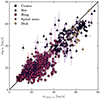 |
Fig. 8. Component-by-component comparison between the HCN (y-axis) and CO(2–1) (x-axis) velocity dispersion derived from spectral decomposition using SCOUSE. We color-coded each point by the environment. The diagonal, solid black line shows a 1:1 ratio between the x- and y-axis. |
The general positive correlation in HCN and CO(2–1) velocity dispersion in NGC 253 agrees with previous velocity dispersion measurements in M 51 (Querejeta et al. 2019), and across NGC 3627 (Bešlić et al. 2021). Our result confirms expectations that higher-density gas (traced by the HCN in our case) has smaller turbulent velocity dispersion than lower-density gas (traced by the CO(2–1)). This finding also agrees with the models that observed the building up of higher-density gas in the stagnation regions of convergent flows from the larger-scale turbulence. Consequently, the average velocity dispersion of the gas at these stagnation points will be smaller.
In Figure 9, we show decomposed HCN/CO(2–1) intensity ratio derived from SCOUSE as a function of the CO(2–1) velocity dispersion. Our data points populate two different parts of this figure. In particular, we note at σCO(2 − −1) of > 45 km s−1 higher HCN/CO(2–1) values, which is a consequence of the environment, as these data points are located in the bar and the center. In the case of lower velocity dispersions, the 16% and 84% of observed HCN/CO(2–1) lie in the range from 0.02 to 0.04
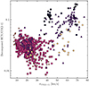 |
Fig. 9. Decomposed HCN/CO(2–1) intensity (y-axis) and the CO(2–1) velocity dispersion (x-axis). We color-coded each point by the environment, similar to in Figure 8. |
5. Dense molecular gas and star formation
5.1. Environmental dependence of the star formation efficiency of the dense gas
Previous extragalactic studies have shown different behavior of SFEdense across the disk of a galaxy. For example, regions with high stellar surface density and thus interstellar pressure, such as centers of galaxies, typically have relatively lower SFEdense, that is, the ability of dense gas to form stars is significantly reduced (for example, Longmore et al. 2013; Kruijssen et al. 2014; Usero et al. 2015; Bigiel et al. 2016; Barnes et al. 2017; Jiménez-Donaire et al. 2019; Bešlić et al. 2021; Eibensteiner et al. 2022). In the following, we investigate properties of star formation efficiency of dense gas SFEdense (usually traced by the LIR/Mdense) across NGC 253.
In Figure 10, we show the TIR/HCN luminosity (TIR/Mdense on the right y-axis) ratio as a function of the molecular gas surface density. Dashed vertical lines in both panels show the gas surface density thresholds presented in Bigiel et al. (2008). The left vertical line at ∼10 M⊙ pc−2 indicates the surface density above which the molecular gas dominates over the atomic phase (Bigiel et al. 2008), whereas the right vertical line shows the surface density threshold of ∼200 M⊙ pc−2, after which we enter the regime where dense molecular gas emission linearly scales with the star formation (Gao & Solomon 2004; Bigiel et al. 2008). The blue-shaded region corresponds to binned trends and their respective range of 16th and 84th percentiles. The horizontal shaded region shows a range of 400 − 500 L⊙/M⊙.
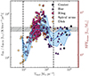 |
Fig. 10. SFR/HCN luminosity ratio as a proxy for the star formation efficiency of dense molecular gas as a function of Σmol. Points are color-coded according to their environments. Vertical dashed lines show the surface density thresholds of ∼10 M⊙ pc−2 and ∼200 M⊙ pc−2, previously defined in Bigiel et al. (2008). The horizontal shaded region shows a range of 400 − 500 L⊙/M⊙. |
Our HCN measurements are located in moderate density regimes (part of the bar, ring, spiral arms, and disk) and at high surface densities (lines of sight from the center and bar). That said, we do not have information about the HCN emission for molecular gas surface densities lower than a few M⊙ pc−2, where the atomic gas dominates the total gas surface densities (Bigiel et al. 2008). The lowest values of SFEdense are measured in the disk of NGC 253. At the intermediate surface densities (9–200 M⊙ pc−2), SFEdense rises with the cloud-scale molecular surface density up to ∼100 M⊙ pc−2, after which it starts decreasing. The mean SFEdense increases up to ∼500 L⊙/M⊙ in the intermediate density regime, while the high surface density part shows nearly constant SFEdense of ∼400 L⊙/M⊙. The lowest SFEdense in this regime have lines of sight at the bar.
The center of NGC 253 is characterized by strong tidal forces and generally high pressure, typical also for other galaxies (see Gallagher et al. 2018a). Therefore, tidal forces may impact the fraction of gas that is self-gravitating, which can lead to a reduction in the observed SFEdense when, at the same time, some part of the HCN-emitting gas is prevented from being in a state to collapse and form stars. Therefore, we suggest that the elevated average cloud density characteristic of the high-pressure central environment (Gallagher et al. 2018a) implies that a greater portion of the cloud emits HCN in the central regions of NGC 253.
The observed behavior of SFEdense presented in Figure 10 may result in the non-constant conversion factor XHCN. When XHCN varies, the relation between HCN luminosity and dense gas mass becomes non-linear, and consequently, the SFEdense will have intrinsic scatter. At the spatial scales probed in this work (300 pc), the temporal and environmental effects impact observed SFEdense, which are averaged out at larger scales.
In addition, it is important to consider the caveats of using the HCN emission as a proxy of dense gas, which has become especially important in regions with high mean gas density. As seen in Figure 10, SFEdense reaches a regime of 400 − 500 L⊙/M⊙ at which SFEdense becomes constant, also found in previous studies (Shirley & Evans 2003; Scoville & Wilson 2004; Thompson et al. 2005; Wu et al. 2010). In these high-density regimes, the HCN(1–0) emission does not necessarily probe pure star-forming gas, as, for example, in other regions, where mean gas densities are comparable or lower than the critical density of HCN(1–0) (Leroy et al. 2017a; Bešlić et al. 2021). Alternatively, higher J transitions of HCN can better probe dense gas mass relative to the average gas density in these regions. Therefore, excited HCN emission could be used to derive the XHCN factor at higher densities and constrain the dense gas mass, which is beyond the scope of this work.
5.2. Star formation efficiency and velocity dispersion
In this section, we investigate how the IR/HCN luminosity (and LIR/Mdense) ratio varies with velocity dispersion and environment in NGC 253. We show the SFEdense as a function of the HCN velocity dispersion inferred from SCOUSE decomposition (Section 4) in Figure 11. Similarly, as in Figure 8, data points populate two distinct parts of Figure 11. The first group of data points is located in the upper left part of the figure, showing HCN velocity dispersions lower than 40 km/s, whereas the second group shows σHCN> 40 km/s and lies at the bottom right part of the figure.
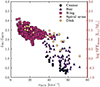 |
Fig. 11. Ability of dense gas to form stars, traced by the IR/HCN luminosity ratio, as a function of the HCN velocity dispersion measured from spectral decomposition analysis. We color-coded each point by the environment. |
The first group of data points consists of lines of sight from the ring and spiral arms, whereas the central lines of sight are in the second group. Lines of sight from the bar and the disk are found in both groups. The IR/HCN luminosity ratio decreases with increasing HCN velocity dispersion. This decrease is significantly steeper for data points with higher velocity dispersions. It is worth pointing out that the systemic rotation velocity is not necessarily resolved at our scales, which causes line broadening at the center. In addition, the observed anticorrelation between IR/HCN and σHCN comes from the correlation between CO and HCN intensities and their respective line widths. We note that, at the scales of our observations, the systemic rotation velocity is not fully resolved, which also broadens observed lines.
Nevertheless, broader molecular lines imply lower efficiency of such gas at star formation, and our results indicate that gas turbulence could be suppressing star formation (Padoan & Nordlund 2011; Meidt et al. 2018). Similar results are found in M 51 and NGC 3627 (Querejeta et al. 2019; Bešlić et al. 2021): central sight lines show broader emission lines, but the ability of such gas for star formation is reduced. Murphy et al. (2015) compared SFR/HCO+ with HCO+ line widths in the nuclear region and bar ends in NGC 3627 and concludes that the velocity dispersion of molecular is an important factor in setting star formation.
6. Discussion
6.1. Enhancement of the HCN/CO(2–1) ratio in the inner 2 kpc of NGC 253
In the following, we briefly discuss our results presented in Sections 3.1 and 3.2. As seen in Figure 3, the HCN integrated intensity generally decreases toward the higher galactocentric radii. The steepest change in the HCN intensity occurs in the inner 2 kpc region of NGC 253. Such behavior has been observed in previous studies probing similar or even smaller spatial scales (Bešlić et al. 2021; Neumann et al. 2023). Similarly, by looking at the radial trend of HCN/CO(2–1) intensity ratio (Figure 4), we observe change by a factor of ∼7 in the inner 2 kpc, at the location of a bar in NGC 253. The reason for such a steep decrease of the HCN, but also the CO(2–1) intensities could be due to the bad influence. However, we speculate that other mechanisms impact this enhanced HCN/CO(2–1) intensity ratio in the case of NGC 253. The starburst in this galaxy drives the outflow seen in various gas phases: in ionized gas (Hα and X-ray (Strickland et al. 2000, 2002; Westmoquette et al. 2011; Lopez et al. 2023), neutral gas (Heckman et al. 2000), warm H2 (Veilleux et al. 2009), OH both in emission and absorption (Turner & Ho 1985; Sturm et al. 2011). Moreover, this outflow contains a significant amount of dust (HST observations, Watson et al. 1996), molecular gas, based on ALMA CO(1–0) observations (Bolatto et al. 2013; Krieger et al. 2020), and dense molecular gas traced by HCN emission (Walter et al. 2017; Krieger et al. 2017).
The enhanced HCN/CO(2–1) in the bar toward the center of NGC 253 and the bimodal distribution for the bar sight lines in HCN/CO(2–1) have a few possible interpretations. On the one hand, we might witness a molecular gas flow, and there is a chance that enhanced HCN/CO(2–1) points in the bar originate from the molecular wind, as shown in Walter et al. (2017). On the other hand, beam-smearing effects caused by a high galaxy inclination are not negligible. Therefore, we may detect the emission from the center within the bar. Moreover, Paglione et al. (2004) found high gas densities traced by CO(1–0) emission near the inner Lindblad radius (∼300 pc, Iodice et al. 2014) and along the bar’s minor axis. We investigate these sight lines to explore further and explain the enhancement in HCN/CO(2–1).
The bar’s data points that form the upper locus of HCN/CO(2–1) (right panel of Figure 4) have values above 0.1. After inspecting the data points that cause the upper locus in the HCN/CO(2–1), we find that these points lie along the minor axis in NGC 253, that is, where we expect to see the outflow. It is worth noting that the spatial scales probed by our data are not sufficient to resolve the outflow. Nevertheless, it is still possible to see the signs of the outflow within the spectra. Walter et al. (2017) observed the wind in NGC 253 in CO(1–0) emission and found a separate velocity component at intermediate (−4″ to −10″) offsets from the major axis. Therefore, we plot the HCN spectrum, including the decomposed emission derived from SCOUSE (Section 4) toward the sight lines with enhanced HCN/CO(2–1) found along the minor axis, toward the direction of the brightest, southwestern (SW) streamer of the outflow (negative offsets from the minor axis). We show these in Figure 12. Each spectrum is colored by the HCN/CO(2–1) line intensity ratio.
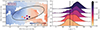 |
Fig. 12. HCN spectrum taken along the minor axis. Left: bar sight lines in NGC 253. We label major and minor axes. Colored points are sight lines showing enhanced HCN/CO(2–1) emission in the direction of the SW streamer (Walter et al. 2017) and that contribute to the bimodality seen in Figure 4. Colors correspond to their HCN/CO(2–1) intensity ratio shown in the colorbar. Right: HCN spectra toward the data points located along the minor axis in NGC 253 shown on the left. Each spectrum is colored by the HCN/CO(2–1) ratio shown on the colorbar. All these data points are located along the SW streamer (Walter et al. 2017). The black dashed line shows NGC 253 systemic velocity of 243 km s−1 (see Table 1). The black solid line represents the υlsr = 200 km s−1 velocity at which Walter et al. (2017) observed the outflowing component in CO(1–0) emission. |
Across all these points, we observe that the HCN emission consists of two components, the dominant one (dashed line) centered at velocities higher than 243 km s−1, and a second one (solid line) centered at velocities lower than −43 km s−1, consisted with the value for the outflow, υ = −43 km s−1 (Walter et al. 2017). We show this velocity as a solid black line in Figure 12, and systemic NGC 253 velocity as a black dashed line.
Walter et al. (2017) calculated HCN/CO(1–0) line intensity ratio in the outflow and the disk of NGC 253. This study found that the HCN/CO(1–0) is ∼0.1 in the outflow and three times lower value in the disk (1/30). We estimate the HCN/CO(1–0) ratio from our measurements. We use a mean R21 ratio of 0.8 measured in NGC 253 (Zschaechner et al. 2018). After applying the R21 ratio, sight lines with enhanced HCN/CO(2–1) line intensity ratio (from 0.1 to 0.12) correspond to values within the 0.080 to 0.096 range in HCN/CO(1–0). Therefore, the molecular outflow could explain the enhanced HCN/CO(2–1) intensity ratio found along the minor axis.
6.2. Molecular gas kinematics
The inner 500 pc region of NGC 253, also called the central molecular zone (CMZ), is characterized by a strong dust continuum emission (Leroy et al. 2018). The giant molecular clouds found in the CMZ of NGC 253 (Leroy et al. 2015) are more massive and have higher velocity dispersion than the GMCs in the Milky Way (Krieger et al. 2020). These clouds contain young massive clusters, bright in continuum and line emission (Leroy et al. 2015, 2018), with detected large-scale outflow in dense molecular (Levy et al. 2021) and ionized gas (Mills et al. 2021).
Meier et al. (2015) provided a schematic representation of the central region in NGC 253, demonstrating its interesting and complex structure. These authors found that the nuclear disk has an inner and outer region (∼170 pc and ∼400 pc). The inner nuclear disk contains high-density molecular gas and intense star formation. In contrast, the outer nuclear disk is considered the region where gas flows inward along the large-scale bar (Sorai et al. 2000; Paglione et al. 2004; Meier et al. 2015).
We show the position–velocity diagram in Figure 13 of the centroid velocities of HCN emission from the SCOUSE as a function of the offset from the galaxy’s minor axis. Each point is color-coded by the HCN/CO(2–1) integrated intensity and the environment. The HCN/CO(2–1) is derived from the integrated intensities calculated from SCOUSE (see Section 7). Bar sight lines tend to form a “parallelogram”-shaped feature in the pv plane, previously seen in CO(1–0) (Sorai et al. 2000) and CS(2–1) emission (Peng et al. 1996), consistent with gas flowing in a bar potential (Binney et al. 1991; Athanassoula 1992; Peng et al. 1996; Sormani et al. 2015). We note that there are more data points on the leading side of the bar (bottom left part of Figure 13), which is indicative of molecular gas concentrations caused by a non-axisymmetric bar potential (Kuno et al. 2000). The velocity gradient is steepest in the bar and center and shallow in the ring and spiral arms. As the molecular gas travels from the outer disk, it starts losing angular momentum at galactocentric radii lower than the corotation radius ∼3 − 4 kpc (Iodice et al. 2014), and is accreted onto the ring. The rotation curve within the ring is almost flat, causing the crowding of molecular gas, which is likely supported by the observed narrow, single-peaked HCN spectral features.
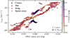 |
Fig. 13. Position–velocity diagram (pυ) of the HCN emission in NGC 253. The y-axis shows the centroid velocities from the spectral decomposition, and the x-axis shows the angular distances from the minor axis of NGC 253. We color-coded points by their HCN/CO(2–1) ratio derived from SCOUSE, and the size of each point corresponds to the HCN velocity dispersion. |
6.3. Star formation efficiency
In Figure 14, we summarize previous HCN surveys and studies, including recent ones (for example, results from the ALMOND survey Neumann et al. 2023). We show the relation of HCN luminosity and dense gas mass relation to star formation on the top left panel of Figure 14, and to the TIR/HCN luminosity ratio and LIR/Mdense (top right panel, see also Jiménez-Donaire et al. 2019).
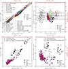 |
Fig. 14. Summary of previous dense gas studies. Top left: literature overview of the infrared luminosity (a proxy for the star formation rate) as a function of the HCN luminosity (a proxy for dense molecular gas), that is, the Gao and Solomon relation (Gao & Solomon 2004). We show measurements of whole galaxies and their centers at a few kpcs (see the legend in the upper and the lower-left of the panel), Milky Way clouds (a few pc scales - see legend on the bottom right), including measurements across NGC 253 (this work - see the legend on the right central part) (Jiménez-Donaire et al. 2019). The dark red line shows a 500 M⊙/L⊙ which corresponds to a upper limit reported in Scoville & Wilson (2004) and Thompson et al. (2005). Top right: same as in the left panel, but we are now showing SFEdense, traced by the IR/HCN luminosity ratio on the y axis. In both panels, the black solid line shows the mean IR/HCN luminosity ratio measured by the EMPIRE survey (Jiménez-Donaire et al. 2019). Black dashed lines show the 1σ RMS scatter of ±0.37 dex in units of L⊙/(K km s−1 pc2). Bottom row: zoomed-in view of the field from Figure 14, where we show NGC 253 sight lines, points from the nearby starburst galaxy M 82 (Kepley et al. 2014), the merging system of the Antennae galaxies (Bigiel et al. 2015), and a sample of LIRGs and ULIRGs (García-Burillo et al. 2012). Axes are the same as of the panels at the top row. Data points from Kepley et al. (2014) have different shades of gray that corresponds to the distance to the center of M 82, where the darkest points have the smallest galactocentric distances. |
We observe an approximately linear correlation between IR and HCN luminosities. As seen from the top panels of Figure 14, the literature overview shows this correlation spanning more than ten orders of magnitude, covering a wide range of physical scales, from dense clumps and cores (a few parsecs; Wu et al. 2010; Stephens et al. 2016) within the Milky Way, to GMCs in local and nearby galaxies (Chin et al. 1997, 1998; Braine et al. 2017; Brouillet et al. 2005; Buchbender et al. 2013; Chen et al. 2017; Querejeta et al. 2019), measurements of resolved galaxy disks (a few kpcs Kepley et al. 2014; Usero et al. 2015; Bigiel et al. 2016; Chen et al. 2015; Gallagher et al. 2018b; Tan et al. 2018; Jiménez-Donaire et al. 2019; Jiang et al. 2020) to whole galaxies and their centers (Gao & Solomon 2004; Gao et al. 2007; Krips et al. 2008; Graciá-Carpio et al. 2008; Juneau et al. 2009; García-Burillo et al. 2012; Crocker et al. 2012; Privon et al. 2015; Puschnig et al. 2020). By observing this trend, a direct conclusion is that denser molecular gas implies a higher star formation rate.
Therefore, we investigate how our results fit the relationship between star formation and dense molecular gas within the literature. We also include measurements from this work on NGC 253, colored by different regions in this galaxy in Figure 14.
Our measurements span approximately three orders of magnitude in IR luminosity and dense gas mass. Lines of sight from NGC 253 fall into the same region of the SFR-HCN plane as measurements of whole galaxies and parts of galaxies. The center of NGC 253 contains the largest amount of dense gas and shows the highest star formation activity, unlike the rest of the NGC 253’s environments. By contrast, in the top right panel, we note that regions with the brightest HCN emission in NGC 253 have the lowest SFEdense. This is in agreement with previous studies. For instance, the CMZ, the densest and most active region in our Galaxy, shows an order of magnitude lower SFR than those predicted from measurements of dense molecular gas (Longmore et al. 2013; Henshaw et al. 2023). In extragalactic work, Jiménez-Donaire et al. (2019) and Neumann et al. (2023) observed reduced SFEdense toward centers of nearby galaxies, despite containing most of the Mdense and the highest fdense. Querejeta et al. (2019) have shown that gas in spiral arms has large SFEdense in M 51. Similarly, bar ends in NGC 3627 show higher SFEdense than the center of this galaxy (Bešlić et al. 2021).
To first order, this relation seen in top panels of Figure 14 suggests a universal density threshold above which gas starts to form stars (Lada et al. 2012). However, the systematic scatter in the right panel in Figure 14 implies that not all dense gas is equally efficient at star formation, that is, SFEdense is environmentally dependent. On the one hand, this could imply a physical change in LIR/Mdense, possibly driven by dynamical effects such as turbulence and stellar feedback (Padoan & Nordlund 2011; Federrath & Klessen 2012) that become important at GMC scales (Gallagher et al. 2018b; Querejeta et al. 2019; Sánchez-García et al. 2022; Neumann et al. 2023). In addition, as previously discussed in Section 5.1, a systematic variation in XHCN can cause the observed scatter. On the other hand, even in the case of a constant conversion factor between the HCN luminosity and dense gas mass, it is possible that HCN might not be a reliable linear tracer of Mdense, resulting in not all HCN-tracing gas taking part in star formation.
In the bottom panels of Figure 14, we compare our results with other HCN observations across other starburst systems. We show measurements from Kepley et al. 2014 across the nearby starburst galaxy M 82 at slightly smaller physical scales (200 pc) than our work the sample of ULIRGs from García-Burillo et al. (2012), and sight lines from the galaxy merger, Antennae at 700 pc (Bigiel et al. 2015). LIRGs and ULIRGs show elevated IR and HCN luminosity, two orders of magnitude higher than starburst systems. M 82 sight lines appear to have higher IR luminosity than NGC 253. The center of M 82 exhibits the brightest HCN emission (gray diamonds in the bottom row of Figure 14 Kepley et al. 2014), although it is fainter than the HCN emission toward the center of NGC 253. M 82 and NGC 253 are both typical starburst galaxies. However, these galaxies go through a different evolutionary phase (Rieke et al. 1988) and have different magnitudes of starburst. NGC 253 is in the earlier starburst stage than M 82 (∼10 M⊙ yr−1 Telesco et al. 1991). In addition, M 82 is a gas-rich starburst triggered by a major interaction with M 81. Therefore, we expect a higher fraction of HCN-tracing gas across NGC 253.
Looking at the top right panel in Figure 14, we note scatter in the IR/HCN ratio of ∼3 dex for all sources. Overall, among each source presented in this figure, we observe that lines of sight with the highest HCN luminosities have the lowest star formation efficiencies, except M 82, where this trend is unclear. LIRGS and ULIRGS (García-Burillo et al. 2012), together with measurements of M 82 (Kepley et al. 2014), have the highest star formation efficiencies.
The results discussed in this section are consistent with the known role of the HCN-tracing gas in star formation, that is, that higher HCN luminosity implies higher star formation rate, but that the scatter in IR/HCN as a function of HCN luminosity is not negligible. We observe environmental dependence on the observed IR/HCN with dense gas mass, as confirmed in several previous studies (Jiménez-Donaire et al. 2019). However, The still observed scatter remains to be explained by future more sensitive, high-resolution observations across nearby galaxies that can probe the physical properties of individual molecular clouds.
7. Summary
We present new ALMA ACA+TP observations of HCN emission at 300 pc scales across the closest southern starburst galaxy NGC 253. These observations cover a large portion of the NGC 253 disk that contains 95% of detected CO(2–1) emission obtained by ALMA ACA, and 85% of the star formation activity measured from ancillary infrared data at 70, 160, and 250 μm obtained by the Herschel Space Telescope (Pilbratt et al. 2010). Our work investigates the HCN line intensity distribution, its relation to the CO(2–1) emission, gas kinematics traced by this molecular line, the ability of gas to form stars, and the environmental dependence of these properties. Here we summarize our results:
-
We used two independent methods to derive the integrated intensity of HCN emission. The first approach is based on calculating the zeroth moment map and extracting the information of HCN emission from it. In contrast, the second one uses information derived from the spectral decomposition of the observed emission along each line of sight. By performing spectral decomposition, we gain insight into the velocity components that contribute to the observed line emission at each point.
-
Our results derived from both methods are in good agreement. We find environmental differences in the observed HCN emission across NGC 253, particularly in regions closer to the center and regions in the disk. The HCN emission is strongly enhanced toward the center of NGC 253, and its intensity decreases by two orders of magnitude along the bar. HCN intensity weakly varies along the ring, spiral arm, and disk.
-
In addition, the HCN spectrum shows complexity and environmental dependence. In the inner 2 kpc region, we observe multiple velocity structures in the HCN and CO(2–1) spectra. Using spectral decomposition, we find up to three separate velocity structures in the central and bar sight lines, indicating that our observations probe multiple gas flows. Moreover, HCN and CO(2–1) spectral lines within the ring structure and spiral arms are mainly single-peaked and significantly narrower than the spectra from the inner regions. Our results support the idea that the molecular gas sits in the ring, after which it is inflowing toward the nuclear region along the bar.
-
We investigate the HCN/CO(2–1) line intensity ratio and its environmental distribution in NGC 253. We find that the HCN/CO(2–1) distribution within the bar shows bimodal behavior, which is a consequence of beam-smearing effects and a possible indication of the molecular outflow found in Walter et al. (2017). A nearly constant HCN/CO(2–1) intensity ratio within the ring, in line with the flattened rotational curve of CO at this region, suggests that molecular gas traced by HCN emission gets piled up in that region.
-
The majority of the decomposed HCN emission has an associated CO(2–1) component. All lines of sight in the ring, spiral arms, and disk have HCN emission associated with the CO(2–1). In contrast, in inner regions, the percentage of associated components is somewhat lower, which could be due to opacity broadening, a lower signal-to-noise ratio in HCN than CO(2–1) emission, but also because some of the CO(2–1) is diffuse and does not contain HCN. Together with spectral complexity, we find the environment to be the driver of the measured HCN velocity dispersion and broader HCN lines in regions with different dynamical characteristics.
-
Wider CO(2–1) profiles contain wider HCN emission lines, and CO(2–1) emission lines are broader than HCN lines, suggesting that HCN-tracing gas arises from smaller spatial structures. This result aligns with turbulence theory, which predicts that high-density gas is mostly seen at the stagnation regions of larger-scale convergent flows.
-
We investigate the ability of the gas to form stars as a function of the relative amount of HCN-traced molecular gas to bulk molecular gas. Lines of sight with the highest HCN/CO(2–1) ratio appear the least efficient at star formation (the lowest IR/HCN). This result suggests that the processes that regulate star formation vary with the environment.
Our work illustrates the importance of mapping the spatially resolved emission of the molecular gas tracing star-forming content on the example of NGC 253. In this work, we also analyze the spectrum of these lines along individual lines of sight. We highlight the necessity of extending our understanding of dense gas properties across starburst systems such as NGC 253 since they provide additional constraints on the dense gas properties in the vicinity of extreme physical conditions, particularly in its center.
Data availability
The reduced HCN map is available at the CDS via anonymous ftp to cdsarc.cds.unistra.fr (130.79.128.5) or via https://cdsarc.cds.unistra.fr/viz-bin/cat/J/A+A/689/A122
Acknowledgments
We thank the anonymous referee for their insightful comments that improved this manuscript. The author wants to thank Maryvonne Gerin and Jerome Pety for their insightful discussion that contributed to the quality of this work. This paper makes use of the following ALMA data: ADS/JAO.ALMA#2019.2.00236.S and ADS/JAO.ALMA#2018.1.01321.S. ALMA is a partnership of ESO (representing its member states), NSF (USA) and NINS (Japan), together with NRC (Canada), MOST and ASIAA (Taiwan), and KASI (Republic of Korea), in cooperation with the Republic of Chile. The Joint ALMA Observatory is operated by ESO, AUI/NRAO and NAOJ. In addition, publications from NA authors must include the standard NRAO acknowledgement: The National Radio Astronomy Observatory is a facility of the National Science Foundation operated under cooperative agreement by Associated Universities, Inc. IB, ATB, and FB would like to acknowledge the funding provided from the European Union’s Horizon 2020 research and innovation programme (grant agreement No 726384/Empire). HAP acknowledges support by the National Science and Technology Council of Taiwan under grant 110-2112-M-032-020-MY3. KG is supported by the Australian Research Council through the Discovery Early Career Researcher Award (DECRA) Fellowship DE220100766 funded by the Australian Government. KG is supported by the Australian Research Council Centre of Excellence for All Sky Astrophysics in 3 Dimensions (ASTRO 3D), through project number CE170100013. MC gratefully acknowledges funding from the DFG through an Emmy Noether Research Group (grant number CH2137/1-1). COOL Research DAO is a Decentralized Autonomous Organization supporting research in astrophysics aimed at uncovering our cosmic origins. JMDK gratefully acknowledges funding from the European Research Council (ERC) under the European Union’s Horizon 2020 research and innovation programme via the ERC Starting Grant MUSTANG (grant agreement number 714907). RSK acknowledges support from DFG via the collaborative research center “The Milky Way System” (SFB 881; project ID 138713538; sub-projects B1, B2 and B8), from the Heidelberg cluster of excellence EXC 2181“STRUCTURES” (project ID 390900948), funded by the German excellence strategy, from ERC via the synergy grant “ECOGAL” (grant 855130), and from the German Ministry for Economic Affairs and Climate Action for funding in project “MAINN” (funding ID 50OO2206).
References
- Aladro, R., Martín-Pintado, J., Martín, S., Mauersberger, R., & Bayet, E. 2011, A&A, 525, A89 [NASA ADS] [CrossRef] [EDP Sciences] [Google Scholar]
- Anand, G. S., Lee, J. C., Van Dyk, S. D., et al. 2021, MNRAS, 501, 3621 [Google Scholar]
- Aniano, G., Draine, B. T., Gordon, K. D., & Sandstrom, K. 2011, PASP, 123, 1218 [Google Scholar]
- Arnaboldi, M., Capaccioli, M., Cappellaro, E., Held, E. V., & Koribalski, B. 1995, AJ, 110, 199 [CrossRef] [Google Scholar]
- Athanassoula, E. 1992, MNRAS, 259, 345 [Google Scholar]
- Barnes, A. T., Longmore, S. N., Battersby, C., et al. 2017, MNRAS, 469, 2263 [Google Scholar]
- Beuther, H., Meidt, S., Schinnerer, E., Paladino, R., & Leroy, A. 2017, A&A, 597, A85 [NASA ADS] [CrossRef] [EDP Sciences] [Google Scholar]
- Bešlić, I., Barnes, A. T., Bigiel, F., et al. 2021, MNRAS, 506, 963 [CrossRef] [Google Scholar]
- Bigiel, F., Leroy, A., Walter, F., et al. 2008, AJ, 136, 2846 [NASA ADS] [CrossRef] [Google Scholar]
- Bigiel, F., Leroy, A. K., Blitz, L., et al. 2015, ApJ, 815, 103 [NASA ADS] [CrossRef] [Google Scholar]
- Bigiel, F., Leroy, A. K., Jiménez-Donaire, M. J., et al. 2016, ApJ, 822, L26 [NASA ADS] [CrossRef] [Google Scholar]
- Binney, J., Gerhard, O. E., Stark, A. A., Bally, J., & Uchida, K. I. 1991, MNRAS, 252, 210 [Google Scholar]
- Bisbas, T. G., Papadopoulos, P. P., & Viti, S. 2015, ApJ, 803, 37 [NASA ADS] [CrossRef] [Google Scholar]
- Bolatto, A. D., Wolfire, M., & Leroy, A. K. 2013, ARA&A, 51, 207 [CrossRef] [Google Scholar]
- Braine, J., Shimajiri, Y., André, P., et al. 2017, A&A, 597, A44 [NASA ADS] [CrossRef] [EDP Sciences] [Google Scholar]
- Brouillet, N., Muller, S., Herpin, F., Braine, J., & Jacq, T. 2005, A&A, 429, 153 [NASA ADS] [CrossRef] [EDP Sciences] [Google Scholar]
- Buchbender, C., Kramer, C., Gonzalez-Garcia, M., et al. 2013, A&A, 549, A17 [NASA ADS] [CrossRef] [EDP Sciences] [Google Scholar]
- Casasola, V., Hunt, L. K., Combes, F., García-Burillo, S., & Neri, R. 2011, A&A, 527, A92 [NASA ADS] [CrossRef] [EDP Sciences] [Google Scholar]
- Chen, H., Gao, Y., Braine, J., & Gu, Q. 2015, ApJ, 810, 140 [NASA ADS] [CrossRef] [Google Scholar]
- Chen, H., Braine, J., Gao, Y., Koda, J., & Gu, Q. 2017, ApJ, 836, 101 [NASA ADS] [CrossRef] [Google Scholar]
- Chin, Y. N., Henkel, C., Whiteoak, J. B., et al. 1997, A&A, 317, 548 [Google Scholar]
- Chin, Y. N., Henkel, C., Millar, T. J., Whiteoak, J. B., & Marx-Zimmer, M. 1998, A&A, 330, 901 [NASA ADS] [Google Scholar]
- Cormier, D., Madden, S. C., Lebouteiller, V., et al. 2014, A&A, 564, A121 [NASA ADS] [CrossRef] [EDP Sciences] [Google Scholar]
- Crocker, A., Krips, M., Bureau, M., et al. 2012, MNRAS, 421, 1298 [NASA ADS] [CrossRef] [Google Scholar]
- den Brok, J. S., Chatzigiannakis, D., Bigiel, F., et al. 2021, MNRAS, 504, 3221 [NASA ADS] [CrossRef] [Google Scholar]
- Dickman, R. L., Snell, R. L., & Schloerb, F. P. 1986, ApJ, 309, 326 [NASA ADS] [CrossRef] [Google Scholar]
- Eibensteiner, C., Barnes, A. T., Bigiel, F., et al. 2022, A&A, 659, A173 [CrossRef] [EDP Sciences] [Google Scholar]
- Federrath, C., & Klessen, R. S. 2012, ApJ, 761, 156 [Google Scholar]
- Federrath, C., & Klessen, R. S. 2013, ApJ, 763, 51 [Google Scholar]
- Forbrich, J., Öberg, K., Lada, C. J., et al. 2014, A&A, 568, A27 [NASA ADS] [CrossRef] [EDP Sciences] [Google Scholar]
- Galametz, M., Kennicutt, R. C., Calzetti, D., et al. 2013, MNRAS, 431, 1956 [NASA ADS] [CrossRef] [Google Scholar]
- Gallagher, M. J., Leroy, A. K., Bigiel, F., et al. 2018a, ApJ, 868, L38 [CrossRef] [Google Scholar]
- Gallagher, M. J., Leroy, A. K., Bigiel, F., et al. 2018b, ApJ, 858, 90 [NASA ADS] [CrossRef] [Google Scholar]
- Gao, Y., & Solomon, P. M. 2004, ApJS, 152, 63 [Google Scholar]
- Gao, Y., Carilli, C. L., Solomon, P. M., & Vand en Bout, P. A. 2007, ApJ, 660, L93 [NASA ADS] [CrossRef] [Google Scholar]
- García-Burillo, S., Usero, A., Alonso-Herrero, A., et al. 2012, A&A, 539, A8 [Google Scholar]
- Gensior, J., Kruijssen, J. M. D., & Keller, B. W. 2020, MNRAS, 495, 199 [NASA ADS] [CrossRef] [Google Scholar]
- Genzel, R., Tacconi, L. J., Lutz, D., et al. 2015, ApJ, 800, 20 [Google Scholar]
- Ginsburg, A., Koch, E., Robitaille, T., et al. 2019, https://doi.org/10.5281/zenodo.2573901 [Google Scholar]
- Graciá-Carpio, J., García-Burillo, S., & Planesas, P. 2008, Ap&SS, 313, 331 [CrossRef] [Google Scholar]
- Heckman, T. M., Lehnert, M. D., Strickland, D. K., & Armus, L. 2000, ApJS, 129, 493 [Google Scholar]
- Henshaw, J. D., Longmore, S. N., Kruijssen, J. M. D., et al. 2016, MNRAS, 457, 2675 [Google Scholar]
- Henshaw, J. D., Ginsburg, A., Haworth, T. J., et al. 2019, MNRAS, 485, 2457 [Google Scholar]
- Henshaw, J. D., Barnes, A. T., Battersby, C., et al. 2023, in Protostars and Planets VII, eds. S. Inutsuka, Y. Aikawa, T. Muto, K. Tomida, & M. Tamura, ASP Conf. Ser., 534, 83 [NASA ADS] [Google Scholar]
- Herrera, C. N., Pety, J., Hughes, A., et al. 2020, A&A, 634, A121 [NASA ADS] [CrossRef] [EDP Sciences] [Google Scholar]
- Herrera-Endoqui, M., Díaz-García, S., Laurikainen, E., & Salo, H. 2015, A&A, 582, A86 [NASA ADS] [CrossRef] [EDP Sciences] [Google Scholar]
- Hlavacek-Larrondo, J., Carignan, C., Daigle, O., et al. 2011, MNRAS, 411, 71 [NASA ADS] [CrossRef] [Google Scholar]
- Holdship, J., Viti, S., Martín, S., et al. 2021, A&A, 654, A55 [NASA ADS] [CrossRef] [EDP Sciences] [Google Scholar]
- Houghton, S., Whiteoak, J. B., Koribalski, B., et al. 1997, A&A, 325, 923 [NASA ADS] [Google Scholar]
- Iodice, E., Arnaboldi, M., Rejkuba, M., et al. 2014, A&A, 567, A86 [NASA ADS] [CrossRef] [EDP Sciences] [Google Scholar]
- Jiang, X.-J., Greve, T. R., Gao, Y., et al. 2020, MNRAS, 494, 1276 [NASA ADS] [CrossRef] [Google Scholar]
- Jiménez-Donaire, M. J., Bigiel, F., Leroy, A. K., et al. 2019, ApJ, 880, 127 [CrossRef] [Google Scholar]
- Jiménez-Donaire, M. J., Usero, A., Bešlić, I., et al. 2023, A&A, 676, L11 [NASA ADS] [CrossRef] [EDP Sciences] [Google Scholar]
- Joye, W. A., & Mandel, E. 2003, in Astronomical Data Analysis Software and Systems XII, eds. H. E. Payne, R. I. Jedrzejewski, & R. N. Hook, ASP Conf. Ser., 295, 489 [NASA ADS] [Google Scholar]
- Juneau, S., Narayanan, D. T., Moustakas, J., et al. 2009, ApJ, 707, 1217 [NASA ADS] [CrossRef] [Google Scholar]
- Kauffmann, J., Goldsmith, P. F., Melnick, G., et al. 2017, A&A, 605, L5 [NASA ADS] [CrossRef] [EDP Sciences] [Google Scholar]
- Kenney, J. D. P. 1994, in IAU Colloq. 140: Astronomy with Millimeter and Submillimeter Wave Interferometry, eds. M. Ishiguro, & J. Welch, ASP Conf. Ser., 59, 282 [NASA ADS] [Google Scholar]
- Kenney, J. D. P., Wilson, C. D., Scoville, N. Z., Devereux, N. A., & Young, J. S. 1992, ApJ, 395, L79 [Google Scholar]
- Kennicutt, R. C., Calzetti, D., Aniano, G., et al. 2011, PASP, 123, 1347 [Google Scholar]
- Kepley, A. A., Leroy, A. K., Frayer, D., et al. 2014, ApJ, 780, L13 [Google Scholar]
- Knudsen, K. K., Walter, F., Weiss, A., et al. 2007, ApJ, 666, 156 [NASA ADS] [CrossRef] [Google Scholar]
- Koribalski, B., Whiteoak, J. B., & Houghton, S. 1995, PASA, 12, 20 [NASA ADS] [CrossRef] [Google Scholar]
- Krieger, N., Ott, J., Beuther, H., et al. 2017, ApJ, 850, 77 [NASA ADS] [CrossRef] [Google Scholar]
- Krieger, N., Bolatto, A. D., Koch, E. W., et al. 2020, ApJ, 899, 158 [Google Scholar]
- Krips, M., Neri, R., García-Burillo, S., et al. 2008, ApJ, 677, 262 [NASA ADS] [CrossRef] [Google Scholar]
- Kruijssen, J. M. D., Longmore, S. N., Elmegreen, B. G., et al. 2014, MNRAS, 440, 3370 [Google Scholar]
- Krumholz, M. R., & McKee, C. F. 2005, ApJ, 630, 250 [Google Scholar]
- Kuno, N., Nishiyama, K., Nakai, N., et al. 2000, PASJ, 52, 775 [NASA ADS] [CrossRef] [Google Scholar]
- Lada, C. J., Forbrich, J., Lombardi, M., & Alves, J. F. 2012, ApJ, 745, 190 [NASA ADS] [CrossRef] [Google Scholar]
- Leroy, A. K., Walter, F., Brinks, E., et al. 2008, AJ, 136, 2782 [Google Scholar]
- Leroy, A. K., Bolatto, A. D., Ostriker, E. C., et al. 2015, ApJ, 801, 25 [NASA ADS] [CrossRef] [Google Scholar]
- Leroy, A. K., Schinnerer, E., Hughes, A., et al. 2017a, ApJ, 846, 71 [Google Scholar]
- Leroy, A. K., Usero, A., Schruba, A., et al. 2017b, ApJ, 835, 217 [NASA ADS] [CrossRef] [Google Scholar]
- Leroy, A. K., Bolatto, A. D., Ostriker, E. C., et al. 2018, ApJ, 869, 126 [NASA ADS] [CrossRef] [Google Scholar]
- Leroy, A. K., Hughes, A., Liu, D., et al. 2021a, ApJS, 255, 19 [NASA ADS] [CrossRef] [Google Scholar]
- Leroy, A. K., Schinnerer, E., Hughes, A., et al. 2021b, ApJS, 257, 43 [NASA ADS] [CrossRef] [Google Scholar]
- Leroy, A. K., Rosolowsky, E., Usero, A., et al. 2022, ApJ, 927, 149 [NASA ADS] [CrossRef] [Google Scholar]
- Levy, R. C., Bolatto, A. D., Leroy, A. K., et al. 2021, ApJ, 912, 4 [NASA ADS] [CrossRef] [Google Scholar]
- Longmore, S. N., Bally, J., Testi, L., et al. 2013, MNRAS, 429, 987 [NASA ADS] [CrossRef] [Google Scholar]
- Longmore, S. N., Kruijssen, J. M. D., Bastian, N., et al. 2014, Protostars and Planets VI, 291 [Google Scholar]
- Lopez, S., Lopez, L. A., Nguyen, D. D., et al. 2023, ApJ, 942, 108 [NASA ADS] [CrossRef] [Google Scholar]
- Mac Low, M.-M., & Klessen, R. S. 2004, Rev. Mod. Phys., 76, 125 [Google Scholar]
- Martín, S., Mauersberger, R., Martín-Pintado, J., Henkel, C., & García-Burillo, S. 2006, ApJS, 164, 450 [Google Scholar]
- Martín, S., Mangum, J. G., Harada, N., et al. 2021, A&A, 656, A46 [NASA ADS] [CrossRef] [EDP Sciences] [Google Scholar]
- Mauersberger, R., Henkel, C., Wielebinski, R., Wiklind, T., & Reuter, H. P. 1996, A&A, 305, 421 [NASA ADS] [Google Scholar]
- McMullin, J. P., Waters, B., Schiebel, D., Young, W., & Golap, K. 2007, in Astronomical Data Analysis Software and Systems XVI, eds. R. A. Shaw, F. Hill, & D. J. Bell, ASP Conf. Ser., 376, 127 [Google Scholar]
- Meidt, S. E., Leroy, A. K., Rosolowsky, E., et al. 2018, ApJ, 854, 100 [NASA ADS] [CrossRef] [Google Scholar]
- Meier, D. S., Walter, F., Bolatto, A. D., et al. 2015, ApJ, 801, 63 [NASA ADS] [CrossRef] [Google Scholar]
- Mills, E. A. C., Gorski, M., Emig, K. L., et al. 2021, ApJ, 919, 105 [NASA ADS] [CrossRef] [Google Scholar]
- Muñoz-Mateos, J. C., Sheth, K., Regan, M., et al. 2015, ApJS, 219, 3 [Google Scholar]
- Murphy, E. J., Dong, D., Leroy, A. K., et al. 2015, ApJ, 813, 118 [NASA ADS] [CrossRef] [Google Scholar]
- Neumann, L., Gallagher, M. J., Bigiel, F., et al. 2023, MNRAS, 521, 3348 [NASA ADS] [CrossRef] [Google Scholar]
- Padoan, P., & Nordlund, Å. 2011, ApJ, 730, 40 [Google Scholar]
- Paglione, T. A. D., Yam, O., Tosaki, T., & Jackson, J. M. 2004, ApJ, 611, 835 [NASA ADS] [CrossRef] [Google Scholar]
- Pak, S., Jaffe, D. T., van Dishoeck, E. F., Johansson, L. E. B., & Booth, R. S. 1998, ApJ, 498, 735 [NASA ADS] [CrossRef] [Google Scholar]
- Pence, W. D. 1980, ApJ, 239, 54 [NASA ADS] [CrossRef] [Google Scholar]
- Peng, R., Zhou, S., Whiteoak, J. B., Lo, K. Y., & Sutton, E. C. 1996, ApJ, 470, 821 [NASA ADS] [CrossRef] [Google Scholar]
- Pety, J., Guzmán, V. V., Orkisz, J. H., et al. 2017, A&A, 599, A98 [NASA ADS] [CrossRef] [EDP Sciences] [Google Scholar]
- Pilbratt, G. L., Riedinger, J. R., Passvogel, T., et al. 2010, A&A, 518, L1 [NASA ADS] [CrossRef] [EDP Sciences] [Google Scholar]
- Privon, G. C., Herrero-Illana, R., Evans, A. S., et al. 2015, ApJ, 814, 39 [CrossRef] [Google Scholar]
- Puschnig, J., Hayes, M., Östlin, G., et al. 2020, A&A, 644, A10 [NASA ADS] [CrossRef] [EDP Sciences] [Google Scholar]
- Querejeta, M., Schinnerer, E., Schruba, A., et al. 2019, A&A, 625, A19 [NASA ADS] [CrossRef] [EDP Sciences] [Google Scholar]
- Querejeta, M., Schinnerer, E., Meidt, S., et al. 2021, A&A, 656, A133 [NASA ADS] [CrossRef] [EDP Sciences] [Google Scholar]
- Rieke, G. H., Lebofsky, M. J., Thompson, R. I., Low, F. J., & Tokunaga, A. T. 1980, ApJ, 238, 24 [NASA ADS] [CrossRef] [Google Scholar]
- Rieke, G. H., Lebofsky, M. J., & Walker, C. E. 1988, ApJ, 325, 679 [Google Scholar]
- Saintonge, A., Catinella, B., Tacconi, L. J., et al. 2017, ApJS, 233, 22 [Google Scholar]
- Sánchez-García, M., García-Burillo, S., Pereira-Santaella, M., et al. 2022, A&A, 660, A83 [NASA ADS] [CrossRef] [EDP Sciences] [Google Scholar]
- Sanders, D. B., Mazzarella, J. M., Kim, D. C., Surace, J. A., & Soifer, B. T. 2003, AJ, 126, 1607 [Google Scholar]
- Sandstrom, K. M., Leroy, A. K., Walter, F., et al. 2013, ApJ, 777, 5 [Google Scholar]
- Schruba, A., Leroy, A. K., Walter, F., et al. 2011, AJ, 142, 37 [NASA ADS] [CrossRef] [Google Scholar]
- Scoville, N. Z., & Wilson, C. D. 2004, in The Formation and Evolution of Massive Young Star Clusters, eds. H. J. G. L. M. Lamers, L. J. Smith, & A. Nota, ASP Conf. Ser., 322, 245 [NASA ADS] [Google Scholar]
- Semenov, V. A., Kravtsov, A. V., & Gnedin, N. Y. 2016, ApJ, 826, 200 [NASA ADS] [CrossRef] [Google Scholar]
- Shirley, Y. L. 2015, PASP, 127, 299 [Google Scholar]
- Shirley, Y. L., Evans, Neal J. I., Young, K. E., Knez, C., & Jaffe, D. T., 2003, ApJS, 149, 375 [NASA ADS] [CrossRef] [Google Scholar]
- Sorai, K., Nakai, N., Kuno, N., Nishiyama, K., & Hasegawa, T. 2000, PASJ, 52, 785 [NASA ADS] [CrossRef] [Google Scholar]
- Sormani, M. C., Binney, J., & Magorrian, J. 2015, MNRAS, 449, 2421 [NASA ADS] [CrossRef] [Google Scholar]
- Stephens, I. W., Jackson, J. M., Whitaker, J. S., et al. 2016, ApJ, 824, 29 [NASA ADS] [CrossRef] [Google Scholar]
- Strickland, D. K., Heckman, T. M., Weaver, K. A., & Dahlem, M. 2000, AJ, 120, 2965 [NASA ADS] [CrossRef] [Google Scholar]
- Strickland, D. K., Heckman, T. M., Weaver, K. A., Hoopes, C. G., & Dahlem, M. 2002, ApJ, 568, 689 [NASA ADS] [CrossRef] [Google Scholar]
- Sturm, E., González-Alfonso, E., Veilleux, S., et al. 2011, ApJ, 733, L16 [NASA ADS] [CrossRef] [Google Scholar]
- Sun, J., Leroy, A. K., Schruba, A., et al. 2018, ApJ, 860, 172 [NASA ADS] [CrossRef] [Google Scholar]
- Sun, J., Leroy, A. K., Schinnerer, E., et al. 2020, ApJ, 901, L8 [NASA ADS] [CrossRef] [Google Scholar]
- Sun, J., Leroy, A. K., Ostriker, E. C., et al. 2023, ApJ, 945, L19 [NASA ADS] [CrossRef] [Google Scholar]
- Tacconi, L. 2010, From Stars to Galaxies: Connecting our Understanding of Star and Galaxy Formation, 130 [Google Scholar]
- Tan, Q.-H., Gao, Y., Zhang, Z.-Y., et al. 2018, ApJ, 860, 165 [NASA ADS] [CrossRef] [Google Scholar]
- Telesco, C. M., Campins, H., Joy, M., Dietz, K., & Decher, R. 1991, in Dynamics of Galaxies and Their Molecular Cloud Distributions, eds. F. Combes, & F. Casoli, 146, 284 [NASA ADS] [Google Scholar]
- Thompson, T. A., Quataert, E., & Murray, N. 2005, ApJ, 630, 167 [Google Scholar]
- Turner, J. L., & Ho, P. T. P. 1985, ApJ, 299, L77 [NASA ADS] [CrossRef] [Google Scholar]
- Usero, A., Leroy, A. K., Walter, F., et al. 2015, AJ, 150, 115 [Google Scholar]
- Veilleux, S., Rupke, D. S. N., & Swaters, R. 2009, ApJ, 700, L149 [NASA ADS] [CrossRef] [Google Scholar]
- Walter, F., Bolatto, A. D., Leroy, A. K., et al. 2017, ApJ, 835, 265 [NASA ADS] [CrossRef] [Google Scholar]
- Watson, A. M., Gallagher, J. S., I, Holtzman, J. A., et al. 1996, AJ, 112, 534 [NASA ADS] [CrossRef] [Google Scholar]
- Westmoquette, M. S., Smith, L. J., & Gallagher, J. S., I, 2011, MNRAS, 414, 3719 [NASA ADS] [CrossRef] [Google Scholar]
- Wu, J., Evans, N. J., Shirley, Y. L., & Knez, C. 2010, ApJS, 188, 313 [NASA ADS] [CrossRef] [Google Scholar]
- Yajima, Y., Sorai, K., Miyamoto, Y., et al. 2021, PASJ, 73, 257 [NASA ADS] [CrossRef] [Google Scholar]
- Zschaechner, L. K., Bolatto, A. D., Walter, F., et al. 2018, ApJ, 867, 111 [NASA ADS] [CrossRef] [Google Scholar]
Appendix A: Molecular surface density
We show Σmol in Figure A.1. The production of this map is described in Section 2.3. In this work, we used a specific region of CO(2–1) emission, highlighted by the dashed white rectangle in Figure 1.
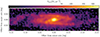 |
Fig. A.1. Molecular surface density map of NGC 253 derived from CO(2–1) emission. |
Appendix B: Star formation surface density
In Table B.1 we show coefficients used to compute the star formation surface density, whose map we show in Figure B.1.
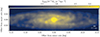 |
Fig. B.1. Star formation surface density map of NGC 253 using Herschel data. |
Coefficient for the calculation total infrared surface density (Equation 3, Section 2.4) taken from Galametz et al. (2013).
Appendix C: Spectral decomposition using SCOUSE
In our work, we use the Semi-automated multi-COmponent Universal Spectral-line fitting Engine (SCOUSE) (Henshaw et al. 2016, 2019), which is the spectral decomposition algorithm that defines where the line is located within the spectrum and describes such lines using Gaussian fitting. SCOUSE consists of four steps. In the first step, we define a spatial area over which we want to fit the spectra by creating a grid of macro pixels called Spectral Averaging Areas (SAAs). The size of a SAA is a free parameter. In our case, each SAA contains 4 pixels. The spectrum of each SAA represents the averaged spectrum of all the spectra within pixels contained in the SAA. In the second phase, SCOUSE fits each SAA’s spectrum and suggests a model solution assuming the Gaussian line profile. The model solution within each SAA consists of the detected number of Gaussian components and the fitting parameters: the amplitude, the centroid velocity, and the line width. In case when SCOUSE cannot find a proper solution for a fit, the user can manually change the requested signal-to-noise ratio in order for fitting parameters to converge or fit the respective spectrum manually by selecting the location of the spectral line within the spectrum, its peak, and the brightness temperature at which the spectrum reaches the 50 % of its peak. After completing the second phase, SCOUSE has a model solution of each SAA’s spectrum and uses these to fit pixels within each SAA. In the third phase, the user checks the SCOUSE’s model solutions for each pixel. Like the second phase, the user can change the number of Gaussian components and their fitting parameters. The location of each pixel in the map and SCOUSE solutions for their spectrum are saved in the textual file in the final, fourth phase.
All Tables
Coefficient for the calculation total infrared surface density (Equation 3, Section 2.4) taken from Galametz et al. (2013).
All Figures
|
Fig. 1. Composite image of NGC 253, its environments, and the 86–101 GHz spectrum taken with ALMA ACA. Top panel: NGC 253 composite (RGB and Hα) image (credits: Terry Robinson). The overlaid dashed gray rectangle shows the total u − υ coverage consisting of 25 pointing mosaic obtained by the ACA 7-m for this work. We indicate dynamical environments present in the disk of NGC 253: the center, bar, ring, and spiral arms (Querejeta et al. 2021). Bottom panel: observed spectrum taken toward the center of NGC 253. Our observations cover frequencies from 85.7 to 101.5 GHz. The term spectral window i (i takes values from 1 to 4) is abbreviated as spwi, and we mark all detected molecular emission lines. |
| In the text | |
|
Fig. 2. HCN and CO(2–1) moment maps. Top row: HCN(1–0) moment maps: integrated intensity map (left), centroid velocity map (middle), and velocity dispersion (right). The beam size of 22″ is shown in the left corner of each panel. Bottom row: CO(2–1) moment maps, in the same order as for HCN(1–0). CO(2–1) is convolved to a beam size of 22″, and regrided to match the grid of HCN data. The black line shows the outline of the HCN emission from the top panels. We fix the colorscale for each moment map to highlight the differences and similarities in HCN and CO(2–1) emission. All maps are rotated so that the x- and y-axis show the angular distance from the NGC 253’s minor and major axis (see Table 1). |
| In the text | |
|
Fig. 3. HCN-integrated intensity as a function of the galactocentric radius. The colored, filled points represent pixels with a signal-to-noise ratio of three and above, whereas open points have a signal-to-noise ratio lower than three. |
| In the text | |
|
Fig. 4. Radial distribution of the HCN/CO(2–1) intensity ratio across NGC 253. Sight lines are color-coded based on the environment. We show points with a signal-to-noise ratio above three in intensity and the peak brightness temperature. A small panel in this figure shows the distribution of the HCN/CO(2–1) line intensity ratio per environment in NGC 253: the center, bar, ring, spiral arms, and disk. The mean line ratio measured in each environment is shown as a horizontal line. |
| In the text | |
|
Fig. 5. HCN spectrum across NGC 253. Left: map of NGC 253 showing the number of velocity components in HCN emission across each pixel derived from SCOUSE. Right: example of HCN spectra from each environment shown in Figure 1 and from colored points on the left panel. The dashed black lines show each Gaussian velocity component derived from the SCOUSE spectra decomposition analysis (Henshaw et al. 2016, 2019). |
| In the text | |
|
Fig. 6. Results from the SCOUSE decomposition. Here, we show Gaussian fit parameters: peak brightness temperature (first row), centroid velocity (second row), number of components (third row), and velocity dispersion (bottom row) derived from SCOUSE. The left column shows the results from decomposing the HCN emission, whereas the right column shows output parameters computed for the CO(2–1) emission. We show results for each environment. Distribution for HCN emission along the disk is represented as a circle since there was no converging fits. |
| In the text | |
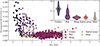 |
Fig. 7. Same as in Figure 4, but the HCN/CO(2–1) intensity ratio was calculated using SCOUSE. |
| In the text | |
|
Fig. 8. Component-by-component comparison between the HCN (y-axis) and CO(2–1) (x-axis) velocity dispersion derived from spectral decomposition using SCOUSE. We color-coded each point by the environment. The diagonal, solid black line shows a 1:1 ratio between the x- and y-axis. |
| In the text | |
|
Fig. 9. Decomposed HCN/CO(2–1) intensity (y-axis) and the CO(2–1) velocity dispersion (x-axis). We color-coded each point by the environment, similar to in Figure 8. |
| In the text | |
|
Fig. 10. SFR/HCN luminosity ratio as a proxy for the star formation efficiency of dense molecular gas as a function of Σmol. Points are color-coded according to their environments. Vertical dashed lines show the surface density thresholds of ∼10 M⊙ pc−2 and ∼200 M⊙ pc−2, previously defined in Bigiel et al. (2008). The horizontal shaded region shows a range of 400 − 500 L⊙/M⊙. |
| In the text | |
|
Fig. 11. Ability of dense gas to form stars, traced by the IR/HCN luminosity ratio, as a function of the HCN velocity dispersion measured from spectral decomposition analysis. We color-coded each point by the environment. |
| In the text | |
|
Fig. 12. HCN spectrum taken along the minor axis. Left: bar sight lines in NGC 253. We label major and minor axes. Colored points are sight lines showing enhanced HCN/CO(2–1) emission in the direction of the SW streamer (Walter et al. 2017) and that contribute to the bimodality seen in Figure 4. Colors correspond to their HCN/CO(2–1) intensity ratio shown in the colorbar. Right: HCN spectra toward the data points located along the minor axis in NGC 253 shown on the left. Each spectrum is colored by the HCN/CO(2–1) ratio shown on the colorbar. All these data points are located along the SW streamer (Walter et al. 2017). The black dashed line shows NGC 253 systemic velocity of 243 km s−1 (see Table 1). The black solid line represents the υlsr = 200 km s−1 velocity at which Walter et al. (2017) observed the outflowing component in CO(1–0) emission. |
| In the text | |
|
Fig. 13. Position–velocity diagram (pυ) of the HCN emission in NGC 253. The y-axis shows the centroid velocities from the spectral decomposition, and the x-axis shows the angular distances from the minor axis of NGC 253. We color-coded points by their HCN/CO(2–1) ratio derived from SCOUSE, and the size of each point corresponds to the HCN velocity dispersion. |
| In the text | |
|
Fig. 14. Summary of previous dense gas studies. Top left: literature overview of the infrared luminosity (a proxy for the star formation rate) as a function of the HCN luminosity (a proxy for dense molecular gas), that is, the Gao and Solomon relation (Gao & Solomon 2004). We show measurements of whole galaxies and their centers at a few kpcs (see the legend in the upper and the lower-left of the panel), Milky Way clouds (a few pc scales - see legend on the bottom right), including measurements across NGC 253 (this work - see the legend on the right central part) (Jiménez-Donaire et al. 2019). The dark red line shows a 500 M⊙/L⊙ which corresponds to a upper limit reported in Scoville & Wilson (2004) and Thompson et al. (2005). Top right: same as in the left panel, but we are now showing SFEdense, traced by the IR/HCN luminosity ratio on the y axis. In both panels, the black solid line shows the mean IR/HCN luminosity ratio measured by the EMPIRE survey (Jiménez-Donaire et al. 2019). Black dashed lines show the 1σ RMS scatter of ±0.37 dex in units of L⊙/(K km s−1 pc2). Bottom row: zoomed-in view of the field from Figure 14, where we show NGC 253 sight lines, points from the nearby starburst galaxy M 82 (Kepley et al. 2014), the merging system of the Antennae galaxies (Bigiel et al. 2015), and a sample of LIRGs and ULIRGs (García-Burillo et al. 2012). Axes are the same as of the panels at the top row. Data points from Kepley et al. (2014) have different shades of gray that corresponds to the distance to the center of M 82, where the darkest points have the smallest galactocentric distances. |
| In the text | |
|
Fig. A.1. Molecular surface density map of NGC 253 derived from CO(2–1) emission. |
| In the text | |
|
Fig. B.1. Star formation surface density map of NGC 253 using Herschel data. |
| In the text | |
Current usage metrics show cumulative count of Article Views (full-text article views including HTML views, PDF and ePub downloads, according to the available data) and Abstracts Views on Vision4Press platform.
Data correspond to usage on the plateform after 2015. The current usage metrics is available 48-96 hours after online publication and is updated daily on week days.
Initial download of the metrics may take a while.