| Issue |
A&A
Volume 691, November 2024
|
|
|---|---|---|
| Article Number | A285 | |
| Number of page(s) | 24 | |
| Section | Extragalactic astronomy | |
| DOI | https://doi.org/10.1051/0004-6361/202451147 | |
| Published online | 20 November 2024 | |
A survey of extremely metal-poor gas at cosmic noon
Evidence of elevated [O/Fe]
1
INAF – Osservatorio Astronomico di Trieste, Via G. B. Tiepolo 11, I-34143 Trieste, Italy
2
Dipartimento di Fisica G. Occhialini, Università degli Studi di Milano Bicocca, Piazza della Scienza 3, I-20126 Milano, Italy
3
IFPU – Institute for Fundamental Physics of the Universe, Via Beirut 2, I-34151 Trieste, Italy
4
Centre for Extragalactic Astronomy, Durham University, South Road, Durham DH1 3LE, UK
5
Institute of Astronomy, University of Cambridge, Madingley Road, Cambridge CB3 0HA, UK
6
The Observatories of the Carnegie Institution for Sciences, 813 Santa Barbara Street, Pasadena, CA, USA
⋆ Corresponding author; This email address is being protected from spambots. You need JavaScript enabled to view it.
Received:
17
June
2024
Accepted:
11
September
2024
Abstract
Aims. We aim to study the high-precision chemical abundances of metal-poor gas clouds at cosmic noon (2 < z < 4) and investigate the associated enrichment histories.
Methods. We analyze the abundances of four newly discovered metal-poor gas clouds utilizing observations conducted with Keck/HIRES and VLT/UVES. These systems are classified as very metal-poor (VMP), with [Fe/H] < −2.57, and one system qualifies as an extremely metal-poor (EMP) Damped Lyman-α (DLA) system with [Fe/H] = −3.13 ± 0.06. In combination with new high-resolution data of two previously known EMP DLAs and 2 systems reported in the literature, we conduct a comprehensive analysis of eight of the most metal-poor gas clouds currently known. We focus on high-precision abundance measurements using the elements: C, N, O, Al, Si, and Fe.
Results. Our findings indicate increasing evidence of elevated [O/Fe] abundances when [Fe/H] < −3. EMP DLAs are well-modeled with a mean value of [O/Fe]cen = +0.50 ± 0.04 and an intrinsic scatter of σint[O/Fe] = 0.13-0.04+0.06. While VMP DLAs are well-modeled with [O/Fe]cen = +0.40 ± 0.02 and σint, [O/Fe] = 0.06 ± 0.02. We further find tentative evidence of a redshift evolution of [C/O] across these most metal-poor DLAs with lower redshift systems showing elevated [C/O] ratios. Using the measured abundances, combined with a stochastic chemical enrichment model, we investigate the properties of the stellar population responsible for enriching EMP gas at cosmic noon. We find that the chemistry of these systems is best explained via the enrichment of just two massive progenitors, N⋆ = 2 ± 1, that ended their lives as core collapse SNe with a typical explosion energy Eexp = (1.6 ± 0.6)×1051 erg. These progenitors formed obeying a Salpeter-like power-law IMF, where all stars of mass greater than Mmax = 32-4+10M⊙ collapse directly to black holes and do not contribute to the metal enrichment.
Key words: stars: Population II / stars: Population III / quasars: absorption lines
© The Authors 2024
 Open Access article, published by EDP Sciences, under the terms of the Creative Commons Attribution License (https://creativecommons.org/licenses/by/4.0), which permits unrestricted use, distribution, and reproduction in any medium, provided the original work is properly cited.
This article is published in open access under the Subscribe to Open model. This email address is being protected from spambots. You need JavaScript enabled to view it. to support open access publication.
1. Introduction
Tracing chemical evolution from the Cosmic Dawn (15 < z < 30) to the present day unequivocally begins with the first generation of Population III (Pop. III) stars (Bromm & Yoshida 2011). Understanding the properties of these stars is essential to unveiling the first instances of chemical enrichment and the origin of chemical elements in the Universe (Kobayashi et al. 2020; Klessen & Glover 2023).
Within the current cosmological framework, the primordial Universe was primarily composed of hydrogen, helium, and trace amounts of lithium. The creation of the first metals began with the birth of the first stars; the cores of these Pop. III stars were the dominant source of heavy elements at this epoch.
Current state-of-the-art simulations of Pop. III star formation suggest that these stars may have had a relatively high characteristic mass (M > 10 M⊙) and were therefore short-lived (Bromm & Yoshida 2011). Thus, the probability of directly detecting Pop. III stars in the local Universe is low. However, when the first stars ended their lives, they enriched the surrounding environment with the first instances of metals. The resulting abundances of these metals depend directly on the properties of the first stars (e.g., their initial mass function; IMF, explosion energy, rotation properties etc.). Thus, by identifying the unique chemical fingerprint of the first stars one may indirectly recover some of their properties. Typically this fingerprint is searched for via the metal-poor stars in the halo of the Milky Way (MW) and its surrounding dwarf galaxies (e.g., Bond 1980; Beers et al. 1985; Aoki et al. 2006; Frebel et al. 2005; Frebel & Norris 2015; Hartwig et al. 2018, 2023; Ishigaki et al. 2018; Starkenburg et al. 2017; Arentsen et al. 2020; Vanni et al. 2023). It has also been realised that metal-poor gas reservoirs at high redshifts can be used to search for this fingerprint (Erni et al. 2006; Pettini et al. 2008; Penprase et al. 2010; Cooke et al. 2017; Welsh et al. 2019, 2023; Nuñez et al. 2022).
These gas reservoirs are typically detected as absorption along the line-of-sight toward unrelated background quasars. The highest column density gas reservoirs, whose column density of neutral hydrogen exceeds log10(N(H I)/cm−2)≥20.3 are known as Damped Lyα systems (DLAs; see Wolfe et al. 2005 for a review). The significant amount of neutral hydrogen in these gas clouds shields the relatively few metals from ionizing photons. As a result, most elements associated with the neutral gas are in a single dominant ionization stage. These dominant ionization stages are known based on the relative excitation energies with respect to that of hydrogen; ionization corrections are therefore negligible, provided that the abundance of the dominant ion stage of each metal can be measured. Thus, these DLAs are arguably some of the best astrophysical environments to precisely determine chemical abundances in the early Universe. Also of interest are the slightly lower column density absorbers known as sub-DLAs. These reservoirs have a neutral H I content between 19.0 < log10(N(H I)/cm−2) < 20.3 and may intersect partially ionized gas.
Crucially, gas reservoirs detected in absorption allow us to study low density structures in the early Universe that are otherwise challenging to detect. They are an invaluable tool to study the evolution of metals across cosmic time. At redshift z ∼ 3, approximately 60% of observed metals are found in low-ionization gas often associated with DLAs. This fraction increases at higher redshifts (Péroux & Howk 2020).
Of particular interest is the evolution of some of the most abundant chemical elements (e.g., C, O, N, Ne, and Si) alongside that of iron-peak elements (e.g., Fe, Ni, and Zn). Historically, searches for signatures of the first stars have focused on discovering the most iron-poor environments. In these investigations, it is typical to exclusively consider systems that are at least extremely metal-poor (EMP). EMP systems are defined as having an iron abundance that is between 1/10 000th and 1/1000th of the solar abundance (Beers & Christlieb 2005). This is often expressed as1 −4 < [Fe/H] < −3. Systems with an [Fe/H] abundance between −3 < [Fe/H] < −2 are classified as being very metal-poor (VMP).
The behavior of [α/Fe] as a function of the Fe-metallicity is an informative probe of chemical enrichment2. The evolution of this relative abundance ratio can indicate the onset of enrichment from Type Ia supernovae (SNe) (Tinsley 1979; Wheeler et al. 1989). This was first detected within the MW whose constituent stars exhibit a plateau in the [α/Fe] abundance ratio at low metallicities. This persists until [Fe/H] ∼ −1, when the [α/Fe] abundance begins to decline (Matteucci & Brocato 1990; Matteucci 2003; Edvardsson et al. 1993; Ishigaki et al. 2012). Since Type Ia SNe predominantly produce Fe-peak elements, this decline in [α/Fe] corresponds to the onset of enrichment from long-lived, low-mass stars that left the main sequence as white dwarfs. Prior to the enrichment from these low mass stars, it is the IMF-weighted abundances of the more massive and, consequently, short-lived stars that are being observed. These massive stars are rich in both α- and Fe-peak elements. Once the supply of massive stars is exhausted, there is no way to replenish the α-abundances (without a subsequent burst of star-formation).
The stellar populations of nearby satellite dwarf spheroidal galaxies (dSphs) also exhibit this so-called “α-knee”. In these more metal-poor environments, the knee occurs at lower metallicities than in the MW (Tolstoy et al. 2009; Kirby et al. 2011). Sculptor and Fornax show a decline in [α/Fe] at [Fe/H] = −1.8 and [Fe/H] = −1.9, respectively (Starkenburg et al. 2013; Hendricks et al. 2014; Hill et al. 2019). This behavior has also been characterised for metal-poor DLAs at z ∼ 3 (Cooke et al. 2015; Velichko et al. 2024). The metallicity of the “α-knee” across the metal-poor DLA population is found to be [Fe/H] ∼ −2. While this knee is observed across a sample of objects, rather than an individual galaxy, it is still an informative measure of chemical enrichment.
Oxygen is the most abundant metal in the Universe (Lodders 2019; Magg et al. 2022). It is a key α-element for investigating chemical evolution. VMP DLAs exhibit a plateau in their [O/Fe] abundance at [O/Fe] ≃ +0.4 (Cooke et al. 2011). This suggests that the DLAs in this metallicity regime were enriched by a similar population of stars drawn from the same IMF. This is comparable to the IMF-weighted abundance of elements observed across galaxies that show an α-knee. Notably, the [Fe/H] position of the knee observed for both Sculptor and Fornax coincides with the region in which the DLA abundances appear to initially plateau ([Fe/H] ≲ −2).
At lower metallicities, bordering on the EMP regime, this plateau in [O/Fe] appears to break down. Previous works indicate that this ratio is enhanced relative to the higher metallicity systems. This could be a signature of enrichment by a generation of metal-free stars (e.g., Heger & Woosley 2010). Indeed, theoretical works that explore the Pop. III signature in the intergalactic medium (IGM) at z ∼ 3 find that the imprint of the first stars may be seen in gas reservoirs with [Fe/H] < −3 that additionally show an [O/Fe] enhancement (Kirihara et al. 2020). In fact, some models indicate that the entire abundance patterns observed across metal-poor DLAs at z ∼ 3 are consistent with Pop. III enrichment (Maio & Tescari 2015; Webster et al. 2015).
Discerning the true behavior of [O/Fe] in the EMP regime is challenging due to the typical size of the associated uncertainties (> 0.1 dex) compared to the expected strength of the enhancement (variable depending on the underlying IMF). These challenges can be overcome through deep observational programs curated for absorbers of interest. Recent work, led by this group, has highlighted the value in such a program when targeting DLAs between 2 < zabs < 4. In particular, our observations and subsequent analysis of an opportunely placed DLA in the [O/Fe]-[Fe/H] parameter space strengthened the observed signature of an elevated [O/Fe] ratio in the EMP regime compared to the VMP regime with a significance of ∼2σ (Welsh et al. 2022). This was further reaffirmed by our latest observations and analysis of the most metal-poor DLA currently known (Cooke et al. 2017; Welsh et al. 2023).
Indeed, this previous work also highlights the value of each newly discovered EMP DLA when investigating early chemical enrichment and searching for the chemical fingerprint of the first stars. Discovering this signature is one of the key science goals of the next generation of telescope facilities (D’Odorico et al. 2023).
Notably, metal-poor systems, particularly EMP DLAs, make up a small fraction of the overall number of absorbers discovered at 2 < z < 4 (known as cosmic noon; Péroux & Howk 2020). When looking at statistical surveys, they are often not detected (Rafelski et al. 2012; Lehner et al. 2022). However, they can be found through dedicated surveys, as shown in Pettini et al. (2008) and Penprase et al. (2010). Indeed, there has been increasing interest in studying metal-poor DLAs with high resolution optical spectrographs for more than two decades (e.g., Molaro et al. 2000; Dessauges-Zavadsky et al. 2001; O’Meara et al. 2001; Erni et al. 2006; Petitjean et al. 2008; Cooke et al. 2011, 2014; Dutta et al. 2014; Morrison et al. 2016; Berg et al. 2024). Cosmic noon is the only epoch thus far where completely chemically pristine gas has been detected (Fumagalli et al. 2011; Robert et al. 2019). It is also the epoch in which both the strongest metal absorption features and the associated Lyα absorption (rest frame UV) fall in the optical wavelength range. With the ever-increasing number of quasars being found at redshift z > 6, it may also become possible to discover pristine gas closer to the epoch of the Cosmic Dawn by searching for proximate absorption line systems (e.g., Bañados et al. 2019; Sodini et al. 2024).
Here we present the results of our latest survey of metal-poor gas clouds at cosmic noon and investigate their associated chemical abundance pattern using high resolution echelle spectroscopy. Specifically, we report the discovery of four new metal-poor systems. One of these newly discovered systems is a bonafide EMP DLA with [Fe/H] = −3.13 ± 0.06. Another system is on the cusp of this regime with [Fe/H] = −3.00 ± 0.12 and the remaining two systems are found to be VMP. Together with these new discoveries, we summarize our ongoing program designed to obtain new data of known EMP DLAs. We present the results of this bespoke program in the form of new high resolution data of two previously known EMP DLAs. Combined with the work presented in Welsh et al. (2022, 2023), we form a sample of eight of the most metal-poor high column density absorbers at cosmic noon and use these data to determine the precise chemical abundance patterns in this regime. In particular, we focus on the chemical evolution of [O/Fe].
This paper is organised as follows. Section 2 describes our targets and the observations. Section 3 details the data reduction and fitting procedure process. In Section 4, we present the details of our sample and our data. We analyze the chemical abundances in Section 5 and consider possible impacts of physical processes in Section 6. In Section 7, we discuss these results and draw comparisons with other works, before drawing overall conclusions and suggesting future work in Section 8.
2. Observations
The data presented in this paper are either the first high-resolution observations of the DLA or we have obtained additional high-resolution observations designed to pin down the Fe II column density with increased precision. A summary of the observations can be found in Table 1. These data were taken with either the Ultraviolet and Visual Echelle Spectrograph (UVES; Dekker et al. 2000) at the European Southern Observatory (ESO) Very Large Telescope (VLT) or the High Resolution Echelle Spectrometer (HIRES; Vogt et al. 1994) at the Keck observatory. Our latest observations of the individual systems are described in turn. Unless otherwise stated, all observations were carried out with a 0.8″ slitwidth and 2 × 2 binning during readout.
Journal of observations associated with our sample.
2.1. Known EMP DLA program
2.1.1. J0140−0839
The proximate DLA found toward the QSO SDSS J014049.18−083942.50 (hereafter J0140−0839), with mr = 17.75, was first identified using data from the Sloan Digital Sky Survey (SDSS) (Prochaska et al. 2008). High resolution echelle spectroscopic data were then taken with UVES (R ∼ 40 000) and presented in Ellison et al. (2010). Based on these data and the subsequent reanalysis presented in Cooke et al. (2011), this DLA was identified as one of the most Fe-poor DLAs known with an estimated Fe abundance of [Fe/H] = −3.45 ± 0.24. In this paper, we present an additional ∼16 hours of VLT/UVES data taken during observing periods P105 to P108. Approximately 8 hours of observations were taken with the 437+760 setup and a further ∼8 hours were taken with the 437+860 setup, both executed as 10 × 3000 s exposures.
2.1.2. J1358+0349
The DLA toward the quasar QSO SDSS J135803.97+034936.01 (hereafter J1358+0349) with mr = 18.64 was, at one point, the most metal-poor DLA known. It has been observed extensively to study the primordial abundance of deuterium (Cooke et al. 2016). Consequently, previous observations focused on blue wavelengths. We present new VLT/UVES data that focus on red wavelengths and cover the previously unobserved Fe IIλ2344 and Fe IIλ2382 features. These intrinsically strong absorption lines fall at red wavelengths that are commonly impacted by telluric features. To accommodate for this potential contamination, we observed a telluric standard star (using an identical instrument setup) alongside every exposure on target. This allows for the accurate removal of telluric features from the spectrum extracted from each exposure. The process of telluric removal can be found in Appendix A alongside additional tests. The latest data were taken with the 390+760 setup and executed as 8 × 2700 s exposures. All exposures were followed with a 3 s exposure of a nearby A0V star, HD 126129. For the details of the archival UVES and HIRES data we refer the reader to Cooke et al. (2016).
2.2. Survey for new systems
In addition to our follow-up survey to study all known EMP DLAs with high-precision, we present the latest results from our ongoing search for new DLAs in the EMP regime. These DLAs were initially identified from SDSS spectroscopic data using the Parks et al. (2018) DLA catalog. Using this catalog, we identified a sample of candidate DLAs that appeared to be at least VMP. We sought additional data of these targets through dedicated observations with an intermediate resolution spectrograph; specifically, the recently decommissioned Intermediate-dispersion Spectrograph and Imaging System (ISIS) at the 4.2 m William Herschel Telescope (WHT). The resolution of these follow-up data was sufficient to identify the most promising candidates for further observations with a high resolution echelle spectrograph. In particular, we focus on absorption line systems that would be of interest for studies of near-pristine gas. Thus, we acquired VLT/UVES or Keck/HIRES data to pin down the detailed chemistry and kinematics of these absorption line systems. The details of these observations are below. In all cases, we are reporting the identified absorber for the first time. Further, these are the first observations of each system obtained with sufficient resolution to resolve the cloud properties.
2.2.1. J0239−0649
Based on observations with VLT/UVES, we have identified the DLA toward the zem = 2.49 mr = 18.66 QSO SDSS J023936.99−064931.15 (hereafter J0239−0649) at zabs = 2.416. We observed the sightline using the 437+760 setup for a total of 18 000 s. These observations were executed as 6 × 3000 s exposures and reach a final combined S/N near the bluest accessible Fe II feature of S/N = 11.
2.2.2. J1147+5034
Through observations with Keck/HIRES, we have identified the proximate DLA toward the zem = 2.52 mr = 19.45 QSO SDSS J114745.03+503446.8 (hereafter J1147+5034) with zabs = 2.519. This sightline was observed using the red cross disperser, a cross disperser angle of 0.43 degrees, and an echelle angle of 0.58 degrees combined with a slit length of 7.0″ and a slit width of 0.861″ (decker C1). The measured resolution of these data is R ≃ 50 000 (≡6 km s−1 full width at half maximum; FWHM). We executed our observations as 5 × 3600 s exposures. With these data, we reach a final combined S/N near the accessible Fe II feature of S/N = 22.
2.2.3. J2150+0331
The third newly observed DLA is found toward the zem = 2.79 mr = 19.12 QSO SDSS J215037.68+033131.39 (hereafter J2150+0331) at zabs = 2.697. This sightline was observed with VLT/UVES in P110 using the 437+760 setup for a total of 30 000 s executed as 10 × 3000 s exposures. With these data, we reach a final combined S/N near the accessible Fe II feature of S/N = 11.
2.2.4. J2308+0854
The final absorption line system presented in this paper is found toward the zem = 2.77 mr = 19.40 QSO SDSS J230844.19+085442.28 (hereafter J2308+0854) at zabs = 2.768. This sightline was observed with VLT/UVES throughout P108 using the 390+564 setup as well as the 437+760 setup. In total, we obtained 12 × 3000 s exposures; 3 of these were executed with the 390+564 setup with the primary aim of observing the absorption due to neutral hydrogen. The remaining 9 exposures were executed using the 437+760 setup to cover the majority of the metal lines of interest. With these data, we reach a final combined S/N near the accessible Fe II feature of S/N = 19.
3. Data reduction and analysis
3.1. Data reduction
The HIRES data were reduced using two different software packages. For data taken prior to 2022, the Hires REDUX3 reduction pipeline was used (Bernstein et al. 2015). For data taken after this epoch, the data were reduced with the PypeIt4 reduction pipeline (Prochaska et al. 2020). The ESO data were all reduced with the EsoRex reduction pipeline. Each pipeline includes the standard reduction steps of subtracting the detector bias, locating and tracing the echelle orders, flat-fielding, sky subtraction, optimally extracting the 1D spectrum, and performing a wavelength calibration. The data were converted to a vacuum and heliocentric reference frame.
Finally, we combined the individual exposures of each DLA using UVES_POPLER56 (Murphy et al. 2019). This corrects for the blaze profile, and allowed us to manually mask cosmic rays and minor defects from the combined spectrum. When combining these data we adopted a pixel sampling of 2.5 km s−1. In some cases, there are differences in resolution across the available data associated with a given DLA. This is a result of observations being taken with different slitwidths. When this was the case, we combined and analyzed the data separately. We further note that some of these data were taken > 10 years apart. To avoid issues associated with combining data of quasars with significant continuum variability, we similarly treated data taken across substantially different periods (i.e., in excess of 2 years) separately.
3.2. Analysis approach
Using the Absorption LIne Software (ALIS) package7 – which uses a χ-squared minimization procedure to find the model parameters that best describe the input data – we simultaneously analyzed the full complement of high S/N and high spectral resolution data currently available for each DLA. We modeled the absorption lines with Voigt profiles, which consisted of three free parameters: a column density, a redshift, and a line broadening parameter. We assumed that all lines of comparable ionization level have the same redshift, and any absorption lines that are produced by the same ion all have the same column density and broadening prescription. The total broadening of the lines includes a contribution from both turbulent and thermal broadening. The turbulent broadening is assumed to be the same for all absorption features, while the thermal broadening depends inversely on the square root of the ion mass; thus, heavy elements (e.g., Fe) will exhibit absorption profiles that are intrinsically narrower than the profiles of lighter elements, (e.g., C). There is an additional contribution to the apparent line broadening due to the instrument; we approximated the instrument broadening function using a Gaussian with a width that depends on the instrument setup. For the HIRES and UVES data, the nominal instrument resolutions are vFWHM = 6.28 km s−1 (HIRES C1), vFWHM = 8.33 km s−1 (UVES slitwidth = 1″), and vFWHM = 7.3 km s−1 (UVES slitwidth = 0.8″). Finally, we note that we simultaneously fit the absorption and quasar continuum of the data. We modeled the continuum around every absorption line as a low-order Legendre polynomial (typically of order 3). We assumed that the zero-levels of the sky-subtracted UVES and HIRES data do not depart from zero8. This approach ensures that the final ion column densities and their associated errors capture the additional correlated uncertainties associated with the localised continuum model.
In the following section, we discuss our sample in detail and present the results of this profile fitting for each DLA. We first attempted to use the full complement of available data to determine the gas temperature and turbulent broadening alongside the ion column densities. In the case of clouds with multiple components, it is not possible to assess the turbulent and thermal contribution to the overall Doppler broadening. Therefore, in these instances, we adopted cloud models that assume a temperature typically observed in H I dominated gas (Cooke et al. 2014; Noterdaeme et al. 2021). The range of temperatures we considered is T = (0.8 − 1.2)×104 K. If the resulting column densities were consistent within this temperature range, we report column densities and turbulent broadening under the assumption of T = 1 × 10⁴ K. We also adopt this approach if the turbulent motions of the gas are significantly dominant over the potential thermal contribution and if the level of saturation makes our fiducial approach untenable. This approach does not impact the derived column densities since the absorption features that are covered for the ions of interest are typically weak and unsaturated.
We present the column densities of all detected components in Tables 2–7 for each gas cloud. Here, and subsequently, the errors are given by the square root of the diagonal term of the covariance matrix calculated by ALIS at the end of the fitting procedure. To accommodate the presence of potentially ionised gas, we pay particular attention to the components that are traced by neutral oxygen since these should be tracing the predominantly neutral gas. For the case of complex systems, the components traced by both O and Fe are highlighted appropriately in the relevant figures. We adopt a strategy of marking the neutral components with red ticks. These are consistently also the strongest components. Indeed, when considering the chemistry of these clouds, we also restrict our analysis to the components traced by neutral gas.
Ion column densities of the DLA at zabs = 3.696621 ± 0.000002 toward the quasar J0140−0839.
Ion column densities of the DLA at zabs = 2.41623 toward the quasar J0239−0649.
4. Sample
In this section we present the details of our sample and the results of our line fitting procedure. The relative abundances of the DLAs in our sample will be discussed in Section 5 and are summarized in Table 8. Readers interested in the relative abundances of the sample, and not the details on individual systems, can refer to Section 5.
Metal abundances of our DLA sample.
4.1. Known EMP DLAs
Half of our sample is comprised of the four previously known EMP DLAs that we will now discuss in turn.
4.1.1. J0140−0839
Our latest analysis of J0140−0839 indicates that this absorption line system is best modeled by seven absorption features spread over ∼200 km s−1. The column densities of these components are presented in Table 2 alongside their individual redshifts and turbulent broadening. The reduced data and the associated model fit to these data are shown in Figure 1. The data in this figure are centred on the strongest component at zabs = 3.696621 ± 0.000002. We have refit the Lyα profile associated with this DLA. Given this latest model of the continuum, we find log10N(H I)/cm−2 = 20.81 ± 0.05.
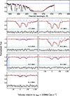 |
Fig. 1. Continuum normalized UVES data (black histograms) of the absorption features associated with the DLA at zabs = 3.69662 toward J0140−0819. The best-fitting model is shown with the red curves. The blue dashed line indicates the position of the continuum while the green dashed line indicates the zero-level. The ticks above the absorption features indicate the centre of the Voigt line profiles. The features of the strongest components are distinguished via red ticks while those of weaker components are shown in blue. These strongest components are also often associated with the predominantly neutral gas. The purple ticks indicate absorption features unrelated to the DLA. Below the zero-level, we show the residuals of this fit (black histogram) where the gray shaded band encompasses the 2σ deviates between the model and the data. The vertical blue shaded bands indicate the regions of the spectrum not included in the fit. Note that the full complement of available data were used in calculating the best-fit model, while we only show a selection of the data in this figure to showcase the model and the data. We also note that the y-axis scale is different in some panels to highlight the very weak absorption lines. |
While this is a seven component system, the cloud is dominated by the two strongest components. These strong components are indicated with red ticks in Figure 1. Indeed, the accessible Fe II features are the weak λ1260 and λ1608 features and they are both only detected for the two strongest components. Notably, this DLA remains one of the most Fe-poor systems currently known with [Fe/H] = −3.37 ± 0.06. This abundance ratio is now known with a three times greater precision compared to previous determinations. This was predominantly facilitated by the higher S/N data available near the Fe IIλ1608 feature. The associated [O/Fe] abundance is now known with four times greater precision. We find [O/Fe] = +0.45 ± 0.04 while it was previously determined to be [O/Fe] = +0.70 ± 0.19.
4.1.2. J0903+2628
The DLA found toward the quasar SDSS J090333.55+262836.3 (hereafter J0903+2628) is the most metal-poor DLA currently known (Cooke et al. 2017; Welsh et al. 2023). We recently acquired an additional 10 hours of echelle spectroscopic data on the associated quasar using Keck I/HIRESr. We refer the reader to these papers for details and we present the relevant abundances in Table 8.
4.1.3. J1001+0343
The DLA toward SDSS J100151.45+034301.4 (hereafter J1001+0343) is a previously known EMP DLA. The VLT/UVES data that facilitated the latest investigation of [O/Fe] are presented in Welsh et al. (2022). In summary, the latest data reduced the error associated with the [O/Fe] determination by a factor of three. We refer the reader to this work for further details. This earlier work highlights that the behavior of [O/Fe] in the EMP regime is more easily studied with high precision abundance determinations. Again, the relevant abundances are collected in Table 8. For the first time, we report the [Al/H] abundance of this system.
4.1.4. J1358+0349
J1358+0349 is another system that is best-modeled using multiple components. The reduced data and the associated model fit to these data are shown in Figure B.1 while the decomposed column densities of each component are presented in Table 3. The strongest O I component is located at zabs = 2.852871 ± 0.000002. As has been found in previous works, this DLA has a deceptively complex kinematic structure. It cannot be well-modeled assuming that the components share the same relative abundances of metals.
Two components are traced by both O and Fe. These are marked with red ticks in Figure B.1. The central C, Al, Si, and Fe features follow the same three components. The main O I structure is also traced by three components. We note that the first two O I components are consistent with those found for the singly ionised features. However, the third component shows a small offset to that of the third component traced by C, Al, Si, and Fe. There is a further (fourth) O I component that is offset from the central cloud at v ∼ +80 km s−1; this is also traced by Si II.
Despite this complexity, we can report the total column density of iron for this system using three Fe II features (specifically λ1608, λ2344, and λ2382) that have different oscillator strengths. With these data, we find [Fe/H] = −3.45 ± 0.04. This is based on the Fe II column densities of the two components also traced by O I. The associated [O/Fe] abundance is [O/Fe] = +0.60 ± 0.06. This is consistent with previous observations and the associated errors have been reduced by a factor of three. We cannot improve on the neutral hydrogen column density log10N(H I)/cm−2 = 20.524 ± 0.006 reported in Cooke et al. (2016).
4.2. New high column density absorbers
We now present the data associated with the newly discovered high column density absorbers. As previously discussed, these absorbers were first identified as potentially metal-poor systems through SDSS data and the Parks et al. (2018) DLA catalog. They remained promisingly metal-poor when observed with an intermediate resolution spectrograph. These data were collected with WHT/ISIS (recently decommisioned in favor of the WHT Enhanced Area Velocity Explorer (WEAVE) survey instrument; Dalton et al. 2012). The targets that appeared to be the most metal-poor based on the ISIS data were then followed up with a high resolution echelle spectrograph capable of resolving the detailed structure of the absorption lines, thereby allowing us to pin down the underlying cloud model and component column densities with confidence.
4.2.1. J0239−0649
The absorber toward J0239−0649 is best modeled with one gaseous component at zabs = 2.416233 ± 0.000001 for all detected species. The detected features of the light atomic elements C and O are unfortunately saturated. Our analysis is restricted to those with the largest oscillator strengths. The weaker features are covered by our observations but are heavily blended with unrelated absorption. Given this saturation, there is not enough information in these data to constrain the turbulent and thermal broadening of the gas simultaneously. Instead, we explore the cloud models that assume a temperature typically observed in H I dominated gas (as discussed in Section 3.2). Under the assumption T = 1 × 10⁴ K, we find that the turbulent velocity contribution is b = 3.6 ± 0.2 km s−1. The data, along with the best-fitting model are presented in Figure B.2, while the corresponding column densities are listed in Table 4. Despite the saturation of the C II and O I lines, one can still obtain reliable abundance measures by using the Si II and Fe II features, that cover a range of fλ values, to pin down the cloud model. There is an additional uncertainty associated with fitting modestly saturated lines since the observed line profiles are less visibly impacted by changes in column density. This can be minimised by fitting all of the metal lines simultaneously.
We measure [Fe/H] = −2.64 ± 0.06 placing it firmly in the VMP regime. We find that the total column density of neutral hydrogen is log10N(H I)/cm−2 = 20.10 ± 0.05. We do not detect appreciable absorption from any Fe-peak elements beyond Fe (such as Cr, Ni, or Zn). However, we tentatively detect N I via the λ1200 triplet with a ∼2σ confidence. This suggests [N/O] ≃ −1.2 while [N/H] = −3.33 ± 0.16. This DLA is therefore found to be inline with the [N/α] plateau observed at [N/α]= − 1.45 ± 0.05 for DLAs with low [N/H] abundances (Centurión et al. 2003; Zafar et al. 2014). It is also in support of works that find that the distribution of [N/O] measured across high redshift absorbers shows a high level of dispersion (Pettini et al. 2008; Petitjean et al. 2008; Vangioni et al. 2018). Though, we note that the quality of these data are only sufficient to report a marginal N detection. Thus, we defer to future observations for further analysis.
4.2.2. J1147+5034
The DLA toward J1147+5034 is best modeled by one gaseous component at zabs = 2.518882 ± 0.000001. This gas cloud has a temperature of T = (1.7 ± 0.8)×104 K and a turbulent doppler parameter of b = 3.65 ± 0.91 km s−1. The data, along with the best-fitting model are presented in Figure B.3, while the corresponding column densities are listed in Table 5. We find that log10N(H I)/cm−2 = 20.23 ± 0.01 and [Fe/H] = −3.13 ± 0.06. This is the most metal-poor newly discovered DLA from this survey. It is additionally the lowest redshift EMP DLA discovered to date with an absorption redshift zabs = 2.519.
As can be seen in the top panel of Figure B.3, these data provide a clean detection of the Si IIIλ1206 feature. Given that this system has a H I column density that lies near the border of being classified as a DLA, we can use the successive ion ratio Si III/Si II to investigate the potential need for ionization corrections (as done in Section 6.1). We also detect C IV that is coincident in velocity space with the low ionization absorption (as reported in Table 5).
4.2.3. J2150+0331
The absorber toward J2150+0331 is best modeled with one gaseous component at zabs = 2.697125 ± 0.000002. The data, along with the best-fitting model are presented in Figure B.4, while the corresponding column densities are listed in Table 6. The broadening of this absorption line system is consistent with being entirely dominated by its thermal motions with a temperature of T = (1.6 ± 0.4)×104 K. The narrow absorption features of this system combined with its metal paucity make it an ideal system for isotopic abundance studies with the ultrastable spectrograph ESPRESSO (Welsh et al. in prep.).
We find that log10N(H I)/cm−2 = 19.68 ± 0.05. This is the lowest H I column density system discovered by our program so far. The column density is 4× lower than that of a bonafide DLA. We detect C IV, as reported in Table 6, that is minimally offset from the central component. Based on the Fe II transitions λ1260, λ1608, and λ2382 and the H I column density9, we infer an iron abundance [Fe/H] = −2.57 ± 0.08.
4.2.4. J2308+0854
The absorber toward J2308+0854 is best modeled with one gaseous component at zabs = 2.768607 ± 0.000006 with a turbulence of b = 19 ± 3 km s−1. During the analysis, we found that the total Doppler broadening of this gas cloud is dominated by turbulent motions. Thus, we adopt a temperature of T = 1.0 × 10⁴ K, although, even with this temperature, the kinematics are completely dominated by the turbulent motions. The data, along with the best-fitting model are presented in Figure B.5, while the corresponding column densities are listed in Table 7. We find that log10N(H I)/cm−2 = 19.95 ± 0.05 and [Fe/H] = −3.00 ± 0.12. It is a sub-DLA on the cusp of the EMP regime. It is additionally interesting because it is not typical to find such a broad system in this metallicity regime.
4.3. Survey statistics
Before discussing the detailed chemistry of our sample, we summarize the main findings of our search for metal-poor gas at cosmic noon. We have found four previously unknown high column density absorbers. All have log10N(H I)/cm−2 > 19.68 and are at least [Fe/H] < −2.5. One absorber, toward J1147+5034, is a bonafide EMP DLA with [Fe/H] = −3.13 ± 0.06. There is a further sub-DLA, toward J2150+0331 that falls on the borderline of this regime with [Fe/H] = −3.00 ± 0.12. Overall, 50% of the gas clouds targeted with this program can be considered EMP. The resulting metallicities of the discovered systems highlight the success of our technique employed to identify chemically unevolved environments at cosmic noon. Figure 2 highlights how high resolution echelle spectroscopy is ideally suited to detect the metal lines associated with such systems. We were originally focused on discovering bona fide DLAs. The measured H I column densities are slightly lower than predicted based on the intermediate resolution data. Thus, they are most accurately described as sub-DLAs. Though, two-out-of-four of the newly discovered systems have column densities of log10N(H I)/cm−2 ≳ 20.0, which is a regime where the resident ions are predominantly in a single ionization state.
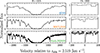 |
Fig. 2. Example of one of the absorption line systems studied in this work observed with increasingly higher resolution instruments. Each row shows the H I Lyα absorption and the region of spectrum where the strongest O I metal line should appear. The first row shows the archival SDSS data analyzed by Parks et al. (2018). The middle row shows the data taken in 2019 with WHT/ISIS. The final row shows the data taken with the high resolution echelle spectrograph Keck/HIRES. |
An exceptional property shared across all absorbers discovered through this program is the simple kinematic structures of the gas clouds. Out of the four literature EMP DLAs analyzed in Section 4.1, only one can be modeled with one gaseous component10. In contrast to this, all of these newly discovered systems (presented in Section 4.2) are accurately modeled with one gaseous component. In three-out-of-four cases, the turbulent broadening is found to be b < 5 km s−1. The relatively quiescent nature of these metal-poor absorbers is consistent with the relationship between metallicity and turbulent broadening that has been observed across the VMP DLA population (Cooke et al. 2015), and indeed may be expected given the potential mass–metallicity relation associated with the DLA host galaxies (Neeleman et al. 2013; Krogager et al. 2017). In one case, the gas cloud can be entirely well-modeled via its thermal motions. It has recently been shown that this is an ideal environment to study isotopic abundances (Welsh et al. 2020). Indeed, while these absorbers are in the sub-DLA regime, the remarkably simple kinematic structures suggest that ionization corrections are likely to be negligible.
5. Chemical abundances
In this section, we present the chemical abundance patterns of near-pristine gas clouds at cosmic noon. The metal abundances are compiled in Table 8 assuming the Asplund et al. (2021) solar abundances that are provided in Table 9. Metal abundances are calculated based on the column densities of the components that are traced by O I and Fe II. The relative column densities of the components associated with the strongest O I absorption are the least likely to suffer from the effects of ionization; the components traced by neutral gas are more likely to have all their metals associated with a single dominant ionization stage. The abundances based on just these components are therefore more reliable than measuring the relative abundances from the total column densities of the detected ions. One of the primary goals of this survey is to test if EMP DLAs (those with [Fe/H] < −3.0) exhibit an [O/Fe] abundance that is consistent with or different to VMP DLAs (those with −3.0 < [Fe/H] < −2.0).
Solar abundances adopted in this analysis from Asplund et al. (2021).
5.1. History of [O/Fe] at the lowest metallicities
The behavior of [O/Fe] at low metallicities has been the subject of many investigations in the field of chemical evolution (McWilliam 1997). It is a key indicator of the onset of enrichment from Type Ia SNe. Indeed, the behavior of [O/Fe] between −2 < [Fe/H] < −1 is well characterised for both the MW and the surrounding dwarf galaxies (e.g., Matteucci & Brocato 1990; Kirby et al. 2011; Frebel et al. 2014; Bensby et al. 2017). However, beyond [Fe/H] < −2, determining O in stars is known to be challenging. Different diagnostic lines are often shown to produce conflicting results (García Pérez et al. 2006).
The forbidden [O I] λ6300 transition is considered to be a reliable tracer of O in stars since it is known to form in local thermodynamic equilibrium (LTE) (Asplund 2005). This means the measurement of oxygen abundances using stellar spectra with these features can reach a higher degree of precision than those that require non-LTE corrections. Though, we note that the impact of 3D effects cannot be neglected and the associated correction must still be applied (Nissen et al. 2002; Collet et al. 2007; Amarsi et al. 2019). Critically, this forbidden feature is intrinsically weak and becomes challenging to detect at low metallicities. Thus, one requires high quality data in terms of both S/N and resolution to adequately detect this transition. Indeed, the reliable oxygen features in gas reservoirs suffer the opposite problem. Redwards of the Lyα forest there is the strong O Iλ1302 feature. Given the large oscillator strength, this feature is often saturated when observing gas with H I column densities approaching that of DLAs. This is naturally overcome when studying the lowest metallicity DLAs as the resulting absorption features of these systems are typically unsaturated. As a result, EMP DLAs are possibly the best environments to precisely and accurately assess the behavior of [O/Fe] at the lowest metallicities. For an EMP DLA with [Fe/H] = −3.0 and [O/Fe] = +0.40, the corresponding column density of O I would be log10N(O I)/cm−2 = 14.4. For a strong line like O Iλ1302, there is still a risk of saturation depending on the associated kinematics. In these cases, detecting unblended O Iλ1039 absorption would be invaluable. However, these systems are exceptionally rare and so it is challenging to determine the overall trends in the data.
Past work has provided information on the behavior of [O/Fe] in the VMP regime (Cooke et al. 2011). This work indicated that both VMP DLAs and VMP stars exhibit a similar distribution of [O/Fe] abundances and could be accurately modeled with a typical [O/Fe] abundance of [⟨O/Fe⟩]≃ + 0.40. At the time, there was tentative evidence that this abundance ratio would increase within the EMP regime. Our latest data provide a marked improvement in both the quality and quantity of data available for the most metal-poor DLAs.
5.2. The behavior of [O/Fe] at cosmic noon
We have completed our investigation of the [O/Fe] abundance of known EMP DLAs. In all cases we have improved the precision of the [O/Fe] abundance determinations by at least a factor of 3 or, in the case of J0903+2628, improved the upper limit by ∼1 dex. These improved measures are combined with our sample of [O/Fe] abundances of the newly discovered absorbers. We now use these data to reassess the behavior of [O/Fe] at the lowest metallicities.
Figure 3 shows the [O/Fe] abundance ratios as a function of the Fe-metallicity updated to include the DLAs analyzed and presented in this work (orange symbols), together with our Welsh et al. (2022) literature compilation of VMP and EMP DLAs (blue symbols), and MW halo stars (gray symbols; Nissen et al. 2002; Cayrel et al. 2004; García Pérez et al. 2006). In this plot, we only consider systems that have an H I column density in excess of log10N(H I)/cm−2 > 20.0. Note that the [O/Fe] abundances of these MW halo stars shown in this plot have been calculated using the [O I] 6300 Å absorption feature. They have further been corrected for 3D effects as discussed in Cooke et al. (2011).
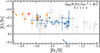 |
Fig. 3. [O/Fe] vs. [Fe/H] of DLAs and sub-DLAs. Blue data are from the literature compilation in Welsh et al. (2022) and the red points are the data presented in that work. The orange points are the DLAs presented in this work combined with the results of Welsh et al. (2023). The arrows represent systems with Fe II column densities known as upper limits. Note that we do not plot the abundances of J2150+0331 in this figure since the column density of neutral hydrogen does not meet the criteria of log10N(H I)/cm−2 > 20.0 (within the associated errors). The abundances of metal-poor stars are shown as gray symbols. |
Overall, the full sample of metal-poor absorbers provide increased statistics to assess the behavior of [O/Fe] as a function of Fe-metallicity. There are just three measurements of [O/Fe] in stars when [Fe/H] < −3.0 compared to the six DLAs reported here. This highlights the important role of new [O/Fe] measurements in this metallicity regime.
We also consider the Fe-evolution of [C/Fe] and [Si/Fe]. Figure 4 shows the [C/Fe] and [Si/Fe] abundance ratios as a function of their Fe-metallicity.
5.3. Intrinsic scatter
To quantify the behavior seen in Figures 3 and 4, we investigate the intrinsic scatter present in the data across the VMP and EMP regime. First, we categorise these absorbers based on the Fe-metallicity. We then assume that the observed abundance ratios in each regime can be well-modeled with a Gaussian centerd at a given [X/Fe] value ([X/Fe]cen) and an associated intrinsic scatter σint, [X/Fe]. The total dispersion of the sample is therefore given by the measurement error and the intrinsic scatter added in quadrature. Abundance ratios that are only known as either upper or lower limits are excluded from consideration. To find the best-fitting model given these VMP and EMP data, we run a Markov chain Monte Carlo (MCMC) likelihood analysis using the EMCEE software package (Foreman-Mackey et al. 2013). Figure 5 shows the resulting posterior distributions of the investigated parameters for [C/Fe], [O/Fe], and [Si/Fe]. In all cases, these results highlight the elevated [X/Fe] ratios observed in the EMP regime compared to the VMP regime.
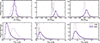 |
Fig. 5. Results of the MCMC analysis investigating the intrinsic scatter in the observed data across the VMP (pink) and EMP (purple) regime. The top row shows the posterior distributions of the central [X/Fe] values in order of their atomic number (C, O, and Si). The bottom row shows the associated distributions of the intrinsic scatter. In the middle column we show in gray the same analysis of the intrinsic scatter associated with the VMP stellar data included in Figure 3. |
For C, we find [C/Fe]cen = +0.02 ± 0.07 and ![Mathematical equation: $ \sigma_{\mathrm{int ,\, [C/Fe]}} = 0.31_{-0.05}^{+0.07} $](/articles/aa/full_html/2024/11/aa51147-24/aa51147-24-eq4.gif) for VMP DLAs. Here, and subsequently, we report the median value of the distributions while the errors are given by the associated interquartile range. Comparatively, the [C/Fe] abundance ratio of EMP DLAs can modeled with [C/Fe]cen = +0.11 ± 0.04 and
for VMP DLAs. Here, and subsequently, we report the median value of the distributions while the errors are given by the associated interquartile range. Comparatively, the [C/Fe] abundance ratio of EMP DLAs can modeled with [C/Fe]cen = +0.11 ± 0.04 and ![Mathematical equation: $ \sigma_{\mathrm{int ,\, [C/Fe]}} = 0.14_{-0.04}^{+0.06} $](/articles/aa/full_html/2024/11/aa51147-24/aa51147-24-eq5.gif) . Interestingly, the intrinsic scatter of the EMP [C/Fe] ratios is comparatively less than that observed for the VMP data. This could, in part, be due to the quality of the data available for C in the VMP regime. C is typically measured using the strong C IIλ1334 line. When available the C IIλ1036 line can also be used but it is often blended with features in the Lyα forest. At these high H I column densities the accessible C II features easily become saturated.
. Interestingly, the intrinsic scatter of the EMP [C/Fe] ratios is comparatively less than that observed for the VMP data. This could, in part, be due to the quality of the data available for C in the VMP regime. C is typically measured using the strong C IIλ1334 line. When available the C IIλ1036 line can also be used but it is often blended with features in the Lyα forest. At these high H I column densities the accessible C II features easily become saturated.
For O, we find [O/Fe]cen = +0.40 ± 0.02 and σint, [O/Fe] = 0.06 ± 0.02 for VMP DLAs. The O abundance of EMP DLAs can modeled with [O/Fe]cen = +0.50 ± 0.04 and ![Mathematical equation: $ \sigma_{\mathrm{int ,\, [O/Fe]}} = 0.13_{-0.04}^{+0.06} $](/articles/aa/full_html/2024/11/aa51147-24/aa51147-24-eq6.gif) . Both the central value and associated intrinsic scatter are found to be distinct across these metallicity regimes. This increased intrinsic scatter in the distribution of the [O/Fe] abundance ratios in the EMP regime compared to the VMP regime is reminiscent of the behavior predicted in Welsh et al. (2019, their Fig. 2) of an increased dispersion across the abundance ratios caused by a lower number of enriching stars. The ability to investigate the intrinsic scatter is dependent on both the size of the sample and the relative precision of the abundance ratios. Despite the small size of the EMP DLA sample, given the errors associated with the intrinsic scatter determinations, these data appear sufficient to produce similarly competitive constraints when compared to intrinsic scatter found using the larger sample of VMP DLAs. For reference we also investigate the intrinsic scatter associated with the VMP stellar [O/Fe] data shown in Figure 3. Interestingly, we find that, unlike the VMP DLAs, the intrinsic scatter in these data are consistent with minimal excess dispersion – [O/Fe]cen = +0.31 ± 0.01 and σint , [O/Fe] = 0.04 ± 0.02. At present, it is unclear if the excess dispersion seen in VMP DLAs is due to underestimated errors, or if DLAs exhibit a real intrinsic dispersion relative to stars of a comparable metallicity. The latter possibility could indicate that VMP DLAs are not as well-mixed as the birth sites of VMP stars. Furthermore, the VMP DLA data represent the abundances of different structures (e.g., galaxies). These different galaxies may have experienced different star formation histories, perhaps leading naturally to a higher degree of scatter in the [O/Fe] ratio in DLAs compared to that of MW halo stars. A bespoke program tailored to understanding the precise chemistry of VMP DLAs would address this possibility.
. Both the central value and associated intrinsic scatter are found to be distinct across these metallicity regimes. This increased intrinsic scatter in the distribution of the [O/Fe] abundance ratios in the EMP regime compared to the VMP regime is reminiscent of the behavior predicted in Welsh et al. (2019, their Fig. 2) of an increased dispersion across the abundance ratios caused by a lower number of enriching stars. The ability to investigate the intrinsic scatter is dependent on both the size of the sample and the relative precision of the abundance ratios. Despite the small size of the EMP DLA sample, given the errors associated with the intrinsic scatter determinations, these data appear sufficient to produce similarly competitive constraints when compared to intrinsic scatter found using the larger sample of VMP DLAs. For reference we also investigate the intrinsic scatter associated with the VMP stellar [O/Fe] data shown in Figure 3. Interestingly, we find that, unlike the VMP DLAs, the intrinsic scatter in these data are consistent with minimal excess dispersion – [O/Fe]cen = +0.31 ± 0.01 and σint , [O/Fe] = 0.04 ± 0.02. At present, it is unclear if the excess dispersion seen in VMP DLAs is due to underestimated errors, or if DLAs exhibit a real intrinsic dispersion relative to stars of a comparable metallicity. The latter possibility could indicate that VMP DLAs are not as well-mixed as the birth sites of VMP stars. Furthermore, the VMP DLA data represent the abundances of different structures (e.g., galaxies). These different galaxies may have experienced different star formation histories, perhaps leading naturally to a higher degree of scatter in the [O/Fe] ratio in DLAs compared to that of MW halo stars. A bespoke program tailored to understanding the precise chemistry of VMP DLAs would address this possibility.
The behavior of [Si/Fe] is similar to that of [O/Fe]. For Si, we find [Si/Fe]cen = +0.24 ± 0.02 and σint, [Si/Fe] = 0.14 ± 0.03 for VMP DLAs. Comparatively, the Si abundance of EMP DLAs can modeled with [Si/Fe]cen = +0.35 ± 0.06 and ![Mathematical equation: $ \sigma_{\mathrm{int ,\, [Si/Fe]}} = 0.19_{-0.05}^{+0.08} $](/articles/aa/full_html/2024/11/aa51147-24/aa51147-24-eq7.gif) . In this case, the intrinsic scatter of [Si/Fe] seems to peak at a similar position across both the VMP and EMP regime. However, as is the case for [O/Fe], the tail of the scatter extends to larger values for the EMP data.
. In this case, the intrinsic scatter of [Si/Fe] seems to peak at a similar position across both the VMP and EMP regime. However, as is the case for [O/Fe], the tail of the scatter extends to larger values for the EMP data.
Finally, we note that the [O/Fe]cen and σint, [O/Fe] values found via this analysis for both the VMP and EMP sample are consistent with our previous results (Cooke et al. 2011; Welsh et al. 2022).
6. Abundance corrections
Neutral gas reservoirs are some of the best astrophysical environments to determine the chemical abundance patterns of the most abundant chemical elements at high precision. However, there are a number of physical processes that must be considered when calculating the metal abundances from the measured gas-phase column densities. The two main physical processes that can impact abundance determinations are ionization effects and dust depletion.
6.1. Ionization corrections
Given the column densities of neutral hydrogen recorded for some of the newly discovered gas clouds in our sample, they are more appropriately described as sub-DLAs rather than bonafide DLAs. Gas clouds with an H I column density less than the DLA threshold may not be able to self-shield as effectively as DLAs. Thus, we may need to apply some ionization corrections to the observed ion column densities to uncover the intrinsic metal abundances. To minimise the impact of ionization effects, we have solely considered the relative abundances of the components traced by neutral oxygen. This restricts our analysis to the predominantly neutral gas. Moreover, we find no evidence for a statistically significant correlation between the relative ion column densities and the H I column density across our sample. This suggests that the sample sub-DLAs are not empirically different to the bonafide DLAs.
We can further test the appropriateness of this choice using the ion column densities of elements that have been detected in multiple ionization states. In the case of J1147+5034, we have information on the N(Si II)/N(Si III) ratio. The abundances of successive ions of an element can be used, alongside photoionization models, to estimate the ionization correction. We then assume that this ionization correction is appropriate for the other sub-DLAs in our sample. We define this small correction to be the difference between the true intrinsic abundance and the measured abundance based on the column densities of the dominant ionization stages:
![Mathematical equation: $$ \begin{aligned} \mathrm{[X/H] = [X_{N}/H\,i\mathrm ] + IC(X)} \end{aligned} $$](/articles/aa/full_html/2024/11/aa51147-24/aa51147-24-eq8.gif) (1)
(1)
for each observed element, X. To estimate the magnitude of such corrections, we used the CLOUDY photoionization software developed by Ferland et al. (1998, 2017) to model the newly discovered EMP DLA toward J1147+5034. We model the DLA as a plane-parallel slab of constant volume density gas in the range  , irradiated by the UV background as described in Haardt & Madau (2012) at zabs = 2.588. At this epoch, the latest determination of the UVB from Khaire & Srianand (2019) is consistent with that of Haardt & Madau (2012). Using the solar abundance scale in Asplund et al. (2021), we then scaled the metal abundances to that of the DLA ([Fe/H] = −3.13 ± 0.06). The simulations were stopped once the H I column density of the DLA was reached, at which point we output the ion column densities of the slab. As will be discussed in Section 6.2, we assume that the impact of dust at these metallicities is negligible and is therefore not included in the model. Given the assumed background radiation field, the ionization correction of each element depends on the volume density of the gas. The resulting ionization corrections calculated as a function of the gas volume density are show in the left-hand panel of Figure 6 while the associated ion ratio of the stages of Si are shown in the right-hand panel of Figure 6. These results are consistent with the alternative approach of scaling the abundances to that of a typical VMP DLA (from Cooke et al. 2011). Based on these calculations, the gas volume density of the DLA J1147+5034 can be estimated by considering the ratio of the successive ion stages of Si. The column densities in Table 5 indicate that, for this DLA, there is 2.4 times more Si II than Si III. This implies a gas density of
  . Thus, the left-hand panel of Figure 6 indicates that the ionization corrections for all observed elements are < 0.15 dex. Indeed, the negative ionization correction associated with Fe II indicates that the intrinsic [Fe/H] abundance is lower than that measured. This would place the DLA further into the EMP regime and enhance the elevated [O/Fe] abundance observed. Interestingly, a similar trend is seen for the ionization correction associated with C II. This suggests that the intrinsic [C/H] abundance is lower than that measured. Though, the observed [C/Fe] may remain unchanged given the similar correction expected for both ions. This cannot be said for Si II. The negative ionization correction associated with Si II is larger than that associated with Fe II. This could potentially cancel out any differences observed between the [Si/Fe] of VMP and EMP DLAs (Fig. 5; top right panel). Note that irrespective of the volume density, the ionization correction expected for [O/H] is negligible.
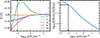 |
Fig. 6. Left: ionization corrections for the EMP DLA toward J1147+5034. We plot the expected correction for all of the observed elements as a function of gas volume density. The vertical dashed line correspond to the estimated gas density of the DLA. Right: column density ratio of successive ion stages of Si versus gas density. We also plot the observed values of the Si III/Si II ion ratio (dashed lines with gray shaded region encompassing the associated errors) and use this to determine the associated gas density. This highlights that O I is stable against ionization corrections and the impact on Fe II would only serve to increase the enhancement of [O/Fe] observed for EMP DLAs relative to VMP DLAs. |
6.2. Dust depletion
The impact of dust depletion is believed to be negligible when the iron abundance is [Fe/H] < −2 (De Cia 2018; Vladilo et al. 2018). The depletion of Si in particular is expected to be negligible for these low metallicity DLAs (Vladilo et al. 2011). Recent progress has been made toward an improved understanding about the effects of dust depletion in low metallicity environments, thanks to new measurements of dust depletion in the Large Magellanic Cloud (LMC; Roman-Duval et al. 2022) and low metallicity dwarf galaxies (Hamanowicz et al. 2024). While these studies do not reach the EMP regime studied in this paper, they do confirm that the trend of decreasing dust depletion with decreasing metallicity persists in all currently investigated environments. Indeed, if dust depletion were to be considered, it would only serve to emphasise the trend shown in Figure 3. In this scenario the VMP DLAs would in fact show lower [O/Fe] ratios and therefore the difference between the mean abundance across the VMP and EMP regimes would be increased. An empirical test of dust depletion at these metallicities would be possible if one were to obtain a measurement of ions like Mg II or Zn II; while challenging with current facilities, these measurements will become possible with the next generation of ground-based telescopes.
6.3. Redshift evolution of [C/O]
The star formation histories of low mass structures at cosmic noon are encoded in the chemistry of the most metal-poor DLAs. In Welsh et al. (2020), we presented tentative evidence of a redshift evolution of the [C/O] ratio of the most metal-poor DLAs. From chemical evolution models, one may expect to witness an increase in the [C/O] ratio at late times due to the onset of enrichment from the intermediate and low-mass stars that are bound within the same host of these gas clouds (Akerman et al. 2004; Cescutti et al. 2009; Romano et al. 2010). The low and intermediate mass stars yield a significant amount of carbon near the end of their lives, particularly the asymptotic giant branch (AGB) stars that have masses M ∼ (2 − 7) M⊙ (Karakas & Lattanzio 2007; Karakas 2010). Moreover, the carbon yields of low- and intermediate-mass stars are thought to increase with decreasing metallicity (Chiappini et al. 2003). Thus, given the metallicities of these DLAs, any associated enrichment from longer-lived stars could introduce substantial amounts of carbon. This is the case for both the (hypothetical) low-mass Pop III stars (Campbell & Lattanzio 2008) and the intermediate-mass Pop II stars (e.g., Karakas 2010).
Given the redshifts of these newly discovered systems, this sample is ideally placed to investigate the relationship between [C/O] and redshift. This sample contains both the lowest redshift EMP DLA absorber discovered to date and new data on the highest redshift EMP DLA discovered to date. We plot the [C/O] abundance ratio as a function of redshift for these latest data alongside the literature sample in Figure 7. In this case, we color the data points based on their Fe-metallicity. This figure highlights that the lowest metallicity systems (i.e., those with [Fe/H] within 0.1 dex of the EMP regime) support this trend of increasing [C/O] as redshift decreases. It is only in the most metal-poor objects that one might expect to uncover such a trend, since these systems would have experienced less ongoing star formation. Objects that have experienced ongoing star-formation are more likely to be more continuously enriched with the products of massive stars, and thus the yields of any associated AGB stars would be spread over a longer period of time. Indeed, the relatively delayed onset of enrichment from the intermediate mass stars at z ∼ 3, witnessed through the increasing [C/O] abundance at later times, may be an indication that these most metal-poor systems experience a period of quenched star-formation after the epoch of reionization.
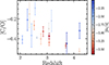 |
Fig. 7. [C/O] ratio of VMP/EMP DLAs and sub-DLAs as function of the absorption redshift. We color the systems by metallicity (see color bar). The most metal-poor systems (i.e., within 0.1 dex of the EMP regime) are indicated by the red points. These data show a trend of increasing [C/O] at lower redshifts that is not seen across the more metal rich absorbers. This indicates that these most metal-poor systems may be showcasing a unique signature of reionization quenching. This is in line with the expectation that only the most metal-poor systems would be impacted by this process at this epoch. |
7. Discussion
Our observational campaigns have yielded a high success rate of finding EMP DLAs. Of the 9 systems observed with WHT/ISIS that had sufficient final S/N, 5 of these were selected for follow-up observations with either UVES or HIRES, and 2 of them are confirmed EMP DLAs or EMP sub-DLAs (with one further candidate awaiting observations). All newly discovered absorbers have an iron abundance [Fe/H] < −2.5. This has allowed us to empirically investigate the chemical evolution of [O/Fe] across the most metal-poor systems with a larger sample size than previously available. Beyond empirical trends at cosmic noon, we can also compare our results to chemical evolution models to infer the properties of the enriching stars, and the most likely enrichment histories of near-pristine gas.
7.1. Stochastic enrichment of near-pristine DLAs
Using the observed abundance pattern of these DLAs, alongside the stochastic chemical enrichment model first described by Welsh et al. (2019), we can investigate the possible enrichment history of near-pristine gas at cosmic noon.
In this model, the mass distribution of Population III stars is modeled as a power-law: ξ(M) = k M−α, where α is the power-law slope11, and k is a multiplicative constant that is set by defining the number of stars, N⋆, that contribute to the enrichment between a minimum mass Mmin and maximum mass Mmax, given by:
 (2)
(2)
We note that Mmax represents the maximum enriching mass; stars of higher mass can form, but in our model, these stars are assumed to directly collapse to black holes and do not contribute to the enrichment (see Sukhbold et al. 2016). Since the first stars are thought to form in small multiples, this underlying mass distribution is necessarily stochastically sampled. We utilise the yields from simulations of stellar evolution to construct the expected distribution of chemical abundances given an underlying IMF model. These distributions can then be used to assess the likelihood of the observed DLA abundances given an enrichment model.
We utilise the yields from Heger & Woosley (2010) (hereafter HW10) to construct the expected distribution of chemical abundances given an underlying IMF model. The HW10 simulations model Population III progenitors with an initial metallicity Z = 0. The simulations trace nucleosynthesis processes during the lifetime of the star as well as the explosive nucleosynthesis produced by the core-collapse SNe (CCSNe). The calculated yields reported by HW10 represent the mass of each metal that is returned to the interstellar medium. These simulations explore initial progenitor masses in the range M = (10 − 100) M⊙, explosion energies from Eexp = (0.3 − 10)×1051 erg, and mixing parameters from fHe = 0 − 0.25. The explosion energy is a measure of the final kinetic energy of the ejecta at infinity, while the mixing between stellar layers is parameterised as a fraction of the helium core size. This parameter space is evaluated across 120 masses, 10 explosion energies, and 14 mixing parameters. We linearly interpolate between this grid of yields during our analysis. We refer the reader to HW10 and Welsh et al. (2019) for further details and caveats related to these yield calculations.
Our model contains six parameters: N⋆, α, Mmin, Mmax, Eexp and fHe. The range of model parameters we consider are:
In what follows, we assume that stars with masses > 10 M⊙ are physically capable of undergoing core-collapse. Therefore, we fix Mmin = 10 M⊙. Since we are only considering the yields of CCSNe, we are not sensitive to the enrichment from lower mass stars. We also assume that the mixing during the explosive burning phase of the SN can be well parameterised by a fraction of He core size. Specifically, the mixing between the stellar layers is smoothed using a boxcar filter that is 10% of the helium core size (i.e., fHe = 0.100). This is the fiducial choice from HW10 based on their comparison with the Cayrel et al. (2004) stellar sample. These empirically motivated constraints reduce the number of free parameters to 4. We apply uniform priors to all remaining model parameters. Note that the upper bound on Mmax corresponds to the mass limit above which pulsational pair-instability SNe are believed to occur (Woosley 2017).
7.2. Application to EMP DLAs
Using the [C/O], [Al/O], [Si/O], and [Fe/O] abundance ratios of the EMP DLAs in this sample, we run a MCMC maximum likelihood analysis, again using the EMCEE software package, to find the enrichment model that best fits these data. The converged chains are shown in Figure 8.
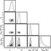 |
Fig. 8. The marginalised maximum likelihood distributions of our fiducial model parameters (main diagonal), and their associated 2D projections, given the measured chemistry of the EMP DLAs in this sample. The dark and light contours show the 68% and 95% confidence regions of these projections respectively. The EMP DLAs in this sample can be well modeled via the enrichment from a small handful of progenitors that ended their lives as low energy CCSNe. |
7.2.1. IMF slope
The slope of the IMF is found to be consistent with a Salpeter distribution; however it shows a slight preference toward a more top-heavy IMF slope. The distribution can be described by  where here, and subsequently, the reported parameter values are the median values and the interquartile range of the parameter distributions.
7.2.2. Number of enriching stars
The inferred number of enriching stars shows a preference toward low values of N⋆. The distribution is well-centerd on N⋆ = 2 ± 1 (when rounded to integer values). This is markedly lower than the number of enriching stars found for a more typical metal-poor ([Fe/H] ∼ −2.5) DLA. In Welsh et al. (2019), we found the number of enriching stars to be N⋆ < 72 (2σ) with a maximum likelihood value of N⋆ ∼ 10. These results indicate that the typical number of enriching stars decreases when considering the lowest Fe-metallicity DLAs. We have repeated the analysis of Welsh et al. (2019) after removing the known EMP DLAs and find the resulting distributions are consistent with the above scenario. The inferred N⋆ when exclusively considering VMP DLAs is higher than that found for EMP DLAs. Indeed, uniquely in the EMP regime, we are approaching a typical number of enriching stars that may be expected from one Pop. III minihalo (Skinner & Wise 2020).
7.2.3. Typical explosion energy
The distribution of the typical explosion energy is well-centerd around Eexp = (1.6 ± 0.6)×1051 erg. This is considered a moderate energy explosion for a CCSN. Indeed, this result is also in line with the carbon-enhanced absorbers that have been detected at cosmic noon (Zou et al. 2020; Saccardi et al. 2023; Salvadori et al. 2023). One way to explain this relative enhancement of [C/Fe] is via enrichment from stars with low energy explosions (Umeda & Nomoto 2003). These SNe are rich in light atomic number elements (like C) since they are more easily expelled during the explosion process.
7.2.4. Maximum enriching mass
The distribution of the maximum enriching mass is well-centerd around  . This limit was also reported by Ishigaki et al. (2018) who investigated the chemical enrichment of metal-poor halo stars. Our results tentatively support the work of Sukhbold et al. (2016), Sukhbold & Adams (2020). These authors found that, in models where the explosion is powered by a neutrino wind, only a fraction of the stars with masses above 20 M⊙ successfully launch a SN explosion. At larger masses progressively more stars collapse directly into black holes. This scenario can be tested observationally by searching for “disappearing” stars in multi-epoch imaging data (Kochanek et al. 2008; Gerke et al. 2015; Reynolds et al. 2015).
This Mmax constraint that we infer here is also consistent with the black hole masses that are being detected through gravitational waves with the Laser Interferometer Gravitational-Wave Observatory (LIGO; Abbott et al. 2016); the initial black hole masses detected through this experiment are often between M ∼ 20 − 40 M⊙. A proposed explanation of the LIGO BH masses is that they are the remnants of massive metal-poor stars. Gaia has recently detected a M ≃ 33 M⊙ black hole known as BH3 that is in a binary with a stellar companion (Gaia Collaboration 2024). This is the most massive stellar-origin black hole detected in the galaxy so far. The stellar companion of BH3 is known to be very metal-poor ([Fe/H] = −2.56 ± 0.11). Our results are in line with these observational investigations. We are finding a similar maximum mass of the enriching stellar population of some of the least polluted gas in the Universe. The lack of evidence of the chemical products of higher mass stars, may suggest that stars above this mass range are not enriching their environment and, perhaps instead, they are directly collapsing to black holes.
7.2.5. Model sensitivity
This model currently only accounts for the yields from CCSNe (not those of lower mass stars). A consequence of this is that we are only sensitive to the IMF of these relatively high mass stars and not the lower mass end of the IMF. The most sensitive tests of the low mass end of the Pop. III IMF stem from empirical observations of nearby stellar populations (Hartwig et al. 2015; Rossi et al. 2021). Furthermore, the tentative redshift evolution shown in Figure 7 may suggest that the yields of lower mass stars are influencing the [C/O] abundances of these EMP DLAs. Thus, the assumption of enrichment solely by CCSNe may not be the best choice. We reserve the inclusion of the yields of lower mass stars in the chemical evolution models for future work. For now, we rerun the analysis excluding [C/O] to mitigate the impact of potential contamination. The results of the enrichment model are stable against these changes. The slope of the IMF is less well-constrained (as is the explosion energy) but the inferences on N⋆ and Mmax are virtually unchanged.
7.2.6. Reproducing the measured abundances
Using our stochastic enrichment model, we can generate the expected abundance pattern given the inferred parameter distributions. Figure 9 shows the observed abundances of [C/O] versus [Si/O] and [Al/O] versus [Fe/O] alongside the abundance distributions expected from this model. While the observed [C/O] and [Si/O] abundances are well-recovered, it appears more challenging to reproduce the [Al/O] and [Fe/O] abundances of these EMP DLAs. This highlights both the importance of considering multiple relative abundances simultaneously and the sensitive nature of abundance pattern fitting. Indeed, it is worth noting that the [Al/O] abundances of the Cayrel et al. (2004) stellar sample are markedly subsolar, with typical values of [Al/O] ∼ −1.16. By construction, these stellar data are well-modeled by the fiducial HW10 yields (see Figure 12 of HW10). Thus, it may be impossible to reproduce the two EMP DLAs in this sample with [Al/O] abundances that are close to the solar value. Since these data are best modeled by a low number of enriching stars, we will now consider the possibility that these DLAs have been enriched by a single Population III SN.
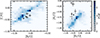 |
Fig. 9. The [C/O], [Si/O], [Al/O], and [Fe/O] abundance ratios of the systems that make up our sample (black symbols with error bars) overplotted on the joint probability distributions (blue shaded distributions) of [C/O] and [Si/O] (left) and [Al/O] and [Fe/O] (right) of the best-fit enrichment model. Overall the EMP DLA data are well-described by the inferred enrichment model. Though, there are signs that the DLAs with [Al/O] abundances close to the solar value may be challenging to reproduce. |
7.2.7. Enrichment by one Pop. III SN
Given that the inferred number of enriching stars is consistent with enrichment from a single Pop. III SN, we explore the properties of the individual stars that may have enriched each EMP DLA in our sample. For the first time, we investigate the distribution of recovered Pop. III SNe parameters across the EMP DLA population. The results of considering a single Pop III progenitor for each EMP DLA in turn are shown in Figure 10. In this scenario, we allow the degree of mixing to vary as a free parameter with a uniform prior. We show the distribution of the progenitor masses as a function of the corresponding explosion energy. The parameters and their associated errors are given by the median and interquartile range of the associated posterior distributions. Each DLA is found to be best modeled with a relatively low mass progenitor with M ≃ 18 M⊙. The explosion energies span a similar range to that found in our earlier analysis. In all cases, these EMP DLAs are best modeled by a progenitor that underwent a SN with Eexp < 3 × 1051 erg. Given the extent of the explored parameter space, the best-fit progenitor properties show minimal scatter across this sample of EMP DLAs. This may suggest that these DLAs share a relatively consistent enrichment history.
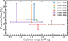 |
Fig. 10. The inferred progenitor masses as a function of their associated explosion energies from our investigation of the properties of the individual stars that can accurately model the abundances of each EMP DLA in our sample. The properties of the progenitor associated with each DLA have been found independently from one another. We represent the resulting parameter distributions by their median value and their interquartile range. These distributions are mostly non-Gaussian. In some cases, the median is close to an edge of the region bounded by the interquartile range. This is caused by a strong peak in the distribution around a particular parameter value. Compared to the full parameter space that has been explored, these DLAs show remarkably consistent progenitor properties. |
7.2.8. Pop. III versus Pop. II enrichment
At this time, our model is unable to distinguish between the enrichment between one Population III star and one Population II star with the same properties. The adopted nucleosynthetic models indicate that the yields of Pop. III and Pop. II stars are extremely similar for the abundance ratios considered in this work. The Z = 0 HW10 yields adopted are broadly consistent with the Z = 1/1000 Z⊙ yields presented in Woosley & Weaver (1995). Thus, a caveat to this analysis is that these DLAs may be equally well-modeled by two Population II stars rather than two Population III stars. Indeed, there is also the possibility of enrichment by a low number of both Pop. II and Pop. III stars. We adopt the HW10 yields given the extensive parameter space that is explored. The key result of the analysis is the low number of enriching stars that has been inferred; it is more difficult to reproduce such a low number of enriching stars with predominantly Pop. II stars. Given the low value of N⋆, we therefore consider it more likely that these environments are predominantly enriched by Pop. III stars.
7.3. DLA homogeneity?
Here we focused on the chemical abundances of a sample of neutral gas reservoirs at cosmic noon. In particular, we have looked at the intrinsic scatter present in the current data. To confidently determine the source of this scatter, one must also be confident that the sample is composed of the same class of objects.
When restricted to single sightline investigations, this can be challenging to discern. The hosts of DLAs may be a “mixed bag” of galaxies with different morphologies and associations; from protoclusters to the circumgalactic medium (CGM) (Pettini et al. 1990; Haehnelt et al. 1998; Pontzen et al. 2008; Rahmati & Schaye 2014). Indeed, recent simulations have highlighted that spatially distinct gas can appear as a single DLA or metal component when observed using a single sightline (Mandelker et al. 2021; Marra et al. 2024). Within this framework, it is interesting to consider whether there is an inherent difference between the kinematically simple gas clouds that have been discovered here compared to the more complex structures typically observed. The environments of these absorbers may also provide insight into the origins of the kinematics of the observed gas clouds (Mackenzie et al. 2019; Lofthouse et al. 2023).
Simulations of the most metal-poor DLAs suggest that they may be the descendants of halos with virial masses of  (Salvadori & Ferrara 2012). Over the course of their evolution, they are associated with low star formation rates (Yuan & Cen 2016). Indeed, it has been suggested that the most metal-poor DLAs found at z ∼ 3 may represent gas that has gone on to form the stars that are observed within the local UFD galaxy population (Webster et al. 2015). This has further been supported with chemical evolution models that infer the physical properties of these most metal poor DLAs (e.g., the associated volume density, neutral gas fraction, stellar and gaseous mass content; Cooke et al. 2015; Welsh et al. 2019). These properties have been found to be consistent with the equivalent properties within UFDs (Martin et al. 2008). Though, there are also alternative simulations that disfavor this scenario (e.g., Jeon et al. 2019). A future avenue of investigation could be to investigate whether this discrepancy can be resolved when accounting for the small scale kinematic structures of these most metal-poor DLAs (both observationally and within cosmological simulations).
8. Conclusions
We present new data of eight near-pristine absorption line systems discovered at cosmic noon and use these data to investigate early chemical enrichment. This sample includes all currently known EMP DLAs and marks the first analysis of 4 new metal-poor systems. We pay particular attention to the behavior of [O/Fe] in the EMP regime. Our main conclusions are as follows:
-
We have presented new data of the previously known EMP DLAs J0140−0838 and J1358+0349 (Figures 1 and B.1). These new data improved the precision of the [Fe/H] and [O/Fe] determinations by a factor of 3. In both cases, the latest abundances confirm that these are two of the most Fe-poor DLAs discovered to date. The [O/Fe] abundances are moderately elevated and consistent with the [O/Fe] abundances indicated by previous determinations. The improved precision is thanks to our broader wavelength coverage that includes multiple Fe II transitions covering a range of oscillator strengths.
-
We report the discovery of two new VMP DLAs and two new EMP DLAs (Figures B.2–B.5). With these data, combined with our recent analysis of the most metal-poor DLA currently known (Welsh et al. 2023), our survey has doubled the number of known EMP systems.
-
With these new statistics we re-evaluate the behavior of [O/Fe] as a function of the Fe-metallicity (Section 5 and Figure 3). We find further evidence of enhanced scatter of the [O/Fe] abundances at the lowest metallicities (Figure 5). The distinction between the typical [O/Fe] of EMP DLAs compared to VMP DLAs is less severe than previously indicated. We quantify these results using the intrinsic scatter of [O/Fe] for VMP and EMP DLAs. We find that EMP DLAs are well-modeled with [O/Fe]cen = +0.50 ± 0.04 and an intrinsic scatter of
![Mathematical equation: $ \sigma_{\mathrm{int,\, [O/Fe]}} = 0.13_{-0.04}^{+0.06} $](/articles/aa/full_html/2024/11/aa51147-24/aa51147-24-eq16.gif) . Both parameters are higher than that found for VMP DLAs, with [O/Fe]cen = +0.40 ± 0.02 and σint, [O/Fe] = 0.06 ± 0.02.
. Both parameters are higher than that found for VMP DLAs, with [O/Fe]cen = +0.40 ± 0.02 and σint, [O/Fe] = 0.06 ± 0.02. -
We exploit the detection of both Si II and Si III absorption features in the spectrum toward J1147+5034, in combination with photoionization models, to investigate the potential need for ionization corrections (Section 6.1). We find that in all cases the potential corrections are < 0.15 dex (Figure 6). These corrections could only serve to further increase the [O/Fe] values of the EMP DLAs discovered with this program.
-
We also present an updated analysis of the evolution of [C/O] as a function of redshift (Figure 7). We find that the most metal-poor systems (i.e., those within 0.1 dex of the EMP regime) show a gradually increasing [C/O] ratio at lower redshifts. This may be a sign of the onset of enrichment from the first low and intermediate mass stars associated with these gas clouds.
-
We employ a stochastic chemical enrichment model to investigate the potential enrichment histories of these EMP gas clouds (Section 7.1). We find that the [C/O], [Al/O], [Si/O], and [Fe/O] abundances of these DLAs are best modeled with an IMF slope that is consistent with a Salpeter distribution with a slight preference toward a more top-heavy IMF (Figures 8 and 9). The number of enriching stars is found to be N⋆ = 2 ± 1. This is consistent with the number of enriching stars that may be expected from one Pop. III minihalo (Skinner & Wise 2020). The maximum mass of the enriching stars is
 . Interestingly, this is broadly consistent with the black hole masses that have been detected through gravitational waves (Abbott et al. 2016) and is similarly in-line with the most massive stellar origin galactic black hole (BH3) that has recently been detected with Gaia alongside a metal-poor companion (Gaia Collaboration 2024). A possible explanation of the LIGO detected black holes, that is supported by the recent Gaia detection, is that they are the remnants of massive metal-poor stars in the early Universe that failed to explode as core-collapse SNe. Indeed, we are finding a similar maximum mass of the enriching stellar population of some of the least polluted gas in the Universe. The lack of evidence for the chemical products of higher mass stars may suggest that stars above this mass range are not enriching their environment and, perhaps instead, they are directly collapsing to black holes. This limit was also reported by Ishigaki et al. (2018) who investigated the chemical enrichment of metal-poor halo stars.
 -
We propose that an interesting avenue of future investigation is whether there is an intrinsic difference between kinematically simple EMP DLAs compared to those with more complex structures (Section 7.3). Indeed, this could be an avenue to discern the range of potential hosts of these most metal-poor gas reservoirs (Salvadori & Ferrara 2012; Webster et al. 2015; Jeon et al. 2019; Mandelker et al. 2021).
This survey has enabled the first detailed understanding of EMP DLAs, and the potential of these gas clouds to study the properties of the first stars. Upcoming surveys (e.g., DESI, WEAVE, and 4MOST Dalton et al. 2012; de Jong et al. 2012; DESI Collaboration 2016a,b, 2024; Pieri et al. 2016) will provide new EMP DLA candidates to study the chemical enrichment of near-pristine gas. If an elevated [O/Fe] abundance can be attributed to enrichment by metal-free stars, then the DLAs analyzed in this work may provide a signpost to some of the most pristine environments in the high redshift universe, and would be an ideal place to search for Population III host galaxies and perhaps even the light from Population III SNe using the James Webb Space Telescope.
The square bracket notation denotes the logarithmic number abundance ratio of elements X and H relative to their solar values X⊙ and H⊙, i.e., [X/H]=log10(NX/NH)−log10(NX/NH)⊙.
The α elements are those that can be produced via the α-capture process (e.g., O, Ne, Mg, Si, S, Ar, and Ca).
Hires REDUX is available from: https://www.ucolick.org/~xavier/HIRedux/
Pypeit is available from: https://pypeit.readthedocs.io/en/release/index.html
UVES_POPLER is available from: https://github.com/MTMurphy77/UVES_popler
The exception to this is the J1147+5034 Keck/HIRES data. These data were combined with the PypeIt coadding tool.
ALIS is available from:
We visually inspected the troughs of saturated absorption features to confirm this is the case.
We also cover the Fe IIλ2344 feature however this is blended with telluric absorption.
These four systems are those with previous high resolution data available.
In our formulation, α = 2.35 corresponds to a Salpeter IMF.
Acknowledgments
We thank the anonymous referee for their prompt and thorough review of this paper. We thank Valentina D’Odorico, Paolo Molaro, and Trystyn Berg for helpful comments and feedback. This paper is based on observations collected at the William Herschel Telescope (WHT) at the Roque de los Muchachos Observatory on the island of La Palma in the Canary Islands, Spain (program ID: W/2019B/04). L. A. W is particularly grateful to Lucia Suarez-Andres and all of the staff astronomers at the WHT who provided significant support during the observing runs throughout the months of Sep. – Dec. 2019. This paper is further based on observations collected at the European Organisation for Astronomical Research in the Southern Hemisphere, Chile, and at the W. M. Keck Observatory which is operated as a scientific partnership among the California Institute of Technology, the University of California and the National Aeronautics and Space Administration (program IDs in Table 1). The Observatory was made possible by the generous financial support of the W. M. Keck Foundation. The authors wish to recognize and acknowledge the very significant cultural role and reverence that the summit of Maunakea has always had within the indigenous Hawaiian community. We are most fortunate to have the opportunity to conduct observations from this mountain. We are also grateful to the staff astronomers at the VLT and Keck Observatory for their assistance with the observations. This work has been supported by Fondazione Cariplo, grant No 2018-2329. During this work, R. J. C. was supported by a Royal Society University Research Fellowship. We acknowledge support from STFC (ST/L00075X/1, ST/P000541/1). This project has received funding from the European Research Council (ERC) under the European Union’s Horizon 2020 research and innovation program (grant agreement No 757535). This work used the DiRAC@Durham facility managed by the Institute for Computational Cosmology on behalf of the STFC DiRAC HPC Facility (www.dirac.ac.uk). The equipment was funded by BEIS capital funding via STFC capital grants ST/P002293/1, ST/R002371/1 and ST/S002502/1, Durham University and STFC operations grant ST/R000832/1. DiRAC is part of the National e-Infrastructure. This research has made use of NASA’s Astrophysics Data System.
References
- Abbott, B. P., Abbott, R., Abbott, T. D., et al. 2016, Phys. Rev. Lett., 116, 061102 [Google Scholar]
- Akerman, C. J., Carigi, L., Nissen, P. E., Pettini, M., & Asplund, M. 2004, A&A, 414, 931 [NASA ADS] [CrossRef] [EDP Sciences] [Google Scholar]
- Amarsi, A. M., Nissen, P. E., & Skúladóttir, Á. 2019, A&A, 630, A104 [NASA ADS] [CrossRef] [EDP Sciences] [Google Scholar]
- Aoki, W., Frebel, A., Christlieb, N., et al. 2006, ApJ, 639, 897 [Google Scholar]
- Arentsen, A., Starkenburg, E., Martin, N. F., et al. 2020, MNRAS, 491, L11 [Google Scholar]
- Asplund, M. 2005, ARA&A, 43, 481 [Google Scholar]
- Asplund, M., Amarsi, A. M., & Grevesse, N. 2021, A&A, 653, A141 [NASA ADS] [CrossRef] [EDP Sciences] [Google Scholar]
- Asplund, M., Grevesse, N., Sauval, A. J., & Scott, P. 2009, ARA&A, 47, 481 [NASA ADS] [CrossRef] [Google Scholar]
- Bañados, E., Rauch, M., Decarli, R., et al. 2019, ApJ, 885, 59 [CrossRef] [Google Scholar]
- Beers, T. C., & Christlieb, N. 2005, ARA&A, 43, 531 [NASA ADS] [CrossRef] [Google Scholar]
- Beers, T. C., Preston, G. W., & Shectman, S. A. 1985, AJ, 90, 2089 [NASA ADS] [CrossRef] [Google Scholar]
- Bensby, T., Feltzing, S., Gould, A., et al. 2017, A&A, 605, A89 [NASA ADS] [CrossRef] [EDP Sciences] [Google Scholar]
- Berg, T. A. M., Hayes, C. R., Cristiani, S., et al. 2024, MNRAS, 531, 3815 [NASA ADS] [CrossRef] [Google Scholar]
- Bernstein, R. M., Burles, S. M., & Prochaska, J. X. 2015, PASP, 127, 911 [NASA ADS] [CrossRef] [Google Scholar]
- Bond, H. E. 1980, ApJS, 44, 517 [NASA ADS] [CrossRef] [Google Scholar]
- Bromm, V., & Yoshida, N. 2011, ARA&A, 49, 373 [CrossRef] [Google Scholar]
- Campbell, S. W., & Lattanzio, J. C. 2008, A&A, 490, 769 [NASA ADS] [CrossRef] [EDP Sciences] [Google Scholar]
- Cayrel, R., Depagne, E., Spite, M., et al. 2004, A&A, 416, 1117 [NASA ADS] [CrossRef] [EDP Sciences] [Google Scholar]
- Centurión, M., Molaro, P., Vladilo, G., et al. 2003, A&A, 403, 55 [NASA ADS] [CrossRef] [EDP Sciences] [Google Scholar]
- Cescutti, G., Matteucci, F., McWilliam, A., & Chiappini, C. 2009, A&A, 505, 605 [NASA ADS] [CrossRef] [EDP Sciences] [Google Scholar]
- Chiappini, C., Romano, D., & Matteucci, F. 2003, MNRAS, 339, 63 [NASA ADS] [CrossRef] [Google Scholar]
- Collet, R., Asplund, M., & Trampedach, R. 2007, A&A, 469, 687 [NASA ADS] [CrossRef] [EDP Sciences] [Google Scholar]
- Cooke, R., Pettini, M., Steidel, C. C., Rudie, G. C., & Nissen, P. E. 2011, MNRAS, 417, 1534 [CrossRef] [Google Scholar]
- Cooke, R. J., Pettini, M., Jorgenson, R. A., Murphy, M. T., & Steidel, C. C. 2014, ApJ, 781, 31 [NASA ADS] [CrossRef] [Google Scholar]
- Cooke, R. J., Pettini, M., & Jorgenson, R. A. 2015, ApJ, 800, 12 [NASA ADS] [CrossRef] [Google Scholar]
- Cooke, R. J., Pettini, M., Nollett, K. M., & Jorgenson, R. 2016, ApJ, 830, 148 [Google Scholar]
- Cooke, R. J., Pettini, M., & Steidel, C. C. 2017, MNRAS, 467, 802 [NASA ADS] [Google Scholar]
- Dalton, G., Trager, S. C., Abrams, D. C., et al. 2012, SPIE Conf. Ser., 8446, 84460P [Google Scholar]
- De Cia, A. 2018, A&A, 613, L2 [NASA ADS] [CrossRef] [EDP Sciences] [Google Scholar]
- de Jong, R. S., Bellido-Tirado, O., Chiappini, C., et al. 2012, SPIE Conf. Ser., 8446, 84460T [Google Scholar]
- Dekker, H., D’Odorico, S., Kaufer, A., Delabre, B., & Kotzlowski, H. 2000, Proc. SPIE, 4008, 534 [Google Scholar]
- DESI Collaboration (Aghamousa, A., et al.) 2016a, ArXiv e-prints [arXiv:1611.00036] [Google Scholar]
- DESI Collaboration (Aghamousa, A., et al.) 2016b, ArXiv e-prints [arXiv:1611.00037] [Google Scholar]
- DESI Collaboration (Adame, A. G., et al.) 2024, AJ, 168, 58 [NASA ADS] [CrossRef] [Google Scholar]
- Dessauges-Zavadsky, M., D’Odorico, S., McMahon, R. G., et al. 2001, A&A, 370, 426 [NASA ADS] [CrossRef] [EDP Sciences] [Google Scholar]
- D’Odorico, V., Bolton, J. S., Christensen, L., et al. 2023, Exp. Astron., submitted [arXiv:2311.16803] [Google Scholar]
- Dutta, R., Srianand, R., Rahmani, H., et al. 2014, MNRAS, 440, 307 [NASA ADS] [CrossRef] [Google Scholar]
- Edvardsson, B., Andersen, J., Gustafsson, B., et al. 1993, A&A, 275, 101 [NASA ADS] [Google Scholar]
- Ellison, S. L., Prochaska, J. X., Hennawi, J., et al. 2010, MNRAS, 406, 1435 [NASA ADS] [Google Scholar]
- Erni, P., Richter, P., Ledoux, C., & Petitjean, P. 2006, A&A, 451, 19 [NASA ADS] [CrossRef] [EDP Sciences] [Google Scholar]
- Ferland, G. J., Korista, K. T., Verner, D. A., et al. 1998, PASP, 110, 761 [Google Scholar]
- Ferland, G. J., Chatzikos, M., Guzmán, F., et al. 2017, Rev. Mex. Astron. Astrofis., 53, 385 [NASA ADS] [Google Scholar]
- Foreman-Mackey, D., Hogg, D. W., Lang, D., & Goodman, J. 2013, PASP, 125, 306 [Google Scholar]
- Frebel, A., & Norris, J. E. 2015, ARA&A, 53, 631 [NASA ADS] [CrossRef] [Google Scholar]
- Frebel, A., Aoki, W., Christlieb, N., et al. 2005, Nature, 434, 871 [CrossRef] [Google Scholar]
- Frebel, A., Simon, J. D., & Kirby, E. N. 2014, ApJ, 786, 74 [NASA ADS] [CrossRef] [Google Scholar]
- Fumagalli, M., O’Meara, J. M., & Prochaska, J. X. 2011, Science, 334, 1245 [NASA ADS] [CrossRef] [Google Scholar]
- Gaia Collaboration (Panuzzo, P., et al.) 2024, A&A, 686, L2 [NASA ADS] [CrossRef] [EDP Sciences] [Google Scholar]
- García Pérez, A. E., Asplund, M., Primas, F., Nissen, P. E., & Gustafsson, B. 2006, A&A, 451, 621 [NASA ADS] [CrossRef] [EDP Sciences] [Google Scholar]
- Gerke, J. R., Kochanek, C. S., & Stanek, K. Z. 2015, MNRAS, 450, 3289 [Google Scholar]
- Haardt, F., & Madau, P. 2012, ApJ, 746, 125 [Google Scholar]
- Haehnelt, M. G., Steinmetz, M., & Rauch, M. 1998, ApJ, 495, 647 [NASA ADS] [CrossRef] [Google Scholar]
- Hamanowicz, A., Tchernyshyov, K., Roman-Duval, J., et al. 2024, ApJ, 966, 80 [NASA ADS] [CrossRef] [Google Scholar]
- Hartwig, T., Bromm, V., Klessen, R. S., & Glover, S. C. O. 2015, MNRAS, 447, 3892 [NASA ADS] [CrossRef] [Google Scholar]
- Hartwig, T., Yoshida, N., Magg, M., et al. 2018, MNRAS, 478, 1795 [CrossRef] [Google Scholar]
- Hartwig, T., Ishigaki, M. N., Kobayashi, C., Tominaga, N., & Nomoto, K. 2023, ApJ, 946, 20 [NASA ADS] [CrossRef] [Google Scholar]
- Heger, A., & Woosley, S. E. 2010, ApJ, 724, 341 [Google Scholar]
- Hendricks, B., Koch, A., Lanfranchi, G. A., et al. 2014, ApJ, 785, 102 [NASA ADS] [CrossRef] [Google Scholar]
- Hill, V., Skúladóttir, Á., Tolstoy, E., et al. 2019, A&A, 626, A15 [NASA ADS] [CrossRef] [EDP Sciences] [Google Scholar]
- Ishigaki, M. N., Chiba, M., & Aoki, W. 2012, ApJ, 753, 64 [NASA ADS] [CrossRef] [Google Scholar]
- Ishigaki, M. N., Tominaga, N., Kobayashi, C., & Nomoto, K. 2018, ApJ, 857, 46 [Google Scholar]
- Jeon, M., Besla, G., & Bromm, V. 2019, ApJ, 878, 98 [CrossRef] [Google Scholar]
- Karakas, A. I. 2010, MNRAS, 403, 1413 [NASA ADS] [CrossRef] [Google Scholar]
- Karakas, A., & Lattanzio, J. C. 2007, PASA, 24, 103 [NASA ADS] [CrossRef] [Google Scholar]
- Khaire, V., & Srianand, R. 2019, MNRAS, 484, 4174 [NASA ADS] [CrossRef] [Google Scholar]
- Kirby, E. N., Cohen, J. G., Smith, G. H., et al. 2011, ApJ, 727, 79 [NASA ADS] [CrossRef] [Google Scholar]
- Kirihara, T., Hasegawa, K., Umemura, M., Mori, M., & Ishiyama, T. 2020, MNRAS, 491, 4387 [NASA ADS] [CrossRef] [Google Scholar]
- Klessen, R. S., & Glover, S. C. O. 2023, ARA&A, 61, 65 [NASA ADS] [CrossRef] [Google Scholar]
- Kobayashi, C., Karakas, A. I., & Lugaro, M. 2020, ApJ, 900, 179 [Google Scholar]
- Kochanek, C. S., Beacom, J. F., Kistler, M. D., et al. 2008, ApJ, 684, 1336 [NASA ADS] [CrossRef] [Google Scholar]
- Krogager, J. K., Møller, P., Fynbo, J. P. U., & Noterdaeme, P. 2017, MNRAS, 469, 2959 [NASA ADS] [CrossRef] [Google Scholar]
- Lehner, N., Kopenhafer, C., O’Meara, J. M., et al. 2022, ApJ, 936, 156 [NASA ADS] [CrossRef] [Google Scholar]
- Lodders, K. 2019, ArXiv e-prints [arXiv:1912.00844] [Google Scholar]
- Lofthouse, E. K., Fumagalli, M., Fossati, M., et al. 2023, MNRAS, 518, 305 [Google Scholar]
- Mackenzie, R., Fumagalli, M., Theuns, T., et al. 2019, MNRAS, 487, 5070 [NASA ADS] [CrossRef] [Google Scholar]
- Magg, E., Bergemann, M., Serenelli, A., et al. 2022, A&A, 661, A140 [NASA ADS] [CrossRef] [EDP Sciences] [Google Scholar]
- Maio, U., & Tescari, E. 2015, MNRAS, 453, 3798 [Google Scholar]
- Mandelker, N., van den Bosch, F. C., Springel, V., et al. 2021, ApJ, 923, 115 [NASA ADS] [CrossRef] [Google Scholar]
- Marra, R., Churchill, C. W., Kacprzak, G. G., et al. 2024, MNRAS, 527, 10522 [Google Scholar]
- Martin, N. F., de Jong, J. T. A., & Rix, H.-W. 2008, ApJ, 684, 1075 [NASA ADS] [CrossRef] [Google Scholar]
- Matteucci, F. 2003, Ap&SS, 284, 539 [CrossRef] [Google Scholar]
- Matteucci, F., & Brocato, E. 1990, ApJ, 365, 539 [CrossRef] [Google Scholar]
- McWilliam, A. 1997, ARA&A, 35, 503 [NASA ADS] [CrossRef] [Google Scholar]
- Molaro, P., Bonifacio, P., Centurión, M., et al. 2000, ApJ, 541, 54 [NASA ADS] [CrossRef] [Google Scholar]
- Morrison, S., Kulkarni, V. P., Som, D., et al. 2016, ApJ, 830, 158 [NASA ADS] [CrossRef] [Google Scholar]
- Murphy, M. T., Kacprzak, G. G., Savorgnan, G. A. D., & Carswell, R. F. 2019, MNRAS, 482, 3458 [NASA ADS] [CrossRef] [Google Scholar]
- Neeleman, M., Wolfe, A. M., Prochaska, J. X., & Rafelski, M. 2013, ApJ, 769, 54 [NASA ADS] [CrossRef] [Google Scholar]
- Nissen, P. E., Primas, F., Asplund, M., & Lambert, D. L. 2002, A&A, 390, 235 [NASA ADS] [CrossRef] [EDP Sciences] [Google Scholar]
- Noterdaeme, P., Balashev, S., Ledoux, C., et al. 2021, A&A, 651, A78 [NASA ADS] [CrossRef] [EDP Sciences] [Google Scholar]
- Nuñez, E. H., Kirby, E. N., & Steidel, C. C. 2022, ApJ, 927, 64 [CrossRef] [Google Scholar]
- O’Meara, J. M., Tytler, D., Kirkman, D., et al. 2001, ApJ, 552, 718 [CrossRef] [Google Scholar]
- Parks, D., Prochaska, J. X., Dong, S., & Cai, Z. 2018, MNRAS, 476, 1151 [NASA ADS] [CrossRef] [Google Scholar]
- Penprase, B. E., Prochaska, J. X., Sargent, W. L. W., Toro-Martinez, I., & Beeler, D. J. 2010, ApJ, 721, 1 [NASA ADS] [CrossRef] [Google Scholar]
- Péroux, C., & Howk, J. C. 2020, ARA&A, 58, 363 [CrossRef] [Google Scholar]
- Petitjean, P., Ledoux, C., & Srianand, R. 2008, A&A, 480, 349 [NASA ADS] [CrossRef] [EDP Sciences] [Google Scholar]
- Pettini, M., Boksenberg, A., & Hunstead, R. W. 1990, ApJ, 348, 48 [NASA ADS] [CrossRef] [Google Scholar]
- Pettini, M., Zych, B. J., Steidel, C. C., & Chaffee, F. H. 2008, MNRAS, 385, 2011 [NASA ADS] [CrossRef] [Google Scholar]
- Pieri, M. M., Bonoli, S., Chaves-Montero, J., et al. 2016, in SF2A-2016: Proceedings of the Annual meeting of the French Society of Astronomy and Astrophysics, eds. C. Reylé, J. Richard, L. Cambrésy, et al., 259 [Google Scholar]
- Pontzen, A., Governato, F., Pettini, M., et al. 2008, MNRAS, 390, 1349 [NASA ADS] [Google Scholar]
- Prochaska, J. X., Hennawi, J. F., & Herbert-Fort, S. 2008, ApJ, 675, 1002 [Google Scholar]
- Prochaska, J., Hennawi, J., Westfall, K., et al. 2020, J. Open Source Softw., 5, 2308 [NASA ADS] [CrossRef] [Google Scholar]
- Rafelski, M., Wolfe, A. M., Prochaska, J. X., Neeleman, M., & Mendez, A. J. 2012, ApJ, 755, 89 [NASA ADS] [CrossRef] [Google Scholar]
- Rahmati, A., & Schaye, J. 2014, MNRAS, 438, 529 [NASA ADS] [CrossRef] [Google Scholar]
- Reynolds, T. M., Fraser, M., & Gilmore, G. 2015, MNRAS, 453, 2885 [Google Scholar]
- Robert, P. F., Murphy, M. T., O’Meara, J. M., Crighton, N. H. M., & Fumagalli, M. 2019, MNRAS, 483, 2736 [NASA ADS] [CrossRef] [Google Scholar]
- Roman-Duval, J., Jenkins, E. B., Tchernyshyov, K., et al. 2022, ApJ, 935, 105 [Google Scholar]
- Romano, D., Karakas, A. I., Tosi, M., & Matteucci, F. 2010, A&A, 522, A32 [NASA ADS] [CrossRef] [EDP Sciences] [Google Scholar]
- Rossi, M., Salvadori, S., & Skúladóttir, Á. 2021, MNRAS, 503, 6026 [NASA ADS] [CrossRef] [Google Scholar]
- Saccardi, A., Salvadori, S., D’Odorico, V., et al. 2023, ApJ, 948, 35 [NASA ADS] [CrossRef] [Google Scholar]
- Salvadori, S., & Ferrara, A. 2012, MNRAS, 421, L29 [NASA ADS] [CrossRef] [Google Scholar]
- Salvadori, S., D’Odorico, V., Saccardi, A., Skúladóttir, Á., & Vanni, I. 2023, Mem. Soc. Astron. Ital., 94, 215 [NASA ADS] [Google Scholar]
- Skinner, D., & Wise, J. H. 2020, MNRAS, 492, 4386 [NASA ADS] [CrossRef] [Google Scholar]
- Sodini, A., D’Odorico, V., Salvadori, S., et al. 2024, A&A, 687, A314 [NASA ADS] [CrossRef] [EDP Sciences] [Google Scholar]
- Starkenburg, E., Hill, V., Tolstoy, E., et al. 2013, A&A, 549, A88 [NASA ADS] [CrossRef] [EDP Sciences] [Google Scholar]
- Starkenburg, E., Martin, N., Youakim, K., et al. 2017, MNRAS, 471, 2587 [NASA ADS] [CrossRef] [Google Scholar]
- Sukhbold, T., & Adams, S. 2020, MNRAS, 492, 2578 [Google Scholar]
- Sukhbold, T., Ertl, T., Woosley, S. E., Brown, J. M., & Janka, H.-T. 2016, ApJ, 821, 38 [Google Scholar]
- Tinsley, B. M. 1979, ApJ, 229, 1046 [Google Scholar]
- Tolstoy, E., Hill, V., & Tosi, M. 2009, ARA&A, 47, 371 [Google Scholar]
- Umeda, H., & Nomoto, K. 2003, Nature, 422, 871 [NASA ADS] [CrossRef] [PubMed] [Google Scholar]
- Vangioni, E., Dvorkin, I., Olive, K. A., et al. 2018, MNRAS, 477, 56 [NASA ADS] [CrossRef] [Google Scholar]
- Vanni, I., Salvadori, S., Skúladóttir, Á., Rossi, M., & Koutsouridou, I. 2023, MNRAS, 526, 2620 [NASA ADS] [CrossRef] [Google Scholar]
- Velichko, A., De Cia, A., Konstantopoulou, C., et al. 2024, A&A, 685, A103 [NASA ADS] [CrossRef] [EDP Sciences] [Google Scholar]
- Vladilo, G., Abate, C., Yin, J., Cescutti, G., & Matteucci, F. 2011, A&A, 530, A33 [NASA ADS] [CrossRef] [EDP Sciences] [Google Scholar]
- Vladilo, G., Gioannini, L., Matteucci, F., & Palla, M. 2018, ApJ, 868, 127 [NASA ADS] [CrossRef] [Google Scholar]
- Vogt, S. S., Allen, S. L., Bigelow, B. C., et al. 1994, SPIE Conf. Ser., 2198, 362 [NASA ADS] [Google Scholar]
- Webster, D., Bland-Hawthorn, J., & Sutherland, R. S. 2015, ApJ, 804, 110 [NASA ADS] [CrossRef] [Google Scholar]
- Welsh, L., Cooke, R., & Fumagalli, M. 2019, MNRAS, 487, 3363 [NASA ADS] [Google Scholar]
- Welsh, L., Cooke, R., Fumagalli, M., & Pettini, M. 2020, MNRAS, 494, 1411 [NASA ADS] [CrossRef] [Google Scholar]
- Welsh, L., Cooke, R., Fumagalli, M., & Pettini, M. 2022, ApJ, 929, 158 [NASA ADS] [CrossRef] [Google Scholar]
- Welsh, L., Cooke, R., Fumagalli, M., & Pettini, M. 2023, MNRAS, 525, 527 [NASA ADS] [CrossRef] [Google Scholar]
- Wheeler, J. C., Sneden, C., & Truran, J. W., Jr 1989, ARA&A, 27, 279 [NASA ADS] [CrossRef] [Google Scholar]
- Wolfe, A. M., Gawiser, E., & Prochaska, J. X. 2005, ARA&A, 43, 861 [NASA ADS] [CrossRef] [Google Scholar]
- Woosley, S. E. 2017, ApJ, 836, 244 [Google Scholar]
- Woosley, S. E., & Weaver, T. A. 1995, ApJS, 101, 181 [Google Scholar]
- Yuan, S., & Cen, R. 2016, MNRAS, 457, 487 [CrossRef] [Google Scholar]
- Zafar, T., Centurión, M., Péroux, C., et al. 2014, MNRAS, 444, 744 [NASA ADS] [CrossRef] [Google Scholar]
- Zou, S., Petitjean, P., Noterdaeme, P., et al. 2020, ApJ, 901, 105 [NASA ADS] [CrossRef] [Google Scholar]
Appendix A: Telluric line removal
In this appendix we show the treatment of telluric absorption removal for the spectrum of J1358+0349. Prior to combining the exposures, we first remove the telluric absorption near the Fe II features of interest using a telluric standard star. The Fe IIλ2382 line appears in two orders and we perform this correction to both orders separately. An example of the data near the Fe IIλ2382 line prior to the removal of the telluric lines is shown in Figure A.1. This figure shows the relevant wavelength region for a selection of exposures alongside the equivalent data from the observations of the telluric star.
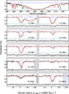 |
Fig. A.1. A subset of the UVES data taken for J1358+0349 (gray histogram) overplotted with the associated observations of the telluric standard star (blue histogram). These panels show the first four exposures of this target. The region shaded in red covers the 1.5 Å region of the spectrum centerd on where the Fe IIλ2382 feature of the central DLA component should fall. |
Appendix B: Additional figures
This appendix contains the figures showcasing the model fits to the absorption line systems observed and utilized in our analysis.
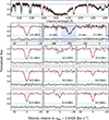 |
Fig. B.1. Same as Figure 1 for the DLA at zabs = 2.85287 toward J1358+0349. Note the different y-scale of the bottom four panels. When fitting hydrogen (top panel) we often fit a selection of unrelated narrow absorption features simultaneously. We only fit those necessary to best capture the shape of the continuum alongside the wings of the damped Lyα profile. |
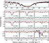 |
Fig. B.2. Same as Figure 1 for the DLA at zabs = 2.41623 toward the quasar J0239−0649. Note the x-axis of the panel showing N I is different to that showing the other ions. This is to showcase the three features of the N Iλ1200 triplet. |
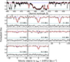 |
Fig. B.3. Same as Figure B.2 for the DLA at zabs = 2.51888 toward J1147+5034. Note the different y-axis scale of the fourth row. Note also the Si IIIλ1206 absorption feature in the top panel at ∼4246 Å. Also note that the Si IIλ1808 feature is not detected. Combined with the detection of stronger Si II lines, the coverage of this feature is useful to determine the total Si II column density. |
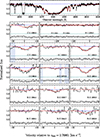 |
Fig. B.4. Same as Figure B.2 for the DLA at zabs = 2.69712 toward J2150+0331. Again, note the information provided by the non-detection of Si IIλ1808. |
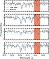 |
Fig. B.5. Same as Figure B.2 for the DLA at zabs = 2.76861 toward J2308+0854. Again, note the distinct x-axis of the panel showcasing the N I triplet and the non-detection of Si IIλ1808. |
All Tables
Ion column densities of the DLA at zabs = 3.696621 ± 0.000002 toward the quasar J0140−0839.
All Figures
|
Fig. 1. Continuum normalized UVES data (black histograms) of the absorption features associated with the DLA at zabs = 3.69662 toward J0140−0819. The best-fitting model is shown with the red curves. The blue dashed line indicates the position of the continuum while the green dashed line indicates the zero-level. The ticks above the absorption features indicate the centre of the Voigt line profiles. The features of the strongest components are distinguished via red ticks while those of weaker components are shown in blue. These strongest components are also often associated with the predominantly neutral gas. The purple ticks indicate absorption features unrelated to the DLA. Below the zero-level, we show the residuals of this fit (black histogram) where the gray shaded band encompasses the 2σ deviates between the model and the data. The vertical blue shaded bands indicate the regions of the spectrum not included in the fit. Note that the full complement of available data were used in calculating the best-fit model, while we only show a selection of the data in this figure to showcase the model and the data. We also note that the y-axis scale is different in some panels to highlight the very weak absorption lines. |
| In the text | |
|
Fig. 2. Example of one of the absorption line systems studied in this work observed with increasingly higher resolution instruments. Each row shows the H I Lyα absorption and the region of spectrum where the strongest O I metal line should appear. The first row shows the archival SDSS data analyzed by Parks et al. (2018). The middle row shows the data taken in 2019 with WHT/ISIS. The final row shows the data taken with the high resolution echelle spectrograph Keck/HIRES. |
| In the text | |
|
Fig. 3. [O/Fe] vs. [Fe/H] of DLAs and sub-DLAs. Blue data are from the literature compilation in Welsh et al. (2022) and the red points are the data presented in that work. The orange points are the DLAs presented in this work combined with the results of Welsh et al. (2023). The arrows represent systems with Fe II column densities known as upper limits. Note that we do not plot the abundances of J2150+0331 in this figure since the column density of neutral hydrogen does not meet the criteria of log10N(H I)/cm−2 > 20.0 (within the associated errors). The abundances of metal-poor stars are shown as gray symbols. |
| In the text | |
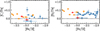 |
Fig. 4. Same as Figure 3 but the panels showcase [C/Fe] and [Si/Fe] respectively. |
| In the text | |
|
Fig. 5. Results of the MCMC analysis investigating the intrinsic scatter in the observed data across the VMP (pink) and EMP (purple) regime. The top row shows the posterior distributions of the central [X/Fe] values in order of their atomic number (C, O, and Si). The bottom row shows the associated distributions of the intrinsic scatter. In the middle column we show in gray the same analysis of the intrinsic scatter associated with the VMP stellar data included in Figure 3. |
| In the text | |
|
Fig. 6. Left: ionization corrections for the EMP DLA toward J1147+5034. We plot the expected correction for all of the observed elements as a function of gas volume density. The vertical dashed line correspond to the estimated gas density of the DLA. Right: column density ratio of successive ion stages of Si versus gas density. We also plot the observed values of the Si III/Si II ion ratio (dashed lines with gray shaded region encompassing the associated errors) and use this to determine the associated gas density. This highlights that O I is stable against ionization corrections and the impact on Fe II would only serve to increase the enhancement of [O/Fe] observed for EMP DLAs relative to VMP DLAs. |
| In the text | |
|
Fig. 7. [C/O] ratio of VMP/EMP DLAs and sub-DLAs as function of the absorption redshift. We color the systems by metallicity (see color bar). The most metal-poor systems (i.e., within 0.1 dex of the EMP regime) are indicated by the red points. These data show a trend of increasing [C/O] at lower redshifts that is not seen across the more metal rich absorbers. This indicates that these most metal-poor systems may be showcasing a unique signature of reionization quenching. This is in line with the expectation that only the most metal-poor systems would be impacted by this process at this epoch. |
| In the text | |
|
Fig. 8. The marginalised maximum likelihood distributions of our fiducial model parameters (main diagonal), and their associated 2D projections, given the measured chemistry of the EMP DLAs in this sample. The dark and light contours show the 68% and 95% confidence regions of these projections respectively. The EMP DLAs in this sample can be well modeled via the enrichment from a small handful of progenitors that ended their lives as low energy CCSNe. |
| In the text | |
|
Fig. 9. The [C/O], [Si/O], [Al/O], and [Fe/O] abundance ratios of the systems that make up our sample (black symbols with error bars) overplotted on the joint probability distributions (blue shaded distributions) of [C/O] and [Si/O] (left) and [Al/O] and [Fe/O] (right) of the best-fit enrichment model. Overall the EMP DLA data are well-described by the inferred enrichment model. Though, there are signs that the DLAs with [Al/O] abundances close to the solar value may be challenging to reproduce. |
| In the text | |
|
Fig. 10. The inferred progenitor masses as a function of their associated explosion energies from our investigation of the properties of the individual stars that can accurately model the abundances of each EMP DLA in our sample. The properties of the progenitor associated with each DLA have been found independently from one another. We represent the resulting parameter distributions by their median value and their interquartile range. These distributions are mostly non-Gaussian. In some cases, the median is close to an edge of the region bounded by the interquartile range. This is caused by a strong peak in the distribution around a particular parameter value. Compared to the full parameter space that has been explored, these DLAs show remarkably consistent progenitor properties. |
| In the text | |
|
Fig. A.1. A subset of the UVES data taken for J1358+0349 (gray histogram) overplotted with the associated observations of the telluric standard star (blue histogram). These panels show the first four exposures of this target. The region shaded in red covers the 1.5 Å region of the spectrum centerd on where the Fe IIλ2382 feature of the central DLA component should fall. |
| In the text | |
|
Fig. B.1. Same as Figure 1 for the DLA at zabs = 2.85287 toward J1358+0349. Note the different y-scale of the bottom four panels. When fitting hydrogen (top panel) we often fit a selection of unrelated narrow absorption features simultaneously. We only fit those necessary to best capture the shape of the continuum alongside the wings of the damped Lyα profile. |
| In the text | |
|
Fig. B.2. Same as Figure 1 for the DLA at zabs = 2.41623 toward the quasar J0239−0649. Note the x-axis of the panel showing N I is different to that showing the other ions. This is to showcase the three features of the N Iλ1200 triplet. |
| In the text | |
|
Fig. B.3. Same as Figure B.2 for the DLA at zabs = 2.51888 toward J1147+5034. Note the different y-axis scale of the fourth row. Note also the Si IIIλ1206 absorption feature in the top panel at ∼4246 Å. Also note that the Si IIλ1808 feature is not detected. Combined with the detection of stronger Si II lines, the coverage of this feature is useful to determine the total Si II column density. |
| In the text | |
|
Fig. B.4. Same as Figure B.2 for the DLA at zabs = 2.69712 toward J2150+0331. Again, note the information provided by the non-detection of Si IIλ1808. |
| In the text | |
|
Fig. B.5. Same as Figure B.2 for the DLA at zabs = 2.76861 toward J2308+0854. Again, note the distinct x-axis of the panel showcasing the N I triplet and the non-detection of Si IIλ1808. |
| In the text | |
Current usage metrics show cumulative count of Article Views (full-text article views including HTML views, PDF and ePub downloads, according to the available data) and Abstracts Views on Vision4Press platform.
Data correspond to usage on the plateform after 2015. The current usage metrics is available 48-96 hours after online publication and is updated daily on week days.
Initial download of the metrics may take a while.