| Issue |
A&A
Volume 687, July 2024
|
|
|---|---|---|
| Article Number | A314 | |
| Number of page(s) | 44 | |
| Section | Extragalactic astronomy | |
| DOI | https://doi.org/10.1051/0004-6361/202349062 | |
| Published online | 31 July 2024 | |
Evidence of Pop III stars’ chemical signature in neutral gas at z ∼ 6
A study based on the E-XQR-30 spectroscopic sample
1
INAF – Osservatorio Astronomico di Trieste, Via G. Tiepolo 11, 34143 Trieste, Italy
e-mail: valentina.dodorico@inaf.it
2
Scuola Normale Superiore, Piazza dei Cavalieri 7, 56126 Pisa, Italy
3
IFPU – Institute for Fundamental Physics of the Universe, Via Beirut 2, 34151 Trieste, Italy
4
Dipartimento di Fisica e Astronomia, Università degli Studi di Firenze, Via G. Sansone 1, Sesto Fiorentino FI, Italy
5
INAF – Osservatorio Astrofisico di Arcetri, Largo E. Fermi 5, 50125 Firenze, Italy
6
Dipartimento di Fisica, Sezione di Astronomia, Università di Trieste, Via Tiepolo 11, 34143 Trieste, Italy
7
Centre for Astrophysics and Supercomputing, Swinburne University of Technology, Hawthorn, Victoria 3122, Australia
8
ARC Centre of Excellence for All-Sky Astrophysics in 3 Dimensions (ASTRO 3D), Canberra, Australia
9
Department of Physics & Astronomy, University of California, Riverside, CA 92521, USA
10
Max Planck Institut für Astronomie, Königstuhl 17, 69117 Heidelberg, Germany
11
Institute for Theoretical Physics, University of Heidelberg, Philosophenweg 16, 69120 Heidelberg, Germany
12
Gemini Observatory, NSF’s NOIRLab, 670 N A’ohoku Place, Hilo, HI 96720, USA
13
Institute for Astronomy, University of Edinburgh, Blackford Hill, Edinburgh EH9 3HJ, UK
14
Tata Institute of Fundamental Research, Homi Bhabha Road, Mumbai, 400005, India
15
Research School of Astronomy and Astrophysics, Australian National University, Canberra, ACT 2611, Australia
Received:
21
December
2023
Accepted:
10
May
2024
Aims. This study explores the metal enrichment signatures attributed to the first generation of stars (Pop III) in the Universe, focusing on the E-XQR-30 sample – a collection of 42 high signal-to-noise ratio spectra of quasi-stellar objects (QSOs) with emission redshifts ranging from 5.8 to 6.6. We aim to identify traces of Pop III metal enrichment by analyzing neutral gas in the interstellar medium of primordial galaxies and their satellite clumps, detected in absorption.
Methods. To chase the chemical signature of Pop III stars, we studied metal absorption systems in the E-XQR-30 sample, selected through the detection of the neutral oxygen absorption line at 1302 Å. The O I line is a reliable tracer of neutral hydrogen and allowed us to overcome the challenges posed by the Lyman-α forest’s increasing saturation at redshifts above ∼5 to identify damped Lyman-α systems (DLAs). We detected and analyzed 29 O I systems at z ≥ 5.4, differentiating between proximate DLAs (PDLAs) and intervening DLAs. Voigt function fits were applied to obtain ionic column densities, and relative chemical abundances were determined for 28 systems. These were then compared with the predictions of theoretical models.
Results. Our findings expand the study of O I systems at z ≥ 5.4 fourfold. No systematic differences were observed in the average chemical abundances between PDLAs and intervening DLAs. The chemical abundances in our sample align with literature systems at z > 4.5, suggesting a similar enrichment pattern for this class of absorption systems. A comparison between these DLA-analogs at 4.5 < z < 6.5 with a sample of very metal-poor DLAs at 2 < z < 4.5 shows in general similar average values for the relative abundances, with the exception of [C/O], [Si/Fe] and [Si/O] which are significantly larger for the high-z sample. Furthermore, the dispersion of the measurements significantly increases in the high-redshift bin. This increase is predicted by the theoretical models and indicates a potential retention of Pop III signatures in the probed gas.
Conclusions. This work represents a significant advancement in the study of the chemical properties of highly neutral gas at z ≥ 5.4, shedding light on its potential association with the metal enrichment from Pop III stars. Future advancements in observational capabilities, specifically high-resolution spectrographs, are crucial for refining measurements and addressing current limitations in the study of these distant absorption systems.
Key words: stars: Population III / galaxies: high-redshift / intergalactic medium / quasars: absorption lines / dark ages, reionization, first stars
© The Authors 2024
 Open Access article, published by EDP Sciences, under the terms of the Creative Commons Attribution License (https://creativecommons.org/licenses/by/4.0), which permits unrestricted use, distribution, and reproduction in any medium, provided the original work is properly cited.
This article is published in open access under the Subscribe to Open model. Subscribe to A&A to support open access publication.
1. Introduction
Measuring the abundances of chemical elements in galactic and intergalactic gas provides some of the most useful observables for investigating stellar formation and evolution in the Universe. In fact, the comparison between the observed stellar chemical abundances and those predicted by theoretical models can be used to place constraints on stellar evolution models. In turn, these models are a key ingredient in constraining the history of galaxy formation and evolution. (e.g. Maiolino & Mannucci 2019).
Of particular interest is the first generation of stars in the Universe, the so-called Population III (Pop III) stars (for a review, see Klessen & Glover 2023, and references therein). These stars formed from gas produced by the Big Bang nucleosynthesis, rich in hydrogen and helium but almost metal free. Models predict that they produced abundant quantities of UV photons which started the process of H I reionization in the Universe; when they exploded as supernovae (SNe) they enriched the interstellar medium (ISM) and the intergalactic medium (IGM) with the first heavy elements. On the other hand, if, at the end of their life, they turned into black holes (BHs) they could provide the seeds of the super-massive BH observed at z ∼ 6 − 7.
In the conventional framework in which Pop III stars are predominantly massive, i.e., ≈10 − 1000 M⊙ (e.g. Hirano et al. 2014), those with 140 M⊙ ≤ MPop III ≤ 260 M⊙ will explode as pair instability supernovae (PISNe, Heger & Woosley 2002; Takahashi et al. 2018), that leave no remnant and distribute the first metals in the gas in and out of galaxies (e.g. Bromm & Larson 2004). At intermediate masses, 10 M⊙ ≤ MPop III ≤ 100 M⊙, first stars can also evolve as SNe but they can have a variety of explosion energies, thus yielding very different chemical elements ratios depending upon the mass of the progenitor star and the SN explosion energy (e.g. Heger & Woosley 2010; Nomoto et al. 2013; Limongi & Chieffi 2018). The nucleosynthetic signature of Pop III stars may therefore be very different from that of subsequent generations of more metal-rich stars, i.e., Pop II/I stars (e.g. Salvadori et al. 2019; Vanni et al. 2023a).
A technique commonly used for testing the predicted existence of Pop III stars is to identify their chemical traces by analyzing the abundance pattern of their direct descendants, which can be identified among ancient, metal-poor stars in the Local Group. Indeed, if massive Pop III stars quickly ended their lives as energetic SNe, their nucleosynthetic products were efficiently dispersed into the surrounding gas where subsequent generations of stars were able to form.
Local observations have reported the existence of many carbon enhanced metal-poor stars (CEMP stars, [C/Fe] > 0.7 Beers & Christlieb 2005), both in the galactic halo (e.g. Bonifacio et al. 2015; Yoon et al. 2019) and in ultra-faint dwarf galaxies (e.g. Spite et al. 2018; Simon 2019). These stars appear predominantly at [Fe/H] < − 3 and the most iron-poor among them have chemical abundance patterns in agreement with those produced by Pop III stars which exploded as low-energy SNe (e.g. Iwamoto et al. 2005; Marassi et al. 2015). Stars imprinted by more energetic hypernovae or PISN are more difficult to be identified since they have normal [C/Fe] ≤ 0.0 (e.g. Koutsouridou et al. 2023; Pagnini et al. 2023). However, thanks to other peculiar chemical abundances, two of them have been recently discovered (Skúladóttir et al. 2021; Placco et al. 2021). Furthermore, a rare halo star imprinted by a massive and energetic PISN has been found among alpha-poor stars in the LAMOST survey (Xing et al. 2023), with strong implications for the initial mass function of Pop III stars (Koutsouridou et al. 2024).
The advent of the James Webb Space Telescope (JWST) has opened a new route to study Pop III stars through, in particular: possible direct detection (e.g. Zackrisson et al. 2023) and the identification of chemical enrichment from the first sources in z ≳ 10 galaxies (Katz et al. 2023; D’Eugenio et al. 2023).
An additional method to find the traces of Pop III stars at high-redshift is by measuring the chemical abundances in gas associated with primordial galaxies and detected in absorption in bright source spectra (e.g. Welsh et al. 2021; Saccardi et al. 2023; Christensen et al. 2023, but see also the partial revision of the latter paper results by Vanni et al. 2024). The main advantages of this observational technique are that it can be applied using the same diagnostics over a broad range of redshifts and that the conversion from the properties of the observed ionic absorption lines to the total abundance of elements is often simple. This is especially true for systems with a high neutral hydrogen (H I) column density, known as damped Lyman-α systems (DLAs; log (N(H I)/cm−2) ≳ 20.3), which trace galactic environments along QSO lines of sight (see Wolfe et al. 2005, for a review).
In DLAs, the large amount of neutral hydrogen shields the innermost gas from the ionizing radiation. Consequently, oxygen, which has a first ionization potential similar to that of hydrogen1, will be present in the gas predominantly in the neutral state. While other elements such as carbon, silicon, magnesium and iron, which have a first ionization potential significantly lower than 13.6 eV, will be mainly singly ionized. As a result, in the simplest case, the abundance for a given element can be calculated directly from the measured column density of ions in a single electronic state (e.g. Rafelski et al. 2012). Complications arise at lower H I column densities, whereby the ionization effects start to become significant or in the case of metal depletion onto dust grains (e.g. Péroux & Howk 2020).
Thanks to the discovery of metal-enriched absorbers up to z ∼ 6 (Becker et al. 2006; Ryan-Weber et al. 2006; Simcoe 2006; D’Odorico et al. 2013; D’Odorico et al. 2022; Davies et al. 2023a), it is now possible to investigate chemical abundances in the gas when the Universe was about one billion years old. At that time, the observed metals could only have been produced by massive stars, which have a sufficiently short lifespan and which explode as SNe in their final phase.
At redshifts z ≥ 5, however, the large density of absorption lines in the H I Lyman-α (Lyα) forest makes it very difficult to measure the H I column density of single absorption systems. Luckily, many chemical elements (in particular: C, N, O, Mg, Al, Si, S, Cr, Mn, Fe, Zn) have ionic transitions that fall outside the Lyα forest, in the region of the spectrum redward of the Lyα emission of the QSO. As a consequence, although it is rarely possible to estimate absolute chemical abundances (e.g., relative to hydrogen) many relative abundances can be determined, which provide unique constraints on nucleosynthesis in massive (and presumably metal-poor) stars.
Becker et al. (2012) analyzed the relative abundances of C, O, Si and Fe in nine low ionization QSO absorption systems at 4.7 < z < 6.3, considered to be DLAs or sub-DLAs (the latter are defined to have 19.0 ≲ log NH I ≲ 20.3) thanks to the presence of the neutral oxygen absorption line at 1302 Å. The authors compared the relative abundances of the z > 4.7 systems with those measured in very metal-poor2 (VMP) DLA systems at lower redshifts (2 < z < 4.5) observed by Cooke et al. (2011). The two samples show minimal dispersion in the ratio between the column densities of any two ions (C II, O I, Si II and Fe II) and no apparent evolution with redshift. The lack of dispersion suggests that the relative abundances of the elements are correctly estimated from the ratios of the corresponding ions, with minimal ionization or depletion effects due to dust formation (in particular, for the high-z systems). It also suggests that heavy element enrichment in VMP DLAs at 2 < z < 6 are dominated by the integrated returns of SNe of type II and I. This is confirmed also in later studies (e.g. Poudel et al. 2018, 2020), in which the lack of exotic abundances at z ∼ 5 − 6 suggests that ordinary Pop II stars (rather than massive Pop III stars) likely enriched the interstellar gas with metals even approaching the epoch of hydrogen reionization.
In this work, we exploit the new XQR-30 sample of high-quality spectra of QSOs at z ∼ 6 (D’Odorico et al. 2023) to significantly increase the number of O I absorption systems at z ≳ 5.4. Our aim is to study the relative abundance of elements present in primordial galaxies and to obtain information on the nature of the stars that contributed to the enrichment of the gas.
The paper structure is the following. In Sect. 2, the spectroscopic sample used in this work and the data reduction are briefly described. Section 3 reports how we performed the analysis of the spectra, the search and identification of absorption lines, the fit of the velocity profiles and the estimate of the H I column densities. In Sect. 4, we present the relative abundances of the observed systems and discuss the results obtained by comparing them with those of similar systems present in the literature at low and high redshift. Section 6 is dedicated to the discussion of our results and the comparison with the predictions of theoretical models of enrichment. Finally in Sect. 7, we conclude summarizing the obtained results.
2. Sample and data reduction
The data used for this work (summarized in Table A.1) include optical and NIR spectra of 42 QSOs in the redshift range 5.8 ≲ z ≲ 6.6. Thirty of these QSOs are part of the “XQR-30 survey”, an ESO Large Programme (ID. 1103.A-0817, P.I. V. D’Odorico) which obtained 248 h of observation with the X-SHOOTER spectrograph (Vernet et al. 2011) at the Very Large Telescope (VLT). For these QSOs, optical spectra (VIS, λ = 5500 − 10 250 Å) were obtained using a slit width of 0.9″ corresponding to a nominal resolving power RVIS ≃ 8900, and near-infrared spectra (NIR, λ = 9800 − 24 800 Å) using a slit width of 0.6″ corresponding to RNIR ≃ 8100. The ultraviolet spectrum of the UVB arm was not used, since the spectrum of high-redshift QSOs is completely absorbed in this spectral region.
The other 12 QSOs which are part of the analyzed sample, have been retrieved from the X-SHOOTER archive and have similar characteristics to those of XQR-30 (see Table A.1). The total sample, dubbed the “enlarged” XQR-30 sample (E-XQR-30), is thoroughly described in D’Odorico et al. (2023).
Here, we briefly review the steps of the spectroscopic data reduction procedure. The reduction was performed with a proprietary software (see Becker et al. 2019), which has demonstrated to perform better than the default ESO pipeline, in particular for what concerns the sky subtraction (see Lopez et al. 2016). First, the individual frames were corrected for the bias and the dark current and then divided by the flat field frames. A subtraction of the sky spectrum on each frame was then performed following Kelson (2003). The frames were calibrated in wavelength and flux calibrated3 based on a standard star. Corrections for telluric absorptions were performed using a model based on the ESO SKYCALC Cerro Paranal Advanced Sky Model (Noll et al. 2012; Jones et al. 2013). Finally, the frames of the individual exposures thus obtained were added together and a one-dimensional final spectrum was extracted.
As previously mentioned, the nominal resolving power of the VIS and NIR arm of X-SHOOTER depend on the choice of the slit width. However, if the seeing disk at the time of observation is smaller than the slit, the resolving power of the observed spectrum will be larger than the nominal one. The determination of the correct resolving power of the spectrum is particularly relevant when fitting absorption lines. The “true” resolution of the E-XQR-30 spectra was estimated using an empirical relation between the FWHM of the order spatial profile and the FWHM of the model fitting the telluric lines in the single frames (see D’Odorico et al. 2023, for further details). In summary, we find that the resolving power of the final spectra is always larger than the nominal one (see the values reported in Table A.1) with medians of RVIS ≃ 11 400 and RNIR ≃ 9800.
Finally, the systemic redshifts of the QSOs, listed in Table A.1, are based on CO or [C II] emission, when available, otherwise we considered the maximum4 between the redshift measured from the Mg II emission line (Bischetti et al. 2022; D’Odorico et al. 2023) and that determined from the first Lyα absorption line observed on the peak of the Lyα emission (following Zhu et al. 2021; Becker et al. 2019). All the spectra of the E-XQR-30 sample are shown in D’Odorico et al. (2023).
3. Data analysis
The analysis of the spectra of the QSO sample was performed with the ASTROCOOK software (Cupani et al. 2020). ASTROCOOK is a Python 3 (Van Rossum & Drake 2009) package for analyzing QSO spectra, featuring a graphical user interface with numerous analysis methods. Below is a description of the analysis procedure that was used for the E-XQR-30 spectra.
We note that the procedure of detection and identification of all the metal absorption lines in the 42 spectra of the E-XQR-30 QSO sample is reported in the general catalog paper (Davies et al. 2023a), which is the official reference for the metal lines of the survey. However, we decided to report here the procedure adopted for the search of the low ionization systems which was carried out before and independently from the work of Davies et al. (2023a) for the master thesis of A. Sodini. The results of the Voigt fitting adopted in this work are in agreement with those in Davies et al. (2023a) within 1σ.
3.1. Detection of the absorption lines and estimate of the intrinsic emission spectrum
In order to prepare the spectra for our analysis, first we have extracted from the VIS spectrum the wavelength region that goes from the Lyα emission of the QSO to 10 100 Å, to exclude the Lyα forest. We then detected the absorption lines present in this part of the spectrum. The procedure in ASTROCOOK looks for the local minima of flux density in the spectrum, after smoothing with a Gaussian profile to reduce the noise. Different values of the Gaussian variance are used in descending order to detect lines of different widths. We used values of the Gaussian variance from 100 km s−1 to 15 km s−1, while we set a threshold to define the prominence of the minima, expressed as a multiple of the variance of the local flux density, of about 2 − 3σ. The regions between the local maxima adjacent to each line are then masked.
At this point, the intrinsic emission spectrum is fitted with ASTROCOOK by interpolating nodes in the unmasked spectrum with a spline function of chosen degree. The nodes are placed at fixed velocity intervals (we used 500 − 750 km s−1) considering the median flux density of the surrounding region, from which outliers are excluded.
We then analyzed the NIR region of the spectrum, selecting the wavelength range from 10 100 to 22 000 Å. The VIS and NIR regions of the spectrum were equalized, rescaling the flux density in the NIR part; for this operation we have selected a wavelength range that goes from 10 000 to 10 200 Å common to both regions, in which ASTROCOOK calculates the rescaling factors from the ratios of the median flux densities. Subsequently, with the same procedure used for the VIS part of the spectrum, we detected the absorption lines and we fitted the emission spectrum also for the NIR part, setting the nodes for the interpolation at intervals of 1000 − 1500 km s−1. Finally, the two parts were stitched together at 10 150 to obtain a single spectrum, and we revised the fit of the emission spectrum by manually eliminating some nodes and adding new ones directly on the main spectrum.
3.2. Identification and fit of the metal absorption lines
The absorption systems were first automatically identified with ASTROCOOK, which divides the wavelengths of the detected lines by the laboratory wavelengths of a list of transitions commonly observed in QSO spectra, and finds coincidences between the possible redshift values resulting from the cross-comparison. Identified lines were then fitted with Voigt profiles using ASTROCOOK, which provides for each line the central redshift, the column density and the Doppler width.
In the spectra of the QSOs analyzed in this work, we first identified the lines due to the most common ionic doublets, such as C IVλλ 1548, 1550 Å, Si IVλλ 1393, 1402 Å and Mg IIλλ 2796, 2803 Å. Identifications proposed by ASTROCOOK were visually inspected to check the correspondence of the line velocity profiles and then fitted.
Then, we proceeded with the identification of the systems showing absorption due to O I (dubbed “DLA-analogs”), which are the focus of this work. The transition due to O Iλ 1302 Å was identified by requiring the simultaneous identification of the transition due to C IIλ 1334 Å and, possibly, also that due to Si IIλ 1304 Å at the same redshift. Subsequently, other lines at low ionization associated with the identified systems were searched for. In particular, we considered: Si IIλ 1260, 1526 Å, Al IIλ 1670 Å and the transitions of the Fe II multiplet with rest frame wavelengths λ 1608, 2344, 2374, 2382, 2586 and 2600 Å.
We found in most cases a redshift correspondence also with the Mg II lines previously found in the NIR part of the spectrum. However, for systems in the redshift range 5.5 < zabs < 5.9, the doublet of the Mg II falls in the spectral region strongly affected by telluric absorptions between the photometric H and K bands and it is not always detectable (see details in Appendix C). Finally, we verified if these low ionization systems were also associated with previously identified high ionization lines such as those of C IV and Si IV.
When at the redshift of a given system, we did not detect significant absorption due to some of the previously mentioned ions, or the absorption was below the 3σ detection threshold, we estimated a 3σ upper limit to their column density. This limit was estimated starting from the average signal-to-noise ratio (SNR) per pixel of the spectrum in a wavelength interval around the expected occurrence of the absorption. This ratio is linked to the equivalent width of the line, possibly present at that point, by the relation (Herbert-Fort et al. 2006):

where λ0,X and w0,X are respectively the wavelength and the equivalent width in the rest frame of the transition X, b is the Doppler parameter, and Δv is the size of the pixels which, for the analyzed spectra, is equal to 10 km s−1. The b parameter for weak low ionization lines is assumed to be equal to that of the other ions detected in the system, while for the upper limits on Si IV and C IV we assumed b = 26 km s−1, which is the average value of the Doppler parameter for the detected systems. The corresponding upper limit on the column density is estimated from the relation5:
![$$ \begin{aligned} N_{\rm X}=1.13 \times 10^{20} \frac{w_{0,\mathrm X}}{f_{\rm X}\,\lambda _{0,\mathrm X}^2}\ [\mathrm {cm}^{-2}] \end{aligned} $$](/articles/aa/full_html/2024/07/aa49062-23/aa49062-23-eq2.gif)
where fX is the oscillator strength of transition X.
To conclude the identification process, we associated, when possible, the other lines present in the spectrum with the C IV, Si IV and Mg II systems found initially and which did not match with the low ionization systems. In some systems containing C IV, the Si IV doublet and the Mg II doublet are also present; in some of these systems we have also detected lines of Si II, C II, Fe II and Al II. Some of these low ionization systems could also be DLA-analogs but they are at zabs < λLyα(1 + zem)/λOI − 1, and the O I line falls into the Lyα forest. For this reason they were not taken into consideration for the subsequent analysis.
The Doppler b parameter is given by the quadrature sum of the thermal and turbulent components. In the analysis of low ionization systems, we adopted the following procedure: when the fit of a velocity component returned comparable b values for the different ionic transitions, we re-performed the fit of the component by linking their b parameters, assuming that the turbulent motions are dominant over thermal agitation. Furthermore, to take into account the instrumental resolution, when the fit of a line returned a value lower than bins/36, we re-performed the fit with the column density and the redshift as free parameters, but fixing b to this minimum value.
Some of the detected lines could also be affected by saturation, which however at this resolution can be masked by the instrumental broadening of observed feature. To determine which lines were saturated, we therefore simulated the theoretical Voigt profile of the lines using the parameters obtained from the Voigt fitting, without the enlargement due to the resolution of the instrument, as shown in Fig. 1. When the theoretical profile was saturated, we considered the value of the column density obtained from the fit as a lower limit. The velocity plots and the parameters obtained from the fit of the studied DLA-analogs are reported in Appendix C.
 |
Fig. 1. Comparison between two absorption lines fitted with Voigt profiles in XQR-30 (upper panels; black line: observed spectrum; red line: observed error; blue line: continuum level; green line: Voigt profile fit) and their theoretical profiles without the convolution with the instrumental broadening (lower panels). The theoretical profile of the line on the left is saturated, while the theoretical profile of the line on the right is not. |
3.3. Analysis of the DLA-analogs
In the spectra of the 42 analyzed QSOs of the E-XQR-30 sample, we detected 29 DLA-analogs (i.e., low ionization systems traced by the presence of O I), along the line of sight to 19 QSOs. We note that in our sample we have two more O I absorbers with respect the official catalog by Davies et al. (2023a). This is due to the fact that the O Iλ 1302 lines of the systems at z = 5.6993 in PSO J060+24 and at z = 5.7974 in SDSS J0100+2802 are falling at the beginning of the Lyα forest and thus they were excluded from the official E-XQR-30 sample of metal absorption lines, while we decided to consider them because the O I column density can be reliably determined. On the other hand, the proximate system at z = 5.8441 along the line of sight to PSO J023−02 shows absorption lines due to fine-structure transitions of C II and Si II, high-ionization transitions due to N V, and also a possible signature of partial coverage in the H I Lyα profile implying that it could be very close to the ionizing source, possibly arising in a gas outflow powered by the AGN. For these peculiar characteristics, we decided to exclude it from the subsequent chemical analysis.
For those systems that have more than one velocity component, the total column density for each ion was computed as the sum of the column densities of the single components and the error was obtained propagating the individual errors. The total column densities of each ion detected in each O I system are reported in Table A.2. This table also shows the redshift of the system, for which we have considered the absorption redshift of the O I. For systems with multiple velocity components, the average redshift of the system was calculated as the column-density weighted average of the O I redshifts of the various components:

Finally, for a system for which the O I absorption could not be fitted (z = 5.8990 in DELS J1535+1943, see Appendix C), we considered the redshift of C II.
Depending on the velocity separation of the systems from the QSO emission redshift, we distinguish two types of absorption systems: the “proximate” DLAs (or PDLAs), with vabs ≤ 5000 km s−1, and the “intervening” DLAs at larger velocity separations. PDLAs are systems which are thought to be “associated” with the QSO itself, since they are close enough to be affected by the ionizing flux of the QSO or even to be part of high velocity outflows powered by the AGN. Intervening DLAs, on the other hand, are generally independent structures such as galaxies or neutral gas condensations close to galaxies along the QSO line of sight (e.g. Perrotta et al. 2016).
The velocity separation of absorption systems from the QSO emission redshift is determined with the relation (Peterson 1997):

In our sample of DLA-analogs, 10 are PDLAs, while the other 19 are intervening systems (see Table A.2).
3.4. Estimate of the H I column density
The measurement of the H I column density in the observed systems is complicated by the increasing saturation of the Lyα forest observed at such high redshifts. Nonetheless, we have tried to estimate these column densities to understand whether the systems we analyzed are predominantly neutral (as we assume) or partially ionized.
To this aim, we considered the relation between O I and H I column densities in the sample of VMP-DLAs at 2 < z < 4.5 by Cooke et al. (2011). As shown in Fig. 2, we found that there is a clear relation that links these column densities, which depends upon the metallicity of the system, measured as [Fe/H]. We verified that VMP-DLA systems with similar [Fe/H] are approximately aligned on straight lines defined by the relation:
![$$ \begin{aligned} \log N({\mathrm{O}\,{\small{\text{I}}}}) = \log N({\mathrm{H}\,{{\small{\text{I}}} }}) + \log (n_{\rm O} / n_{\rm H})_{\odot }+0.3 + [\mathrm{Fe}/\mathrm{H}], \end{aligned} $$](/articles/aa/full_html/2024/07/aa49062-23/aa49062-23-eq5.gif)
 |
Fig. 2. Log N(O I) as a function of log NH I for the VMP DLAs of Cooke et al. (2011, triangles). The color of the triangles refers to their metallicity measured as [Fe/H] and reported in the side band. The solid black lines are approximately marking metallicities of [Fe/H] ≃ − 2, −3 and −4 (from top to bottom). The dotted black line indicates the column density threshold defining DLAs. The red lower limits on log NH I are the O I absorbers in our sample, red circles indicate PDLA systems. Dark-red crosses mark estimated log NH I for the latter systems, obtained from the fit of the red damping wing of the absorption. |
implying that the column density ratio of O I to H I for these systems is consistent with the solar oxygen abundance rescaled at their metallicity and increased by the α over iron excess, [O/Fe] ≈ 0.3, produced by Type II SNe (see e.g. Rafelski et al. 2012). Solving Eq. (5) for log NH I and assuming that the O I absorbers in our sample have a metallicity [Fe/H] ≤ − 2, we derived lower limits on their H I column densities from the measured O I ones. We note that the majority of our DLA-analogs have [O/Fe] in the range ∼0.0 − 0.5 consistent with stars and DLAs at [Fe/H] ≤ − 2, and there are also 5 cases with [O/Fe] > 0.55 which hint at metallicities [Fe/H] < − 3 (Cooke et al. 2011; Welsh et al. 2022). The obtained column density limits are reported in Table A.2: 3 systems have log NH I ≥ 20.3, while 21 have log NH I ≥ 19.
For the PDLAs, we estimated the H I column density from the direct fit of the red damping wing of the typical Lorentzian profile of DLAs which appears in the region of the Lyα emission of the QSO (see e.g. D’Odorico et al. 2018, and also Fig. 3). In order to carry out the fit, it is necessary to model the QSO intrinsic emission spectrum in the region of the Lyα emission line. To this aim, we have used the template spectra built as in Bischetti et al. (2023) to determine the presence of BAL systems. Briefly, starting from the total catalog of 11 800 SDSS QSOs in the redshift range 2.13 < zem < 3.20 (Shen et al. 2011), the composite template spectrum is built as the median of a hundred randomly selected, non-BAL (Gibson et al. 2009; Shen et al. 2011) QSO spectra matching within ±20% the slope of the rest-frame UV continuum and the equivalent width of the C IV emission line of the considered E-XQR-30 QSO. The composite template is normalised to the median flux value of the QSO spectrum in the rest-frame 1650–1750 Å spectral interval, avoiding prominent emission lines and strong telluric absorption for the redshift interval covered by our sample. Further details can be found in Bischetti et al. (2022, 2023).
 |
Fig. 3. Region of the spectrum of the QSO SDSS J2310+1855 corresponding to the Lyα emission. The black line is the observed spectrum and the red one is the observed error. The blue line is the intrinsic emission spectrum modeled with a template (see text), while the green line is the fit of the H I Lyα absorption line for the PDLA at z = 5.9388. |
The composite spectra created in the rest frame were redshifted to the emission redshift of the considered QSO, rescaled to make the C IV peak emissions coincide and then used as the continuum level in the context of ASTROCOOK. In particular, to perform the fit of the Lyα line, we fixed the absorption redshift at the value determined by the low ionization metal lines of the system, and the Doppler parameter considering a value of 20 km s−1 for each O I component present in the velocity profile7. In this way, we determined the column density of H I that best fit the damping wing observed in the spectrum, with an estimated error of approximately ±0.1 dex. This error does not take into account the uncertainty on the true shape of the spectrum in the Lyα emission region, which is very difficult to estimate. For some cases, it was possible to use also the Lyβ absorption to constrain, in particular, the width of the H I line (see figures in Appendix C).
Figure 2 shows that in all the cases in which it was possible to measure directly log NH I, the obtained value was consistent with the system being a DLA, even if the value obtained from Eq. (5) was much lower than log NH I = 20.3. Based on this result, we proceeded with the calculation of the relative chemical abundances for the considered systems assuming they are VMP-DLAs.
Chemical abundances relative to iron of the elements detected in the observed O I systems.
4. Observational results
4.1. Determination of chemical abundances
We convert directly ionic column densities into total abundances of a given element in the hypothesis that our systems are predominantly neutral – thus ionic corrections are not needed – and very metal poor – implying a negligible, if present, dust depletion (see e.g. Becker et al. 2012).
The relative abundance between two elements X and Y was then calculated using the relationship:
![$$ \begin{aligned} \bigg [\frac{\mathrm{X}}{\mathrm{Y}}\bigg ]=\log \frac{N_{\rm X}}{N_{\rm Y}}-\log \frac{n_{\rm X_{\odot }}}{n_{\rm Y_{\odot }}} \end{aligned} $$](/articles/aa/full_html/2024/07/aa49062-23/aa49062-23-eq6.gif)
where NX and NY are the column densities of the ions of element X and Y detected in the systems, and nX⊙ and nY⊙ are the solar abundances of X and Y in number. All quantities are calculated with respect to the solar photospheric values presented in Asplund et al. (2009). The error on relative abundances has been propagated neglecting the error on solar abundances as the uncertainties on the measured column densities are dominant. Lower and upper limits on column densities are reflected in the calculated relative abundances. When both ionic column densities of X and Y were limits, the relative abundance was not computed. Note that the chemical abundances of carbon and silicon are determined from the column densities of C II and Si II, implying that C IV and Si IV, if present, arise in a different gas phase from the low ionization lines.
Table B.1 reports the chemical abundances for the DLA-analogs for which it was possible to estimate the column density of H I, while Tables 1 and B.2 show the relative abundances, with respect to iron and oxygen, of all analyzed systems. Figure 4 shows the abundances of O, Mg, Al and Si relative to iron as a function of [C/Fe] for all the systems in our sample. In these plots, we distinguish between PDLAs (red squares) and intervening DLAs (orange circles) to check if there are systematic differences between these two classes of absorbers (although the definition is based empirically only on the velocity separation from the QSO emission redshift). The colored boxes represent the weighted average values of the two categories of absorbers, with their dispersion calculated as the standard deviation of the sample mean. The weighted averages are computed treating lower and upper limits as measurements with an error of 0.1 dex.
 |
Fig. 4. Abundances relative to iron of the elements detected in our O I systems. In the panels, PDLAs (red filled circles) are distinguished from intervening DLAs (orange empty circles). The orange shaded box (red shaded box) represents the weighted average value of the DLA (PDLA) abundances with the relative dispersion, calculated as the standard deviation of the sample mean. |
The plots show that, in general, the average relative abundances of these two types of absorbers are in agreement within errors. This suggests that the ionizing flux of the QSO does not have a clear influence on the nature of the associated systems.
We note that PDLAs present a larger spread in the abundance values with respect to the intervening ones, this is probably due to the smaller size of the sample and to the large uncertainties characterizing, in particular, the systems along the sightline to PSO J007+04 and to J1319+0950. These two systems also present a subsolar abundance of C/Fe (see Fig. 4). However, as we will see in Sect. 4.2, these abundances are not peculiar, there are other intervening DLAs at z > 4.5, detected by Becker et al. (2012) and Poudel et al. (2020), which present [C/Fe] < 0 as shown in Fig. 5. In the following analysis we will consider the full sample comprising PDLAs and intervening DLAs.
 |
Fig. 5. Comparison of some of the relative abundances of the O I systems/DLAs at high redshift (z > 4.5) found in this work (red dots), in Becker et al. (2012) (blue squares), and Poudel et al. (2018, 2020) (green diamonds). Dotted lines mark the solar abundance values. We report also the predictions of the simulations by Kulkarni et al. (2013) at z = 6, the three models are described in greater detail the text. Model 1 assigns a 1–100 M⊙ Salpeter IMF to Pop III stars. This is 35–100 M⊙ Salpeter in case of model 2 and 100–260 M⊙ Salpeter for model 3. The prediction of model 1 is the light blue dot at the junction of the lines of model 2 and 3. |
4.2. Comparison with the literature
We compared the relative abundances of the elements in the DLA-analogs identified in this work with those of low ionization systems at similar redshifts and selected in the same way presented in Becker et al. (2012). For the systems detected in SDSS J0818+1722, which are in common between the two samples, we adopted our chemical abundances. We considered also the systems in the redshift range 4.5 ≲ z ≲ 5.5 studied by Poudel et al. (2018, 2020) selecting only those with logNHI ≥ 20.10 and metallicity [Fe/H] ≤ − 2.0 (or [O/H] ≤ − 2.0 when iron is not measured), for a total of 5 systems. Figure 5 reports 4 combinations of relative abundances computed with the available chemical elements, it shows that our measurements are in general agreement with previous ones. It is important to note that due to the simultaneous saturation of the carbon and oxygen lines in 2 systems of Becker et al. (2012) and 3 of our systems, the sample for which the [C/O] abundance could be calculated is limited.
 |
Fig. 6. Relative abundances of DLA systems at z > 2, as a function of redshift. The figure shows the DLA analogs studied in this work (solid red dots), in Becker et al. (2012, solid blue squares) and in Poudel et al. (2018, 2020, solid green diamonds), and the VMP-DLAs analyzed in Cooke et al. (2011, solid black triangles) with the exception of the systems identified in the QSOs J0035−0918 and J1558−0031, and those in Dutta et al. (2014, solid plum inverted triangles) in the QSOs J0035−0918 and J0953−0504. The shaded regions are centred on the weighted average values and represent the standard deviation of the sample (light gray band) and of the sample mean (dark gray band) for the systems in the two redshift bins: 2 ≤ z ≤ 4.5 and 4.5 < z ≤ 6.5. |
Following the analysis in Becker et al. (2012), we compared the relative abundances of the identified high redshift systems (z > 4.5), with the abundances of the VMP-DLAs at lower redshift (2 < z < 4.5) presented in Cooke et al. (2011) and Dutta et al. (2014), to evaluate the evolution of the chemical composition of the gas with redshift. In the VMP-DLA sample of Cooke et al. (2011), we omitted the system at z = 2.34010 found in QSO J0035−0918 and the system at z = 2.70262 in J1558−0031 due to possible large uncertainties in column densities. In the sample of Dutta et al. (2014), we have instead considered only the system at z = 2.340 in J0035−0918 (in which the values of Cooke et al. 2011 are corrected) and the one at z = 4.202 in J0953−0504.
Figure 6 shows several relative chemical abundances computed for the low and high-redshift samples as a function of the redshift of the absorbers. The total number of systems at z > 4.5 presented in this study has increased by a factor of ∼4 the sample studied in previous works, allowing us to carry out the comparison in a more quantitative way. In order to establish if the distributions of values in the low and high-redshift samples are significantly different, we determined the weighted averages of the two groups of measurements (considering lower and upper limits as measurements). The results are reported in Table 2 and in Fig. 6, where the standard deviation of each sample, σsample, is represented by the light grey shaded regions, while the standard deviation of the mean,  , is represented by the dark grey regions, both centred on the mean values.
Weighted average of the chemical abundances of the VMP-DLAs at 2 ≤ z ≤ 4.5 and DLA-analogs at 4.5 < z ≤ 6.5.
Becker et al. (2012) and Poudel et al. (2018, 2020) had found very good agreement between the mean values and the dispersions of the VMP-DLAs at z < 4.5 and their z > 4.5 samples. This result suggested that the sources enriching the high redshift systems had the same nature as those that enriched the low redshift ones, which most likely were type II SNe from Pop II stars. Differently, the mean values of the measured relative chemical abundances in our sample are not all in agreement with those of the lower z sample of VMP-DLAs, in particular if we consider the error of the mean, the [C/O] and [Si/Fe] differ by ∼7σmean, while [Si/O] differs by ∼5.5σmean. Furthermore, we observe an increase in the dispersion of the measurements of the high-z sample.
We have also carried out the Epps-Singleton test, which is useful to compare two samples and understand if they are extracted from the same distribution, for the cases in which both the low and high-redshift samples have a relatively large number of measurements ([Si/Fe], [Si/O] and [O/Fe]). In all three cases, we obtain a significance level lower than the generally adopted threshold p = 0.05, implying that the null hypothesis (samples are drawn from the same distribution) is rejected. The implications of these results are discussed in Sects. 5 and 6.
5. Are we observing the imprint of the first stars?
In order to understand if our high-redshift absorbers have been imprinted by the first stellar generations, we compare the measured chemical abundance ratios with the results of chemical evolution models in the literature and, in particular, with: the semi-analytic code by Kulkarni et al. (2013) and the general parametric study by Vanni et al. (2024).
5.1. Comparison with Kulkarni et al. (2013)
In Fig. 5, we plot, together with our observational results, the predictions of the semi-analytic chemical evolution model by Kulkarni et al. (2013). This model incorporates global effects like reionization and photoionization feedback along with a range of possible Pop III initial mass functions (IMFs). The model is consistent with a variety of observational constraints on galaxy and IGM evolution. Kulkarni et al. (2013) calculate the minimum mass of star-forming galaxies self-consistently and produce galaxies that lie on observational curves such as the stellar-to-halo mass relation at low redshift and the mass-metallicity relation. They then explore the influence of Pop III stars on the predictions of this model, by varying the Pop III stellar IMF. They consider haloes of different masses that grow according to growth rates calibrated on the Millennium simulation (Fakhouri et al. 2010). A semi-analytic model of galaxy formation and chemical evolution is implemented on these haloes.
Pop I/II stars are formed following a Salpeter IMF with masses in the range m* = 0.1 − 100 M⊙, while Pop III stars can have three different IMFs: model 3 covers the PISN range (m* = 100 − 260 M⊙ Salpeter), whereas models 1 and 2 choose Salpeter IMFs with m* = 1 − 100 M⊙ and m* = 35 − 100 M⊙, to explore the role of asymptotic giant branch (AGB) stars and core-collapse SNe, respectively. Chemical yields of Pop III stars are taken from the calculations of Heger & Woosley (2002). The transition from Pop III to Pop II star formation in any halo is implemented via a critical metallicity threshold, Zcrit = 10−4 Z⊙ (Bromm et al. 2001; Schneider et al. 2003).
In Fig. 5, we show the simulated abundances at z = 6; moving to lower redshift, the spread of the values decreases, and relative abundances tend to converge to the average abundance of the Pop II stars, represented by the predictions for model 1 (see Fig. 8 of Kulkarni et al. 2013). Given the four combinations of relative abundances that we have considered for this comparison, Fig. 5 suggests that the spread of the observed data is not in agreement with either of the three models considered by Kulkarni et al. (2013). There does appear to be a weak preference for model 3, in which the Pop III IMF is 100–260 M⊙ Salpeter, however this does not appear conclusive.
The poor agreement between models and data is perhaps not surprising, as the three Pop III IMFs considered by Kulkarni et al. (2013) were chosen by these authors for illustrative purposes only, and recent studies based on stellar archaeology showed that the Pop III IMF have different mass ranges and shapes (Rossi et al. 2021; Pagnini et al. 2023; Koutsouridou et al. 2024). A future study could investigate whether there is a Pop III IMF that fits the data shown in Fig. 5 far better. Nonetheless, the general conclusion by Kulkarni et al. (2013) was that the distribution of metal absorbers in the relative abundance plane at high redshifts is sensitive to the Pop III IMF, and a generic signature of Pop III enrichment would be a correlation between relative abundances along a particular direction. While, with enrichment only from a universal IMF, one would generally expect the relative abundances to be clustered around a point in the relative abundance plane. This behavior is clearly borne out by the measurements shown in Fig. 5.
A similar approach, with three different IMFs for Pop III stars but applied to a full 3D numerical chemistry simulation, was proposed in Ma et al. (2017). Comparing the distribution of our measurements in Fig. 5 with their results, we can exclude for our absorbers an enrichment from very massive Pop III stars (PISNe, left column of their Fig. 5), while we observe a better agreement in all three abundance planes reported by Ma et al. (2017) considering intermediate enrichment from a population of massive Pop III stars (Salpeter IMF with m* = 10 − 100 M⊙, central column of their Fig. 5).
5.2. Comparison with Vanni et al. (2024)
In Figs. 7 and 8, we compare the observed results with the simple and general parametric study first developed by Salvadori et al. (2019) and recently refined by Vanni et al. (2023a,b, 2024).
 |
Fig. 7. Comparison between the maximum extent of [C/O] (left panel) and [Si/O] (right panel) ISM ratios predicted in the model by Vanni et al. (2024, shaded area) and the measured abundance ratios in absorbers at different redshifts (points with errorbars as in Fig. 6). In each panel the colored areas show the contribution of Pop III stars to the chemical enrichment: 100% (yellow), 90% (orange), 60% (pink), 30% (purple) and ≤0.01% (dark grey: Limongi & Chieffi 2018; light grey: Woosley & Weaver 1995). Only the environments with [O/H] > − 4 are considered. The three remarkable systems with [C/O] > 0.35 and [Si/O] > 0.50 are highlighted using different symbols and black contours: PSO J025−11 at z = 5.7763 (square), SDSS J0100+2802 at z = 5.9450 (star) and PSO J065−26 at z = 6.1263 (diamond). |
 |
Fig. 8. Comparison between different chemical abundance ratios measured in the considered sample of z > 4.5 DLA-analogs (points with errorbars as in Fig. 5) and predicted in the model by Vanni et al. (2024, shaded area). Shaded areas are colored depending upon the contribution level of Pop III stars to the chemical enrichment: 100% (yellow), 90% (orange), 60% (pink), 30% (purple) and ≤0.01% (dark grey: Limongi & Chieffi 2018; light grey: Woosley & Weaver 1995). Only the environments with [O/H] > − 4 are considered. The three remarkable systems with [C/O] > 0.35 and [Si/O] > 0.50 are highlighted using different symbols and black contours: PSO J025−11 at z = 5.7763 (square), SDSS J0100+2802 at z = 5.9450 (star) and PSO J065−26 at z = 6.1263 (diamond). |
In a few words, the model investigates the chemical abundance pattern of an ISM polluted by a Pop III SN by exploring the full parameter space for explosion energies, E = (0.3 − 100)×1051 erg, and progenitor masses, m* = 10 − 1000 M⊙ using the yields by Heger & Woosley (2002, 2010). The choice of a single Pop III SN explosion is motivated by the results of hydro-dynamical cosmological simulations (e.g. Hirano et al. 2014, 2015) and further corroborated by the identification of present-day stars mono-enriched by Pop III SNe (e.g. Skúladóttir et al. 2021; Rossi et al. 2024).
The model is very simple, it incorporates the main unknowns of early cosmic star formation into three free parameters: the star-formation efficiency, the metal dilution factor, and the mass fraction of metals provided by Pop III stars with respect to the total one in the ISM, fPop III. The chemical enrichment of the ISM is evaluated after the injection of heavy elements by Pop III SNe only (fPop III = 100%) and after the subsequent contribution of Pop II stars (fPop III < 100%), which can promptly form after the Pop III SN explosions when Zcrit > 10−4.5 Z⊙ (Vanni et al. 2023a). Pop II stars are assumed to form according to a standard Larson IMF, i.e., with masses m* = 0.1 − 100 M⊙, a peak at 0.35 M⊙, and a Salpeter-like slope at higher masses.
Two different sets of yields for Pop II SNe are adopted, Woosley & Weaver (1995) and Limongi & Chieffi (2018, set R, non-rotating), to alleviate the model from uncertainties arising in yields’ calculation (see Vanni et al. 2023b, Fig. A1). In order to get consistent results for the two sets of yields, we assume also for Woosley & Weaver (1995) that all Pop II stars with m* ≥ 25 M⊙ evolve into black holes, as assumed by Limongi & Chieffi (2018). To take into account the enrichment due to SNe exploding at different timescales, we compute the IMF-integrated contribution of Pop II stars above 23, 21, 18, 15, 13 M⊙ (see Salvadori et al. 2019; Vanni et al. 2024, for details). In Figs. 7 and 8, we distinguish between the abundances determined from the set of yields by Limongi & Chieffi (2018) (darker grey) and those based on the yields by Woosley & Weaver (1995) (lighter grey) only in the case with fPop III = 0.01 (Pop II only), while for all the other fPop III values they are plotted together.
One of the key predictions of the model by Vanni et al. (2023a, see their Fig. 12) is that the scatter in the abundance ratios of different chemical species, such as [C/Fe] and [Mg/Fe], is maximum if we consider the pollution from Pop III SNe only, and then it progressively decreases as the contribution of Pop II SNe increases. In other words, gaseous absorbers predominantly polluted by first stars (fPop III ≥ 60%), or long-lived first stars’ descendants formed in these gas clouds, are expected to show a larger absorber-to-absorber scatter in their chemical abundance ratios with respect to those predominantly imprinted by normal Pop II stars (fPop III ≤ 30%). This is in agreement with e.g., the small star-to-star scatter observed in C-normal halo stars by Cayrel et al. (2004) (see Sect. 4.4 in Vanni et al. 2023a). A physical explanation for the large dispersion can be found in the prediction from simulations that a few Pop III stars form in the first low-mass mini-halos (e.g. Hirano et al. 2015), while lower mass Pop II stars are expected to form in groups more efficiently (e.g. Ritter et al. 2015). The isolation of Pop III stars, combined with the ample variety of progenitor masses and explosion energies characterizing Pop III SNe, make the chemical enrichment of the first mini-halos stochastic and thus, more diverse.
In Fig. 7, we compare the [C/O] and [Si/O] values measured in DLAs at various redshifts (corresponding to the sample shown in Fig. 6) with the maximum extent predicted for these abundance ratios by models accounting for different contribution of Pop III SNe to the gas enrichment. In order to ensure consistent metallicities between predictions and observations, we select only models with [O/H] ≥ − 4. Indeed, both in our sample (see Table B.1) and in the literature (see Welsh et al. 2023) the most metal-poor DLAs have [O/H] ∼ − 3.
We see that z ≲ 4.5 DLAs exhibit a small [C/O] and [Si/O] scatter among each other, which is consistent with an enrichment only due to Pop II SNe (fPop III = 0.01). Conversely, for z ≳ 4.5 we see that the scatter among different systems increases for both [C/O] and [Si/O]: several absorbers now require a ≥30% imprint from Pop III stars to explain the observed abundances. In particular, we notice three systems with [C/O] > 0.35, [Si/O] > 0.50 and very small error bars, that can only be explained if Pop III SNe provide ≥60% of their metals. The characteristics of these systems are summarized in Table 3.
Properties of the three systems in our sample presenting the largest [C/O] and [Si/O] abundance ratios.
We can further investigate the nature of these systems and in general of all z > 4.5 absorbers by comparing some of their relative abundances (Fig. 5) with theoretical model predictions. This comparison is reported in Fig. 8, where the shaded areas illustrate the expectations for an ISM imprinted by: Pop III stars only (larger yellow contours), and by Pop III stars but with an increasing contribution from normal Pop II SNe (gradually darker and smaller contours). The solid lines encloses the abundance ratios recovered in at least one model.
It is clear from these maps that the z > 4.5 DLA-analogs are not all consistent with an enrichment solely driven by Pop II stars (gray contours) but they require a ≥30% contribution from Pop III stars. Furthermore, we see that the three systems with highest [C/O] values in Table 3 are at the edge of the 60% Pop III enrichment areas, and consistent with higher Pop III contribution, in the [O/Fe] vs. [C/Fe], [Si/Fe] vs. [O/Fe] and [Si/O] vs. [C/O] planes.
Ultimately, the large scatter in the chemical abundance ratios of z > 4.5 DLA-analogs is a strong indication of an heterogeneous chemical enrichment driven by different stellar populations and most likely including Pop III SNe, which might account for ≥60% of the ISM metals.
6. Discussion
The comparison between our observational findings and model results for the early metal enrichment, shows that the larger scatter in the abundance ratios at z > 4.5 is most likely due to an enrichment by Pop III SNe, which are predicted to have a broader range of progenitor masses and explosion energies. However, from a theoretical perspective, we can ask ourselves if a larger abundance scatter can be also driven by other, more metal-rich stellar sources. From an observational point of view, furthermore, we might wonder if we are really sure about the nature of our absorbers and thus of the robustness of our measurements.
6.1. Exploring alternative sources of enrichment
To exclude the possibility of a larger [C/O] and [Si/O] scatter driven by “exotic” but more metal-rich Pop II SNe exploding as energetic hypernovae or PISNe (e.g., see Langer et al. 2007), we can use the following arguments. Firstly, because of their high masses, 140 − 260 M⊙, PISNe are not expected to form in environments enriched above the critical metallicity value, Zcrit. Indeed, the more efficient gas cooling due to metals and dust causes the formation of sub-solar proto-stellar gas clouds and the decrease of the gas accretion rate onto the proto-star (e.g. Klessen & Glover 2023, for a review). Conversely, we cannot exclude that a fraction of normal Pop II stars with intermediate masses (20 − 40 M⊙) might explode as more energetic hypernovae (e.g., see Kobayashi et al. 2006). However, if we account for the contribution of metal-rich Pop II hypernovae using the yields of Kobayashi et al. (2006), we find that the scatter of Pop II-dominated environments increases only in the sub-solar regimes of [C/O] and [Si/O], while our observations show super-solar values. Note also that very specific progenitors of core-collapse SNe with m* = 15 M⊙ and Z = Z⊙ can provide high values of [Si/O] ≈ 0.9 (Tominaga et al. 2007; Nomoto et al. 2013). However, given the high metallicity of these sources their effect should be predominantly observed at lower redshifts. Finally, we note that the scatter predicted for environments enriched by Pop III core-collapse SNe and hypernovae is still larger than for the ones enriched by Pop II SNe of the same kinds. This result holds even when excluding Pop III stars exploding as SNe with different energies in the mass range 25 − 100 M⊙, as assumed for Pop II core-collapse SNe (see Ebinger et al. 2020, for a study of direct black hole formation with progenitors of different metallicities).
Higher values for the [C/O] abundances can be obtained by accounting for the contribution of AGB stars (see e.g. Salvadori & Ferrara 2012) or dust depletion (Konstantopoulou et al. 2024). On the other hand, the spread in relative abundance of [Si/O] could be due to the enrichment by SNe type Ia (SNIa). Thus, it could be argued that the increase in both [C/O] and [Si/O] abundance ratios is a consequence of the joint enrichment by AGB stars and SNIa. However, both these sources act on longer timescales (from 30 Myr up to 1 Gyr) than Pop III/II SNe (< 30 Myr). Therefore, it is at the lower redshifts, i.e., at z < 4.5, that we should see the chemical imprint of both these sources in many absorption systems, which instead show an astonishing small abundance scatter.
Ultimately, the larger scatter of both [C/O] and [Si/O] abundance ratios towards high-z is a strong indication that these outliers were most likely imprinted by pristine Pop III SNe, which were more common in the first billion year of cosmic evolution (e.g., see Pallottini et al. 2014; Jaacks et al. 2018).
Column density ratios of C II to C IV, and Si II to Si IV, in the detected O I systems.
6.2. Verifying the nature of the studied systems
The direct conversion from the ionic abundance derived from the measured column density to the total abundance of an element, generally requires the application of ionization corrections and the correction for the depletion of the element onto dust grains. A part of the metals can in fact be enclosed in solid phase dust grains (e.g. Péroux & Howk 2020).
The formation of dust grains tends to increase with metallicity, but is considered negligible in DLAs with [Fe/H] ≲ −2 (Vladilo 2004; Konstantopoulou et al. 2024). The decreasing metallicity trend of DLAs with redshift (Rafelski et al. 2014; De Cia et al. 2018) suggests that the systems studied here may be in this metal-poor regime. However, the differential contribution of the various elements to dust formation could be a potential source of error in determining relative abundances.
As for ionization corrections, these are negligible in heavily self-shielded systems, such as DLAs, in which almost all hydrogen is in the neutral state, and all metals are predominantly in their neutral or prime excited states. For sub-DLAs, which have a lower H I column density, the shielding offered by the neutral gas is significantly reduced and ionization corrections begin to become important (Péroux et al. 2007). However, when calculating relative abundances, it is the difference in ionization correction between the two that matters. Although different elements are ionized differently, the effects will almost always act in the same direction, which is to reduce the population of the lowest ionization state present in the gas (O I, C II, Si II, etc.). Even for a partially ionized system, therefore, the ratio between two ions can be expected to be reasonably close to the ratio between the total elements (Becker et al. 2012).
 |
Fig. 9. Ratio of C II/C IV (left panels) and Si II/Si IV (right panels) column densities as a function of redshift (upper panels) and velocity separation from the systemic redshift of the QSO (lower panels) for our sample of O I systems. The dotted vertical lines in the upper panels are drawn at z = 5.7, the limit beyond which the low ionization phase is expected to dominate in the gas (Cooper et al. 2019). The vertical dotted lines in the lower panels mark a velocity separation of 5000 km s−1, which separates PDLAs from intervening DLAs. In each panel, the three systems with black contours (diamond, square and star) are the same highlighted in Figs. 7 and 8. |
The almost complete absence of transmitted flux in the Lyman forests of the E-XQR-30 QSOs does not allow us to directly and accurately estimate the H I column density of the low ionization systems studied in this work and, as a consequence, their metallicity. As described in Sect. 3.4, we could estimate lower limits to log NH I from the O I column densities measured for our systems assuming they have a metallicity [Fe/H] ≤ − 2 (see Fig. 2) and for 7 systems we could measure log NH I from the spectrum. While the lower limits are in the vast majority of cases below log NH I ∼ 20, in all cases in which we could perform a direct Voigt profile fitting we derived log NH I ≥ 20 confirming the predominantly neutral nature of the inspected gas.
The ionization state of the considered systems has also been tested evaluating the ratio between the column densities of two ions of the same element in different ionization states. This comparison was only possible for carbon and silicon, which can be detected in singly (C II and Si II) and triply (C IV and Si IV) ionized state. All values are reported in Table 4. In Fig. 9, the values of log(N(C II)/N(C IV)) and log(N(Si II)/N(Si IV)) are plotted as a function of the absorption redshift (upper panels), and of the velocity separation from the emission redshift of the QSO (lower panels).
At face value, we observe an increasing (decreasing) trend of the upper envelope of the data distribution with redshift (velocity separation). Previous works (e.g. D’Odorico et al. 2013; Cooper et al. 2019) showed an increase of log(N(C II)/N(C IV)) for z ≳ 5.7. This is suggested also by our data both for C and Si, although we have only a handful of systems at z < 5.7, and was also observed when considering the total sample of C IV absorption systems detected in E-XQR-30 and the computation of the cosmic mass density of C IV and C II (Davies et al. 2023b). A thorough analysis of the trends of log(N(C II)/N(C IV)) and log(N(Si II)/N(Si IV)) will be present in a future paper (Rowlands et al., in prep.).
Considering a conservative threshold of 0.5, the systems for which both log(N(C II)/N(C IV)) and log(N(Si II)/N(Si IV)) are below this threshold, that could be those with higher ionization state, are 6:3 do have clearly detected high-ionization lines (PSO J308−27 z = 5.44, PSO J025−11 z = 5.7763 and PSO J183+05 z = 6.0642) and the other 3 are instead very weak systems for which C IV and Si IV are either not detected or very weak (PSO J108+08 z = 5.5624, PSO J007+04 z = 5.9917 and ULAS J1319+0950 z = 6.0172).
In summary, we have reasons to believe that the majority of the O I systems that form our sample are VMP-DLAs for which the corrections to chemical abundances due to ionization or dust depletion are negligible.
7. Conclusions
In this work, we looked for the traces of metal enrichment due to the first generation of stars that formed in the Universe (Pop III), which exploded as SNe and polluted the gas in their surroundings. To this aim, we analyzed the E-XQR-30 sample (D’Odorico et al. 2023): a homogeneous sample of high SNR, intermediate resolution, optical and infrared spectra of 42 QSOs with emission redshift in the interval 5.8 < zem < 6.6.
The chemical signature of Pop III stars was looked for in neutral gas, likely tracing the ISM of primordial galaxies or satellite clumps in their vicinity. At lower redshift, this gas is identified through the strong H I absorption of Damped Lyα systems (DLAs), while at z > 5 the increasing saturation of the Lyα forest makes the measurement of the H I column density and, consequently, the recognition of these systems more and more complicated. We overcome this problem through the detection of the neutral oxygen absorption line at 1302 Å, which is a very good tracer of neutral gas and of DLAs.
In our sample of QSO spectra, we detected 29 O I systems (or DLA-analogs) at z ≥ 5.4, along the line of sight to 19 QSOs; 10 of these were classified as proximate DLA (PDLA, i.e., within ∼5000 km s−1 from the QSO emission redshift), while the other 19 as intervening DLAs. In each of these O I systems, we looked for associated low ionization lines due to e.g., C II, Si II, Al II, Fe II and Mg II, and to high ionization ones mainly due to C IV and Si IV, and performed fits of the velocity profiles with Voigt functions to derive ionic column densities. A lower limit on the H I column density was derived from an empirical relation with O I column density, in the hypothesis that the studied absorbers are very metal poor systems, i.e., with [Fe/H] ≤ − 2. In the case of PDLAs, we performed also a Voigt profile fitting of the red damping wing of the H I absorptions and derived direct estimates of the H I column densities.
Relative chemical abundances were obtained for 28 systems8 from the ratios of measured column densities, assuming that ionization and dust depletion had negligible effects. Our sample increases by a factor of 4 the number of studied O I systems at z ≥ 5.4. All abundances with respect to iron and oxygen are reported in Tables 1 and B.2, respectively.
Finally, to understand whether the observed high-redshift absorption systems were enriched by the first generation of stars, we compared the measured chemical abundance ratios with those predicted by two theoretical models: the semi-analytical model coupled with N-body simulations of Kulkarni et al. (2013) and the general parametric study by Vanni et al. (2024).
The main results of this work are the following.
-
We found no systematic differences in the average chemical abundances of PDLAs and intervening DLAs in our sample (see Fig. 4). Five PDLA systems have log(N(C II)/N(C IV)) and log(N(Si II)/N(Si IV)) ratios larger than 0.5 which should imply a low ionization state, while the other 4 have moderately low values but all ≳0.0 (see Fig. 9). In summary, the presence of the QSO does not seem to have a strong impact on this class of systems, possibly due to their very large H I column density.
-
The chemical abundances measured in our sample are consistent with those of the literature systems at z > 4.5 selected with similar criteria (Becker et al. 2012; Poudel et al. 2018, 2020, see Fig. 5). Although, the high quality of our spectra allows to extend the sample toward lower column density values. This suggests that the gas was similarly enriched in every DLA at that time.
-
We compared the relative abundances of the sample of O I systems at 4.5 < z < 6.5 (E-XQR-30 + literature), with those of the Very Metal-Poor DLAs at 2 < z < 4.5 identified by Cooke et al. (2011) and Dutta et al. (2014) to highlight any possible evolution with redshift. The average abundances computed in the two redshift bins are in general agreement within uncertainties except for [C/O], [Si/Fe] and [Si/O] which are significantly larger for the high-z sample (see Fig. 6). However, the dispersion of the measurements in the higher redshift bin is always larger, and the Epps-Singleton test carried out for [Si/Fe], [Si/O] and [O/Fe] indicates that the low and high-redshift measurements are not drawn from the same distribution.
-
The comparison of the observational results with theoretical predictions suggests that the increase in the scatter of the relative chemical abundances at z > 4.5 could be indicative of gas that partially retains the signature of Pop III enrichment. In particular, the comparison with the model by Vanni et al. (2024) singles out three of our systems that could trace gas enriched for more than 60% by Pop III stars (see Figs. 7 and 8). On the other hand, absorbers at z < 4.5 are all compatible with an enrichment predominantly by Pop II stars.
This work presents the largest sample of low ionization absorption systems at z ≥ 5.4, tracing highly neutral gas in the ISM of primordial galaxies or in their vicinity, and possibly probing gas which still shows the imprint of Pop III metal enrichment.
The main, insurmountable limitation of this kind of studies is the impossibility of measuring the H I column density of the analyzed systems. However, all the tests we have carried out seem to indicate that they are indeed DLA or subDLA systems with metallicities of [Fe/H] ≲ − 2.
There are other weaknesses affecting this work which however could be solved in the relatively near future. The resolving power of the E-XQR-30 survey is still not sufficient to optimally resolve QSO metal absorption lines; this can introduce systematic uncertainties in the column density measurement due to the “hidden” saturation of absorption lines. We have faced this problem as much as we could, but we will have to wait for the ANDES high-resolution spectrograph for the ELT (Marconi et al. 2022) to carry out extremely accurate measurements of column densities and detect fundamental elements (like Zn) that are beyond reach in the present spectra.
Another weak point is the paucity of systems studied in the redshift range 4.0 < z ≤ 5.5 and the heterogeneous and generally poor quality of the available data at those redshifts (due to low resolution, low SNR and limited wavelength range). This is the highest redshift range at which the H I lines can still be detected: a large sample of DLA systems with high-quality, homogeneous spectroscopic observations would be key to clarify the evolution of the average chemical abundances and of their dispersion.
Cooke et al. (2011) defines VMP-DLAs as systems with [Fe/H] < − 2 following the definition used for stars.
We adopt the maximum value because the Mg II line is generally blueshifted by ∼500 km s−1 with respect to systemic redshift (e.g. Venemans et al. 2016; Mazzucchelli et al. 2017; Schindler et al. 2020).

Acknowledgments
The authors thank the anonymous referee for suggestions and comments that improved the clarity of this manuscript. S.S. and I.V. acknowledge support from the European Research Council (ERC) under the European Union’s Horizon 2020 research and innovation programme (grant agreement No 804240). V.D., A.F., S.S., and I.V. acknowledge support from the PRIN-MIUR17, The quest for the first stars, prot. n. 2017T4ARJ5. This research was supported by the Australian Research Council Centre of Excellence for All Sky Astrophysics in 3 Dimensions (ASTRO 3D), through project number CE170100013. E.P.F. is supported by the international Gemini Observatory, a program of NSF’s NOIRLab, which is managed by the Association of Universities for Research in Astronomy (AURA) under a cooperative agreement with the National Science Foundation, on behalf of the Gemini partnership of Argentina, Brazil, Canada, Chile, the Republic of Korea, and the United States of America.
References
- Asplund, M., Grevesse, N., Sauval, A. J., & Scott, P. 2009, ARA&A, 47, 481 [NASA ADS] [CrossRef] [Google Scholar]
- Bañados, E., Rauch, M., Decarli, R., et al. 2019, ApJ, 885, 59 [CrossRef] [Google Scholar]
- Becker, G. D., Sargent, W. L. W., Rauch, M., & Simcoe, R. A. 2006, ApJ, 640, 69 [NASA ADS] [CrossRef] [Google Scholar]
- Becker, G. D., Sargent, W. L. W., Rauch, M., & Calverley, A. P. 2011, ApJ, 735, 93 [NASA ADS] [CrossRef] [Google Scholar]
- Becker, G. D., Sargent, W. L. W., Rauch, M., & Carswell, R. F. 2012, ApJ, 744, 91 [NASA ADS] [CrossRef] [Google Scholar]
- Becker, G. D., Bolton, J. S., Madau, P., et al. 2015, MNRAS, 447, 3402 [Google Scholar]
- Becker, G. D., Pettini, M., Rafelski, M., et al. 2019, ApJ, 883, 163 [NASA ADS] [CrossRef] [Google Scholar]
- Beers, T. C., & Christlieb, N. 2005, ARA&A, 43, 531 [NASA ADS] [CrossRef] [Google Scholar]
- Bischetti, M., Feruglio, C., D’Odorico, V., et al. 2022, Nature, 605, 244 [NASA ADS] [CrossRef] [Google Scholar]
- Bischetti, M., Fiore, F., Feruglio, C., et al. 2023, ApJ, 952, 44 [NASA ADS] [CrossRef] [Google Scholar]
- Bonifacio, P., Caffau, E., Spite, M., et al. 2015, A&A, 579, 1 [NASA ADS] [Google Scholar]
- Bosman, S. E. I., Fan, X., Jiang, L., et al. 2018, MNRAS, 479, 1055 [Google Scholar]
- Bromm, V., & Larson, R. B. 2004, ARA&A, 42, 79 [NASA ADS] [CrossRef] [Google Scholar]
- Bromm, V., Ferrara, A., Coppi, P. S., & Larson, R. B. 2001, MNRAS, 328, 969 [NASA ADS] [CrossRef] [Google Scholar]
- Carilli, C. L., Neri, R., Wang, R., et al. 2007, ApJ, 666, L9 [NASA ADS] [CrossRef] [Google Scholar]
- Cayrel, R., Depagne, E., Spite, M., et al. 2004, A&A, 416, 1117 [NASA ADS] [CrossRef] [EDP Sciences] [Google Scholar]
- Christensen, L., Jakobsen, P., Willott, C., et al. 2023, A&A, 680, A82 [NASA ADS] [CrossRef] [EDP Sciences] [Google Scholar]
- Codorenau, A., Ryan-Weber, E. V., Crighton, N. H. M., et al. 2017, MNRAS, 472, 1023 [NASA ADS] [CrossRef] [Google Scholar]
- Cooke, R., Pettini, M., Steidel, C. C., Rudie, G. C., & Nissen, P. E. 2011, MNRAS, 417, 1534 [CrossRef] [Google Scholar]
- Cooper, T. J., Simcoe, R. A., Cooksey, K. L., et al. 2019, ApJ, 882, 77 [CrossRef] [Google Scholar]
- Cupani, G., D’Odorico, V., Cristiani, S., et al. 2020, Proc. SPIE, 11452, 372 [Google Scholar]
- Davies, R. L., Ryan-Weber, E., D’Odorico, V., et al. 2023a, MNRAS, 521, 289 [NASA ADS] [CrossRef] [Google Scholar]
- Davies, R. L., Ryan-Weber, E., D’Odorico, V., et al. 2023b, MNRAS, 521, 314 [NASA ADS] [CrossRef] [Google Scholar]
- Decarli, R., Walter, F., Venemans, B. P., et al. 2018, ApJ, 854, 97 [Google Scholar]
- De Cia, A., Ledoux, C., Petitjean, P., & Savaglio, S. 2018, A&A, 611, A76 [NASA ADS] [CrossRef] [EDP Sciences] [Google Scholar]
- D’Eugenio, F., Maiolino, R., Carniani, S., et al. 2023, A&A, in press [arXiv:2311.09908] [Google Scholar]
- D’Odorico, V., Cupani, G., Cristiani, S., et al. 2013, MNRAS, 435, 1198 [CrossRef] [Google Scholar]
- D’Odorico, V., Feruglio, C., Ferrara, A., et al. 2018, ApJ, 863, L29 [Google Scholar]
- D’Odorico, V., Finlator, K., Cristiani, S., et al. 2022, MNRAS, 512, 2389 [CrossRef] [Google Scholar]
- D’Odorico, V., Bañados, E., Becker, G. D., et al. 2023, MNRAS, 523, 1399 [CrossRef] [Google Scholar]
- Dutta, R., Srianand, R., Rahmani, H., et al. 2014, MNRAS, 440, 307 [NASA ADS] [CrossRef] [Google Scholar]
- Ebinger, K., Curtis, S., Ghosh, S., et al. 2020, ApJ, 888, 91 [NASA ADS] [CrossRef] [Google Scholar]
- Eilers, A.-C., Hennawi, J. F., Decarli, R., et al. 2021, ApJ, 914, 74 [NASA ADS] [CrossRef] [Google Scholar]
- Fakhouri, O., Ma, C.-P., & Boylan-Kolchin, M. 2010, MNRAS, 406, 2267 [Google Scholar]
- Fan, X., Wang, F., Yang, J., et al. 2019, Am. Astron. Soc. Meet. Abstr., 233, 431.06 [NASA ADS] [Google Scholar]
- Gibson, R. R., Jiang, L., Brandt, W. N., et al. 2009, ApJ, 692, 758 [Google Scholar]
- Heger, A., & Woosley, S. E. 2002, ApJ, 567, 532 [Google Scholar]
- Heger, A., & Woosley, S. E. 2010, ApJ, 724, 341 [Google Scholar]
- Herbert-Fort, S., Prochaska, J. X., Dessauges-Zavadsky, M., et al. 2006, PASP, 118, 1077 [NASA ADS] [CrossRef] [Google Scholar]
- Hirano, S., Hosokawa, T., Yoshida, N., et al. 2014, ApJ, 781, 60 [NASA ADS] [CrossRef] [Google Scholar]
- Hirano, S., Hosokawa, T., Yoshida, N., Omukai, K., & Yorke, H. W. 2015, MNRAS, 448, 568 [NASA ADS] [CrossRef] [Google Scholar]
- Iwamoto, N., Umeda, H., Tominaga, N., Nomoto, K., & Maeda, K. 2005, Science, 309, 451 [NASA ADS] [CrossRef] [Google Scholar]
- Jaacks, J., Thompson, R., Finkelstein, S. L., & Bromm, V. 2018, MNRAS, 475, 4396 [NASA ADS] [CrossRef] [Google Scholar]
- Jones, A., Noll, S., Kausch, W., Szyszka, C., & Kimeswenger, S. 2013, A&A, 560, 1 [Google Scholar]
- Katz, H., Kimm, T., Ellis, R. S., Devriendt, J., & Slyz, A. 2023, MNRAS, 524, 351 [CrossRef] [Google Scholar]
- Kelson, D. 2003, PASP, 115, 688 [NASA ADS] [CrossRef] [Google Scholar]
- Klessen, R. S., & Glover, S. C. O. 2023, ARA&A, 61, 65 [NASA ADS] [CrossRef] [Google Scholar]
- Kobayashi, C., Umeda, H., Nomoto, K., Tominaga, N., & Ohkubo, T. 2006, ApJ, 653, 1145 [NASA ADS] [CrossRef] [Google Scholar]
- Konstantopoulou, C., De Cia, A., Ledoux, C., et al. 2024, A&A, 681, A64 [NASA ADS] [CrossRef] [EDP Sciences] [Google Scholar]
- Koutsouridou, I., Salvadori, S., Skúladóttir, Á., et al. 2023, MNRAS, 525, 190 [NASA ADS] [CrossRef] [Google Scholar]
- Koutsouridou, I., Salvadori, S., & Skúladóttir, Á. 2024, ApJ, 962, L26 [NASA ADS] [CrossRef] [Google Scholar]
- Kulkarni, G., Rollinde, E., Hennawi, J. F., & Vangioni, E. 2013, ApJ, 772, 93 [NASA ADS] [CrossRef] [Google Scholar]
- Langer, N., Norman, C. A., De Koter, A., et al. 2007, A&A, 475, L19 [NASA ADS] [CrossRef] [EDP Sciences] [Google Scholar]
- Limongi, M., & Chieffi, A. 2018, ApJS, 237, 13 [NASA ADS] [CrossRef] [Google Scholar]
- Lopez, S., D’Odorico, V., Ellison, S. L., et al. 2016, A&A, 594, 1 [Google Scholar]
- Ma, Q., Maio, U., Ciardi, B., & Salvaterra, R. 2017, MNRAS, 472, 3532 [NASA ADS] [CrossRef] [Google Scholar]
- Maiolino, R., & Mannucci, F. 2019, A&AR, 27, 1 [CrossRef] [Google Scholar]
- Marassi, S., Schneider, R., Limongi, M., et al. 2015, MNRAS, 454, 4250 [NASA ADS] [CrossRef] [Google Scholar]
- Marconi, A., Abreu, M., Adibekyan, V., et al. 2022, in Ground-based and Airborne Instrumentation for Astronomy IX, eds. C. J. Evans, J. J. Bryant, & K. Motohara, SPIE Conf. Ser., 12184, 1218424 [NASA ADS] [Google Scholar]
- Mazzucchelli, C., Bañados, E., Venemans, B. P., et al. 2017, ApJ, 849, 91 [Google Scholar]
- Noll, S., Kausch, W., Barden, M., et al. 2012, A&A, 543, 1 [Google Scholar]
- Nomoto, K., Kobayashi, C., & Tominaga, N. 2013, ARA&A, 51, 457 [CrossRef] [Google Scholar]
- Pagnini, G., Salvadori, S., Rossi, M., et al. 2023, MNRAS, 521, 5699 [NASA ADS] [CrossRef] [Google Scholar]
- Pallottini, A., Ferrara, A., Gallerani, S., Salvadori, S., & D’Odorico, V. 2014, MNRAS, 440, 2498 [NASA ADS] [CrossRef] [Google Scholar]
- Péroux, C., & Howk, J. C. 2020, ARA&A, 58, 363 [CrossRef] [Google Scholar]
- Péroux, C., Dessauges-Zavadsky, M., D’Odorico, S., Kim, T.-S., & McMahon, R. G. 2007, MNRAS, 382, 177 [CrossRef] [Google Scholar]
- Perrotta, S., D’Odorico, V., Prochaska, J. X., et al. 2016, MNRAS, 462, 3285 [NASA ADS] [CrossRef] [Google Scholar]
- Peterson, B. M. 1997, An Introduction to Active Galactic Nuclei (Cambridge: Cambridge Univrsity Press) [Google Scholar]
- Placco, V. M., Roederer, I. U., Lee, Y. S., et al. 2021, ApJ, 912, L32 [NASA ADS] [CrossRef] [Google Scholar]
- Poudel, S., Kulkarni, V. P., Morrison, S., et al. 2018, MNRAS, 473, 3559 [NASA ADS] [CrossRef] [Google Scholar]
- Poudel, S., Kulkarni, V., Cashman, F. H., et al. 2020, MNRAS, 491, 1008 [NASA ADS] [CrossRef] [Google Scholar]
- Rafelski, M., Wolfe, A. M., Prochaska, J. X., Neeleman, M., & Mendez, A. J. 2012, ApJ, 755, 89 [NASA ADS] [CrossRef] [Google Scholar]
- Rafelski, M., Neeleman, M., Fumagalli, M., Wolfe, A. M., & Prochaska, J. X. 2014, ApJ, 782, L29 [NASA ADS] [CrossRef] [Google Scholar]
- Ritter, J. S., Sluder, A., Safranek-Shrader, C., Milosavljević, M., & Bromm, V. 2015, MNRAS, 451, 1190 [Google Scholar]
- Rossi, M., Salvadori, S., & Skúladóttir, Á. 2021, MNRAS, 503, 6026 [NASA ADS] [CrossRef] [Google Scholar]
- Rossi, M., Salvadori, S., Skúladóttir, {\’A}., Vanni, I., & Koutsouridou, I. 2024, ApJ, submitted [arXiv:2406.12960] [Google Scholar]
- Ryan-Weber, E. V., Pettini, M., & Madau, P. 2006, MNRAS, 371, L78 [NASA ADS] [CrossRef] [Google Scholar]
- Saccardi, A., Salvadori, S., D’Odorico, V., et al. 2023, ApJ, 948, 35 [NASA ADS] [CrossRef] [Google Scholar]
- Salvadori, S., & Ferrara, A. 2012, MNRAS, 421, L29 [NASA ADS] [CrossRef] [Google Scholar]
- Salvadori, S., Bonifacio, P., Caffau, E., et al. 2019, MNRAS, 487, 4261 [NASA ADS] [CrossRef] [Google Scholar]
- Schindler, J.-T., Farina, E. P., Bañados, E., et al. 2020, ApJ, 905, 51 [Google Scholar]
- Schneider, R., Ferrara, A., Salvaterra, R., Omukai, K., & Bromm, V. 2003, Nature, 422, 869 [NASA ADS] [CrossRef] [Google Scholar]
- Shen, Y., Richards, G. T., Strauss, M. A., et al. 2011, ApJS, 194, 45 [Google Scholar]
- Simcoe, R. A. 2006, ApJ, 653, 977 [CrossRef] [Google Scholar]
- Simcoe, R. A., Cooksey, K. L., Matejek, M., et al. 2011, ApJ, 743, 21 [NASA ADS] [CrossRef] [Google Scholar]
- Simon, J. D. 2019, ARA&A, 57, 375 [NASA ADS] [CrossRef] [Google Scholar]
- Skúladóttir, Á., Salvadori, S., Amarsi, A. M., et al. 2021, ApJ, 915, L30 [CrossRef] [Google Scholar]
- Spite, M., Spite, F., François, P., et al. 2018, A&A, 617, 1 [Google Scholar]
- Takahashi, K., Yoshida, T., & Umeda, H. 2018, ApJ, 857, 111 [NASA ADS] [CrossRef] [Google Scholar]
- Tominaga, N., Umeda, H., & Nomoto, K. 2007, ApJ, 660, 516 [NASA ADS] [CrossRef] [Google Scholar]
- Van Rossum, G., & Drake, F. L. 2009, Python 3 Reference Manual (Scotts Valley, CA: CreateSpace) [Google Scholar]
- Vanni, I., Salvadori, S., Skúladóttir, Á., Rossi, M., & Koutsouridou, I. 2023a, MNRAS, 526, 2620 [NASA ADS] [CrossRef] [Google Scholar]
- Vanni, I., Salvadori, S., & Skúladóttir, Á. 2023b, Mem. Soc. Astron. It., 94, 84 [NASA ADS] [Google Scholar]
- Vanni, I., Salvadori, S., D’Odorico, V., Becker, G. D., & Cupani, G. 2024, ApJ, 967, L22 [NASA ADS] [CrossRef] [Google Scholar]
- Venemans, B. P., Walter, F., Zschaechner, L., et al. 2016, ApJ, 816, 37 [Google Scholar]
- Venemans, B. P., Walter, F., Neeleman, M., et al. 2020, ApJ, 904, 130 [Google Scholar]
- Vernet, J., Dekker, H., D’Odorico, S., et al. 2011, A&A, 536, A105 [NASA ADS] [CrossRef] [EDP Sciences] [Google Scholar]
- Vladilo, G. 2004, A&A, 421, 479 [NASA ADS] [CrossRef] [EDP Sciences] [Google Scholar]
- Wang, R., Wagg, J., Carilli, C. L., et al. 2013, ApJ, 773, 44 [Google Scholar]
- Welsh, L., Cooke, R., & Fumagalli, M. 2021, MNRAS, 500, 5214 [Google Scholar]
- Welsh, L., Cooke, R., Fumagalli, M., & Pettini, M. 2022, ApJ, 929, 158 [NASA ADS] [CrossRef] [Google Scholar]
- Welsh, L., Cooke, R., Fumagalli, M., & Pettini, M. 2023, MNRAS, 525, 527 [NASA ADS] [CrossRef] [Google Scholar]
- Wolfe, A. M., Gawiser, E., & Prochaska, J. X. 2005, ARA&A, 43, 861 [NASA ADS] [CrossRef] [Google Scholar]
- Woosley, S. E., & Weaver, T. A. 1995, ApJS, 101, 181 [Google Scholar]
- Xing, Q.-F., Zhao, G., Liu, Z.-W., et al. 2023, Nature, 618, 712 [NASA ADS] [CrossRef] [Google Scholar]
- Yang, J., Wang, F., Fan, X., et al. 2021, ApJ, 923, 262 [NASA ADS] [CrossRef] [Google Scholar]
- Yoon, J., Beers, T. C., Tian, D., & Whitten, D. D. 2019, ApJ, 878, 97 [Google Scholar]
- Zackrisson, E., Hultquist, A., Kordt, A., et al. 2023, arXiv e-prints [arXiv:2312.09289] [Google Scholar]
- Zhu, Y., Becker, G. D., Bosman, S. E. I., et al. 2021, ApJ, 923, 223 [NASA ADS] [CrossRef] [Google Scholar]
Appendix A: Properties of the QSO and DLA-analog samples
In Tab. A.1, we report the properties of the E-XQR-30 QSOs and of their X-SHOOTER spectra. In particular, the complete name of the QSO is in the first column; the emission redshift, the line used for its determination and the reference paper are in the second and third columns. The fourth and the fifth columns report the resolving power in the VIS and NIR part of the X-SHOOTER spectrum measured from the observed frames (see D’Odorico et al. 2023, for the details of how they were measured). Column 6 lists the signal-to-noise ratio (SNR) per 10 km s−1 bin, measured at λ = 1285 Å in rest frame. The last column gives the reference for the X-SHOOTER spectrum.
Table A.2 summarizes the properties of all identified DLA-analogs by listing the total column densities measured for each detected ion. The second column lists the column-density weighted average redshifts of each system. Column 3 gives the lower limit on the H I logarithmic column density determined with Eq. 5 assuming a metallicity [Fe/H]≤ − 2 (see also Fig. 2). While column 4 reports the H I logarithmic column density measured on the spectrum for PDLAs showing a well defined red damping wing of the Lyα velocity profile.
List of the E-XQR-30 QSOs.
Logarithm of the total column densities (in cm−2) of ions detected in the observed O I systems.
Appendix B: Chemical abundances of the studied systems
Table B.1 reports the absolute abundances for the 7 DLA systems for which it was possible to measure the H I column density directly from the fit of the red damping wing of the Lyα transition. On the other hand, in Tab. B.2 we list the abundances relative to O for all the systems in our sample.
Chemical abundance of elements detected in low ionization systems where the column density of H I could be estimated.
Chemical abundances relative to oxygen of the elements detected in the observed low ionization systems.
Appendix C: Description of the studied systems
In this section, we describe in details every O I system that we have analyzed. For brevity, in the following we refer to them as DLA systems, although only for 9 of them we have the confirmation that they are actually DLA. All reported wavelengths are in Å.
C.1. PSO J308-27 zabs = 5.4400
This system is an intervening DLA, with a separation from the QSO emission redshift of ∼16250 km s−1. It is characterized by a simple velocity structure consisting of a single component. We detected the following ions: O I 1302, C II 1334, Si II 1304 and 1526, Fe II 2382 and 2600, and Mg II 2796,2803, as shown in Fig. C.1. The value of the parameters obtained from the fit are shown in Tab. C.1. We performed the fit by linking the b parameter of all ions, and we also derived an upper limit on Al II at 1670.
In the system, we have also detected high ionization lines. At the redshift of the low ionization lines both Si IV and C IV are detected and have been fitted by linking the redshift and the Doppler parameter of the two ions (see Fig. C.1 and Tab. C.1). The profile of Si IV shows a further component at Δv ≃ −107.5 km s−1, which is not considered in the total column density shown in Tab. A.2.
Finally, we estimated a lower limit of logNHI > 19.10 for the H I column density based on eq. 5.
Voigt parameters obtained from the fit of the metal lines in the system at zabs = 5.4400 in the spectrum of PSO J308-27.
 |
Fig. C.1. System at zabs = 5.4400 in the spectrum of PSO J308-27. Upper panel: fit of the detected low-ionization metal lines, and region where Al II 1670 absorption would fall. Lower panel: fit of the detected high-ionization lines. |
C.2. PSO J308-27 zabs = 5.6268
This system is an intervening DLA, with a separation from the QSO emission redshift of ∼7690 km s−1, which presents a velocity structure characterized by two components. We detected the following ions: O I 1302, C II 1334, Si II 1260, 1304 and 1526, Al II 1670, Fe II 2344, 2382, 2586 and 2600, and Mg II 2796, 2803, as shown in Fig. C.2. The value of the parameters obtained from the fits of the low ionization lines are shown in Tab. C.2. We have linked the b parameters of all the ions in each of the two components, with the exception of that of Mg II which falls in the telluric band and is therefore strongly affected by the absorption lines of the sky (even if they have been partially corrected). Since the Al II at 1670 line is very weak, we performed its fit by linking the redshifts of the two components with those of Si II. As regards Mg II, on the other hand, for each of the two components we have fixed the redshift to a value equal to that of Si II and the parameter b to a value equal to that of the other ions; we then performed the fit with the column density as the only free parameter.
In this system, we have also detected high ionization lines, which have a velocity structure characterized by three components of both Si IV and C IV covering the same velocity range of the low-ionization line profiles (see Fig. C.2 and Tab. C.2). We performed the fit of all the components by linking the redshift and the b parameter of the two ions.
Finally, we estimated a lower limit of logNHI > 19.79 for the H I column density based on eq. 5.
Voigt parameters obtained from the fit of the metal lines in the system at zabs = 5.6268 in the spectrum of PSO J308-27.
 |
Fig. C.2. System at zabs = 5.6268 in the spectrum of PSO J308-27. Upper panel: fit of the detected low-ionization metal lines. Lower panel: fit of the detected high-ionization lines. |
C.3. PSO J023-02 zabs = 5.4869
This system is an intervening DLA composed of a single component, separated from the QSO emission redshift by ∼16310 km s−1. We detected the following ions: O I 1302, C II 1334, Fe II 2382 and 2600, and Mg II 2796, as shown in Fig. C.3. The value of the parameters obtained from the fit of the low ionization lines are shown in Tab. C.3. The C II line is blended with the fine structure line of Si II* 1264 at z = 5.8440, while the lines of Mg II fall into the telluric band and only the transition at 2796 could be observed. We performed the fit by linking the redshift and the b parameter of all ions. We also derived an upper limit on Si II at 1526 (Si II 1304 is blended with a C IV 1548 at z = 4.4656), and on Al II at 1670.
In this system, we did not detect high ionization lines (see Fig. C.3) thus we derived upper limits on Si IV and C IV.
Furthermore, a lower limit on the H I column density of logNHI > 19.33 was estimated from eq. 5.
Voigt parameters obtained from the fit of the metal lines in the system at zabs = 5.4869 in the spectrum of PSO J023-02.
 |
Fig. C.3. System at zabs = 5.4869 in the spectrum of PSO J023-02. Upper panel: fit of the detected low-ionization metal lines, and the region where the absorptions of Si II 1526 and Al II 1670 would fall. Lower panel: region where the high ionization lines of Si IV and C IV would fall. |
C.4. PSO J023-02 zabs = 5.8441 PDLA/intrinsic
This system has a separation from the QSO emission redshift of ∼250 km s−1, and is characterized by a single-component velocity structure. Besides the common ions of O I 1302, C II 1334, Si II 1260, 1304 and 1526, Al II 1670 and Fe II 2344, 2382, 2586 and 2600, we could detect relatively rare (at this redshift) transitions of S II 1250, 1253 and 1259 and Mn II 2576 and 2594, as shown in Fig. C.5. The value of the parameters obtained from the fit of the low ionization lines are shown in the Tab. C.4. Furthermore, we observed absorption lines due to the fine-structure transitions C II* 1335 and Si II* 1264 (Fig. C.6), which implies that the system could be very close to the QSO and possibly part of an outflow. It was not possible to detect the Mg II lines as they fall in a region affected by strong telluric absorption that could not be corrected. The C II 1334 line is blended with an Al II at z = 4.4657, while the fine structure line Si II* is blended with the C II line of the previous system at z = 5.4869. We performed the fit by linking the b parameters of all the detected ions.
In the system, we also detected high ionization lines due to N V Si IV and C IV which have a broad velocity structure (see Fig. C.5). We performed a fit with three components, linking the b parameters of these ions in each of them. Note that this QSO show also a broad absorption line (BAL) system identified through the C IV absorption in Bischetti et al. (2022).
Finally, we also observed the Lyα absorption line in the proximity region of the QSO (see Fig. C.4), which shows a possible signature of partial coverage, supporting the hypothesis that the system is arising in a clump of gas close to the ionizing source. Due to the peculiarity of this system, we decided to exclude it from the subsequent analysis and to study it in more details in a future work.
Voigt parameters obtained from the fit of the metal lines in the system at zabs = 5.8441 in the spectrum of PSO J023-02.
 |
Fig. C.4. System at zabs = 5.8441 in the spectrum of PSO J023-02. Fit of the H I Lyα absorption line |
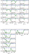 |
Fig. C.5. System at zabs = 5.8441 in the spectrum of PSO J023-02. Upper panel: fit of the detected low-ionization metal lines. Lower panel: fit of the detected high-ionization lines. |
 |
Fig. C.6. System at zabs = 5.8441 in the spectrum of PSO J023-02. Fit of the detected fine-structure lines. |
C.5. PSO J025-11 zabs = 5.7763 PDLA
This system is a PDLA with a two-component velocity structure and a separation from the QSO emission redshift of ∼2866 km s−1. We detected the following ions: O I 1302, C II 1334, Si II 1260, 1304 and 1526, Al II at 1670, Fe II at 2344, 2382 and 2600, and Mg II at 2796, as shown in Fig. C.7. The value of the parameters obtained from the fit of the low ionization lines are shown in Tab. C.5. We carried out the fit by linking the b parameters of all the ions in each of the two components. As for the Al II, which falls in a region with low SNR, we have also linked the redshifts to those of the Si II. The lines of Mg II, on the other hand, fall into the telluric band and are therefore strongly affected by the sky lines, even if they have been partially corrected; only the transition at 2796 could be observed.
Since the system is a PDLA we have also performed the fit of the Lyα absorption line, as described in Sect. 3.4. This line is blended with another Lyα absorption line present in the spectrum, associated with the absorption system at z = 5.8385. From the fit we obtained a column density logNHI = 20.35 ± 0.10, in agreement with the lower limit determined from the rest equivalent width of Mg II 2796 line.
In the system we have also detected high ionization lines, which present a velocity structure characterized by two components of Si IV and C IV (see Fig. C.7 and Tab. C.5). For both components we linked the redshifts and Doppler parameters of the two ions.
Voigt parameters obtained from the fit of the metal lines in the system at zabs = 5.7763 in the spectrum of PSO J025-11.
 |
Fig. C.7. System at zabs = 5.7763 in the spectrum of PSO J025-11. Upper panel: fit of the H I Lyα and Lyβ absorption lines. Middle panel: fit of the detected low-ionization metal lines. Lower panel: fit of the detected high-ionization lines. |
C.6. PSO J025-11 zabs = 5.8385 PDLA
This system is a PDLA with a separation from the QSO emission redshift of ∼127 km s−1. It is characterized by a complex velocity structure. We detected four components of O I 1302 and C II 1334, six components of Si II at 1260, 1304 and 1526, five components of Al II 1670, seven components of Fe II 2382 and 2600 (of which three also detected in Fe II 1608, two also in Fe II 2374 and five also in the transition Fe II 2586), and three components of Mg II 2803, as shown in Fig. C.9. The value of the parameters obtained from the fit of the low ionization lines are shown in Tab. C.6. We performed the fit by linking the Doppler parameter of the velocity profile components that matched in redshift. Oxygen, carbon and magnesium are saturated, therefore their column density was considered a lower limit. The lines of Mg II fall in the telluric band and are therefore strongly affected by the lines of the sky, only three component of the transition at 2803 could be observed, which correspond to the last three components of O I and C II.
We also performed the fit of the H I Lyα absorption line, resulting in a column density logNHI = 21.25 ± 0.10. This line is blended with another Lyα absorption line present in the spectrum, due to the absorption system at z = 5.7763. The H I fit is in agreement with the lower limit for the H I column density based on eq. 5.
In the system we have also detected high ionization lines, which have a velocity structure characterized by three components of Si IV and C IV. We fit the first two components by linking the b parameter of the two ions, while the third leaving this parameter free as well.
Voigt parameters obtained from the fit of the metal lines in the system at zabs = 5.8385 in the spectrum of PSO J025-11.
 |
Fig. C.8. System at zabs = 5.8385 in the spectrum of PSO J025-11. Fit of the H I Lyα and Lyβ absorption lines. |
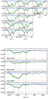 |
Fig. C.9. System at zabs = 5.8385 in the spectrum of PSO J025-11. Upper panel: fit of the detected low-ionization metal lines. Lower panel: fit of the detected high-ionization lines. |
C.7. PSO J108+08 zabs = 5.5624
This system is an intervening DLA composed of a single component, separated from the QSO emission redshift by ∼17400 km s−1. We detected the following ions: O I 1302 and C II 1334, as shown in Fig. C.10. The value of the parameters obtained from the fit of the low ionization lines are shown in Tab. C.7. We performed the fit by linking the redshift of these ions and freezing the parameter b to its minimum value of 5 km s−1 for the visible region of the spectrum. We also derived an upper limit on Si II 1304, Al II 1670, and on Fe II 2382. The Mg II lines fall in a telluric band, and it was not possible to correct the effect of the sky lines at the wavelength at which this absorption occurs.
In this system, we did not detect high ionization lines (see Fig. C.10) thus we derived upper limits on Si IV and C IV. The lower limit on the H I column density derived from eq. 5 is logN(HI)> 18.85.
Voigt parameters obtained from the fit of the metal lines in the system at zabs = 5.5624 in the spectrum of PSO J108+08.
 |
Fig. C.10. System at zabs = 5.5624 in the spectrum of PSO J108+08. Upper panel: fit of the detected low-ionization metal lines, and the region where the absorptions of Si II 1304, Al II 1670 and Fe II 2382 would fall. Lower panel: region where the high ionization lines of Si IV and C IV would fall. |
C.8. SDSS J0818+1722 zabs = 5.7912
This system is an intervening DLA with a velocity structure characterized by three components. The separation from the QSO emission redshift is of ∼8950 km s−1. We detected the following ions: O I 1302, C II 1334, Si II 1260, 1304 and 1526, Fe II 2382 and 2600, as shown in Fig. C.11. The value of the parameters obtained from the fit of the low ionization lines are shown in Tab. C.8. We linked the b parameters of all the ions in each of the three components. The Mg II lines fall in a telluric band and its column density cannot be recovered.
As regards the high ionization lines, in this system we detected the C IV doublet, while we obtained an upper limit for the column density of Si IV, using the transition at 1402 and setting the parameter b at 36 km s−1 like that of C IV (see Fig. C.11 and Tab. C.8).
The lower limit on the H I column density derived from eq. 5 is logN(HI)> 19.51.
This system was already identified by Becker et al. (2011) in a high-resolution spectrum obtained with HIRES at the Keck telescope. They detected O I, C II and Si II, while they did not cover the wavelength region for Fe II and Mg II. The SNR in the regions where C IV and Si IV fall was too low to detect the lines so they determined upper limits. The total column densities for the ions in common between their work and this one are in very good agreement.
Voigt parameters obtained from the fit of the metal lines in the system at zabs = 5.7912 in the spectrum of SDSS J0818+1722.
 |
Fig. C.11. System at zabs = 5.7912 in the spectrum of SDSS J0818+1722. Upper panel: fit of the detected low-ionization metal lines. Lower panel: fit of the detected high-ionization lines. |
C.9. SDSS J0818+1722 zabs = 5.8767
This system is an intervening DLA, with a separation from the QSO emission redshift of ∼5200 km s−1, and a velocity structure consisting of a single component. We detected the ionic transitions due to: O I 1302, C II 1334, Si II 1260, 1304 and 1526, Fe II 2344, 2382, 2586 and 2600, and Mg II at 2796, as shown in Fig. C.13. The value of the parameters obtained from the fit of the low ionization lines are shown in Tab. C.9. We performed the fit by linking the Doppler parameters of all the ions. We also derived an upper limit on Al II 1670. The lines of Mg II, on the other hand, fall into the telluric band and are therefore strongly affected by the lines of the sky; only the stronger transition of the doublet could be observed.
For this system it was possible to fit the H I Lyα absorption line. The obtained column density, logNHI = 20.20 ± 0.10.
High ionization lines were also detected in the system, which have a velocity structure consisting of a single component of Si IV and C IV (see Fig. C.13 and Tab. C.9). We performed the fit by linking the redshift and the b parameter of the two ions.
Also this system was identified and analyzed by Becker et al. (2011) in the high-resolution spectrum obtained with Keck-HIRES. They detected O I, C II and Si II, and determined upper limits on C IV and Si IV lines. The total column densities they obtained are in general good agreement with our estimates. Only in the case of Si II our determination of the column density is 3.6σ larger than their estimate. However, we base our fit on three transitions of the doublet so we are confident that the determination is correct.
Voigt parameters obtained from the fit of the metal lines in the system at zabs = 5.8767 in the spectrum of SDSS J0818+1722.
 |
Fig. C.12. System at zabs = 5.8767 in the spectrum of SDSS J0818+1722. Fit of the H I Lyα and Lyβ absorption lines. |
 |
Fig. C.13. System at zabs = 5.8767 in the spectrum of SDSS J0818+1722. Upper panel: fit of the detected low-ionization metal lines, and region where Al II 1670 absorption would fall. Lower panel: fit of the detected high-ionization lines. |
C.10. PSO J007+04 zabs = 5.9917 PDLA
This system is a single component PDLA, with a separation from the QSO emission redshift of ∼420 km s−1. We detected the ionic transitions due to: O I 1302, C II 1334, Si II 1260, 1304 and 1526, Fe II 2382, as shown in Fig. C.15. The value of the parameters obtained from the fit of the low ionization lines are shown in the Tab. C.10. We performed the fit by linking the b parameters of all the detected ions. We also derived an upper limit on Al II 1670 and on Mg II 2796. Finally, since Mg II is located in a noisy region of the spectrum, the fit of this ion was performed by also linking the redshift with that of Si II.
Since the system is a PDLA we have also performed the fit of the H I Lyα absorption line (see Fig. C.14, as described in Sect. 3.4, obtaining a value of logNHI = 20.40 ± 0.10.
High ionization lines were also detected in the system, with a velocity structure characterized by a single component of both Si IV and C IV (see Fig. C.15 and Tab. C.10). As for the C IV, the transition at 1548 is blended with a line of MgII 2803 at z = 2.8613, while the transition at 1550 is blended with a sky line. We then performed the fit by linking the redshift and the Doppler parameter of Si IV and C IV.
Voigt parameters obtained from the fit of the metal lines in the system at zabs = 5.9917 in the spectrum of PSO J007+04.
 |
Fig. C.14. System at zabs = 5.9917 in the spectrum of PSO J007+04. Fit of the H I Lyα and Lyβ absorption lines. |
 |
Fig. C.15. System at zabs = 5.9917 in the spectrum of PSO J007+04. Upper panel: fit of the detected low-ionization metal lines, and region where the Al II 1670 and Mg II 2796, 2803 absorptions would fall. Lower panel: fit of the detected high-ionization lines. The strong line at the wavelength of C IV 1548 is a Mg II 2803 at z = 2.861. |
C.11. SDSS J2310+1855 zabs = 5.9388 PDLA
This system is a PDLA, with a separation from the QSO emission redshift of ∼2760 km s−1, characterized by a single-component velocity structure. We detected the following ions: O I 1302, C II 1334, Si II 1260, 1304 and 1526, Al II 1670, Fe II 2344, 2382, 2586, 2600, and Mg II 2796, 2803, as shown in Fig. C.16. The value of the parameters obtained from the fit of the low ionization lines are shown in Tab. C.11. We performed the fit by linking the Doppler parameter of all ions, with the exception of Al II and Mg II. The Al II line is superimposed on a sky line while that of Mg II is in a high-noise region, so we fit these ions by fixing the redshift to the same value obtained for Fe II and the b parameter to 7.9 km s−1 as for the other ions. The lines of O I, C II and Mg II are saturated, so we considered their column densities as lower limits.
We have also performed the fit of the H I Lyα and Lyβ absorption lines of this PDLA (see Fig. C.16). The obtained column density, logNHI = 21.00 ± 0.10, is in agreement with the lower limit derived from eq, 5.
In the system, on the other hand, we did not detect high ionization lines (see Fig. C.16), so we derived upper limits on Si IV and C IV.
This system was already analyzed in D’Odorico et al. (2018) using a lower SNR spectrum, the derived column densities are generally in agreement within errors with the old determinations.
Voigt parameters obtained from the fit of the metal lines in the system at zabs = 5.9388 in the spectrum of SDSS J2310+1855.
 |
Fig. C.16. System at zabs = 5.9388 in the spectrum of SDSS J2310+1855. Upper panel: fit of the H I Lyα and Lyβ absorption lines. Middle panel: fit of the detected low-ionization metal lines. Lower panel: region where the high ionization lines of Si IV and C IV would fall. |
Voigt parameters obtained from the fit of the metal lines in the system at zabs = 5.8986 in the spectrum of PSO J158-14.
C.12. PSO J158-14 zabs = 5.8986
This system is an intervening DLA with a single-component velocity structure, separated from the QSO emission redshift by ∼7290 km s−1. The following ions were detected: O I 1302, C II 1334, Si II 1260, 1304, 1526, Al II 1670, Fe II 2344, 2382, and 2600, as shown in Fig. C.17. The values of the parameters obtained from the fit of the low ionization lines are shown in Tab. C.12. The O I line is partially blended with a C IV 1548 line at z = 4.80. We performed the fit by linking the Doppler parameters of all the ions. The Al II line is located in a noisy region of the spectrum, so we fitted this ion by also linking the redshift with that of Si II. Finally, it was not possible to detect the Mg II 2796, 2803 lines as they fall in a strong telluric band which could not be corrected.
A lower limit on H I column density of logNHI > 19.61 is obtained from eq. 5.
High ionization lines were also detected in the system, with a velocity structure consisting of a single component of Si IV and a very weak C IV (see Fig. C.17 and Tab. C.12); we performed the fit by linking the redshift and the parameter b of the two ions.
 |
Fig. C.17. System at zabs = 5.8986 in the spectrum of PSO J158-14. Upper panel: fit of the detected low-ionization metal lines. Lower panel: fit of the detected high-ionization lines. |
Voigt parameters obtained from the fit of the metal lines in the system at zabs = 5.9918 in the spectrum of PSO J239-07.
 |
Fig. C.18. System at zabs = 5.9918 in the spectrum of PSO J239-07. Upper panel: region of the spectrum where the HI Lyα would fall. Middle panel: fit of the detected low-ionization metal lines. Lower panel: region where the high-ionization lines would fall showing the broad absorptions due to N V and C IV. |
C.13. PSO J239-07 zabs = 5.9918 PDLA
This system has a velocity separation of ∼5030 km s−1, at the assumed threshold between intervening and proximate DLAs. It has a single-component velocity structure. We detected the following ions: O I 1302, C II 1334, Si II 1260, 1304, and Mg II 2796, 2803, as shown in Fig. C.18. The value of the parameters obtained from the fit of the low ionization lines are shown in Tab. C.13. The Si II line 1304 is blended with Al III 1862 at z = 3.8962. We performed the fit by linking the redshift and the Doppler parameter of all detected ions. We also derived an upper limit on Al II 1670 and Fe II 2382.
At the redshift of the low ionization lines, we also detected broad absorption lines due to N V and C IV (see Fig. C.18) and we derived an upper limit on Si IV. This QSO was classified as BAL by Bischetti et al. (2022), it shows a complex structure of broad and narrow high-ionization associated systems spanning the velocity range between the QSO systemic redshift and ∼5350 km s−1. The present system could be part of the outflow traced by the high-ionization broad lines, or it could be a neutral intervening system that by chance falls at the same redshift of the outflow. From these observations it is not possible to distinguish between these two scenarios. We decided to choose the latter hypothesis and keep this system in the sample; as a consequence, the detected broad C IV absorption was not associated with the low ionization system and its column density is not considered in the subsequent analysis (e.g., for the computation of the C II/C IV ratio). For the same reason, we did not carry out the fit of the H I Lyα absorption, which, furthermore, would have very limited constraints from the spectrum (see Fig. C.18). However, we estimated a lower limit for the H I column density of logNHI > 18.83 from eq. 5).
Voigt parameters obtained from the fit of the metal lines in the system at zabs = 6.0172 in the spectrum of ULAS J1319+0950.
 |
Fig. C.19. System at zabs = 6.0172 in the spectrum of ULAS J1319+0950. Region of the spectrum where the HI Lyα falls. |
C.14. ULAS J1319+0950 zabs = 6.0172 PDLA
This system is a PDLA, with a separation from the QSO emission redshift of ∼4980 km s−1. We detected single-component velocity features due to the following ions: O I 1302, C II 1334, Si II 1260, 1304, 1526, Al II 1670, Fe II 2382, and Mg II 2796, 2803, as shown in Fig. C.20. The value of the parameters obtained from the fit of the low ionization lines are shown in Tab. C.14. We performed the fit by linking the Doppler parameter of all detected ions, obtaining a value of b = (7 ± 2) km s−1.
In the system, on the other hand, we did not detect high ionization lines (see Fig. C.20). We derived upper limits on Si IV and C IV.
Although the system is a PDLA, we could not perform the fit of the H I Lyα absorption line, because the spectrum does not show a clear damping wing and the fits is not constrained (see Fig. C.20). However, we estimated a lower limit for the H I column density of logNHI > 18.94 from eq. 5.
Simcoe et al. (2011) and D’Odorico et al. (2013) used a FIRE and the same X-SHOOTER spectrum used here, respectively, to study the absorption systems along the line of sight to this QSO but they did not report the detection of this system.
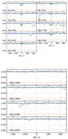 |
Fig. C.20. System at zabs = 6.0172 in the spectrum of ULAS J1319+0950. Upper panel: fit of the detected low-ionization metal lines. Lower panel: region where the high ionization lines of Si IV and C IV would fall. |
C.15. PSO J060+24 zabs = 5.6993
This system is an intervening DLA separated from the QSO emission redshift by ∼20320 km s−1, and characterized by a simple velocity structure consisting of a single component. We detected the following ions: O I 1302, C II 1334, Si II 1304, 1526, Al II 1670, and Fe II 2382, 2586, 2600, as shown in Fig. C.21. The value of the parameters obtained from the fit of the low ionization lines are shown in Tab. C.15. We performed the fit by linking the Doppler parameters of all the ions. The Al II line falls in a noisy spectral region so we fitted it by also linking the redshift with that of Si II. Finally, it was not possible to detect the Mg II doublet as it is lost among the sky lines in a very strong telluric band.
High ionization lines were also detected in the system, which have a velocity structure consisting of a single component of Si IV and C IV (see Fig. C.21 and Tab. C.15); we performed the fit by linking the redshift and the parameter b of the two ions.
The lower limit on H I column density from eq. 5 is logNHI > 19.51.
Voigt parameters obtained from the fit of the metal lines in the system at zabs = 5.6993 in the spectrum of PSO J060+24.
Voigt parameters obtained from the fit of the metal lines in the system at zabs = 5.8677 in the spectrum of PSO J065-26.
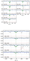 |
Fig. C.21. System at zabs = 5.6993 in the spectrum of PSO J060+24. Upper panel: fit of the detected low-ionization metal lines. Lower panel: fit of the detected high-ionization lines. |
C.16. PSO J065-26 zabs = 5.8677
This intervening DLA has a velocity structure characterized by two components, with an average separation from the QSO emission redshift of ∼13620 km s−1. We detected the following ions: O I 1302, C II 1334, Si II 1304, 1526, Al II 1670, Fe II 2344, 2382, 2586, 2600, and Mg II 2803, as shown in Fig. C.22. The value of the parameters obtained from the fit of the low ionization lines are shown in Tab. C.16. We linked the b parameters of all the ions in each of the two components, except the Mg II. The lines of Mg II fall into the telluric band and are therefore strongly affected by the lines of the sky; for this reason we could detect only one component of the transition at 2803.
C IV and Si IV doublets are not observed at the redshift of this system (see Fig. C.22), therefore we derived upper limits for their column densities.
Finally, we used eq. 5 to estimate a lower limit on the H I column density of logNHI > 20.02.
 |
Fig. C.22. System at zabs = 5.8677 in the spectrum of PSO J065-26. Upper panel: fit of the detected low-ionization metal lines. Lower panel: region where the high ionization lines of Si IV and C IV would fall. |
C.17. PSO J065-26 zabs = 6.1208 PDLA
This system is a PDLA with a separation from the QSO emission redshift of about ∼2780 km s−1, and a velocity structure characterized by two components. We detected the following ions: S II 1250, 1253, 1259, O I 1302, C II 1334, Si II 1260, 1304, 1526, Al II 1670, Fe II 2344, 2374, 2382, and Mg II 2796, 2803, as shown in Fig. C.24. The value of the parameters obtained from the fit of the low ionization lines are shown in Tab. C.17. We linked the Doppler parameters of all the ions in each component. Oxygen, carbon and magnesium are saturated, therefore their column densities were considered as lower limits.
From eq. 5, we derived a lower limit on the H I column density of logNHI > 20.42. Since this system is a PDLA, we performed also the fit of the H I Lyα absorption line which however comprises both this system and the next one at z = 6.1263, which are separated by less than 250 km s−1. Furthermore, it was not possible to obtain an H I column density larger than 19.9 independently of the adopted continuum. This suggests that these systems are affected by partial coverage, and therefore we have not considered the value obtained from this fit.
C IV and Si IV doublets are not observed at the redshift of this system (see Fig. C.24), therefore we derived upper limits for their column densities.
Voigt parameters obtained from the fit of the metal lines in the system at zabs = 6.1208 in the spectrum of PSO J065-26.
 |
Fig. C.23. Fit of the H I Lyα and Lyβ absorption lines corresponding to the systems at zabs = 6.1208 and 6.1263 in the spectrum of PSO J065-26. |
 |
Fig. C.24. System at zabs = 6.1208 in the spectrum of PSO J065-26. Upper panel: fit of the H I Lyα and Lyβ absorption lines together with the z = 6.1263 system. Middle panel: fit of the detected low-ionization metal lines. Lower panel: region where the high ionization lines of Si IV and C IV would fall. |
C.18. PSO J065-26 zabs = 6.1263 PDLA
This system is PDLA with a separation from the QSO emission redshift of about ∼2540 km s−1, and a velocity structure characterized by three components. It is separated by only ∼250km s−1 from the system described in the previous section. Nonetheless, we decided to describe the two systems separately, in particular, because the one at larger velocities from the QSO did not show associated high-ionization absorption lines, while this one does. We detected the following ions: S II 1253, 1259, O I 1302, C II 1334, Si II 1260, 1304, 1526, Al II 1670, Fe II 2344, 2374, 2382, and Mg II 2796, 2803, as shown in Fig. C.25. The value of the parameters obtained from the fit of the low ionization lines are shown in Tab. C.18. We linked the Doppler parameters of all the ions in each component. Carbon and magnesium are saturated, therefore their column densities were considered as lower limit.
Furthermore, we derived a lower limit on the H I column density of logNHI > 19.52 from eq. 5, and we performed the fit of the H I Lyα absorption line as described in the previous section.
High ionization lines were also detected in the system, which have a velocity structure consisting of a single component of Si IV and C IV (see Fig. C.25 and Tab. C.18); we performed the fit by linking the redshift and the parameter b of the two ions.
Voigt parameters obtained from the fit of the metal lines in the system at zabs = 6.1263 in the spectrum of PSO J065-26.
 |
Fig. C.25. System at zabs = 6.1263 in the spectrum of PSO J065-26. Upper panel: fit of the detected low-ionization metal lines. Lower panel: fit of the detected high-ionization lines. |
C.19. SDSS J0100+2802 zabs = 5.7974
This literature QSO has the highest SNR spectrum of the sample and is the only one which shows four O I absorption systems. The system described here is an intervening DLA at ∼22440 km s−1 from the QSO emission redshift, characterized by a simple velocity structure consisting of a single component. We detected the following ions: O I 1302, C II 1334, Si II 1304, 1526, Al II 1670, and Fe II 1608,2344,2374,2382, 2586, 2600, as shown in Fig. C.26. The values of the parameters obtained from the fit of the low ionization lines are shown in Tab. C.19. The O I line is blended with a Lyα line at z = 6.2792, and we performed the fit by linking the Doppler parameters of all the ions.
High ionization lines were also detected in the system, which have a velocity structure consisting of a single component of Si IV and C IV (see Fig. C.26 and Tab. C.19). We performed the fit by linking the redshift and the parameter b of the two ions.
The lower limit on the H I column density obtained from eq. 5 is logNHI > 19.64.
Voigt parameters obtained from the fit of the metal lines in the system at zabs = 5.7974 in the spectrum of SDSS J0100+2802.
 |
Fig. C.26. System at zabs = 5.7974 in the spectrum of SDSS J0100+2802. Upper panel: fit of the detected low-ionization metal lines. Lower panel: fit of the detected high-ionization lines. |
C.20. SDSS J0100+2802 zabs = 5.9450
The system described here is an intervening DLA at ∼16030 km s−1 from the QSO emission redshift, characterized by a simple velocity structure consisting of a single component. We detected the following ions: O I 1302, C II 1334, Si II 1304, 1526, Al II 1670, Fe II 2382, 2600, and Mg II 2796, 2803, as shown in Fig. C.27. The value of the parameters obtained from the fit of the low ionization lines are shown in Tab. C.20. We performed the fit by linking the Doppler parameters of all the ions.
High ionization lines were also detected in the system, which have a velocity structure consisting of a single component of Si IV and C IV and a shift of ∼66 km s−1 with respect to the low-ionization lines (see Fig. C.27 and Tab. C.20). We performed the fit by linking the redshift and the parameter b of the two ions.
Finally, we estimated a lower limit for the H I column density of logNHI > 18.45 from the eq. 5.
Voigt parameters obtained from the fit of the metal lines in the system at zabs = 5.9450 in the spectrum of SDSS J0100+2802.
 |
Fig. C.27. System at zabs = 5.9450 in the spectrum of SDSS J0100+2802. Upper panel: fit of the detected low-ionization metal lines. Lower panel: fit of the detected high-ionization lines. |
C.21. SDSS J0100+2802 zabs = 6.1114
This system is an intervening DLA, with a separation from the QSO emission redshift of ∼8940 km s−1. We detected two components of O I 1302, C II 1334, Si II 1260, 1304, 1526, and Mg II 2796, 2803, and a single component of Al II 1670, and Fe II 1608, 2344, 2382, as shown in Fig. C.28. The value of the parameters obtained from the fit of the low ionization lines are shown in Tab. C.21. The line of Si II 1526 is blended with the C IV 1548 line at z = 6.01. We performed the fit by linking the b parameters of all the ions in each of the two components.
In this system, on the other hand, we did not detect high ionization lines, we have therefore derived an upper limit on Si IV and C IV.
Finally, from eq. 5, we derived a lower limit for the H I column density of logNHI > 19.70.
Voigt parameters obtained from the fit of the metal lines in the system at zabs = 6.1114 in the spectrum of SDSS J0100+2802.
 |
Fig. C.28. System at zabs = 6.1114 in the spectrum of SDSS J0100+2802. Upper panel: fit of the detected low-ionization metal lines. Lower panel: region where the high ionization lines of Si IV and C IV would fall. |
C.22. SDSS J0100+2802 zabs = 6.1434
This system is separated from the QSO emission redshift by ∼7600 km s−1. We detected the following ions: O I 1302, C II 1334, Si II 1260, 1304 and 1526, Al II 1670, Fe II 1608, 2344, 2382, and Mg II 2796 and 2803, as shown in Fig. C.30. The value of the parameters obtained from the fit of the low ionization lines are shown in Tab. C.22. We performed the fit by linking the Doppler parameters of all the ions.
For this system, we could carry out the fit of the H I Lyα absorption line, which resulted in logNHI = 20.20 ± 0.10 (see Fig. C.29.
Also for this system, we did not detect high ionization lines, we have therefore derived an upper limit on Si IV and C IV.
Voigt parameters obtained from the fit of the metal lines in the system at zabs = 6.1434 in the spectrum of SDSS J0100+2802.
 |
Fig. C.29. System at zabs = 6.1434 in the spectrum of SDSS J0100+2802. Fit of the H I Lyα and Lyβ absorption lines. |
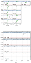 |
Fig. C.30. System at zabs = 6.1434 in the spectrum of SDSS J0100+2802. Upper panel: fit of the detected low-ionization metal lines. Lower panel: region where the high ionization lines of Si IV and C IV would fall. |
C.23. DELS J1535+1943 zabs = 5.8990
This system is an intervening DLA with a separation from the QSO emission redshift of ∼20210 km s−1. It has a complex velocity structure characterized by three components observed in O I 1302, C II 1334, and Mg II 2803 (the profile of the Mg II 2796 line is partially occulted by a telluric absorption), and two components in Si II 1304, 1526, Fe II 2344, 2382 and 2600, as shown in Fig. C.31. The value of the parameters obtained from the fit of the low ionization lines are shown in Tab. C.23.
The O I absorption falls at the beginning of the Lyα forest. It is still visible thanks to the presence of the QSO Lyα line in emission, but partially blended with some Lyα lines. Therefore, we consider this system in our sample of DLA analogs, but since the O I column density is too uncertain, we did not use it in the subsequent analysis. For this reason, we could not derive an estimate for the H I column density lower limit.
As for the other ions, we fitted the first component by linking the redshift and the Doppler parameter of all ions; for the the second component, the redshift of all ions except C II were linked together, and the Doppler parameter was fixed at its minimum value b = 6 km s−1 for Si II and Fe II. Finally, we detected a third component in C II and Mg II which was fitted by linking their b parameters.
In the system we have also detected high ionization lines, which have a velocity structure characterized by three components of both Si IV and C IV (see Fig. C.31 and Tab. C.23). We performed the fit of all the components by linking the redshift and the b parameter of the two ions.
Voigt parameters obtained from the fit of the metal lines in the system at zabs = 5.8990 in the spectrum of DELS J1535+1943.
 |
Fig. C.31. System at zabs = 5.8990 in the spectrum of DELS J1535+1943. Upper panel: fit of the detected low-ionization metal lines. Lower panel: fit of the detected high-ionization lines. |
C.24. PSO J183+05 zabs = 6.0642
This system is an intervening DLA, with a separation from the QSO emission redshift of ∼15470 km s−1. We detected a velocity structure with two components for the transitions due to O I 1302, C II 1334, Si II 1304, 1526, Al II 1670, and Fe II 2344, 2382 Å while Mg II 2796, 2803 shows an additional broad component, as shown in Fig. C.32. The value of the parameters obtained from the fit of the low ionization lines are reported in Tab. C.24. We linked the b parameters of all the ions in each component, with the exception of the first component of Mg II for which we have fixed the value to b = 8 km s−1.
In the system we have also detected high ionization lines, which have a velocity structure characterized by three components of both Si IV and C IV covering a slightly broader velocity interval than the low ionization lines (see Fig. C.32 and Tab. C.24). We performed the fit of all the components by linking the redshift and the b parameter of the two ions.
Finally, we estimated a lower limit for the H I column density based on eq. 5 of logNHI > 19.53.
Voigt parameters obtained from the fit of the metal lines in the system at zabs = 6.0642 in the spectrum of PSO J183+05.
 |
Fig. C.32. System at zabs = 6.0642 in the spectrum of PSO J183+05. Upper panel: fit of the detected low-ionization metal lines. Lower panel: fit of the detected high-ionization lines. |
C.25. PSO J183+05 zabs = 6.4041 PDLA
This system is a PDLA, with a separation from the QSO emission redshift of ∼1390 km s−1, which presents a velocity structure characterized by two components. We detected the following ions: O I 1302, C II 1334, Si II 1260, 1304, 1526, Al II 1670, Fe II 2344, 2374, 2382, and Mg II 2796, 2803, as shown in Fig. C.33. The value of the parameters obtained from the fit of the low ionization lines are shown in Tab. C.25. We performed the fit by linking the redshift and the Doppler parameter of all the ions for the weaker component, and linking only the Doppler parameter for the stronger one. The lines of Mg II are saturated, so we considered the column densities as lower limits.
 |
Fig. C.33. System at zabs = 6.4041 in the spectrum of PSO J183+05. Upper panel: fit of the H I Lyα and Lyβ absorption lines. Middle panel: fit of the detected low-ionization metal lines. Lower panel: region where the high ionization lines of Si IV and C IV would fall. |
We have also performed the fit of the H I Lyα absorption line of this PDLA, as described in Sect. 3.4, and we obtained a column density of logNHI = 20.60 ± 0.10.
In the system, on the other hand, we did not detect high ionization lines (see Fig. C.33) and we derived an upper limit on Si IV and C IV.
This system was already identified and analyzed in Bañados et al. (2019), based on a FIRE spectrum at lower SNR than our X-SHOOTER one. The lower resolution of the FIRE spectrum did not allow to distinguish the velocity structure of the system. Bañados et al. (2019) determined for each transition the equivalent width and then determined the column densities with the Apparent Optical Depth (AOD) method. On average, we find total column densities (see Tab. A.2) larger by 0.3 dex (0.2 dex if we exclude the heavily saturated Mg II) which is not always consistent with the reported errors. On the other hand, we derive an H I column density slightly smaller than the one measured from the FIRE spectrum (but within uncertainties) although the adopted continuum looks quite similar. As a consequence of these discrepancies, we derive metal abundances larger than those by Bañados et al. (2019) by ∼0.2 − 0.4 dex.
Voigt parameters obtained from the fit of the metal lines in the system at zabs = 6.4041 in the spectrum of PSO J183+05.
Voigt parameters obtained from the fit of the metal lines in the system at zabs = 6.2743 in the spectrum of WISEA J0439+1634.
C.26. WISEA J0439+1634 zabs = 6.2743
This system is a single component DLA, separated from the QSO emission redshift by ∼9910 km s−1. The following ionic transitions were detected: O I 1302, C II 1334, Si II 1260, 1304, as shown in Fig. C.34. The value of the parameters obtained from the fit of the low ionization lines are shown in Tab. C.26. We performed the fit by linking the redshift of these ions and freezing the parameter b to its minimum value: 6 km s−1 for O I, C II and Si II which fall in the visible region of the spectrum. We also derived an upper limit on Al II 1670, Fe II 2382 and Mg II 2796 by fixing the Doppler parameter to b = 7 km s−1 as they are in the infrared region of the spectrum.
 |
Fig. C.34. System at zabs = 6.2743 in the spectrum of WISEA J0439+1634. Upper panel: fit of the detected low-ionization metal lines, and region where Al II 1670, Fe II 2382 and Mg II 2796 and 2803 absorptions would fall. Lower panel: region where the high ionization lines of Si IV and C IV would fall. |
Voigt parameters obtained from the fit of the metal lines in the system at zabs = 6.1228 in the spectrum of VDES J0224-4711.
We did not detect high ionization lines at the redshift of the low ionization ones, and we have therefore derived an upper limit on Si IV and C IV. On the other hand, we observe a broad CIV absorption, with b = 168 ± 5 km s−1, at z = 6.2838 with a separation of ∼400 km s−1 from the low ionization lines. We assume that this C IV is not related with the low ionization system and is probably part of the complex BAL system characterizing the spectrum of this QSO.
We note that this absorption system was studied also in Christensen et al. (2023) based on a JWST-NIRSpec spectrum with a resolving power R 2700. Lines are not resolved in this spectrum, and the authors derived column densities from equivalent widths assuming they are on the linear part of the curve of growth. These column densities are in general much larger than those determined in our work, e.g., logN(OI)≃14.22, logN(CII)≃13.88 (considered as an upper limit), logN(SiII1304)≃13.8 and logN(SiII1260)≃12.56 (the authors did not specify how they treated these two different values). What is relevant is that our determination of column densities provides relative chemical abundances which are not so extreme (see Tab. B.2 and Vanni et al. 2024): the system falls in a region of the [Si/O] vs. [C/O] plot which is compatible with the enrichment from Pop II SNe.
 |
Fig. C.35. System at zabs = 6.1228 in the spectrum of VDES J0224-4711. Upper panel: fit of the detected low-ionization metal lines, and region where Al II 1670 absorption would fall. Lower panel: region where the high ionization lines of Si IV and C IV would fall. |
C.27. VDES J0224-4711 zabs = 6.1228
This system is an intervening DLA, with a separation from the QSO emission redshift of ∼16450 km s−1. We detected a low ionization system with a single velocity component showing the following ions: O I 1302, C II 1334, Si II 1304, 1526, Fe II 2382, and Mg II 2796, 2803, as shown in Fig. C.35. The value of the parameters obtained from the fit of the low ionization lines are shown in Tab. C.27. We performed the fit by linking the Doppler parameters of all the ions, and we also derived an upper limit on Al II 1670.
 |
Fig. C.36. System at zabs = 6.0611 in the spectrum of PSO J036+03.Upper panel: fit of the detected low-ionization metal lines, and region where Fe II 2382 absorption would fall. Lower panel: fit of the detected high-ionization lines. |
 |
Fig. C.37. System at zabs = 6.3784 in the spectrum of DELS J0923+0402. Fit of the detected low-ionization metal lines, and region where Al II 1670 and Fe II 2382 absorptions would fall. |
C IV and Si IV doublets are not observed at the redshift of this system (see Fig. C.35), therefore we derived upper limits for their column densities.
Finally, we estimated a lower limit for the H I column density based on eq. 5 of logNHI > 19.47.
C.28. PSO J036+03 zabs = 6.0611
This system is an intervening DLA, with a separation from the QSO emission redshift of ∼19660 km s−1, and is characterized by a simple velocity structure consisting of a single component. We detected the following ions: O I 1302, C II 1334, Si II 1304, 1526, Al II 1670 and Mg II 2796, 2803, as shown in Fig. C.36. The value of the parameters obtained from the fit of the low ionization lines are shown in Tab. C.28. The transition of Si II 1304 is blended with a C II line at z = 5.9023, while the Si II transition at 1526 is very weak. We then linked the redshift of Si II with that of O I and C II. Also the line of Al II 1670 is very weak so, also in this case, we have linked the redshift with that of O I and C II. We performed the fit by linking the parameter b of all the ions. We also derived an upper limit on Fe II at 2382.
High ionization lines were detected in the system, with a single component of Si IV and C IV at the same redshift of the low-ionization lines (see Fig. C.36 and Tab. C.28). We performed the fit by linking the redshift and the parameter b of the two ions.
Finally, we obtained a lower limit for the H I column density of logNHI > 19.89, derived from eq. 5.
Voigt parameters obtained from the fit of the metal lines in the system at zabs = 6.0611 in the spectrum of PSO J036+03.
Voigt parameters obtained from the fit of the metal lines in the system at zabs = 6.3784 in the spectrum of DELS J0923+0402.
C.29. DELS J0923+0402 zabs = 6.3784
This DLA falls at ∼10170 km s−1, and it shows a velocity structure consisting of a single component. We detected the following ions: O I 1302, C II 1334, Si II 1260 and Mg II 2796, 2803, as shown in Fig. C.37. The value of the parameters obtained from the fit of the low ionization lines are shown in Tab. C.29. We performed the fit by linking the redshift of these ions and freezing the parameter b to its minimum value: 6 km s−1 for the transitions O I, C II and Si II falling in the VIS spectrum, and 7 km s−1 for Mg II which is observed in the NIR spectrum. We also derived an upper limit on Al II 1670 and Fe II 2382.
Furthermore, from eq. 5 we derived a lower limit for the H I column density of logNHI > 19.57.
The C IV and Si IV doublets for this system are falling in the trough of the strong BAL systems present in the spectrum of this object (see Bischetti et al. 2022), therefore their presence cannot be established. Alternatively, the system could be due to a small neutral clump of gas entrained in the strong BAL outflows. As for the system at z = 5.9918 in PSO J239-07, the intrinsic or intervening nature of this system cannot be established from the present observations, thus we assume that it is intervening and we consider it in our analysis.
All Tables
Chemical abundances relative to iron of the elements detected in the observed O I systems.
Weighted average of the chemical abundances of the VMP-DLAs at 2 ≤ z ≤ 4.5 and DLA-analogs at 4.5 < z ≤ 6.5.
Properties of the three systems in our sample presenting the largest [C/O] and [Si/O] abundance ratios.
Column density ratios of C II to C IV, and Si II to Si IV, in the detected O I systems.
Logarithm of the total column densities (in cm−2) of ions detected in the observed O I systems.
Chemical abundance of elements detected in low ionization systems where the column density of H I could be estimated.
Chemical abundances relative to oxygen of the elements detected in the observed low ionization systems.
Voigt parameters obtained from the fit of the metal lines in the system at zabs = 5.4400 in the spectrum of PSO J308-27.
Voigt parameters obtained from the fit of the metal lines in the system at zabs = 5.6268 in the spectrum of PSO J308-27.
Voigt parameters obtained from the fit of the metal lines in the system at zabs = 5.4869 in the spectrum of PSO J023-02.
Voigt parameters obtained from the fit of the metal lines in the system at zabs = 5.8441 in the spectrum of PSO J023-02.
Voigt parameters obtained from the fit of the metal lines in the system at zabs = 5.7763 in the spectrum of PSO J025-11.
Voigt parameters obtained from the fit of the metal lines in the system at zabs = 5.8385 in the spectrum of PSO J025-11.
Voigt parameters obtained from the fit of the metal lines in the system at zabs = 5.5624 in the spectrum of PSO J108+08.
Voigt parameters obtained from the fit of the metal lines in the system at zabs = 5.7912 in the spectrum of SDSS J0818+1722.
Voigt parameters obtained from the fit of the metal lines in the system at zabs = 5.8767 in the spectrum of SDSS J0818+1722.
Voigt parameters obtained from the fit of the metal lines in the system at zabs = 5.9917 in the spectrum of PSO J007+04.
Voigt parameters obtained from the fit of the metal lines in the system at zabs = 5.9388 in the spectrum of SDSS J2310+1855.
Voigt parameters obtained from the fit of the metal lines in the system at zabs = 5.8986 in the spectrum of PSO J158-14.
Voigt parameters obtained from the fit of the metal lines in the system at zabs = 5.9918 in the spectrum of PSO J239-07.
Voigt parameters obtained from the fit of the metal lines in the system at zabs = 6.0172 in the spectrum of ULAS J1319+0950.
Voigt parameters obtained from the fit of the metal lines in the system at zabs = 5.6993 in the spectrum of PSO J060+24.
Voigt parameters obtained from the fit of the metal lines in the system at zabs = 5.8677 in the spectrum of PSO J065-26.
Voigt parameters obtained from the fit of the metal lines in the system at zabs = 6.1208 in the spectrum of PSO J065-26.
Voigt parameters obtained from the fit of the metal lines in the system at zabs = 6.1263 in the spectrum of PSO J065-26.
Voigt parameters obtained from the fit of the metal lines in the system at zabs = 5.7974 in the spectrum of SDSS J0100+2802.
Voigt parameters obtained from the fit of the metal lines in the system at zabs = 5.9450 in the spectrum of SDSS J0100+2802.
Voigt parameters obtained from the fit of the metal lines in the system at zabs = 6.1114 in the spectrum of SDSS J0100+2802.
Voigt parameters obtained from the fit of the metal lines in the system at zabs = 6.1434 in the spectrum of SDSS J0100+2802.
Voigt parameters obtained from the fit of the metal lines in the system at zabs = 5.8990 in the spectrum of DELS J1535+1943.
Voigt parameters obtained from the fit of the metal lines in the system at zabs = 6.0642 in the spectrum of PSO J183+05.
Voigt parameters obtained from the fit of the metal lines in the system at zabs = 6.4041 in the spectrum of PSO J183+05.
Voigt parameters obtained from the fit of the metal lines in the system at zabs = 6.2743 in the spectrum of WISEA J0439+1634.
Voigt parameters obtained from the fit of the metal lines in the system at zabs = 6.1228 in the spectrum of VDES J0224-4711.
Voigt parameters obtained from the fit of the metal lines in the system at zabs = 6.0611 in the spectrum of PSO J036+03.
Voigt parameters obtained from the fit of the metal lines in the system at zabs = 6.3784 in the spectrum of DELS J0923+0402.
All Figures
|
Fig. 1. Comparison between two absorption lines fitted with Voigt profiles in XQR-30 (upper panels; black line: observed spectrum; red line: observed error; blue line: continuum level; green line: Voigt profile fit) and their theoretical profiles without the convolution with the instrumental broadening (lower panels). The theoretical profile of the line on the left is saturated, while the theoretical profile of the line on the right is not. |
| In the text | |
|
Fig. 2. Log N(O I) as a function of log NH I for the VMP DLAs of Cooke et al. (2011, triangles). The color of the triangles refers to their metallicity measured as [Fe/H] and reported in the side band. The solid black lines are approximately marking metallicities of [Fe/H] ≃ − 2, −3 and −4 (from top to bottom). The dotted black line indicates the column density threshold defining DLAs. The red lower limits on log NH I are the O I absorbers in our sample, red circles indicate PDLA systems. Dark-red crosses mark estimated log NH I for the latter systems, obtained from the fit of the red damping wing of the absorption. |
| In the text | |
|
Fig. 3. Region of the spectrum of the QSO SDSS J2310+1855 corresponding to the Lyα emission. The black line is the observed spectrum and the red one is the observed error. The blue line is the intrinsic emission spectrum modeled with a template (see text), while the green line is the fit of the H I Lyα absorption line for the PDLA at z = 5.9388. |
| In the text | |
|
Fig. 4. Abundances relative to iron of the elements detected in our O I systems. In the panels, PDLAs (red filled circles) are distinguished from intervening DLAs (orange empty circles). The orange shaded box (red shaded box) represents the weighted average value of the DLA (PDLA) abundances with the relative dispersion, calculated as the standard deviation of the sample mean. |
| In the text | |
|
Fig. 5. Comparison of some of the relative abundances of the O I systems/DLAs at high redshift (z > 4.5) found in this work (red dots), in Becker et al. (2012) (blue squares), and Poudel et al. (2018, 2020) (green diamonds). Dotted lines mark the solar abundance values. We report also the predictions of the simulations by Kulkarni et al. (2013) at z = 6, the three models are described in greater detail the text. Model 1 assigns a 1–100 M⊙ Salpeter IMF to Pop III stars. This is 35–100 M⊙ Salpeter in case of model 2 and 100–260 M⊙ Salpeter for model 3. The prediction of model 1 is the light blue dot at the junction of the lines of model 2 and 3. |
| In the text | |
|
Fig. 6. Relative abundances of DLA systems at z > 2, as a function of redshift. The figure shows the DLA analogs studied in this work (solid red dots), in Becker et al. (2012, solid blue squares) and in Poudel et al. (2018, 2020, solid green diamonds), and the VMP-DLAs analyzed in Cooke et al. (2011, solid black triangles) with the exception of the systems identified in the QSOs J0035−0918 and J1558−0031, and those in Dutta et al. (2014, solid plum inverted triangles) in the QSOs J0035−0918 and J0953−0504. The shaded regions are centred on the weighted average values and represent the standard deviation of the sample (light gray band) and of the sample mean (dark gray band) for the systems in the two redshift bins: 2 ≤ z ≤ 4.5 and 4.5 < z ≤ 6.5. |
| In the text | |
|
Fig. 7. Comparison between the maximum extent of [C/O] (left panel) and [Si/O] (right panel) ISM ratios predicted in the model by Vanni et al. (2024, shaded area) and the measured abundance ratios in absorbers at different redshifts (points with errorbars as in Fig. 6). In each panel the colored areas show the contribution of Pop III stars to the chemical enrichment: 100% (yellow), 90% (orange), 60% (pink), 30% (purple) and ≤0.01% (dark grey: Limongi & Chieffi 2018; light grey: Woosley & Weaver 1995). Only the environments with [O/H] > − 4 are considered. The three remarkable systems with [C/O] > 0.35 and [Si/O] > 0.50 are highlighted using different symbols and black contours: PSO J025−11 at z = 5.7763 (square), SDSS J0100+2802 at z = 5.9450 (star) and PSO J065−26 at z = 6.1263 (diamond). |
| In the text | |
|
Fig. 8. Comparison between different chemical abundance ratios measured in the considered sample of z > 4.5 DLA-analogs (points with errorbars as in Fig. 5) and predicted in the model by Vanni et al. (2024, shaded area). Shaded areas are colored depending upon the contribution level of Pop III stars to the chemical enrichment: 100% (yellow), 90% (orange), 60% (pink), 30% (purple) and ≤0.01% (dark grey: Limongi & Chieffi 2018; light grey: Woosley & Weaver 1995). Only the environments with [O/H] > − 4 are considered. The three remarkable systems with [C/O] > 0.35 and [Si/O] > 0.50 are highlighted using different symbols and black contours: PSO J025−11 at z = 5.7763 (square), SDSS J0100+2802 at z = 5.9450 (star) and PSO J065−26 at z = 6.1263 (diamond). |
| In the text | |
|
Fig. 9. Ratio of C II/C IV (left panels) and Si II/Si IV (right panels) column densities as a function of redshift (upper panels) and velocity separation from the systemic redshift of the QSO (lower panels) for our sample of O I systems. The dotted vertical lines in the upper panels are drawn at z = 5.7, the limit beyond which the low ionization phase is expected to dominate in the gas (Cooper et al. 2019). The vertical dotted lines in the lower panels mark a velocity separation of 5000 km s−1, which separates PDLAs from intervening DLAs. In each panel, the three systems with black contours (diamond, square and star) are the same highlighted in Figs. 7 and 8. |
| In the text | |
|
Fig. C.1. System at zabs = 5.4400 in the spectrum of PSO J308-27. Upper panel: fit of the detected low-ionization metal lines, and region where Al II 1670 absorption would fall. Lower panel: fit of the detected high-ionization lines. |
| In the text | |
|
Fig. C.2. System at zabs = 5.6268 in the spectrum of PSO J308-27. Upper panel: fit of the detected low-ionization metal lines. Lower panel: fit of the detected high-ionization lines. |
| In the text | |
|
Fig. C.3. System at zabs = 5.4869 in the spectrum of PSO J023-02. Upper panel: fit of the detected low-ionization metal lines, and the region where the absorptions of Si II 1526 and Al II 1670 would fall. Lower panel: region where the high ionization lines of Si IV and C IV would fall. |
| In the text | |
|
Fig. C.4. System at zabs = 5.8441 in the spectrum of PSO J023-02. Fit of the H I Lyα absorption line |
| In the text | |
|
Fig. C.5. System at zabs = 5.8441 in the spectrum of PSO J023-02. Upper panel: fit of the detected low-ionization metal lines. Lower panel: fit of the detected high-ionization lines. |
| In the text | |
|
Fig. C.6. System at zabs = 5.8441 in the spectrum of PSO J023-02. Fit of the detected fine-structure lines. |
| In the text | |
|
Fig. C.7. System at zabs = 5.7763 in the spectrum of PSO J025-11. Upper panel: fit of the H I Lyα and Lyβ absorption lines. Middle panel: fit of the detected low-ionization metal lines. Lower panel: fit of the detected high-ionization lines. |
| In the text | |
|
Fig. C.8. System at zabs = 5.8385 in the spectrum of PSO J025-11. Fit of the H I Lyα and Lyβ absorption lines. |
| In the text | |
|
Fig. C.9. System at zabs = 5.8385 in the spectrum of PSO J025-11. Upper panel: fit of the detected low-ionization metal lines. Lower panel: fit of the detected high-ionization lines. |
| In the text | |
|
Fig. C.10. System at zabs = 5.5624 in the spectrum of PSO J108+08. Upper panel: fit of the detected low-ionization metal lines, and the region where the absorptions of Si II 1304, Al II 1670 and Fe II 2382 would fall. Lower panel: region where the high ionization lines of Si IV and C IV would fall. |
| In the text | |
|
Fig. C.11. System at zabs = 5.7912 in the spectrum of SDSS J0818+1722. Upper panel: fit of the detected low-ionization metal lines. Lower panel: fit of the detected high-ionization lines. |
| In the text | |
|
Fig. C.12. System at zabs = 5.8767 in the spectrum of SDSS J0818+1722. Fit of the H I Lyα and Lyβ absorption lines. |
| In the text | |
|
Fig. C.13. System at zabs = 5.8767 in the spectrum of SDSS J0818+1722. Upper panel: fit of the detected low-ionization metal lines, and region where Al II 1670 absorption would fall. Lower panel: fit of the detected high-ionization lines. |
| In the text | |
|
Fig. C.14. System at zabs = 5.9917 in the spectrum of PSO J007+04. Fit of the H I Lyα and Lyβ absorption lines. |
| In the text | |
|
Fig. C.15. System at zabs = 5.9917 in the spectrum of PSO J007+04. Upper panel: fit of the detected low-ionization metal lines, and region where the Al II 1670 and Mg II 2796, 2803 absorptions would fall. Lower panel: fit of the detected high-ionization lines. The strong line at the wavelength of C IV 1548 is a Mg II 2803 at z = 2.861. |
| In the text | |
|
Fig. C.16. System at zabs = 5.9388 in the spectrum of SDSS J2310+1855. Upper panel: fit of the H I Lyα and Lyβ absorption lines. Middle panel: fit of the detected low-ionization metal lines. Lower panel: region where the high ionization lines of Si IV and C IV would fall. |
| In the text | |
|
Fig. C.17. System at zabs = 5.8986 in the spectrum of PSO J158-14. Upper panel: fit of the detected low-ionization metal lines. Lower panel: fit of the detected high-ionization lines. |
| In the text | |
|
Fig. C.18. System at zabs = 5.9918 in the spectrum of PSO J239-07. Upper panel: region of the spectrum where the HI Lyα would fall. Middle panel: fit of the detected low-ionization metal lines. Lower panel: region where the high-ionization lines would fall showing the broad absorptions due to N V and C IV. |
| In the text | |
|
Fig. C.19. System at zabs = 6.0172 in the spectrum of ULAS J1319+0950. Region of the spectrum where the HI Lyα falls. |
| In the text | |
|
Fig. C.20. System at zabs = 6.0172 in the spectrum of ULAS J1319+0950. Upper panel: fit of the detected low-ionization metal lines. Lower panel: region where the high ionization lines of Si IV and C IV would fall. |
| In the text | |
|
Fig. C.21. System at zabs = 5.6993 in the spectrum of PSO J060+24. Upper panel: fit of the detected low-ionization metal lines. Lower panel: fit of the detected high-ionization lines. |
| In the text | |
|
Fig. C.22. System at zabs = 5.8677 in the spectrum of PSO J065-26. Upper panel: fit of the detected low-ionization metal lines. Lower panel: region where the high ionization lines of Si IV and C IV would fall. |
| In the text | |
|
Fig. C.23. Fit of the H I Lyα and Lyβ absorption lines corresponding to the systems at zabs = 6.1208 and 6.1263 in the spectrum of PSO J065-26. |
| In the text | |
|
Fig. C.24. System at zabs = 6.1208 in the spectrum of PSO J065-26. Upper panel: fit of the H I Lyα and Lyβ absorption lines together with the z = 6.1263 system. Middle panel: fit of the detected low-ionization metal lines. Lower panel: region where the high ionization lines of Si IV and C IV would fall. |
| In the text | |
|
Fig. C.25. System at zabs = 6.1263 in the spectrum of PSO J065-26. Upper panel: fit of the detected low-ionization metal lines. Lower panel: fit of the detected high-ionization lines. |
| In the text | |
|
Fig. C.26. System at zabs = 5.7974 in the spectrum of SDSS J0100+2802. Upper panel: fit of the detected low-ionization metal lines. Lower panel: fit of the detected high-ionization lines. |
| In the text | |
|
Fig. C.27. System at zabs = 5.9450 in the spectrum of SDSS J0100+2802. Upper panel: fit of the detected low-ionization metal lines. Lower panel: fit of the detected high-ionization lines. |
| In the text | |
|
Fig. C.28. System at zabs = 6.1114 in the spectrum of SDSS J0100+2802. Upper panel: fit of the detected low-ionization metal lines. Lower panel: region where the high ionization lines of Si IV and C IV would fall. |
| In the text | |
|
Fig. C.29. System at zabs = 6.1434 in the spectrum of SDSS J0100+2802. Fit of the H I Lyα and Lyβ absorption lines. |
| In the text | |
|
Fig. C.30. System at zabs = 6.1434 in the spectrum of SDSS J0100+2802. Upper panel: fit of the detected low-ionization metal lines. Lower panel: region where the high ionization lines of Si IV and C IV would fall. |
| In the text | |
|
Fig. C.31. System at zabs = 5.8990 in the spectrum of DELS J1535+1943. Upper panel: fit of the detected low-ionization metal lines. Lower panel: fit of the detected high-ionization lines. |
| In the text | |
|
Fig. C.32. System at zabs = 6.0642 in the spectrum of PSO J183+05. Upper panel: fit of the detected low-ionization metal lines. Lower panel: fit of the detected high-ionization lines. |
| In the text | |
|
Fig. C.33. System at zabs = 6.4041 in the spectrum of PSO J183+05. Upper panel: fit of the H I Lyα and Lyβ absorption lines. Middle panel: fit of the detected low-ionization metal lines. Lower panel: region where the high ionization lines of Si IV and C IV would fall. |
| In the text | |
|
Fig. C.34. System at zabs = 6.2743 in the spectrum of WISEA J0439+1634. Upper panel: fit of the detected low-ionization metal lines, and region where Al II 1670, Fe II 2382 and Mg II 2796 and 2803 absorptions would fall. Lower panel: region where the high ionization lines of Si IV and C IV would fall. |
| In the text | |
|
Fig. C.35. System at zabs = 6.1228 in the spectrum of VDES J0224-4711. Upper panel: fit of the detected low-ionization metal lines, and region where Al II 1670 absorption would fall. Lower panel: region where the high ionization lines of Si IV and C IV would fall. |
| In the text | |
|
Fig. C.36. System at zabs = 6.0611 in the spectrum of PSO J036+03.Upper panel: fit of the detected low-ionization metal lines, and region where Fe II 2382 absorption would fall. Lower panel: fit of the detected high-ionization lines. |
| In the text | |
|
Fig. C.37. System at zabs = 6.3784 in the spectrum of DELS J0923+0402. Fit of the detected low-ionization metal lines, and region where Al II 1670 and Fe II 2382 absorptions would fall. |
| In the text | |
Current usage metrics show cumulative count of Article Views (full-text article views including HTML views, PDF and ePub downloads, according to the available data) and Abstracts Views on Vision4Press platform.
Data correspond to usage on the plateform after 2015. The current usage metrics is available 48-96 hours after online publication and is updated daily on week days.
Initial download of the metrics may take a while.