| Issue |
A&A
Volume 691, November 2024
|
|
|---|---|---|
| Article Number | A354 | |
| Number of page(s) | 17 | |
| Section | The Sun and the Heliosphere | |
| DOI | https://doi.org/10.1051/0004-6361/202450869 | |
| Published online | 26 November 2024 | |
Study of the excitation of large-amplitude oscillations in a prominence by nearby flares
1
Departament Física, Universitat de les Illes Balears (UIB), E-07122 Palma de Mallorca, Spain
2
Institute of Applied Computing & Community Code (IAC 3), UIB, E-07122 Palma de Mallorca, Spain
3
Institute of Theoretical Astrophysics, University of Oslo, PO Box 1029 Blindern, N-0315 Oslo, Norway
4
Rosseland Centre for Solar Physics, University of Oslo, PO Box 1029 Blindern, N-0315 Oslo, Norway
5
LESIA, Observatoire de Paris, Université PSL, CNRS, Sorbonne Université, Université de Paris, 5 place Janssen, 92290 Meudon Principal Cedex, France
6
Centre for mathematical Plasma Astrophysics, Dept. of Mathematics, KU Leuven, 3001 Leuven, Belgium
7
SUPA, School of Physics and Astronomy, University of Glasgow, Glasgow G12 8QQ, UK
8
Instituto de Astrofísica de Canarias, E-38200 La Laguna, Tenerife, Spain
9
Departamento de Astrofísica, Universidad de La Laguna, E-38206 La Laguna, Tenerife, Spain
⋆ Corresponding author; manuel.luna@uib.es
Received:
24
May
2024
Accepted:
12
October
2024
Context. Large-amplitude oscillations are a common occurrence in solar prominences. These oscillations are triggered by energetic phenomena such as jets and flares. On March 14–15, 2015, a filament partially erupted in two stages, leading to oscillations in different parts of it.
Aims. In this study, we aim to explore the longitudinal oscillations resulting from the eruption, with special focus on unravelling the underlying mechanisms responsible for their initiation. We pay special attention to the huge oscillation on March 15.
Methods. The oscillations and jets were analysed using the time-distance technique. For the study of flares and their interaction with the filament, we analysed the different AIA channels in detail and used the differential-emission-measure (DEM) technique.
Results. In the initial phase of the event, a jet induces the fragmentation of the filament, which causes it to split into two segments. One of the segments remains in the same position, while the other is detached and moves to a different location. This causes oscillations in both segments: (a) the change of position apparently causes the detached segment to oscillate longitudinally with a period of 69 ± 3 minutes; (b) the jet flows reach the remaining filament also producing longitudinal oscillations with a period of 62 ± 2 minutes. In the second phase, on March 15, another jet seemingly activates the detached filament eruption. After the eruption, there is an associated flare. A large longitudinal oscillation is produced in the remnant segment with a period of 72 ± 2 minutes and a velocity amplitude of 73 ± 16. During the triggering of the oscillation, bright field lines connect the flare with the filament. These only appear in the AIA 131 Å and 94 Å channels, indicating that they contain very hot plasma. The DEM analysis also confirms this result. Both indicate that a plasma of around 10 MK pushes the prominence from its south-eastern side, displacing it along the field lines and initiating the oscillation. From this evidence, the flare and not the preceding jet initiates the oscillation. The hot plasma from the flare escapes and flows into the filament channel structure.
Conclusions. In this paper, we shed light on how flares can initiate the huge oscillations in filaments. We propose an explanation in which part of the post-flare loops reconnect with the filament channel’s magnetic-field lines that host the prominence.
Key words: Sun: corona / Sun: filaments / prominences / Sun: flares / Sun: oscillations
© The Authors 2024
 Open Access article, published by EDP Sciences, under the terms of the Creative Commons Attribution License (https://creativecommons.org/licenses/by/4.0), which permits unrestricted use, distribution, and reproduction in any medium, provided the original work is properly cited.
This article is published in open access under the Subscribe to Open model. Subscribe to A&A to support open access publication.
1. Introduction
Solar prominences (also called filaments) are highly dynamic structures that are subject to a large variety of oscillations. These oscillations can be categorised into two main groups, namely large-amplitude oscillations (LAOs) and small-amplitude oscillations. LAOs are global oscillations where a large part of the filament participates in the oscillation, with velocities typically greater than 10 km s−1 (Arregui et al. 2018). In some cases, the velocity amplitude is close to 100 km s−1 (Jing et al. 2006; Luna et al. 2017). These LAOs are expected to hold a huge amount of energy due to the combination of the large mass and high velocities involved. Luna et al. (2014) reported an LAO and estimated that the energy involved in the oscillation was in the range of 1024 − 1027 erg. This is in the energy range of a microflare (Shibata & Magara 2011). However, considering that only part of the energy is transmitted to the filament by the triggering agent, the energy needed to produce these LAOs must be enormous. Zhang et al. (2013) conducted numerical experiments inducing LAO oscillations through impulsive heating at a single footpoint of a loop. In their simulations, the energy associated with the oscillations of the thread amounts to just 4% of the impulsive energy release. In this paper, we focus on LAOs, with the intention of shedding light on the possible mechanisms that trigger these oscillations.
Early observations of prominence oscillations have already revealed a possible relationship with flares (Dodson 1949; Bruzek & Becker 1957; Becker 1958). It was suggested that their exciter was a wave caused by the flare, which disturbs the filament located far away from the flare site and induces damped oscillations. Moreton & Ramsey (1960) confirmed that wave disturbances initiated during the impulsive phase of flares were responsible for triggering prominence oscillations far from the flare. The waves identified by the authors are nowadays known as Moreton waves. Hyder (1966) observed eleven different cases where flares produced oscillations in distant prominences. More recently, thanks to both space- and ground-based instruments, observations of filament LAOs have become common. The exciters identified thus far include Moreton and EIT waves (Eto et al. 2002; Okamoto et al. 2004; Gilbert et al. 2008; Asai et al. 2012; Pant et al. 2016), EUV waves (Hershaw et al. 2011; Liu et al. 2012; Shen et al. 2014a; Xue et al. 2014; Takahashi et al. 2015; Devi et al. 2022), shock waves (Shen et al. 2014b), nearby jets (Luna et al. 2014; Zhang et al. 2017; Joshi et al. 2023), subflares and flares (Jing et al. 2003, 2006; Vršnak et al. 2007; Li & Zhang 2012), and filament eruptions (Isobe & Tripathi 2006; Isobe et al. 2007; Pouget 2007; Chen et al. 2008; Foullon et al. 2009; Bocchialini et al. 2011; Luna et al. 2017; Mazumder et al. 2020). In Luna et al. (2018), 196 oscillations are reported, and in 85 of them the triggering agent is identified; 72 cases are related to flares, 11 to prominence eruptions, one to a jet, and one to a Moreton wave.
Flares can excite LAOs in both distant and nearby filaments. In the former case, the flares produce large disturbances that propagate as waves. For example, Gilbert et al. (2008) showed an event where an X6.5 flare produces a Moreton wave that propagates until it interacts with a filament located more than one solar radius away. This encounter causes the filament to oscillate. This interaction has been studied theoretically by Schutgens & Toth (1999), Liakh et al. (2020), Zurbriggen et al. (2021) and Liakh et al. (2023). However, in the majority of cases, LAOs are produced by flares occurring near the filament, as in the cases described by Jing et al. (2003, 2006) and in many events reported by Luna et al. (2018). In these cases, there is no obvious disturbance shaking the filament and no wave escaping and propagating through the corona. There are no studies to date that show how flares can excite LAOs without the need for waves to communicate the disturbance.
In this paper, we revisit the event that produced the geoeffective 17 March 2015, St. Patrick’s Day, storm. The origin of this storm is an event consisting of a two-step eruption on 14–15 March 2015 (Chandra et al. 2017). The filament is located close to the active region NOAA AR 12297, where weak flares and jets disturb the filament. This activity causes the filament to break into separate segments, each of which supports LAOs. On March 15, there was an eruption of one of the segments that produced a huge oscillation in the other segment. The series of flares and jets that occur in this active region has been studied to explain the triggers of a coronal mass ejection (CME; Chandra et al. 2017; Bamba et al. 2019) that takes place in it. The CME led to the most geoeffective event of solar cycle 24 (Dst = –223 nT, Wang et al. 2016a,b; Liu et al. 2015; Sindhuja et al. 2022) two days after the eruption, on 17 March, St Patrick’s Day. The large oscillation after the CME has been partially studied in two papers. Raes et al. (2017) took this event to show that small phase differences between different parts of the filament can be used to infer properties of a prominence. The periods they obtain are in the range of 59–77 minutes. With the different periods at different heights, the authors determined that the possible flux rope had the centre of curvature 103 Mm above the solar surface. These values are in agreement with typical prominence cavity heights (see e.g. Hudson et al. 1999; Gibson et al. 2010). Luna et al. (2022a) also used this event as an example to study the validity of an automatic method for detecting oscillations in filaments. The method works well and determines an oscillation period of  minutes. However, these authors did not investigate the mechanisms that produced this huge oscillation.
We aim to provide a comprehensive description of the LAOs occurring on 14 and 15 March and their possible trigger using data from several ground- and space-based observatories. In Sect. 2, we describe the data used and the methods employed in this work. In Sect. 3, the context and the phenomena taking place during the two days are given. In Sect. 4, we analyse the oscillations and jets using the time-distance technique. Section 5 describes the triggering of the large oscillation after the partial eruption in detail. In Sect. 6, we use a simplified model to give some theoretical estimations of the displacement and velocity amplitudes of the oscillation and an estimation of the flare energy. Finally, in Sect. 7 the findings are summarised and conclusions are given.
2. Description of the telescope data and oscillation analysis methods
We used the high spatial and temporal resolution EUV data from the Atmospheric Imaging Assembly instrument (AIA, Lemen et al. 2012) on-board the Solar Dynamics Observatory (SDO, Pesnell et al. 2012) satellite. AIA observes the full Sun in seven different UV and EUV wavebands. The pixel size and cadence of this instrument are 0.6 ″ and 12 s, respectively. For better visibility of the filament oscillations, we deconvolved all the AIA images using the AIA point-spread function with the routine aia_deconvolve_richardsonlucy.pro available in Solarsoft (Freeland & Handy 1998). All the AIA images are co-aligned after correcting for solar rotation and are mostly plotted in logarithmic intensity scale. The deconvolved images are of very good quality and will be the main ones used in this work. However, to improve the visualisation, sometimes the new image-enhancement wavelet-optimized whitening (WOW; Auchère et al. 2023) is applied to some AIA images. We also explored the multi-scale Gaussian normalisation (MGN; Morgan & Druckmüller 2014) processing technique. The MGN tends to equalise the image intensities; however, we are interested in highlighting eventual brightenings. On the contrary, WOW accentuates these brightenings, and for this reason, we use this technique. In any case, the findings are not affected by the use of this technique because the deconvolved AIA images are of very good quality.
We also used the ground-based Hα line-centre photospheric data from the National Solar Observatory/Global Oscillation Network Group (NSO/GONG). To cover the Sun for the entire time of the day, there are six network telescopes situated all over the globe1. The pixel size and temporal resolution of the Hα data are 1″ and 1 min, respectively. Hα observations are the best choice for visualisation of the filaments and for tracking their motion; the Hα images show the dark filaments seen in absorption in sharp contrast to the bright chromosphere around them. So, we used GONG’s Hα images to support the AIA EUV observations.
In addition, we used the longitudinal magnetic field observed with the Helioseismic Magnetic Imager (HMI, Schou et al. 2012) on-board SDO to show the evolution of the active region. HMI provides the photospheric magnetograms with a pixel size of 0.5″ and a cadence of 45 s. Using the HMI magnetic field contours overplotted on the EUV images, we identify the magnetic environment of the AR and the filament studied.
To analyse the oscillations and the jets, we applied the time-distance technique as in previous works (Luna et al. 2014, 2017, 2018; Joshi et al. 2023). The time-distance diagrams are constructed with curved artificial slits following the motion of the plasma that is described in detail for each of the observations (see the appendix of Luna et al. 2018, for further details). With these diagrams, we can obtain the oscillation parameters, such as amplitude, damping time, or direction of the motion. The diagrams are constructed using various SDO-AIA pass bands mainly with the 171 Å filter. We fitted the periodic motions of the time-distance diagram with a damped sinusoidal curve as
where s is the coordinate along the slit, A is the amplitude, P is the oscillation period, and φ0 is the phase at t = 0.
In this event, we only detected large-amplitude longitudinal oscillations (LALOs), in which the cold filament plasma moves along the magnetic field. We can apply filament seismology by comparing observations with theoretical models. Luna & Karpen (2012) showed that the period of the longitudinal oscillations is determined by the curvature of the dips that hold the plasma of the prominence (see also Zhang et al. 2012) in the so-called pendulum model. Luna et al. (2022b) extended the pendulum model of Luna & Karpen (2012) by incorporating the spatial dependence of the gravity vector (see Appendix B for a brief description of the model). This extension revealed that the original uniform-gravity model is invalid for periods exceeding 60 minutes. From Luna et al. (2022b) we can write the relation between the period P and the curvature of the dips R as (see Eq. (B.7))
where R⊙ is the solar radius and  167 minutes (see Eq. (B.6)). In addition, the authors discovered that the periods of the longitudinal oscillations cannot exceed P⊙. They also determined a minimum value of the magnetic field of the dipped lines in order to have magnetic support of the cool mass. Using Eq. (B.9), we obtain
The numerical values in brackets are computed assuming a typical density range for prominences of ρ = 2 × 10⁻¹¹ − 2 × 10⁻¹⁰ kg m−3. We consider the prominence density to be the most important source of uncertainty in the estimated magnetic field because the uncertainties associated with the fit are smaller than those related to the above density range. In the following, we use both equations to compute the radius of curvature and magnetic field strength.
3. Active region and filament on March 14 and 15
The filament activation and the following eruption are produced in two steps or phases, the first one on March 14 and the second one on March 15 (Chandra et al. 2017). In the following, we describe the phenomena occurring in each phase separately. This description provides the context in which the oscillation occurs. The oscillations in the two phases are described in Sect. 4.
3.1. First phase on March 14th
Figure 1 shows the temporal evolution of the filament on March 14 in three wave bands: AIA 171 Å, 193 Å, and GONG Hα. In panel 1b, the HMI magnetogram overlay shows the magnetic configuration of the event. In panel 1b, isolines from the HMI magnetogram are overlaid (in blue and red for the negative and positive polarities, respectively) to mark the magnetic configuration of the event. This area corresponds to the huge and complex AR NOAA 12297 situated on the solar disc (S17W26) with leading positive polarities and a large following sunspot in a δ magnetic configuration. The AR centre consists (see inset in Fig. 1b) of a bipole with positive polarity (P) surrounded by negative polarities (N) resulting from the emergence of new flux inside a remnant AR; this constitutes a very favourable configuration for flare and jet activity (see further details in Wang et al. 2016a; Chandra et al. 2017). In the neighbourhood of the AR, an extended filament (labelled ‘F’ in Fig. 1c) lay pointing to the main sunspot and extending westward over more than 400″ in the FOV, as shown in Fig. 1c. The filament is intermediate and it is oriented in the north-west direction; one of its endpoints is near the AR; the other shows a turn to the south.
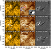 |
Fig. 1. Temporal evolution on 14 March 2015 in SDO-AIA 171 Å (left column), 193 Å (central column), and in GONG Hα (right column). In panel (b), the images are overlaid with the HMI magnetogram of the AR. In the same panel, an inset shows a detail of the HMI magnetogram around the AR central bipole. It consists of a bipole with a positive polarity (P, in red) surrounded by negative polarities (N, in dark blue). In panel (c), the image is shown in Hα with a large F filament studied in this work and a small f filament in the AR. The f eruption is related to the first jet on this day. In panels (d) and (e), jet1 appears as a bright structure, marked with the white arrow. It is visible in the AIA pass bands, but not in the Hα; see panel (f). After the impact of the jet1, the F filament splits into two segments. In the AIA channels ((g) and (h)), both parts can be seen, but it is much clearer in Hα (i). The segments are labelled RF and DF. The DF segment detaches from the body of the initial filament and is ejected up and towards the south. This segment will erupt the next day. In panel (h), inset, a detail of DF is shown. This reveals the structure of the filament in the form of threads oriented along the NW direction. An animation of this figure is available online. |
The filament is very wide in the GONG Hα images in the southern hemisphere and also seems to be of sinistral magnetic class due to the appearance of the barbs (regularly spaced feet of the filament) towards the left. As the GONG filter has a large bandpass, this suggests that the filament can be seen in different wavelengths in the Hα wings indicating perturbations with blueshifts and redshifts, enlarging the line profiles (Schmieder et al. 1985). The images in 171 Å and 193 Å (Figs. 1a and 1b) show the absorbing filament and a larger dimmed band forming the sigmoid-shaped filament channel. In addition to the large filament, there is also a small narrow AR filament close to the positive spot P labelled with f in Fig. 1c. This small filament is related to the first jet that we describe in the following.
This AR showed a lot of activity with B- and C-class flares, as shown by the GOES data given in Fig. 2. The relevant events for the current study are a C2.6 flare taking place at 11:44 UT (green box on the left in the figure), and C2.4 and C9.2 flares on March 15 (green box on the right) described in Sect. 3.2. This activity corresponds to the first and second phases of the event.
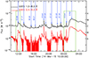 |
Fig. 2. Succession of flares from AR 12297 on March 14–15 2015 registered by GOES. The GOES classification of flares measures the peak flux in the 1–8 Å range (black curve) and in the 0.5–4 Å range (red curve). The vertical blue arrows show the recurring solar flares from AR 12297 for the period from March 14 10:00 UT until March 15 6:00 UT. The two green boxes delimit the two flare events we are interested in. The first event contains one C2.6 flare, whereas the second includes two flares, of class C2.4 and C9.2, respectively. Jet1 occurs almost simultaneously after the C2.6 flare on day 14, whereas jet2 erupts just after flare C2.4 on day 15. |
Consecutively after the small C2.6 flare at 11:44 UT, there is the ejection of a jet hereafter referred to as jet1. This jet is clearly visible in Figs. 1d and 1e. Both images show the well-developed jet ten minutes after ejection. Jet1 appears to be launched from the sunspot’s penumbra. This jet moves to the south-west, and some threads are detached and reconnected with field lines of the filaments (Figs. 1d and e). In Sect. 4, the jet velocity is estimated to be 151 km s−1 using the time-distance technique. This activity corresponds to the double peak in Fig. 2 around 12:00 UT marked with the green box on the left. The Hα images show a bright sigmoid, which is the signature of a flare (Fig. 1f). The flare that will eventually produce jet1 could be related to the eruption of the small filament labelled f in panel (c) that has disappeared in panel (f). This eruption produced a slow CME (350 km s−1), as observed by the LASCO coronagraph (Liu et al. 2015; Wang et al. 2016a).
The interaction of jet1 and filament F results in the detachment of a large portion of the filament from its main body (see Figs. 1g–i). Henceforth, we call the two resulting pieces the remaining filament (RF) and the detached filament (DF; called F1 in Chandra et al. 2017) as marked in panel 1i. The DF can also be seen in 171 Å and 193 Å, where its thread-like structure can be discerned. This DF segment changes its position until it reaches a new equilibrium. It remains in more or less the same position until the next day when another jet triggers its eruption.
3.2. Second phase on March 15
Figure 3 shows the temporal evolution of the second phase, which took place on March 15. An eruption occurred that is considered to be the trigger for the great St Patrick’s Day geomagnetic storm on March 17 (see Sect. 1). For a full and detailed description of the mechanisms that trigger this eruption, we invite the reader to consult Bamba et al. (2019). Figure 2 (green rectangle on the right) shows two peaks, one of them associated with a C2.4 flare at 00:34 UT and the other corresponding to a long-duration C9.2 flare starting at 01:15 UT and lasting until 05:00 UT with a secondary peak around 04:20 UT. Simultaneously with the C2.6 flare at 00:34 UT, a small filament or jet (hereafter referred to as jet2) escapes and hits the large filament in the south of the region. We see the absorbing plasma and parallel bright strands in the AIA 171, 193 Å filters (Figs. 3a and 3b) and cool material in Hα (Fig. 3c), suggesting that it is a surge with a small filament at the base. Jet2 appears to impact RF and also precipitate the eruption of DF. Around 00:45 UT, DF starts to rise with increasing speed. In Fig. 3, it can be seen that DF has moved and is slightly more separated from RF. In panels 3d–3f, we have marked the position of DF with a white arrow in the three wavebands. In 193 Å, DF is clearly visible; however, in 171 Å and Hα it is more difficult to identify it. In Hα, we increased the contrast of the image for better visualisation. It can be seen that DF has already started to rise slowly at first, but considerably faster shortly afterwards. Chandra et al. (2017) made a detailed analysis of the DF eruption and estimated that the projected rise velocity is 70 km s−1 in the last phase of the eruption.
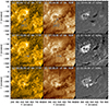 |
Fig. 3. Temporal evolution on 15 March 2015; similar to Fig. 1. Panels (a) and (b) show the jet2 marked by a white arrow. In both AIA panels, the plasma is seen by absorption. A dark structure is also seen in panel (c). In panel (c), the two filament segments are seen. Jet2 hits DF and triggers its eruption. In the middle row, DF (white arrow) is slowly rising. In the last column, the fulguration associated with the DF eruption is occurring. In (g) and (h), the postflare loops are visible. In panel (i), chromospheric brightenings are also seen. These brightenings form two ribbons, one north and one south, although the shape is not well defined. It is clearer in later times and we recommended consulting the animation accompanying this figure. In panel (i), the RF segment has an elongated shape because it is pushed in a NW direction. An animation of this figure is available online. |
The C9.1 flare starts at around 1:10 UT in the AR, and two ribbons extend east-west. In panels 3d–3f, the bright structures are visible, but, in the following panels 3g–3i, the ribbons are clearer. Brightening is also observed in 171 Å in the whole region around the AR and also in the RF filament (as we see in Fig. 4). This is considered in detail in Sect. 5. When the flare reaches its maximum at 2:00 UT (see Fig. 2), post-flare loops appear and are seen in panels 3g and 3h.
 |
Fig. 4. Temporal evolution of DF eruption and the triggering of the oscillations in the RF segment in 171 Å data. In panel (a), the absorbing plasma of the RF and DF segments shown in the figure is visible. In the same panel, the white box delimits the area where jet2 is located. In panel (b), DF jet2 has already impacted DF, and this segment is already erupting. Jet2 also impacts RF, producing a slight brightening in a small area on the RF spine (blue arrow). During the eruption of DF, it seems that changes also occur in RF, such as the appearance of a protrusion on its west side (green arrow). This same protrusion (green arrow) becomes bright shortly afterwards. In panel (d), within the white box, a lot of brightening can be seen on RF. In the next panels, from (e) to (h), the brightenings are massive over the whole structure, and in (i) loops can be seen in the NW area (green arrow) outlining a kind of flux rope structure. An animation of this figure is available online. |
4. Time-distance analysis
In this section, we study the oscillations and jets that occur on 14 and 15 March. Our aim is to qualify and quantify the characteristics of the oscillations and put them in the context of the activity of the region.
4.1. First phase
The triggering is related to the C2.6 flare at 11:44UT on March 14, the first jet (jet1), and the detachment of part of the filament (DF). As we describe in Sect. 3, jet1 splits the large F-filament into two parts, which are labelled RF and DF. The DF segment changes its position until it reaches a new equilibrium (Chandra et al. 2017). This results in oscillations in both segments. The movement of DF to a new position probably shakes the plasma of the prominence and contributes to the oscillation.
To study the oscillations of RF and DF, we used the time-distance technique with the 171 Å data. Figure 5 shows one frame of the AIA 171 Å data where jet1 appears as a bright structure. Overplotted on the image are the white contours of the artificial slits used to extract the intensity as a function of time. To define the curved slit in the images, we tracked the path of the oscillations by visual inspection. We trace the oscillation motion of the filament segment we are interested in and include the trajectory of the jet. With the artificial slits S1 and S2, we track the oscillations on DF and RF, respectively. We note that DF is not yet under S1 at the instant shown in the figure. However, after the jet, DF moves to a new position under S1, and we can follow its oscillation. It is unclear how jet1 triggers the oscillation in DF as the jet does not appear to flow along the field lines where DF is located. We think that the structural changes that occur after the jet1 ejection cause the oscillation of the cold plasma in DF. As we see in Fig. 5, most of the jet flows are oriented in the SW direction, and some are moving to the NW, roughly following the direction of S2. The NW-bound flows move along S2 until they interact with the RF segment. To get a better view of the NW-bound flows, we have enlarged the area marked in the white box and shown it in the inset of Fig. 5; the bright elongated structure in 171 Å is clearly visible in it. In addition, part of the jet1 flows move towards RF, thus producing its oscillation.
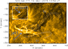 |
Fig. 5. AIA 171 Å image showing the artificial slits S1 and S2 used to study the oscillations on DF and RF, respectively. S1 has a width of 4 arcsecs, whereas S2 has a width of 10 arcsecs. The figure shows jet1 (white arrow) interacting with the filament. This jet will split the filament in two: DF and RF (see Fig. 1). However, this shows an early stage, and DF has not yet moved to its new position under the S1 slit. Part of the jet1 flows are directed in a NW direction along S2. The inset shows the white box area enlarged to show the details of the NW-bound jet. |
Figure 6 shows the resulting time-distance diagrams for both the S1 and S2 slits. In diagram 6a, we see that the jet1 perturbation reaches S1 around 12:00 UT as a collection of bright features. Between 13:00 and 14:00 UT, we can discern the apparently oscillatory motion of dark features. They are out of phase and it is difficult to adjust any clear oscillation to them. However, from 14:00 UT onwards the oscillatory motion is clear and can be seen until after 16.00 UT. In that time range, we can follow the oscillation and fit a damped sinusoidal curve using Eq. (1). Table 1 shows all the best-fit parameters of Eq. (1) for all the oscillations studied in this work. In Sect. 4.3, the results obtained with prominence seismology are presented and discussed. In Fig. 1h, an inset is plotted showing the enlarged area delimited by the white box over the spine of the filament. In this inset, we observe elongated structures probably aligned with the magnetic field, forming an angle with the spine of the filament. These appear to be individual cool threads, or clusters thereof, seen in absorption. In the observed oscillations the threads move along their axes, so we can assume that the oscillations are longitudinal. The perturbation probably also induces transverse oscillations, but we were not able to detect them. Correspondingly, Fig. 6b shows the time-distance diagram of S2. In this case, we can identify the triggering, which is the NW-bound flows of jet1. The interaction resembles the one described in Joshi et al. (2023), which fits the Luna & Moreno-Insertis (2021) model for the jet-prominence interaction. With a single slit, we can track the jet and the oscillation. The jet starts at 11:44 UT and in the diagram it appears as a collection of straight bright features. These have an inclination that depends on the propagation speed. We determine the jet velocity by fitting a straight line (red dashed line) over these brightenings. We conclude that the jet1 flows move along S2 with a velocity of 151 km s−1. From the diagram, we also appreciate that jet1 reaches the filament at the slit position s = 180 arcsec a few minutes after the jet1 ejection, thereby triggering the oscillation. Part of the hot jet flows continue propagating along S2, as seen in the bright straight lines above s = 180 arcsecs in the diagram. Between 12:00 and 13:30 UT, we can clearly identify the oscillation. In contrast, from 13:30 to 14:30 UT, it is less clear, and after 14:30 UT no dark thread oscillation is visible. We have fitted a damped sinusoidal as in Eq. 1 to the oscillatory pattern (white dashed line) obtaining the parameter values shown in Table 1.
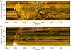 |
Fig. 6. Time-distance diagrams of March 14 constructed with the artificial slits shown in Fig. 5. In panel (a), the diagram for S1 over DF is shown, and in panel (b), the diagram in S2 over RF is shown both panels in AIA 171Å. In this pass band, the prominence plasma appears in absorption as dark bands. The white dashed line shows the oscillation fit using Eq. (1). The best-fit parameters of the oscillation are shown over both panels. In panel (b), the fit is also shown by plotting jet1 with a red dashed line. This gives the jet propagation velocity shown in the panel. |
Best-fit and seismology parameters of the three oscillations reported in this work.
4.2. Second phase
In this section, we study the characteristics of the oscillations that occur the next day. The trigger of the oscillations will be analysed in a separate section (Sect. 5). On March 15, the DF segment erupts at 01:15 UT. This eruption produces a huge LALO in the RF segment. The same eruption is also responsible for the St. Patrick’s Day geomagnetic storm on Earth on March 17. Figure 7 shows the RF filament during the triggering phase. Bright loops outlining the structure of the filament channel are visible. Dark strands are seen along with the bright plasma. The dark strands will be part of the prominence that is displaced towards the northwest end of the filament channel. In the figure, we have drawn the two slits used in the second phase. S3 was used to study the jet produced in the AR and S4 was used to track the oscillation.
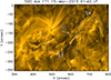 |
Fig. 7. AIA 171 Å image showing filament on 15 March, similarly to Fig. 5. The artificial slits S3 and S4 are shown. S3 is used to study the propagation of jet2, while S4 is used to study the oscillations of the RF segment. Both slits have a width of 10 arcsecs. |
Figure 8 shows the time-distance diagram constructed with S4. This diagram shows that the triggering of the oscillation occurs approximately between 01:10 and 02:10 UT. It is interesting to note that the impulse occurs over quite a long time frame and is not an instantaneous process in contrast with the case produced by jet 1 shown in Fig. 6b. After 02:10 UT, the oscillation of the cold plasma that appears in absorption is already visible. The oscillation is very clear and extends beyond the time interval considered in the figure. It can be seen that several threads move in phase during the first cycles of the oscillation but end up losing global coherence at the end of the diagram. We used the technique discussed in Sect. 2 to track the movement of the filament. Fitting this data with Eq. (1), we obtain the curve shown as a dashed white line. The best-fit parameters of the oscillation are given in Table 1. The amplitude of the velocity is quite large, and considering that the whole prominence is involved in the oscillation the energy must be enormous. In Sect. 6, considerations regarding the energy associated with these oscillations are presented.
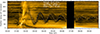 |
Fig. 8. Similar to Fig. 6, but with the time-distance diagram in 171 Å along slit S4 shown. The oscillation best-fit parameters are shown in the figure with the white dashed line. Bright structures are seen between 01:10 and 02:10 UT, which is the impulsive phase when the oscillation is triggered. After 2:10 UT, the absorbing plasma in the filament moves periodically around y = 120 arcsecs. Between 6:30 and 7:20 UT, there is a gap with no SDO data. |
4.3. Seismological analysis
We applied a seismological analysis of the studied oscillations as described in Sect. 2. With the oscillation periods (see Table 1), we obtain information on the radius of curvature of the magnetic dips, R, as well as the value of the field strength, B. The periods are similar for the three cases and range from 62 to 72 minutes. With Eq. (2), we then obtain radii of curvature for the three events that range from 111 to 159 Mm. We see that the RF oscillations of March 14 yield a radius of 111 Mm. By the next day, the radius of curvature of RF has increased to 159 Mm. The magnetic field strength has also increased a little, namely from 19 to 22 Gauss. The reason for the changes may be that we are analysing different field lines on each day; another option is that this difference may be associated with the structural changes that occur in the filament during the eruption on March 15. However, further study of the oscillations would be necessary to confirm which option is most likely to be correct. The radius of curvature obtained for the DF segment is 143 Mm (Table 1, first line). Interestingly, this portion that has partially erupted has a radius of curvature similar to that of the remaining part. This may indicate that the dips of this detached segment do not change considerably during this process.
5. Trigger of the huge oscillation on March 15
The main motivation of this work is to understand the triggering of the huge oscillation on March 15. In this section, we show the observational evidence that can explain how the filament is set into motion in detail. As discussed in Sects. 3.2 and 4.2, the oscillation occurs following the C2.4 flare and jet2 at 00:34 UT.
Figure 9 shows the time-distance diagram for S3 following the jet2 flows in 171 Å, 131 Å, and 94 Å. There are two vertical grey lines representing the times when the first flare C2.4 (left) occurs and the second flare C9.2 (right) starts. We measured the propagation speed of jet2 in the three pass bands. Around 00:34 UT, the jet starts to propagate along S3 with a speed above 200 km s−1 in all the channels. As we can see, the measured velocity depends on the AIA channel. However, this does not necessarily imply a dependence of speed on temperature, as the method of measuring inclination is itself quite uncertain. We can give an estimate of the jet speed as the average 235 km s−1 of the three channels. At 00:50 UT, the flow becomes quite diffuse and part of the ejected plasma falls back down again (Fig. 9a). This is a parabolic movement that can be clearly seen in the 171 Å and 131 Å diagrams, but not in the 94 Å one. At around 01:20 UT, bright structures appear in the filament, such as those shown in Fig. 8. These brightenings are very clear in 171 Å and 131 Å, while in 94 Å they are more diffuse. They are associated with the impulsive phase in which the oscillation is triggered. It can be seen that jet2 and the triggering are well separated in time, in contrast to the effect of jet1 shown in Fig. 6b. The diagram also shows the filament as a dark horizontal band centred at y = 150 arcsecs before 01:20 UT. It is difficult to determine the exact moment when jet2 reaches the filament. However, we can estimate that it could be between 00:45 and 01:00 UT. The first time corresponds to the intersection of the prolongation of the red dashed curve with the black filament at y = 150 arcsecs. The second is the time when the jet visually reaches RF, as we show later in the paper. This indicates that there is a delay of some 20 minutes between the arrival of the jet2 flows and the impulsive phase. As discussed in Sect. 3.2, between 00:34 UT and the impulsive phase of the oscillation the DF segment erupts and the C9.2 flare occurs (right vertical grey line in Fig. 9), starting at 1:15 UT and peaking at around 02:00 UT. This coincides with the impulsive phase of the oscillation. With this figure, it is clear that jet2 is related to the first flare, but it is when the second flare starts that the brightenings on the filament are visible. In channels 131 Å and 94 Å – Figs. 9b and 9c, respectively- no features are seen flowing along the slit. However, the plasma below y = 150 arcsecs (i.e. to the south-east of the filament) has strong emission after the second flare. This suggests a heating of this area. In all the panels, between the two vertical lines (between the two flares) the filament already starts to move slowly; that is, the dark band moves along S3. This could mean that the whole structure starts to change during the DR eruption.
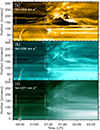 |
Fig. 9. Time-distance diagram for jet2 along the artificial slit S3 (Fig. 7) in 171 Å (panel a), 131 Å (panel b), and 94 Å (panel c). In all the panels, the two vertical grey lines mark the times of the first C2.4 flare at 00:34UT and the second C9.2 flare starting at 01:15UT. Also in the three panels, by fitting a straight line (red dashed line) we estimate the speed of the jet2 flows on each pass band. The jet2 propagation velocities are shown in each panel. The average value for all three pass bands is 235 km s−1. |
Figure 4 shows the temporal evolution in the AIA 171 Å pass band. In panel 4a, we can distinguish both segments RF and DF; jet2 can also be identified in the left of the panel and is marked with a white box. We can see that it is composed of bright hot plasma, but also of dark plasma seen in absorption. These flows continue propagating forming arched curves in the direction of the RF. As we have mentioned in the previous paragraph part of the plasma moves back to the origin of the jet, but part also interacts with the filament. In panel 4b, we mark a bright region over the RF, which is the region where the flows reach the prominence, with a blue arrow. There is no evidence of oscillation triggering in that region directly following the impact of the jet. After jet2, the DF appears to start to rise slowly and roll-unroll around itself, as reported by Wang et al. (2016a). It seems that the structure of the RF prominence changes during the DF’s rise (see animation in Fig. 4). The cold plasma can be seen to move slowly. A protrusion marked with a green arrow also appears in 4b. A few minutes later, this protrusion becomes bright, indicating that some heating is occurring in it; in fact, this seems to be the first RF region where the triggering starts (see panel 4c; green arrow), and it is worth remarking that this region is relatively far from the impact of jet2 on the RF (blue arrow on Fig. 4b). In the next panel, (d), the brightening starts to appear in the south of the RF, as marked with a white square. In panel (e), the brightenings are widespread, and in panel (f) they are clearly apparent in the entire RF. In these images, the bright structures can be seen to have a fibrillar structure; these fibrils are probably the filament threads, which have become bright by some mechanism during this phase. We come back to these brightenings at the end of this section. In the following panels, 4g–4i, the bright structures can still be seen delineating the twisted structure of the magnetic field in the filament channel. This is especially clear in panel 4i, where they are marked with a green arrow. This sequence of images clearly shows that after the fading of the jet2 flows, the triggering continues for more than an hour. This excludes jet2 as the direct cause of the oscillation. Still, jet2 seems to be involved in some way, possibly activating other processes that ultimately trigger the oscillation.
Looking again at Fig. 4 and the associated movie, we cannot identify any plasma emitting in the 171 Å pass band clearly pushing the filament’s cold plasma. To determine whether there is hotter plasma pushing in, we studied hotter lines such as 131 Å and 94 Å. Figure 10 shows twice during the triggering phase. We also plot 171 Å images (top panel row) to give them context, as the RF environment is better visualised in them. In these images, we employ the WOW technique (see Sect. 2) to enhance the visualisation of the coronal structures. On the left side of the images in the hotter channels, we can clearly see the bright post-flare loops (Figs. 10c–10f). In the images, the northern ribbon can be seen as a bright thin line where these loops are rooted. In fact, this ribbon can be seen in all three channels shown in the figure. However, the southern ribbon is less clear, and in 131 Å and 94 Å it is hidden behind the postflare loops. In the east of this whole structure, the post-flare loops form an arcade connecting the two north and south ribbons; however, towards the west at about x = 500 arcsecs, the arcade is reoriented and the north foot becomes connected to the magnetic structure of the filament. This plasma traces a twisted field line from the northern ribbon to the prominence. These hot structures are visible in the 131 Å and 94 Å channels for more than ten minutes, although different tubes appear to be illuminated, as can be checked by comparing the two times shown in Fig. 10. The other AIA wavelengths have been analysed, and these structures could not be identified.
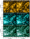 |
Fig. 10. Plot showing two moments during triggering of huge oscillation in AIA 171 Å, 131 Å, and 94 Å. The images have been processed using the WOW technique described in Sect. 2. The left column shows the region at 1:33 UT. In 171 Å (a) the structures already discussed in Fig. 4 are visible. In 131 Å (c), however, the post-flare loops around the flare are visible, as well as bright tubes in this pass band from the flare area to the filament. The white arrows indicate the region where the bright tubes appear in 131 Å and 94Å. These appear to trace a twisted field line reminiscent of a magnetic rope. Similar structures can be seen in 94 Å (e). Later, in the right column, the structure has evolved, but the bright tubes connecting to the prominence at both wavelengths are still clear. We note that these bright tubes are not visible in 171 Å. In 171 Å, the white arrows show the areas where the tubes appear in 131 Å and 94 Å. An animation of this figure is available online. |
The analysis of the AIA images indicates that there are tubes connecting the flare zone to the filament that may contain very hot plasma. Figure 11 shows an analysis of the temperature of one of those flux tubes. In panel 11a, we show a small box where we analyse the temperature distribution at 1:33 UT using the DEM inversion technique proposed by Hannah & Kontar (2012). This DEM method effectively constrains the emission-measure (EM) values using the AIA-SDO observations in six wavelength channels (94, 131, 171, 193, 211, and 335 Å). Here, we used a temperature range from log T(K) = 5.5–7 with 15 different bins of width Δlog T = 0.1. It can be seen (panel b) that there are two peaks in the temperature distribution, one around 0.6MK and the other at 2MK. However, the EM distribution increases for higher temperatures, with the maximum EM in the figure being reached at T = 10 MK, where the technique loses its validity. This distribution reveals the existence of very hot plasma in these tubes. We are cautious with this statement as recent studies show that the DEM inversion technique overestimates the presence of hot plasma (T > 2.5 MK) by a factor of three to 15 (Athiray & Winebarger 2024). The DEM analysis allows for the estimation of electron density and gas pressure (see, e.g. Saqri et al. 2020; Paraschiv et al. 2022, among others). However, in our case, the EM may well be overestimated in the hotter part of the range shown in Fig. 11b, which would lead to an erroneous calculation of these parameters. In addition, there are other sources of uncertainty. The cited papers assume that the emitting plasma is cylindrical and that the amount of plasma emitted along the line of sight (LOS) coincides with the thickness of the tube seen in the images. In our case, we see a well-defined tube, but there is probably much more hot plasma along the LOS. Furthermore, the filling factor, which cannot be measured, contributes to the uncertainty. This makes the DEM method unreliable for a quantitative determination of density and pressure. Despite all this, the EM indicates the presence of very hot plasma (at least 10 MK), as suggested by the intensities in the different pass bands. In panel (c), we show the temporal sequence of the average intensity for all AIA EUV channels within the small box area considered. From 1:27 to 1:38 UT, the intensity in 94 and 131 Å increases, whereas it decreases for the rest of the AIA channels. This is in line with the existence of very hot plasma. According to the temperature response functions for channels 131 Å and 94 Å, both have two emission peaks. In both cases, the first one is below 2MK, whereas the second one is above 6.3MK. If the temperature of the plasma were below 2MK, one would expect emission in channels such as 171 Å. However, clear emission is only observed in 131 Å and 94 Å. These two lines only emit in isolation at around 10MK, which indicates that the plasma in these tubes must have a high temperature. After 1:38 UT, the bright tube that crosses the small box is no longer visible. However, other bright tubes appear, as can be seen in Fig. 10d. This indicates that heating is occurring in different field lines as the flare evolves.
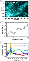 |
Fig. 11. Temperature analysis of small region shown in the box in panel (a). In panel (b), the temperature analysis of that area using DEM is shown. In panel (c), the average intensity in the same area of all AIA wavebands is shown. The colours used are inspired by the respective AIA channel palette. |
During the impulsive phase, the prominence plasma becomes brighter in 171 Å (see Fig. 4) and the 131 Å and 94 Å bands, as seen in Figs. 10c and 10e. These brightenings may be due to the interaction of the hot plasma of the flare with the cold plasma of the prominence. Figure 12 shows a detail of the observed fibrilar structures in a region at the southern end of the prominence (marked by the white box in Fig. 4d). In 171 Å (Fig. 12a), the green arrows point to an area where fibrilar structures are visible. They are also visible, and have a similar shape, in 131 Å (panel b). In 94 Å (panel c), a very faint structure is discernible in those positions, although it is difficult to associate it with fibrils.
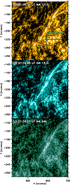 |
Fig. 12. Details of brightening observed in prominence in AIA 171 Å, 131 Å, and 94 Å pass bands. The region corresponds to the white box in Fig. 4d. The green arrows show the bright fibril-like structures at the southern edge of the prominence. |
Based on this figure and the preceding ones, it is evident that the brightenings predominantly appear in the southern section of the filament, which is situated closer to the flare. The threads exhibit increased luminosity towards their ends, where they are closest to the flare and experience the impact of the hot plasma.
6. Some estimates
This analysis suggests a possible mechanism for the triggering of the huge oscillation of the RF segment. The hot plasma is only on one side of the filament, in the SE, and is only visible during the impulsive phase of the oscillation. This hot plasma increases the pressure on this side of the filament, pushing the filament to the NW and initiating the oscillation. This hot plasma is possibly chromospheric plasma evaporated in the ribbons in the flare zone. Due to the energy and mass supply of the flare, we think that the pressure and temperature remain high during the impulsive phase.
We developed a relatively simple model (see Appendix A) that may represent the temperature increase at one leg due to the energisation process that eventually produces the excitation of the large oscillation. Using this model, we obtained some estimates associated with the pressure increment and the subsequent relaxation. Although a detailed analysis of the process requires the numerical solution of the MHD equations that include the effects of conduction, radiation, and heating, together with a model of the chromosphere, we investigated the use of a simplified model that allows us to obtain some analytical expressions for the displacement of the threads and their maximum amplitude of oscillation.
The model consists of a flux tube of length L with a central part of curvature radius R. Details of the geometry are given in Appendix A. We consider a thread of length lt and density ρt. The rest of the tube outside the thread has a density ρ0. The thread is initially located at L/2, which represents the bottom part of the dip. Due to an overpressure at the left leg (from p0 to pmax), the thread achieves a new equilibrium position at L/2 + δse. The thread displaces to the right side and upwards as it moves along the curved dip. According to our linear calculations, this displacement should be of the order of (see Eq. (A.8))
where γ = 5/3. The numerator of this equation shows that the displacement of the thread to a new equilibrium location is linearly proportional to the pressure increment.
Once the thread is in its new equilibrium position, we assume that the overpressure at the leg suddenly disappears, going from pmax to p0. Therefore, the thread falls back to the bottom of the dip at L/2 and oscillates around this position with an amplitude δse, because it has gained some extra energy due to the initial rise in pressure. Using energy conservation of the system composed of the dense thread and the evacuated parts, the maximum velocity of the oscillating thread is found to be (see Eq. (A.14))

where δse is given by Eq. (4). We aim to compare these values for the thread displacement and velocity with the ones derived from the observations to assess the scenario of the oscillation induced by an initial overpressure followed by the relaxation.
From the analysis of the AIA images in 171 Å and 131 Å, we estimate that L ≈ 620 arcsecs and that lt is between 10 and 20 arcsecs. We note that those values are the plane of the sky projections. Furthermore, from the previous section, we can see that the thermal increment in the left foot can exceed 10 MK. Thus, we assume that pmax/p0 ∼ 10, where the initial temperature is considered to be 1 MK. The radius of curvature is taken as the value obtained from the seismological estimation of Table 1, R = 159 Mm. With these numbers and from Eq. (4) we estimate a range of values for δse = 75 − 38 Mm, where the first value corresponds to lt = 10 and the second to 20 Mm. This range of values comprises the value obtained in the oscillation amplitude 57 ± 15 Mm. Similarly, from Eq. (5) we obtain a v = 98 − 51 km s−1 range. The value obtained with the oscillation fit is 73 ± 16 km s−1, which is also in agreement with the estimation. The values of the rough estimates indicate that the proposed mechanism of temperature and pressure increase on one side of the filament can explain the oscillations quantitatively.
This simple model provides also an estimate of the energy released by the flare. The value obtained is a lower limit since only part of the energy released reaches the filament. The flare pushes the filament upwards along the dipped magnetic field lines, converting some of its energy into kinetic and potential energy of the threads. However, the flare also increases the internal energy of the evacuated regions on either side of the flux tube. Additionally, the pressure within the flux tube rises to a peak value (pmax), and the region right of the filament is compressed. By accounting for these contributions, we arrive at Eq. (A.16). Using some estimates and typical values for the parameters, such as pmax/p0 ≈ 10, ρth/ρ0 = 100, p0 = 1 dyne cm−2, and ρ0/mp = 108 cm−3 (where mp is the proton mass), we can estimate the flare energy:
Here, we considered a filament length (lth) between 10 and 20 arcsec. However, all these values yield identical orders of magnitude. For a typical prominence mass (Mprom) of 1012 − 1015 g (as cited in Labrosse et al. 2010), the estimated flare energy falls within the range of 1028 − 1031 erg. The obtained range is broad, encompassing values similar to X-class flare energies (see reviews by Benz 2008; Shibata & Magara 2011). This indicates that we are overestimating this energy. Our analysis assumed all the mass moves at the maximum velocity; however, only a fraction likely reaches this speed. An in-depth study with more realistic models and numerical simulations is needed.
7. Discussion and conclusions
In this work, we studied the oscillations accompanying the two-step filament eruption that occurred on 14–15 March 2015. This event is known as the St Patrick’s event of 2015 because the part of the filament that erupted produced a CME and a large geomagnetic storm on Earth on March 17. The eruption occurred in two phases and was well studied by Chandra et al. (2017). In the first phase on March 14, a small flare and an associated jet, jet1, produced the detachment of part of the filament. Both the detached filament (DF) and the remaining filament (RF) segments oscillate. It is unclear from the observations what the triggering agent of the DF oscillations was. However, during this first phase, the DF rises from its original location to a new metastable position (Chandra et al. 2017). This change in position is likely to perturb the DF plasma, causing its longitudinal oscillation. The DF segment moves with a longitudinal oscillation of period og 69 ± 3 minutes and characteristic damping time of 297 ± 369 minutes. We applied seismological techniques to obtain a radius of curvature of the dips of the filament of 143 ± 15 Mm and a magnetic field strength of 21 ± 11 G. In the case of the RF segment, part of the jet1 flows reach the filament and trigger its oscillation. From the time-distance analysis, we can see that the jet1 flows propagate with a velocity of 151 km s−1 reaching the filament and producing a displacement of the plasma of the prominence. Jet1 and the displacement of the prominence are consecutive, so we conclude that it is the impact of the jet flows that is responsible for the initiation of the oscillation. The interaction resembles the one described in Joshi et al. (2023), which fits the Luna & Moreno-Insertis (2021) model for the jet-prominence interaction. In this case, only a small part of the filament oscillates with a period of 62 ± 2 minutes, a damping time of 281 ± 166 minutes, and a velocity amplitude of 33 ± 3 km s−1, which is also a LALO. Using seismological techniques, we infer a radius of curvature of the dipped field lines of 111 ± 8 Mm and a magnetic field strength of 19 ± 10 G.
In the second phase on March 15, another small flare is produced and an associated jet is launched (i.e. jet2 ). This is followed by a huge oscillation in the RF segment. The oscillation is a LALO with a period of 72 ± 2 minutes, a damping time of 196 ± 71 minutes, and a velocity amplitude of 73 ± 16 km s−1. With these data, we estimate the radius of curvature to be 159 ± 11 Mm and the field to be 22 ± 11 G. We investigated the possible triggering of this oscillation. Following a detailed analysis, we find that the impact of jet2 and the triggering of the huge oscillation are not truly consecutive events. In addition, jet2 impacts a small RF area even though the whole filament is set to oscillate. This leads us to discard the impact of the jet2 flows as the triggering of the LAOs in the RF. Using the SDO-AIA images, we can see that after jet2 there are structural changes in the filament probably associated with the DF eruption. Around 01:08UT, we start to see brightenings in the filament that will later become massively present throughout the entire RF. The time-distance analysis shows that the appearance of these brightenings is simultaneous with the triggering stage. This phase lasts for about an hour, after which point the RF is seen to oscillate. We analysed the AIA data at 171 Å, 94 Å, and 131 Å and do not observe plasma flows moving from the AR region to the filament. This indicates that it is not a jet-type triggering where the plasmas emanating from the reconnection are pushing the filament cold plasma. However, images at 131 Å and 94 Å show flux tubes connecting the prominence to the flare region (Fig. 10). This indicates that the same mechanisms that heat the post-flare loops also heat the nearby filament channel feet. The bright tubes trace a complete flux rope with the presence of a dip where the prominence is located. This causes an increase in the pressure on the SE side of the filament, which pushes the filament towards the NW. This heating and pressure increase is not visible in the AIA channels. This heating leads to the evaporation of the chromospheric plasma and fills the tubes with hot, dense plasma. It is at this point that the tubes are visible, which is after the first moments of triggering. For this reason, we do not see any agent pushing the filament, as it is initially not visible in the AIA channels. Other evidence of this possible heating is the threads of the filament becoming bright in 171 Å and 131 Å. Initially, fibril-like structures appear, which we think are the ends of the threads that are heated by this hot plasma. These structures are similar to those seen in the ribbon, which must be associated with the heating of the chromospheric material by the flare.
We infer that the triggering of the large oscillation observed on 15 March 2015 might be linked to plasma energisation during the flare. However, the specific mechanism responsible for transferring flare energy to the filament remains elusive. The two structures, while seemingly independent, exhibit the presence of very hot magnetic tubes connecting them. This suggests a magnetic connection between the filament channel and a region near the flare. It is plausible that heated plasma from the flare exerts a force on the filament, initiating the oscillation. Three potential mechanisms can be envisioned: (1) energy transfer from the flare to the filament channel at their foot points; (2) inclination of the whole filament structure; or (3) reconnection of the erupting DF filament with the remaining channel. In the first scenario, the foot points of the post-flare arcade would be situated close to those of the filament channel. This expectation arises from the fact that the DF belongs to the same channel. According to the CSHKP model (Carmichael 1964; Sturrock 1966; Hirayama 1974; Kopp & Pneuman 1976), the footpoints of post-flare loops experience heating due to particle and heat flows that trigger chromospheric evaporation. Recent studies by Druett et al. (2023) and Druett et al. (2024), based on 2.5D flare simulations, demonstrate that evaporation flows can potentially leak out of the post-flare arcade into surrounding regions. In Fig. 6 from Druett et al. (2023), the authors show that the evaporation precedes the arrival of the electron beams, in what they call pre-heated loops. Figure 14 from Druett et al. (2024) shows 1D cuts along a field line as functions of time. They show that the evaporation starts approximately ten seconds before that line is reconnected. The authors suggest that this may be due to the compressive heating of neighbouring flux tubes or heat diffusion. Notably, evaporation precedes electron beams. This implies that plasma evaporated as a consequence of the flare might escape the arcade and enter the filament channel through its neighbouring foot points. This influx of high-pressure, high-temperature plasma could then push the prominence, triggering the large-amplitude oscillation. However, this evaporation appears to occur only on field lines just ahead of the ribbon front and shortly after reconnection, effectively bringing the evaporation just seconds ahead of the reconnection. In the second scenario, the DF eruption produces the elevation of the south-east zone of the RF filament channel resulting in the inclination of the structure. This causes the cold plasma to slide down along the channel to a lower position, which would initiate oscillation around a new equilibrium position. However, this scenario cannot explain the massive brightenings as seen in Fig. 4 or the bright fingers shown in Fig. 12, which are both associated with a temperature increase.
To illustrate the third scenario, we present a schematic diagram in Fig. 13 on March 15, when the DF and RF segments had already separated. We note that the structure’s size has been intentionally exaggerated relatively to the size of the Sun. This allows for a better perspective, and by including the limb we give information about the height of the different parts of the structure. In panel 13a, two field lines (black lines) depict the filament channel located above the polarity inversion line (PIL) via a dashed line on the solar surface. The line with feet at A and B illustrates the field hosting the RF filament segment, while the line with feet at C and D hosts DF. The RF and DF segments are represented by two black ellipsoids, aligned with the field lines. Figure 13b shows the eruption of DF. We note that the field line foot points C and D are no longer shown to simplify the figure. According to the standard CSHKP model, a reconnection zone, represented by an orange band in panel (b), forms beneath the erupting structure within a current sheet. The core of the coronal mass ejection (CME) is represented by a green circle and contains part of the DF mass. A circular blue line represents the erupting flux rope. The green curve represents a newly reconnected field line in the current layer, connecting points E and F. This line contracts due to magnetic tension, transforming into the red line. Both lines depict two stages of the same field line evolution and share the same foot points. During contraction, the reconnected line (red) intersects with the filament channel lines (black), triggering another reconnection event. This reconnection region is marked by a green star in the figure. Magnetic reconnection modifies the initial connectivity between the contracting loop connecting points E and F and the channel line AB. The mutual orientation of the reconnecting field lines is unlikely to be anti-parallel, given their common origin associated with DF and RF, respectively, but even a comparatively small relative angle may lead to component reconnection with a guide field, which could suffice to explain the change of connectivity and the possibility of exchange of mass and energy along the newly formed, reconnected, field line. Figure 13c depicts the post-reconnection configuration. Reconnection rearranges the field lines such that point A is now connected to F, while E connects to B. Consequently, the filament channel anchored at foot point B becomes magnetically linked to the flare region (F). Furthermore, the hot plasma previously confined within the loop EF now resides to the east of the filament. This hot plasma is illustrated within the tube as a greenish region enveloping the eastern segment of the reconnected field line originating at E. The pressure exerted by the hot plasma on the cooler prominence plasma drives it westward towards foot point B. The south-west end of the filament, highlighted in orange, represents the brightening observed during the impulsive phase of the oscillation, likely due to the interaction between the hot-flare plasma flows and the prominence material. The panel (c) sketch illustrates the structures that appear in the 131 Å and 94 Å images of Fig. 10.
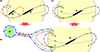 |
Fig. 13. Potential mechanism for energy transfer from solar flare to filament. In panel (a), the pre-eruptive state on 14 March after the jet1 is shown. The solid black line represents the field lines for the RF segment, whereas the orange line represents the field of the DF segment. Both segments are represented by black ellipsoids. The dashed line is the PIL. In panel (b), the DF eruption (green circle) and its magnetic structure (blue lines) are represented. The orange band is the reconnection zone under the erupted filament according to the CSHKP model. The green and blue lines represent the same field line in different phases. Both connect the points E and F. The green one is newly reconnected in the current layer of the orange band; it contracts and forms the red line. In this contraction, it reconnects with the line of the filament channel AB. The region where they reconnect is marked by a green star. In the post-reconnection evolution (c), the change in magnetic field line connectivity is observed. The filament’s original foot point A shifts to E, forming a new foot point, EB, and a post-flare loop, AF. Hot plasma transferred from the flare is represented by the greenish region east of the EB line, while the orange area on the filament indicates the subsequent brightening. |
In this paper, we aim to shed light on the mechanisms behind the triggering of large-amplitude oscillations. We find that the very energetic event of 15 March is associated with a nearby flare. The mechanism is related neither to Moreton waves nor to jets as usually reported in the literature. Actually, the energy of the flare is somehow transferred to the filament channel. This increases the pressure on one side of the filament channel, pushing the heavy prominence plasma and initiating the oscillation. Further cases need to be reported to provide insight into these mechanisms. Realistic numerical experiments are also required to understand the scenarios that produce these events. These investigations are left for future work.
Data availability
Movies associated to Figs. 1, 3, 4 and 10 are available at https://www.aanda.org
Acknowledgments
This publication is part of the R+D+i project PID2020-112791GB-I00, financed by MCIN/AEI/10.13039/501100011033. M. Luna acknowledges support through the Ramón y Cajal fellowship RYC2018-026129-I from the Spanish Ministry of Science and Innovation, the Spanish National Research Agency (Agencia Estatal de Investigación), the European Social Fund through Operational Program FSE 2014 of Employment, Education and Training and the Universitat de les Illes Balears. This research has been supported by the European Research Council through the Synergy grant No. 810218 (“The Whole Sun”, ERC-2018-SyG) and also by the Research Council of Norway through its Centres of Excellence scheme, project number 262622. CHIANTI is a collaborative project involving George Mason University, the University of Michigan (USA), University of Cambridge (UK) and NASA Goddard Space Flight Center (USA). We acknowledge NASA’s Astrophysics Data System Bibliographic Services.
References
- Adrover-González, A., Terradas, J., Oliver, R., & Carbonell, M. 2021, A&A, 649, A142 [NASA ADS] [CrossRef] [EDP Sciences] [Google Scholar]
- Arregui, I., Oliver, R., & Ballester, J. L. 2018, Liv. Rev. Sol. Phys., 15, 3 [Google Scholar]
- Asai, A., Ishii, T. T., Isobe, H., et al. 2012, ApJ, 745, L18 [NASA ADS] [CrossRef] [Google Scholar]
- Athiray, P. S., & Winebarger, A. R. 2024, ApJ, 961, 181 [NASA ADS] [CrossRef] [Google Scholar]
- Auchère, F., Soubrié, E., Pelouze, G., & Buchlin, É. 2023, A&A, 670, A66 [NASA ADS] [CrossRef] [EDP Sciences] [Google Scholar]
- Bamba, Y., Inoue, S., & Hayashi, K. 2019, ApJ, 874, 73 [NASA ADS] [CrossRef] [Google Scholar]
- Becker, U. 1958, Z. Astrophys., 44, 243 [NASA ADS] [Google Scholar]
- Benz, A. O. 2008, Liv. Rev. Sol. Phys., 5, 1 [Google Scholar]
- Bocchialini, K., Baudin, F., Koutchmy, S., Pouget, G., & Solomon, J. 2011, A&A, 533, A96 [NASA ADS] [CrossRef] [EDP Sciences] [Google Scholar]
- Bruzek, A., & Becker, U. 1957, Z. Astrophys., 42, 76 [NASA ADS] [Google Scholar]
- Carmichael, H. 1964, in The Physics of Solar Flares, ed. W. H. Hess, 451 [Google Scholar]
- Chandra, R., Filippov, B., Joshi, R., & Schmieder, B. 2017, Sol. Phys., 292, 81 [NASA ADS] [CrossRef] [Google Scholar]
- Chen, H. D., Jiang, Y. C., & Ma, S. L. 2008, A&A, 478, 907 [NASA ADS] [CrossRef] [EDP Sciences] [Google Scholar]
- Devi, P., Chandra, R., Joshi, R., et al. 2022, Adv. Space Res., 70, 1592 [NASA ADS] [CrossRef] [Google Scholar]
- Dodson, H. W. 1949, ApJ, 110, 382 [NASA ADS] [CrossRef] [Google Scholar]
- Druett, M. K., Ruan, W., & Keppens, R. 2023, Sol. Phys., 298, 134 [NASA ADS] [CrossRef] [Google Scholar]
- Druett, M., Ruan, W., & Keppens, R. 2024, A&A, 684, A171 [NASA ADS] [CrossRef] [EDP Sciences] [Google Scholar]
- Eto, S., Isobe, H., Narukage, N., et al. 2002, PASJ, 54, 481 [NASA ADS] [CrossRef] [Google Scholar]
- Foullon, C., Verwichte, E., & Nakariakov, V. M. 2009, ApJ, 700, 1658 [NASA ADS] [CrossRef] [Google Scholar]
- Freeland, S. L., & Handy, B. N. 1998, Sol. Phys., 182, 497 [Google Scholar]
- Gibson, S. E., Kucera, T. A., Rastawicki, D., et al. 2010, ApJ, 724, 1133 [NASA ADS] [CrossRef] [Google Scholar]
- Gilbert, H. R., Daou, A. G., Young, D., Tripathi, D., & Alexander, D. 2008, ApJ, 685, 629 [NASA ADS] [CrossRef] [Google Scholar]
- Hannah, I. G., & Kontar, E. P. 2012, A&A, 539, A146 [NASA ADS] [CrossRef] [EDP Sciences] [Google Scholar]
- Hershaw, J., Foullon, C., Nakariakov, V. M., & Verwichte, E. 2011, A&A, 531, A53 [NASA ADS] [CrossRef] [EDP Sciences] [Google Scholar]
- Hirayama, T. 1974, Sol. Phys., 34, 323 [Google Scholar]
- Hudson, H. S., Acton, L. W., Harvey, K. L., & McKenzie, D. E. 1999, ApJ, 513, L83 [Google Scholar]
- Hyder, C. L. 1966, Z. Astrophys., 63, 78 [NASA ADS] [Google Scholar]
- Isobe, H., & Tripathi, D. 2006, A&A, 449, L17 [NASA ADS] [CrossRef] [EDP Sciences] [Google Scholar]
- Isobe, H., Tripathi, D., & Archontis, V. 2007, ApJ, 657, L53 [NASA ADS] [CrossRef] [Google Scholar]
- Jing, J., Lee, J., Spirock, T. J., et al. 2003, ApJ, 584, L103 [NASA ADS] [CrossRef] [Google Scholar]
- Jing, J., Lee, J., Spirock, T. J., & Wang, H. 2006, Sol. Phys., 236, 97 [NASA ADS] [CrossRef] [Google Scholar]
- Joshi, R., Luna, M., Schmieder, B., Moreno-Insertis, F., & Chandra, R. 2023, A&A, 672, A15 [Google Scholar]
- Kopp, R. A., & Pneuman, G. W. 1976, Sol. Phys., 50, 85 [Google Scholar]
- Labrosse, N., Heinzel, P., Vial, J. C., et al. 2010, Space Sci. Rev., 151, 243 [Google Scholar]
- Lemen, J. R., Title, A. M., Akin, D. J., et al. 2012, Sol. Phys., 275, 17 [Google Scholar]
- Li, T., & Zhang, J. 2012, ApJ, 760, L10 [NASA ADS] [CrossRef] [Google Scholar]
- Liakh, V., Luna, M., & Khomenko, E. 2020, A&A, 637, A75 [NASA ADS] [CrossRef] [EDP Sciences] [Google Scholar]
- Liakh, V., Luna, M., & Khomenko, E. 2021, A&A, 654, A145 [NASA ADS] [CrossRef] [EDP Sciences] [Google Scholar]
- Liakh, V., Luna, M., & Khomenko, E. 2023, A&A, 673, A154 [NASA ADS] [CrossRef] [EDP Sciences] [Google Scholar]
- Liu, W., Ofman, L., Nitta, N. V., et al. 2012, ApJ, 753, 52 [NASA ADS] [CrossRef] [Google Scholar]
- Liu, Y. D., Hu, H., Wang, R., et al. 2015, ApJ, 809, L34 [NASA ADS] [CrossRef] [Google Scholar]
- Luna, M., & Karpen, J. 2012, ApJ, 750, L1 [NASA ADS] [CrossRef] [Google Scholar]
- Luna, M., & Moreno-Insertis, F. 2021, ApJ, 912, 75 [NASA ADS] [CrossRef] [Google Scholar]
- Luna, M., Díaz, A. J., & Karpen, J. 2012, ApJ, 757, 98 [Google Scholar]
- Luna, M., Knizhnik, K., Muglach, K., et al. 2014, ApJ, 785, 79 [NASA ADS] [CrossRef] [Google Scholar]
- Luna, M., Terradas, J., Khomenko, E., Collados, M., & Vicente, A. d. 2016, ApJ, 817, 157 [NASA ADS] [CrossRef] [Google Scholar]
- Luna, M., Su, Y., Schmieder, B., Chandra, R., & Kucera, T. A. 2017, ApJ, 850, 143 [NASA ADS] [CrossRef] [Google Scholar]
- Luna, M., Karpen, J., Ballester, J. L., et al. 2018, ApJS, 236, 35 [NASA ADS] [CrossRef] [Google Scholar]
- Luna, M., Mestre, J. R. M., & Auchère, F. 2022a, A&A, 666, A195 [NASA ADS] [CrossRef] [EDP Sciences] [Google Scholar]
- Luna, M., Terradas, J., Karpen, J., & Ballester, J. L. 2022b, A&A, 660, A54 [NASA ADS] [CrossRef] [EDP Sciences] [Google Scholar]
- Mazumder, R., Pant, V., Luna, M., & Banerjee, D. 2020, A&A, 633, A12 [NASA ADS] [CrossRef] [EDP Sciences] [Google Scholar]
- Moreton, G. E., & Ramsey, H. E. 1960, PASP, 72, 357 [NASA ADS] [CrossRef] [Google Scholar]
- Morgan, H., & Druckmüller, M. 2014, Sol. Phys., 289, 2945 [Google Scholar]
- Okamoto, T. J., Nakai, H., Keiyama, A., et al. 2004, ApJ, 608, 1124 [NASA ADS] [CrossRef] [Google Scholar]
- Pant, V., Mazumder, R., Yuan, D., et al. 2016, Sol. Phys., 291, 3303 [NASA ADS] [CrossRef] [Google Scholar]
- Paraschiv, A. R., Donea, A. C., & Judge, P. G. 2022, ApJ, 935, 172 [NASA ADS] [CrossRef] [Google Scholar]
- Pesnell, W. D., Thompson, B. J., & Chamberlin, P. C. 2012, Sol. Phys., 275, 3 [Google Scholar]
- Pouget, G. 2007, Ph.D Thesis, Paris, France [Google Scholar]
- Raes, J. O., Van Doorsselaere, T., Baes, M., & Wright, A. N. 2017, A&A, 602, A75 [NASA ADS] [CrossRef] [EDP Sciences] [Google Scholar]
- Saqri, J., Veronig, A. M., Heinemann, S. G., et al. 2020, Sol. Phys., 295, 6 [Google Scholar]
- Schmieder, B., Malherbe, J. M., & Raadu, M. A. 1985, A&A, 142, 249 [NASA ADS] [Google Scholar]
- Schou, J., Scherrer, P. H., Bush, R. I., et al. 2012, Sol. Phys., 275, 229 [Google Scholar]
- Schutgens, N. A. J., & Toth, G. 1999, A&A, 345, 1038 [NASA ADS] [Google Scholar]
- Shen, Y., Ichimoto, K., Ishii, T. T., et al. 2014a, ApJ, 786, 151 [NASA ADS] [CrossRef] [Google Scholar]
- Shen, Y., Liu, Y. D., Chen, P. F., & Ichimoto, K. 2014b, ApJ, 795, 130 [Google Scholar]
- Shibata, K., & Magara, T. 2011, Liv. Rev. Sol. Phys., 8, 6 [Google Scholar]
- Sindhuja, G., Singh, J., Asvestari, E., & Raghavendra Prasad, B. 2022, ApJ, 925, 25 [NASA ADS] [CrossRef] [Google Scholar]
- Sturrock, P. A. 1966, Nature, 211, 695 [Google Scholar]
- Takahashi, T., Asai, A., & Shibata, K. 2015, ApJ, 801, 37 [NASA ADS] [CrossRef] [Google Scholar]
- Vršnak, B., Veronig, A. M., Thalmann, J. K., & Žic, T. 2007, A&A, 471, 295 [NASA ADS] [CrossRef] [EDP Sciences] [Google Scholar]
- Wang, R., Liu, Y. D., Zimovets, I., et al. 2016a, ApJ, 827, L12 [NASA ADS] [CrossRef] [Google Scholar]
- Wang, Y., Zhang, Q., Liu, J., et al. 2016b, J. Geophys. Res. (Space Phys.), 121, 7423 [NASA ADS] [CrossRef] [Google Scholar]
- Xue, Z. K., Yan, X. L., Qu, Z. Q., & Zhao, L. 2014, ASP Conf. Ser., 489, 53 [NASA ADS] [Google Scholar]
- Zhang, Q. M., Chen, P. F., Guo, Y., Fang, C., & Ding, M. D. 2012, ApJ, 746, 19 [NASA ADS] [CrossRef] [Google Scholar]
- Zhang, Q. M., Chen, P. F., Xia, C., Keppens, R., & Ji, H. S. 2013, A&A, 554, A124 [NASA ADS] [CrossRef] [EDP Sciences] [Google Scholar]
- Zhang, Q. M., Li, D., & Ning, Z. J. 2017, ApJ, 851, 47 [NASA ADS] [CrossRef] [Google Scholar]
- Zhang, L. Y., Fang, C., & Chen, P. F. 2019, ApJ, 884, 74 [Google Scholar]
- Zhou, Y.-H., Xia, C., Keppens, R., Fang, C., & Chen, P. F. 2018, ApJ, 856, 179 [Google Scholar]
- Zurbriggen, E., Cécere, M., Sieyra, M. V., et al. 2021, Sol. Phys., 296, 173 [NASA ADS] [CrossRef] [Google Scholar]
Appendix A: Considerations on thread dynamics and energetics
We use a modified version of the model described in Adrover-González et al. (2021) to show the basic physics behind the energization of the thread and the subsequent relaxation phase that involves the large amplitude thread oscillations.
We consider the prominences to be composed of magnetic flux tubes with dense cold plasma threads in them. On both sides of the cold thread, the tube has a coronal temperature and is often referred to as the evacuated regions. The flux tubes have dips in their central part and an equilibrium situation the threads will reside at the bottom of these dips. The movement of the threads is along the tube and can be modelled as a 1D system. The main equation of our system is the momentum equation
with s being the coordinate of the centre of the thread along the fluxtube, ρt the thread density and g∥ the gravity projection along the magnetic field line.
We approximate the gas pressure derivative by
where we have assumed that the thread does not change its shape and keeps its length, lt, constant. Let us suppose that on the left part of the tube, denoted by the subindex 1, and due to the energisation process gas pressure is increasing and reaches a maximum value pmax, i.e. p1 = pmax. This pressure excess pushes the thread to the right and produces a compression on the evacuated part, denoted by the subindex 2. We assume that the compression of this part of the tube, which initially had a pressure p0, is adiabatic, therefore we have that
Note that if s = L/2 the thread is its initial equilibrium position, and p2 = p0. We aim at finding the new position equilibrium due to the supplied pressure excess. Writing s = L/2 + δse the previous expression is approximated by
valid for the situation δse ≪ L − lt. Using this linear approximation we have that
where we have used the definition of the coronal sound speed, cs02 = γp0/ρ0.
For the gravitational term in Eq. (A.1) we consider the approximated expression from Luna et al. (2022b) where it is assumed that the dips have a circular geometry of radius R
and R⊙ is the solar radius. From the equilibrium condition we have
and using the previously derived linear approximations we obtain the following thread displacement
When moving along the dip field line, the thread increases its height with respect to the bottom of the dip which is approximately

Here it should be noted that (A.7) condition gives a lower value for the δse (A.8) displacement. This is because the thread would overshoot the point where the forces cancel out. The condition to find δse would be the point where the velocity becomes zero. However, it is not possible to find an analytical solution and we consider Eq. (A.8) a reasonable approximation or a lower value. Just at the position of maximum displacement is when the system has the maximum energy. The pressure exerted by the flare is still pmax and the total energy of the system is the sum of the internal energies of the evacuated parts of the tube plus the potential energy of the thread at height h (since the internal energy of the dense thread does not change it is not taken into account in the computation), namely,
Each term contains the length of the segment that represents and we have taken into account that the right leg has gone through an adiabatic compression.
In the second phase of the process proposed in the present paper as the trigger of the oscillations we assume that the overpressure that has displaced the thread a distance δse, suddenly disappears and the thread tends to return to its initial position at L/2. We are interested in the calculation of the maximum velocity while it is oscillating around L/2 since this is a parameter that can be compared with the observational data. Energy conservation allows us the determine the maximum velocity. In this phase, the pressure drops because we assume that the flare stops injecting hot plasma into the left side of the tube. We assume that the pressure transitions from pmax to an ambient atmospheric value p0. Just after the sudden pressure decrease to p0, the total energy of the system is, similarly to Eq. (A.10),

This expression is now written in terms of δse using the same approximations as before and reducing to
As the thread returns to its equilibrium position s = L/2 located at the bottom of the dip, it acquires kinetic energy associated with its velocity v. The left part of the tube is compressed adiabatically. In this case, the total energy is
This expression must be equal to Eq. (A.12) because of energy conservation (ET = ET′); this allows us to obtain the simple expression (valid when δse ≪ L − lt)
where Δh is given by Eq. (A.9).
An estimation of the energy of a solar flare can be calculated using the total energy (A.10) and subtracting the energy at equilibrium (s = L/2):
This equation represents the energy contributed by the flare per unit area to each magnetic flux tube. The total number of tubes or filaments is estimated by assuming a typical prominence mass (Mprom) and dividing it by the mass of an individual filament (ρthlth). With this, we can assess a lower bound of the flare energy as
Appendix B: Pendulum model for longitudinal solar prominence oscillations
In this appendix, we briefly describe the pendulum model by Luna et al. (2022b). The longitudinal oscillations in prominences are characterised by the 1D displacements of the constituent threads along the magnetic flux tubes. We assume a low-β, adiabatic plasma confined within flux tubes of uniform cross-section, aligned along a static magnetic field, with no heating or radiative terms included. Luna et al. (2012) demonstrated that, in contrast to the usual MHD slow modes, both the gas-pressure gradient and gravity are the restoring forces for these modes. From the ideal MHD equations
where  is the sound speed and p and ρ are the equilibrium gas pressure and density, respectively. The gravity projected along the magnetic flux tube is g∥(s). Assuming a harmonic time dependence, eiωt, the governing equation becomes
The novelty introduced by Luna et al. (2022a) is that the intrinsic spatial variations of the solar gravity field are considered g = g(r) in contrast with the usual assumption of uniform gravity in Cartesian geometry. Additionally, it is assumed that prominences are located at the lower corona where r ≈ R⊙, with r being the radial distance to the solar centre and R⊙ the solar radius. Thus,  , where
  is the radial unit vector pointing in the (minus) direction of gravity and g0 = 274 km s−1s the gravitational acceleration at the solar surface. This assumes that, for filaments in the low corona, the main spatial variation of gravity is due to its changing direction, not its intensity because the radial distance r is not changing considerably. Assuming that dips have a semicircular geometry with radius of curvature R and under some approximations (see Sect. 3.1 from Luna et al. 2022a) the projected gravity is
Note that on the right-hand side, the first term is associated with the change of magnetic-field direction along the line and the second is associated with the intrinsic variation of nonuniform gravity. Substituting Eq. (B.3) into Eq. (B.2) we obtain a dispersion relation that can be approximated as
where ωslow is the slow-mode angular frequency associated with the gas-pressure gradient. Luna et al. (2012) showed that the last term associated with slow modes is relatively small and can be neglected. Additional works supported this finding (see Zhang et al. 2013; Luna et al. 2016; Zhou et al. 2018; Zhang et al. 2019; Liakh et al. 2021). Neglecting the slow mode contribution, Eq. (B.4) can written in terms of the period (ω = 2π/P) as
where
This corresponds to the oscillation period of a thread in a straight horizontal tube. In contrast to the uniform gravity case, gravity still has a non-zero projection along the tube. From Eq. (B.5) we find

which is a useful equation for determining the radius of curvature of the dip when the oscillation period is known.
This model also predicts a minimum value for the magnetic field strength of the prominence, assuming that the magnetic field tension supports the cool, dense prominence threads. Consequently, the magnetic tension must be greater than the weight of the threads, such that
Eq. (B.7) yields the following relation:
Using this expression, the magnetic field strength at the dip of the field lines supporting the prominence can be estimated.
All Tables
Best-fit and seismology parameters of the three oscillations reported in this work.
All Figures
|
Fig. 1. Temporal evolution on 14 March 2015 in SDO-AIA 171 Å (left column), 193 Å (central column), and in GONG Hα (right column). In panel (b), the images are overlaid with the HMI magnetogram of the AR. In the same panel, an inset shows a detail of the HMI magnetogram around the AR central bipole. It consists of a bipole with a positive polarity (P, in red) surrounded by negative polarities (N, in dark blue). In panel (c), the image is shown in Hα with a large F filament studied in this work and a small f filament in the AR. The f eruption is related to the first jet on this day. In panels (d) and (e), jet1 appears as a bright structure, marked with the white arrow. It is visible in the AIA pass bands, but not in the Hα; see panel (f). After the impact of the jet1, the F filament splits into two segments. In the AIA channels ((g) and (h)), both parts can be seen, but it is much clearer in Hα (i). The segments are labelled RF and DF. The DF segment detaches from the body of the initial filament and is ejected up and towards the south. This segment will erupt the next day. In panel (h), inset, a detail of DF is shown. This reveals the structure of the filament in the form of threads oriented along the NW direction. An animation of this figure is available online. |
| In the text | |
|
Fig. 2. Succession of flares from AR 12297 on March 14–15 2015 registered by GOES. The GOES classification of flares measures the peak flux in the 1–8 Å range (black curve) and in the 0.5–4 Å range (red curve). The vertical blue arrows show the recurring solar flares from AR 12297 for the period from March 14 10:00 UT until March 15 6:00 UT. The two green boxes delimit the two flare events we are interested in. The first event contains one C2.6 flare, whereas the second includes two flares, of class C2.4 and C9.2, respectively. Jet1 occurs almost simultaneously after the C2.6 flare on day 14, whereas jet2 erupts just after flare C2.4 on day 15. |
| In the text | |
|
Fig. 3. Temporal evolution on 15 March 2015; similar to Fig. 1. Panels (a) and (b) show the jet2 marked by a white arrow. In both AIA panels, the plasma is seen by absorption. A dark structure is also seen in panel (c). In panel (c), the two filament segments are seen. Jet2 hits DF and triggers its eruption. In the middle row, DF (white arrow) is slowly rising. In the last column, the fulguration associated with the DF eruption is occurring. In (g) and (h), the postflare loops are visible. In panel (i), chromospheric brightenings are also seen. These brightenings form two ribbons, one north and one south, although the shape is not well defined. It is clearer in later times and we recommended consulting the animation accompanying this figure. In panel (i), the RF segment has an elongated shape because it is pushed in a NW direction. An animation of this figure is available online. |
| In the text | |
|
Fig. 4. Temporal evolution of DF eruption and the triggering of the oscillations in the RF segment in 171 Å data. In panel (a), the absorbing plasma of the RF and DF segments shown in the figure is visible. In the same panel, the white box delimits the area where jet2 is located. In panel (b), DF jet2 has already impacted DF, and this segment is already erupting. Jet2 also impacts RF, producing a slight brightening in a small area on the RF spine (blue arrow). During the eruption of DF, it seems that changes also occur in RF, such as the appearance of a protrusion on its west side (green arrow). This same protrusion (green arrow) becomes bright shortly afterwards. In panel (d), within the white box, a lot of brightening can be seen on RF. In the next panels, from (e) to (h), the brightenings are massive over the whole structure, and in (i) loops can be seen in the NW area (green arrow) outlining a kind of flux rope structure. An animation of this figure is available online. |
| In the text | |
|
Fig. 5. AIA 171 Å image showing the artificial slits S1 and S2 used to study the oscillations on DF and RF, respectively. S1 has a width of 4 arcsecs, whereas S2 has a width of 10 arcsecs. The figure shows jet1 (white arrow) interacting with the filament. This jet will split the filament in two: DF and RF (see Fig. 1). However, this shows an early stage, and DF has not yet moved to its new position under the S1 slit. Part of the jet1 flows are directed in a NW direction along S2. The inset shows the white box area enlarged to show the details of the NW-bound jet. |
| In the text | |
|
Fig. 6. Time-distance diagrams of March 14 constructed with the artificial slits shown in Fig. 5. In panel (a), the diagram for S1 over DF is shown, and in panel (b), the diagram in S2 over RF is shown both panels in AIA 171Å. In this pass band, the prominence plasma appears in absorption as dark bands. The white dashed line shows the oscillation fit using Eq. (1). The best-fit parameters of the oscillation are shown over both panels. In panel (b), the fit is also shown by plotting jet1 with a red dashed line. This gives the jet propagation velocity shown in the panel. |
| In the text | |
|
Fig. 7. AIA 171 Å image showing filament on 15 March, similarly to Fig. 5. The artificial slits S3 and S4 are shown. S3 is used to study the propagation of jet2, while S4 is used to study the oscillations of the RF segment. Both slits have a width of 10 arcsecs. |
| In the text | |
|
Fig. 8. Similar to Fig. 6, but with the time-distance diagram in 171 Å along slit S4 shown. The oscillation best-fit parameters are shown in the figure with the white dashed line. Bright structures are seen between 01:10 and 02:10 UT, which is the impulsive phase when the oscillation is triggered. After 2:10 UT, the absorbing plasma in the filament moves periodically around y = 120 arcsecs. Between 6:30 and 7:20 UT, there is a gap with no SDO data. |
| In the text | |
|
Fig. 9. Time-distance diagram for jet2 along the artificial slit S3 (Fig. 7) in 171 Å (panel a), 131 Å (panel b), and 94 Å (panel c). In all the panels, the two vertical grey lines mark the times of the first C2.4 flare at 00:34UT and the second C9.2 flare starting at 01:15UT. Also in the three panels, by fitting a straight line (red dashed line) we estimate the speed of the jet2 flows on each pass band. The jet2 propagation velocities are shown in each panel. The average value for all three pass bands is 235 km s−1. |
| In the text | |
|
Fig. 10. Plot showing two moments during triggering of huge oscillation in AIA 171 Å, 131 Å, and 94 Å. The images have been processed using the WOW technique described in Sect. 2. The left column shows the region at 1:33 UT. In 171 Å (a) the structures already discussed in Fig. 4 are visible. In 131 Å (c), however, the post-flare loops around the flare are visible, as well as bright tubes in this pass band from the flare area to the filament. The white arrows indicate the region where the bright tubes appear in 131 Å and 94Å. These appear to trace a twisted field line reminiscent of a magnetic rope. Similar structures can be seen in 94 Å (e). Later, in the right column, the structure has evolved, but the bright tubes connecting to the prominence at both wavelengths are still clear. We note that these bright tubes are not visible in 171 Å. In 171 Å, the white arrows show the areas where the tubes appear in 131 Å and 94 Å. An animation of this figure is available online. |
| In the text | |
|
Fig. 11. Temperature analysis of small region shown in the box in panel (a). In panel (b), the temperature analysis of that area using DEM is shown. In panel (c), the average intensity in the same area of all AIA wavebands is shown. The colours used are inspired by the respective AIA channel palette. |
| In the text | |
|
Fig. 12. Details of brightening observed in prominence in AIA 171 Å, 131 Å, and 94 Å pass bands. The region corresponds to the white box in Fig. 4d. The green arrows show the bright fibril-like structures at the southern edge of the prominence. |
| In the text | |
|
Fig. 13. Potential mechanism for energy transfer from solar flare to filament. In panel (a), the pre-eruptive state on 14 March after the jet1 is shown. The solid black line represents the field lines for the RF segment, whereas the orange line represents the field of the DF segment. Both segments are represented by black ellipsoids. The dashed line is the PIL. In panel (b), the DF eruption (green circle) and its magnetic structure (blue lines) are represented. The orange band is the reconnection zone under the erupted filament according to the CSHKP model. The green and blue lines represent the same field line in different phases. Both connect the points E and F. The green one is newly reconnected in the current layer of the orange band; it contracts and forms the red line. In this contraction, it reconnects with the line of the filament channel AB. The region where they reconnect is marked by a green star. In the post-reconnection evolution (c), the change in magnetic field line connectivity is observed. The filament’s original foot point A shifts to E, forming a new foot point, EB, and a post-flare loop, AF. Hot plasma transferred from the flare is represented by the greenish region east of the EB line, while the orange area on the filament indicates the subsequent brightening. |
| In the text | |
Current usage metrics show cumulative count of Article Views (full-text article views including HTML views, PDF and ePub downloads, according to the available data) and Abstracts Views on Vision4Press platform.
Data correspond to usage on the plateform after 2015. The current usage metrics is available 48-96 hours after online publication and is updated daily on week days.
Initial download of the metrics may take a while.