© The Authors 2024

1 Introduction

Simple molecular ions, such as HCO⁺ and N₂H⁺, found in dense interstellar clouds are manifestations of gas-phase chemistry driven by cosmic-ray ionisation. The ionisation of H₂, the principal constituent of these clouds, leads immediately to the formation of the trihydrogen cation, ${\text{H}}_3^{+}$. This triangular cation is observable by its rovibronic spectrum in diffuse clouds in absorption against strong infrared background sources but is difficult to detect in highly obscured, dense regions. On the other hand, ${\text{H}}_3^{+}$ is easily destroyed in exothermic proton transfer reactions with the common neutral species CO, N₂, and HD; these reactions produce HCO⁺, N₂H⁺, and H₂D⁺, which are observable in cold, dark clouds owing to their pure rotational spectra. Reactions of CO and N₂ with H₂D⁺, or the doubly and triply deuterated forms D₂H⁺ and ${\text{D}}_3^{+}$, then produce DCO⁺ and N₂D⁺. Because of the relatively simple chemical network connecting these molecules to the primary ions, HCO⁺ and N₂H⁺, and more recently also H₂D⁺, have been used to estimate the electron abundance, X(e⁻), and the cosmic-ray ionisation rate of H₂, ${\zeta }_{{\text{H}}_2}$, in dense interstellar clouds. The methods generally involve estimates of the abundances of CO, N₂, and other major destroyers of ${\text{H}}_3^{+}$, and often combine them with the fractionation ratios DCO⁺/HCO⁺ or N₂D⁺/N₂H⁺ to derive the electron fraction and the ${\text{H}}_3^{+}$ abundance in the cloud (e.g. Guelin et al. 1977; Wootten et al. 1979; Caselli et al. 1998, 2002, 2008; van der Tak & van Dishoeck 2000; Bovino et al. 2020; Redaelli et al. 2021; Sabatini et al. 2023). The usefulness of analytic formulas for deriving ${\zeta }_{{\text{H}}_2}$ from the observed fractionation ratios is discussed in Redaelli et al. (2024). Ionising collisions with energetic particles have a fundamental influence on the physics and chemistry of interstellar molecular clouds (Padovani et al. 2020). The ionisation of H₂ is dominatedby low-energy particles (<1 GeV/nucleon), mainly protons and their secondary electrons. Cosmic ray propagation models predict that the total ionisation rate of H₂ decreases with an increasing H2 column density of the medium, from values estimated in diffuse clouds, ~10⁻¹⁶−10⁻¹⁵ s⁻¹ (Indriolo & McCall 2012; Neufeld & Wolfire 2017), down to ~10⁻¹⁷ s⁻¹ at the column densities characteristic of dense cores, N(H₂) ~ 10²³ cm⁻² (Padovani et al. 2009, 2018, 2024; Ivlev et al. 2015, 2021).

Besides its central role in astrochemistry, cosmic-ray ionisation is also the dominant direct heating mechanism of gas in quiescent regions shielded from UV radiation. The gas temperature in these regions is determined by the equilibrium between the cosmic-ray ionisation rate, the rate of gas cooling by line emission, and the transfer rate of energy due to collisions between gas particles and dust grains (Burke & Hollenbach 1983; Goldsmith 2001; Galli et al. 2002). Conversely, gas temperature measurements can also be used to constrain the cosmic-ray ionisation rate (Galli & Padovani 2015; Ivlev et al. 2019).

In addition to their potential use for estimating the cosmic-ray ionisation rate, the deuterated isotopologues of ${\text{H}}_3^{+}$ are predicted to be useful probes of the interiors of molecular cloud cores (Caselli et al. 2003; Roberts et al. 2003; Walmsley et al. 2004; Vastel et al. 2006b). The detection of H₂D⁺ and D₂H⁺ in centrally condensed starless cores (Caselli et al. 2003; Vastel et al. 2004, 2006a; Parise et al. 2011) shows that these light deuterated ions with permanent electric dipole moments can retain high abundances in very dense, cold gas, where many C-, N-, and O-bearing molecules are frozen onto dust grains.

Here we present maps of the pre-stellar core Ophiuchus/H-MM1 in the λ = 0.8 mm lines of ortho-H₂D⁺ (hereafter oH₂D⁺), N₂H⁺, and DCO⁺, obtained using the Large APEX sub-Millimeter Array (LAsMA) of the Atacama Pathfinder EXperiment (APEX) telescope. The ground-state lines of oH₂D⁺ and para-D₂H⁺ (hereafter pD₂H⁺) have previously been detected towards this core (Parise et al. 2011), and a Very Large Array (VLA) mapping shows severe depletion of ammonia in its centre (Pineda et al. 2022). The goal of the present observations is to derive the distributions of the oH₂D⁺, N₂H⁺, and DCO⁺ in the core, test the predictions of chemistry models concerning their abundances, and put constraints on the cosmic-ray ionisation rate in the region.

2 Observations

The H-MM1 core was mapped with the LAsMA array on APEX using a frequency set-up that covered the rotational lines oH₂D⁺(1₁₀ − 1₁₁), N₂H⁺(4 − 3), and DCO⁺(5 − 4) at λ = 0.8 mm. This was achieved by tuning the upper sideband of the dual-sideband receiver to 372.6 GHz. The frequencies, upper-state energies, and the critical densities of the observed transitions are listed in Table 1. The backend was composed of fast Fourier transform spectrometers (FFTS4G) that covered two 4 GHz intermediate frequency bands resolved into 65 536 spectral channels of 61.03 kHz in width, corresponding to ~49 m s⁻¹ at 372.4 GHz. The observations were done between June 3 and July 2, 2023, under the project number M-0111.F-9508A-2023. The APEX telescope is located at an altitude of 5100 m at Llano de Chajnantor, in Chile.

The LAsMA array has 7 pixels separated by approximately 40″. The mapping was performed in the on-the-fly (OTF) mode. The scanning direction was alternated between equatorial east-west and north-south. The separation between rows and columns was 5″.6, equalling to one third of the beam width at 372.4 GHz. With a scanning speed of 5″.6 s⁻¹ and a dump time of 1 s, the dump step was equal to the separations between rows and columns. The coordinates of the map centre are RA 16^h27^m59″.6, Dec −24º33′40″ (J2000.0). This position lies ~15″ east of the density peak of the core, RA 16^h27^m58″.65, Dec -24º33′41.2″, which is used as (0,0) of the maps presented in this paper.

The distribution of the sampled positions is pseudo-random, and to form image cubes, the observations were interpolated and averaged to a regular grid with a cell size of 5″.6. Following the recommendation of Mangum et al. (2007), we used as the grid-ding function a Bessel function of the first kind, J₁, tapered with a Gaussian. In practice, the observation representing a certain grid position was obtained by accumulating all observations with a radius of three cell widths (one full width at half maximum of the telescope beam) from this position, weighted by the function J₁(πr/a)/(πr/a) × exp(−(r/b)²), where r is the distance from the grid position in units of the cell size, and the constants are a = 1. 55, b = 2.52. Even though the operation corresponds to a convolution with this function, it causes a minimal broadening of the effective beam (when the grid spacing is sufficiently small), and thus preserves the observed intensity (see Fig. 6 of Sawada et al. 2008). In addition to the gridding function, the accumulated spectra were weighted by the inverse square of the system noise temperature, T_SYS (the integration time was 1 s for all spectra). The size of the gridded area is approximately 120″ × 150″. This region is shown in Fig. 1 as a rectangle superposed on the H₂ column density and dust colour temperature maps derived using high-resolution (HiRes) sub-millimetre images from the Spectral and Photometric Imaging Receiver (SPIRE) instrument of the Herschel Space Observatory (Griffin et al. 2010). The HiRes images are produced by applying a beam-deconvolution method to standard pipeline processed calibrated Herschel-SPIRE maps, and they typically have a factor of two higher resolution than the original maps¹.

3 Spectra and maps

The oH₂D⁺(1₁₀ − N₂H⁺(4 − 3), and DCO⁺(5 − 4) spectra towards the core centre are shown in Fig. 2. Each spectrum represents one cell of the image cube constructed from the OTF observations as described in Sect. 2, and corresponds to an integration towards the grid positions with a ~ 18″ beam. The spectra are presented on the T_MB scale. Based on measurements performed in 2023, available on the APEX website², we assumed that the main-beam efficiency of the telescope, η_MB, is 0.74 at the frequencies of the oH₂D⁺ and N₂H⁺ lines, and 0.75 at the frequency of the DCO⁺ line. The hyperfine structures of the transitions are indicated with red bars. The frequencies and the relative intensities of the hyperfine components were adopted from Jusko et al. (2017) and Jensen et al. (1997) for H₂D⁺, and from Pagani et al. (2009a) for N₂H⁺. For DCO⁺; they were taken from the Jet Propulsion Laboratory of California Institute of Technology service for molecular spectroscopy.³ The spectroscopic parameters of this molecule were derived by Caselli & Dore (2005) and Lattanzi et al. (2007).

The integrated intensity maps shown in Fig. 3 reflect the spatial distributions of the molecules and the excitation conditions (the density and temperature) in the cloud. The lines are integrated over the local standard of rest (LSR) velocity range 3.3−5.1 km s⁻¹. The emission in oH₂D⁺(1₁₀ − is the brightest and most extended of the three lines observed. There we see a peanut-shaped maximum centred some 5″ south-west of the density peak (our (0,0)), and another maximum around the offset ~(+10″, +30″). The emission in N₂H⁺ (4 − 3) is relatively compact and peaks ~5″ east of (0,0). The secondary N₂H⁺ peak in the north-east coincides with the secondary oH₂D⁺ peak. The DCO⁺(5 − 4) map has three peaks, located at the offsets ~(+10″, −10″), ~(+15″, +20″), and ~(+20″, +45″). The emission is shifted approximately 10″ to the east with respect to the oH₂D⁺ emission. This shift is illustrated in Fig. 4, where the DCO⁺ contours are superposed on the oH₂D⁺ pixel map.

The line parameters derived by Gaussian fits to the hyperfine structure components are presented in Table 2. In this calculation, it was assumed that all hyperfine components have the same intrinsic linewidth, and that the populations of the hyperfine states are proportional to their statistical weights. The linewidth, ∆V, listed in Table 2 is the full width at half maximum (FWHM) of a single hyperfine component obtained from the Gaussian fit. The velocity dispersion of the light H₂D⁺ molecule (m ~ 4 amu) is probably dominated by thermal motion. The linewidth implies a maximum kinetic temperature of 11.2 ± 1.0 K. The hyperfine structure fits give reasonable, albeit uncertain, estimates for the total optical thicknesses, τ (the sum of the peak optical thicknesses of all components), and the excitation temperatures T_ex, of the transitions. Assuming line-of-sight homogeneity and that the T_ex is the same for all rotational transitions of the molecule, one obtains column densities given in the last column of Table 2. For N₂H⁺ and DCO⁺, the uncertainties propagated to the column density estimates are quite large. Using a broader, Gaussian gridding kernel (with $\sigma =\sqrt{2}\times$ the cell size) that results in a resolution of ~25″, the relative uncertainties are alleviated somewhat, and we get N(oH₂D⁺) = (1.3 ± 0.2) × 10¹³cm⁻², N(N₂H⁺) = (6.3 ± 2.2) × 10¹² cm⁻², and N(DCO⁺) = (2.0 ± 0.5) × 10¹³ cm⁻² at (0,0). Combined with the H₂ column density derived from Herschel, ~6 × 10²² cm⁻², these column densities imply the following fractional abundances: X(oH₂D⁺) ~ 2.2 × 10⁻¹⁰, X(N₂H⁺) ~ 1.0 × 10⁻¹⁰, and X(DCO⁺) ~ 3.3 × 10⁻¹⁰. Given the large formal errors, and the uncertain assumptions involved in the local thermodynamic equilibrium (LTE) method, we estimated abundances by modelling line emission maps.

The centroid LSR velocity and the velocity dispersion maps derived from hyperfine structure fits to the observed lines are presented in Fig. A.1. The fits are made to image cubes created by the GILDAS⁴ task xy_map from the reduced spectra with the /nogrid option. Here we assumed optically thin emission (by fixing the total optical thickness to 0.1) to avoid an eventual degeneracy between the τ and the linewidth. The pixel size corresponds to the grid step 5″.6. In addition to maps from the oH₂D⁺(1₁₀ − 1₁₁), N₂H⁺ (4 − 3), and DCO⁺(5 − 4) lines, we also include the corresponding distributions of the NH₃(1,1) lines observed with the VLA by Pineda et al. (2022). The resolution of the NH₃ mapping was 6″, but these data have been resampled to the grid used for the present LAsMA maps. The original V_LSR and σ_V maps from the VLA are shown in Fig. 3 of Pineda et al. (2022). The line parameters could be derived accurately only for a small portion of each LAsMA map. The VLA NH₃ maps are more extended and of better quality. Nevertheless, the LAsMA maps show the same basic features as seen on the VLA map: 1) the most red-shifted gas is found in an elongated region pointing towards the core centre in the centroid LSR velocity maps (upper panels), and 2) a region with low velocity dispersion can be discerned in the northern part of the core in the σ_V maps (lower panels).

Fig. 1 H2 column density and dust colour temperature (TC) maps of H-MM1 derived from Herschel-SPIRE HiRes data. The rectangle shows the area covered by the grid used for the line maps derived from the OTF observations. The circle shows the effective beam size (FWHM) of the SPIRE HiRes maps at 500 µm. The plus sign shows the location of the H2 column density peak of the core, used as (0,0) in the molecular line maps.

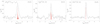Fig. 2 oH2D+ (110 − In), N2H+ (4 − 3), and DCO+ (5 − 4) spectra towards the density peak of the core. The red bars indicate the hyperfine structure components of the line.

Fig. 3 Integrated oH2D+ (110 − N2H+ (4 − 3), and DCO+ (5 − 4) line intensity maps of H-MM1. The contours are: 0.10 to 0.25 by 0.03 K km s−1 (oH2D+); 0.06 to 0.14 by 0.02 K km s−1 (N2H+ ); and 0.05 to 0.11 by 0.02 K km s−1 (DCO+). The intensity scale is $T_{\text{A}}^{*}$.

Fig. 4 Integrated oH2D+ (110 − 111) line intensity maps of H-MM1 with the DCO+ (5 − 4) contours superposed. The contour levels are the same as in Fig. 3.

4 Core model

We updated the three-dimensional model for H-MM1 described in Pineda et al. (2022). As before, the model is based on a H₂ column density map with a resolution of 6″ derived from 8 µm absorption observed by Spitzer, combined with 850 µm emission map from SCUBA and the dust colour temperature (T_C) map from Herschel (see Appendix A of Harju et al. 2020). Instead of original Herschel/SPIRE maps used previously, we calculated the T_C map from deconvolved SPIRE HiRes images, having an angular resolution of approximately 15″ (instead of ~38″ achieved previously)⁵. This resolution corresponds to the SCUBA beam at 850 µm. Moreover, as the N(H₂) map from Spitzer misses extended structures, we combined it with the extended N(H₂) map derived from SPIRE HiRes at 250, 350, and 500 µm. The SPIRE data were downloaded from the Herschel Science Archive⁶. The N(H₂) and the T_C maps of H-MM1 derived from the SPIRE HiRes data with ~15″ resolution are shown in Fig. 1. The N(H₂) map resulting from combining the Spitzer and SPIRE HiRes data is shown in Fig. 5. There, the angular resolution is 6″ in the core region, and 15″ around it.

The density distribution of the core was derived from the N(H₂) map shown in Fig. 5 by fitting Plummer-type profiles to horizontal cuts of the nearly north-south-oriented dense ridge of H-MM1. The inversion method is adopted from Arzoumanian et al. (2011), and described in some detail in Appendix D of Pineda et al. (2022). The density model was then immersed in the interstellar radiation field to compute the dust temperature distribution. The assumptions about radiation field were the same as used previously in Harju et al. (2020, see their Appendix B), that is, it consists of an isotropic component and radiation from a B star (HD 147889) located on the western side of the core approximately 1.2 pc away. The distributions of the average density and dust temperature as functions of the radial distance from the density maximum of the core are shown in Fig. 6. As in Pineda et al. (2022), we assumed that in the outer parts of the core the gas temperature is lower than the dust temperature because of molecular line cooling. Based on the T_kin distribution derived from NH₃, we assumed the gas temperature does not rise above 11 K. The assumed gas temperature profile is shown with a green curve in Fig. 6.

To predict line intensity maps from the core model requires assumptions about molecular abundances. The simplest assumption is that the fractional abundance of a molecule is constant throughout the cloud. We tested this assumption using the estimates towards our (0,0) position from the LTE method described in Sect. 3. While the predicted line intensities using these constant abundances are comparable to those observed in the core centre, the extent of the emission is clearly more compact than observed. This indicates that the fractional abundances of all three molecules are higher in the outer parts than in the centre of the core. In what follows, we use a chemical model to predict the abundance profiles of the observed molecules in the core, given the density and temperature distributions derived above.

Fig. 5 H2 column density map of H-MM1 derived by combining the 8 µm surface brightness map observed with Spitzer with SPIRE HiRes far-infrared maps. The angular resolution is 6″ in the central parts of the map, and 15″ on the outskirts. The effective beam sizes are shown in the bottom-right corner. The box shows the region covered by the molecular line maps.

5 Chemistry model

We used the gas-grain chemical model pyRate for the simulations; it is described in Sipilä et al. (2019), Riedel et al. (2023), and Harju et al. (2024). We assumed constant chemical desorption with 1% of exothermic surface reactions leading to desorption, and adopted the proton hop chemical network in the gas phase (Sipilä et al. 2019). In this model, proton donation and abstraction reactions involving O, C, and N are assumed to proceed via the exchange of one proton (or deuteron) between the reactants, without multiple atom exchanges. On the other hand, full scrambling is assumed for the ${\text{H}}_3^{+}+{\text{H}}_2$ reaction system and its deuterated variants, and the rate coefficients and branching ratios for these reactions are adopted from Hugo et al. (2009). In the chemical calculations we employed a one-dimensional physical model for H-MM1, which was constructed using the average densities and temperatures over concentric shells shown in Fig. 6. We adopted the same initial abundances as in Sipilä et al. (2019), and the simulation parameters were also the same as in that paper except for the cosmic-ray ionisation rate of H₂, ${\zeta }_{{\text{H}}_2}$, for which we tested different values ranging from 10⁻¹⁸ s⁻¹ to 10⁻¹⁵ s⁻¹. We assumed that ${\zeta }_{{\text{H}}_2}$ is constant throughout the core because the column densities in the core region (at the resolution achieved here) are confined to a narrow range, N(H₂) ~ 10²² cm⁻²−6 × 10²² cm⁻², where attenuation models (e.g. Padovani et al. 2018) do not predict drastic changes in ${\zeta }_{{\text{H}}_2}$. Besides, the angular resolution of the observations is not sufficient for studying spatial variations of ${\zeta }_{{\text{H}}_2}$. The adopted abundances of oxygen, carbon, and nitrogen relative to hydrogen are O/H = 1.8 × 10⁻⁴, C/H = 7.3 × 10⁻⁵, and N/H = 5.3 × 10¯⁵. Previous observations of ammonia and its deuter-ated forms towards H-MM1 have been reproduced well by these abundances (Harju et al. 2017, 2024; Pineda et al. 2022). We also tested higher elemental abundances (O/H = 2.56 × 10⁻⁴, C/H = 1.2 × 10⁻⁴, and N/H = 7.6 × 10⁻⁵) used previously in chemical models for the pre-stellar core L1544 (e.g. Riedel et al. 2023). The chemistry model assumes a unique grain radius, and this is fiducially set to 0.1 µm. We also examined how increasing the grain radius would affect the abundances of the observed molecules. The results of tests with different elemental abundances and grain radii are discussed at the end of Sect. 6.

Simulation results for the one-dimensional core model with our fiducial set of parameters are shown in Fig. 7. There we show the average fractional abundances of oH₂D⁺, N₂H⁺, and DCO⁺ as functions of the cosmic-ray ionisation rate ${\zeta }_{{\text{H}}_2}$ at a certain time of simulation (Fig. 7a), and the temporal evolution of these abundances for ${\zeta }_{{\text{H}}_2}={10}^{-17} {\text{s}}^{-1}$ (Fig. 7b). The abundances derived using the LTE approximation in Sect. 3 are shown with dashed lines in panels a and b. The bottom panel (Fig. 7c) shows the fractional oH₂D⁺, N₂H⁺, and DCO⁺ abundances as functions of the local density in the core at the simulation time 5 × 10⁵ yr assuming ${\zeta }_{{\text{H}}_2}={10}^{-17} {\text{s}}^{-1}$. In panels a and b, the average fractional abundance is the column density ratio N(mol)/N(H₂) computed along a pencil beam going through the core centre. The bestfit abundances discussed in Sect. 6 are derived using simulated maps convolved to the resolution of the observations.

The chemical model predicts that oH₂D⁺ is clearly more abundant than the DCO⁺ and N₂H⁺ ions, except for the core boundary, and that its abundance correlates strongly with the cosmic-ray ionisation rate. The abundance derived in Sect. 3 by the LTE method, X(oH₂D⁺) ~ 2.2 × 10⁻¹⁰ would agree with ${\zeta }_{{\text{H}}_2}={10}^{-17} {\text{s}}^{-1}$. On the other hand, the predicted average DCO⁺ abundance is for all values of ${\zeta }_{{\text{H}}_2}$ and at all times clearly lower than that derived from the observations (suggesting X(DCO⁺) ~ 3.3 × 10⁻¹⁰). All three ions show a decreasing tendency as a function of density in the interior parts of the core (Fig. 7c). The decrease in the oH₂D⁺ abundance is, however, shallower than for N₂H⁺ and DCO⁺. At early times, we see a rise and fall pattern in the abundances when going from the outer edge to the centre of the core. The peak shifts outwards, towards lower densities, with time. At the time 5 × 10⁵ yr the pattern is clearly discerned only for oH₂D⁺. Because the core model does not include densities below ~10⁴ cm⁻³, the fractional abundances are high at the core boundary at late times. Models used in Sipilä et al. (2022) for the pre-stellar core L1544 reach down to low densities, and there we see a drastic drop in the N₂H⁺ and DCO⁺ abundances in the outer parts of the clouds (their Fig. 5).

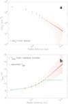Fig. 6 Density and dust temperature distributions in the core model as functions of the distance from the density peak. The squares and error bars show the mean values and standard deviations in concentric spherical shells. The assumed gas temperature profile is shown with green in the bottom panel.

Fig. 7 Predictions for the fractional oH2D+, N2H+, and DCO+ abundances as functions of the cosmic-ray ionisation rate, ${\zeta }_{{\text{H}}_2}$ (a) time, (b), and gas density (c) according to our chemistry model. The first two (a and b) represent the column density ratios N(mol)/N(H2) through the centre of the core. In panels a and c, the simulation time is 5 × 105 yr. In panels b and c, ${\zeta }_{{\text{H}}_2}={10}^{-17} {\text{s}}^{-1}$. The dashed lines in panels a and b show the fractional abundances estimated via the LTE method in Sect. 3. In panel c, higher densities are on the left to be consistent with Fig. 6.

6 Simulated line maps

The chemical abundances calculated using the one-dimensional core model at different times and for different values of the cosmic-ray ionisation rate, ${\zeta }_{{\text{H}}_2}$, were interpolated to the three-dimensional model described in Sect. 4. In the interpolation it was assumed that the abundance of a molecule depends only on the density. This means that the temperature variations in a certain density regime owing to the anisotropic external radiation field was ignored. The simulations were done using the Line radiative transfer with OpenCL (LOC) program, which uses Open Computing Language for the parallelisation of the computations (Juvela 2020). The goodness of the simulation result was evaluated by comparing the simulated integrated intensity maps with the observed ones. For this purpose, we used the image cubes from GILDAS mentioned in Sect. 3 that gave a pixel size of 5″.6. The simulated integrated intensity maps were resampled to the same grid, and the χ² statistic was evaluated over pixels where the observed integrated intensity exceeded a certain threshold. The threshold was set to 0.1 K km s⁻¹ for N₂H⁺ and DCO⁺, and 0.2 K km s⁻¹ for oH₂D⁺. This selection gave ~70−80 pixels for each map. For the σ we used the RMS integrated intensity on the outskirts of the observed maps, where the surface brightness is dominated by noise.

The best agreement between the simulated and observed integrated oH₂D⁺(1₁₀ − 1₁₁) intensity map in terms of χ² was found with ${\zeta }_{{\text{H}}_2}=5.5\times {10}^{-18} {\text{s}}^{-1}$ at the simulation time 5 × 10⁵ yr. Nearly as good agreement was obtained with ${\zeta }_{{\text{H}}_2}=7.4\times {10}^{-18} {\text{s}}^{-1}$ at 6.3 × 10⁵ yr. With the latter value of ${\zeta }_{{\text{H}}_2}$ , the agreement with the observed oH₂D⁺ map does not depend strongly on the simulation time after 6.3 × 10⁵ yr. Image-style plots of χ² as functions of ${\zeta }_{{\text{H}}_2}$ and time are shown in Fig. B.1. There we show chi-square maps for the two sets of elemental abundances mentioned in Sect. 5, and the same plot for a model with the grain radius a = 0.3 µm (instead of our standard a = 0.1 µm; see below). One can see that changes in the abundances of O, C, and N, or the assumed grain radius do not cause notable differences in the oH₂D⁺ emission.

The average fractional oH₂D⁺ abundance of the best-fit models (with ${\zeta }_{{\text{H}}_2}=(5.5-7.4)\times {10}^{-18} {\text{s}}^{-1}$) is ~2.2 × 10⁻¹⁰ towards the centre of the core, derived from column densities convolved to the angular resolution of the observations. The value is close to that estimated in Sect. 3. As can be anticipated from Fig. 7a, higher values of ${\zeta }_{{\text{H}}_2}$ produce too bright oH₂D+ lines, and for lower ${\zeta }_{{\text{H}}_2}$ the emission is weaker than observed. The ‘baseline’ model with the default elemental abundances and grain radius underpredicts the N₂H⁺(4 − 3) and the DCO⁺(5 − 4) intensities for all tested values of ${\zeta }_{{\text{H}}_2}$ at all times. Adopting the abundance profiles for the model with ${\zeta }_{{\text{H}}_2}=7.4\times {10}^{-18} {\text{s}}^{-1}$ at the time 6.3 × 10⁵ yr, but allowing the N₂H⁺ and DCO⁺ abundances to be scaled up, an approximate agreement with the observed spectra and maps is reached when the N₂H⁺ abundances are multiplied by 4.8, and the DCO⁺ abundances are multiplied by 4. With these scaling factors, the average fractional abundances towards the centre of the core are X(N₂H⁺) ~ 4.3 × 10⁻¹⁰ and X(DCO⁺) ~ 2.9 × 10⁻¹⁰ at the angular resolution of the observations. Maps and spectra towards a few selected positions calculated from the model with ${\zeta }_{{\text{H}}_2}=7.4\times {10}^{-18} {\text{s}}^{-1}$ are shown in Figs. C.1 and C.2. Here the N₂H⁺ and DCO⁺ abundances are multiplied by the factors mentioned above.

We also tested the set of higher O, C, and N abundances mentioned in Sect. 5. This did not result in significant changes in the oH₂D⁺ abundance, and for N₂H⁺ and DCO⁺ the effect is also small for low cosmic-ray ionisation rates. For ${\zeta }_{{\text{H}}_2}$ values higher than ~5 × 10⁻¹⁷ s⁻¹, the fractional DCO⁺ and N₂H⁺ abundances increase using these elemental abundances, but then the simulated intensities also remain below the observed level.

Another possible way to increase the N₂H⁺ and DCO⁺ abundances is to decrease the destruction of their precursors, N₂ and CO, through accretion onto grains. A unique grain radius of 0.1 µm assumed standardly in the present chemistry models, together with the assumed grain material density (2.5 g cm⁻³) and dust-to-gas mass ratio (0.01) imply a total surface area of dust grains of 7 × 10⁻²² cm² per H atom. Yet another series of simulations was made varying the grain radius. The tested values were 0.2 µm, 0.3 µm, and 0.4 µm. Keeping the grain material density and the dust-to-gas mass ratio constant, the total surface area is inversely proportional to a, so with the value a = 0.4 µm the grain surface area is one quarter of that in our ‘standard’ model. The N₂H⁺ abundance increased noticeably with the grain radii a = 0.2 µm and a = 0.3 µm, and decreased again with a = 0.4 µm. The observed intensity levels in the N₂H⁺ (4 − 3) map were best reproduced with the parameter values ${\zeta }_{{\text{H}}_2}=7.4\times {10}^{-18} {\text{s}}^{-1}$, a = 0.3 µm at time t = 7.9 × 10⁵ yr. For these values of ${\zeta }_{{\text{H}}_2}$ and a, the best-fit time for oH₂D⁺ is 5 × 10⁵ yr. The oH₂D⁺ abundances decrease gradually with an increasing grain radius, which must be compensated by increasing the cosmic-ray ionisation rate in order to reproduce the observed line intensities. For the grain radii a = 0.1 µm and 0.2 µm, the minimum χ² was found at ${\zeta }_{{\text{H}}_2}=5.5\times {10}^{-18} {\text{s}}^{-1}$, whereas with a = 0.3 µm and 0.4 µm, the best agreement with the oH₂D⁺ maps was achieved at ${\zeta }_{{\text{H}}_2}=7.4\times {10}^{-18} {\text{s}}^{-1}$. The DCO⁺ abundance increases when grains are made larger, and finally with a = 0.4 µm, and with a high cosmic-ray ionisation rate of ${\zeta }_{{\text{H}}_2}~{10}^{-16} {\text{s}}^{-1}$, the modelled peak intensities attain the observed values. However, cosmic-ray ionisation rates above 10⁻¹⁷ s⁻¹ are inconsistent with the oH₂D⁺ and N₂H⁺ data. The observed displacement of the DCO⁺ emission peaks from the highest densities is not reproduced by any model tested here.

Simulated oH₂D⁺, N₂H⁺, and DCO⁺ maps from the model with ${\zeta }_{{\text{H}}_2}=7.4\times {10}^{-18} {\text{s}}^{-1}$ and a = 0.3 µm are shown in Fig. D.1. Again, the DCO⁺ abundance is scaled by a factor of 4 to attain the observed peak intensity, but the oH₂D⁺ and N₂H⁺ maps are as predicted by the model, although the N₂H⁺ map represents a later simulation time (7.9 × 10⁵ yr) than the oH₂D⁺ and DCO⁺ maps (5 × 10⁵ yr).

7 Discussion

The observed oH₂D⁺ map follows the general structure of the H-MM1 core seen in the far-infrared and sub-millimetre continuum (Figs. 1 and 3). The core model misses the secondary density peak near the offset +10″, +30″ from the core centre (Fig. C.1). Besides the oH₂D⁺ and N₂H⁺ maps presented here, the presence of the secondary peak is also evident on the previous high-resolution NH₂D and NH₃ maps of the core (Harju et al. 2020; Pineda et al. 2022). According to the chemistry model, the fractional oH₂D⁺ abundance decreases typically by one order of magnitude from the outer parts to the centre of the core (Fig. 7c). For DCO⁺ and N₂H⁺, the decrease in the fractional abundance is about two orders of magnitude. Combined with the density model of the core (Fig. 6), this means that while the number densities of DCO⁺ and N₂H⁺ (cm⁻³) remain approximately constant throughout the core, the number density of oH₂D⁺ increases by a factor of 10 towards the centre. Provided that it is not optically thick, or absorbed in an ambient cloud, the oH₂D⁺(1₁₀ − 1₁₁) line is therefore a useful probe of the interior parts of dense cores. In H-MM1, we do not see signs of self-absorption in this line.

The centroid velocity and velocity dispersion maps of oH₂D⁺ shown in Fig. A.1 do not bring new information about the gas kinematics in the centre of the core. The previous maps derived from the NH₃(1,1) line observed with the VLA are superior thanks to their high spatial resolution (6″ versus 18″ achieved here) and sensitivity, despite the heavy depletion of ammonia in this region (Pineda et al. 2022). The sudden drop in the velocity dispersion seen at a declination offset of about +30″ in NH₃, DCO⁺ , and N₂H⁺ is less pronounced in oH₂D⁺ because the linewidth of this molecule is dominated by thermal motions. All three maps observed here confirm the presence of red-shifted gas in a narrow region pointing to the centre of the core. This probably represents a stream of gas falling into the centre of gravity, resembling thus larger-scale accretion streams discovered previously in association with protostars (Pineda et al. 2020; Valdivia-Mena et al. 2022, 2023). The putative stream, best discernible on the NH₃(1,1) velocity map (Fig. A.1, top-right panel), may have a role in the conception of a protostar in this core.

The shift between the DCO⁺ and H₂D⁺ maps, illustrated in Fig. 4, is reminiscent of what was seen in high-resolution maps of CH₃OH and NH₂D towards this core (Harju et al. 2020). The bright methanol emission at its shaded, eastern boundary was suggested to be caused by vigorous desorption, possibly induced by grain-grain collisions in a layer of strong velocity shear. Methanol formation requires CO-rich ice (e.g. Vasyunin et al. 2017), and carbon monoxide eventually released in this process could also have led to an intensified production of HCO⁺ and DCO⁺ . In low-mass star-forming regions, bright DCO⁺ emission sometimes marks interaction with a low-velocity outflow (Lis et al. 2016). To examine the possible connection of the methanol feature to the DCO⁺ ‘displacement’, we have overlaid in Fig. E.1 contours of strong methanol emission on the integrated intensity maps of the three lines observed here. The figure shows that the DCO⁺ peaks are not found in the direction of the brightest methanol emission, but lie west of it, slightly inwards from the core edge. The N₂H⁺ emission peak also seems to reside, at least in projection, next to methanol contours. On the whole, the differences between the distributions of DCO⁺, N₂H⁺ and oH₂D⁺ relative to CH₃OH are small. Nevertheless, the fact that DCO⁺ emission peaks on the same side of the core where most methanol is found can probably be traced to their common precursor, CO. It is possible that the distributions have been shaped by the asymmetric radiation field owing to nearby B-type stars, which has led to a measurable difference in the dust temperature between the western and eastern boundaries of the core (Harju et al. 2020, Sect. 7.1). The effects of uneven illumination on carbon chemistry and the formation of methanol in pre-stellar and starless cores have been discussed in Spezzano et al. (2016, 2020) the latter paper also presents a single-dish methanol map of H-MM1. The large-scale distribution of methanol can be understood in terms favourable conditions for the formation of CO, and CO-rich ice, on the sheltered eastern side of the core, and a relative scarcity of CO on the western side side, which is exposed to strong radiation. How these conditions influence the DCO⁺ distribution is not clear to us. The present chemistry model does not include local variations of the desorption efficiency or anisotropies of the external radiation field. This may partly explain the discrepancy between the observed and modelled DCO⁺ abundances.

The decrease in the fractional abundances of electrons and molecular ions towards higher densities predicted by the chemistry model (Fig. 7c) is a natural consequence of more frequent recombination reactions; the recombination rate (cm⁻³ s⁻¹) between molecular ions and electrons is approximately proportional to the cosmic-ray ionisation rate (here assumed to be constant) and the number density of H₂ (McKee 1989, Appendix B). For DCO⁺ and N₂H⁺ the decrease is accentuated by the disappearance of their precursors CO and N₂ owing to freezing onto dust grains. In contrast, oH₂D⁺ and the other forms of ${\text{H}}_3^{+}$ benefit from the depletion of these molecules, and the density dependence of their fractional abundance is in our model slightly shallower than ~n^−0.5 predicted by McKee (1989, see also Fig. 13 of Pineda et al. 2022).

The average oH₂D⁺ abundance is predicted to be nearly constant in time and to correlate strongly with the cosmic-ray ionisation rate (Fig. 7 a and b). The same is true for ${\text{H}}_3^{+}$ and for the combined abundance of all its modifications. In Fig. 8, we show the average fractional abundances of ${\text{H}}_3^{+}$, H₂D⁺, D₂H⁺, ${\text{D}}_3^{+}$ as functions of ${\zeta }_{{\text{H}}_2}$. The fractional abundances of the observable oH₂D⁺ and pD₂H⁺ cations are shown there with dashed red and green curves, respectively. Also shown is the total abundance of all ${\text{H}}_3^{+}$ isotopologues (cyan dashed curve; denoted $\widetilde{{\text{H}}_3^{+}}$). The fractional oH₂D⁺ abundance follows the total abundance of $\widetilde{{\text{H}}_3^{+}}$ remarkably well, at about one order of magnitude lower level. This is also true for other simulation times.

The constancy and the correlation of the average oH₂D⁺ abundance with the cosmic-ray ionisation rate is a consequence of the fact that the formation rate of ${\text{H}}_3^{+}$ is practically equal to ${\zeta }_{{\text{H}}_2}\times n\left({\text{H}}_2\right)$. The ${\text{H}}_3^{+}$ ion is deuterated through reactions with HD, starting with ${\text{H}}_3^{+}+\text{HD}\leftrightharpoons {\text{H}}_2{\text{D}}^{+}+{\text{H}}_2$. In dense gas, the fractional HD abundance is reduced slowly from the initial value ~3 × 10⁻⁵ (Sipilä et al. 2013), and deuteration is boosted when the fractional CO abundance decreases below that of HD. At high cosmic-ray ionisation rates, deuterium fractionation is, however, suppressed as ${\text{H}}_3^{+}$ is destroyed in electron recombination reactions rather than reactions with HD. In this respect, the situation resembles that in diffuse clouds. On the other hand, at low values of ${\zeta }_{{\text{H}}_2},{\text{D}}_3^{+}$ can become the dominant ion. The isotopologues of ${\text{H}}_3^{+}$ together form by far the most abundant group of cations in our core model, and the total ${\text{H}}_3^{+}$ abundance, $X\left(\widetilde{{\text{H}}_3^{+}}\right)$, is nearly equal to the electron fraction, X(e⁻). Therefore, it seems reasonable to apply the approximation presented by Watson (1976) for the minimum fractional ionisation (his Eq. (4.50)) to the total H+ abundance, and write $X\left(\widetilde{{\text{H}}_3^{+}}\right)\approx X\left({\text{e}}^{-}\right)\approx \sqrt{{\zeta }_{{\text{H}}_2}/\left(\alpha \overline{n}\left({\text{H}}_2\right)\right)}$, where a is the rate coefficient of dissociative electron recombination, and $\overline{n}\left({\text{H}}_2\right)$ is the average H₂ density. In our core model $\overline{n}\left({\text{H}}_2\right)\approx 2\times {10}^5 {\text{cm}}^{-3}$. The formula approximates the dependence of $\widetilde{{\text{H}}_3^{+}}$ on ${\zeta }_{{\text{H}}_2}$ very well in our models if we set α = 1.9 × 10⁻⁶ cm³ s⁻¹, giving $X\left(\widetilde{{\text{H}}_3^{+}}\right)\approx 1.6\sqrt{{\zeta }_{{\text{H}}_2}/{\text{s}}^{-1}}$. The α value quoted is, however, about ten times larger than typical recombination rate coefficients for ${\text{H}}_3^{+}$ and its variants at 10K (Pagani et al. 2009b; their TableB.1), and it can be thought to represent the removal of molecules from the sequence ${\text{H}}_3^{+}\leftrightharpoons {\text{H}}_2{\text{D}}^{+}\leftrightharpoons {\text{D}}_2{\text{H}}^{+}\leftrightharpoons {\text{D}}_3^{+}$ by both dissociative electron recombination (including those on grains) and proton transfer reactions, primarily to CO and N₂. Inspection of the main production and destruction pathways during the simulation reveals that at ${\zeta }_{{\text{H}}_2}={10}^{-17} {\text{s}}^{-1}$, the share of electron recombination reactions is approximately 60% of the total destruction rate of the ${\text{H}}_3^{+}$ family, whereas CO and N₂ together are responsible for about 40% of it. The relative importance of these reaction types change with ${\zeta }_{{\text{H}}_2}$, but our simulations suggest that their combined effect on $X\left(\widetilde{{\text{H}}_3^{+}}\right)$ remains approximately constant. A great majority of reactions involving the altogether nine isotopologues and spin modifications of ${\text{H}}_3^{+}$ are, however, conversions between these forms induced by HD and ortho- or para-H₂.

The cosmic-ray ionisation rate derived in H-MM1, $5\times {10}^{-18} {\text{s}}^{-1}\lesssim {\zeta }_{{\text{H}}_2}\lesssim {10}^{-17} {\text{s}}^{-1}$, is somewhat lower than previous estimates for dense clouds (1−5 × 10⁻¹⁷ s⁻¹; e.g. Dalgarno 2006; Padovani et al. 2024). Direct comparison with previous results is difficult, though, because different molecular tracers, and a number of assumptions about their abundances, have been employed (see below). Cosmic ray propagation models predict that the flux of particles responsible for H₂ ionisation is attenuated by large columns of gas (Padovani et al. 2009, 2018, 2024; Ivlev et al. 2015, 2021). According to attenuation models, ${\zeta }_{{\text{H}}_2}$ should stay above 10⁻¹⁷ s⁻¹ at column densities typical for starless dense cores (N(H₂) ~ 10²³ cm⁻², Σ ~ 0.5 g cm⁻²) (e.g. Padovani etal. 2018, their Appendix F). The upper limits for the cosmic-ray ionisation rates derived by Indriolo & McCall (2012) towards diffuse sight lines in the Ophiuchus-Scorpius region are some of the lowest in their sample, suggesting that Ophiuchus clouds may be exposed to a weaker than average cosmic ray flux (see their Sect. 6.2.4). The results presented here only pertain the local value of ${\zeta }_{{\text{H}}_2}$ in the dense core H-MM1. Our simulations with two different sets of elemental O, C, and N abundances, and different grain sizes (affecting the total surface area of grains, and thus the depletion of CO and N₂ and other molecules with heavy elements) gave similar best-fit ${\zeta }_{{\text{H}}_2}$ values, based on the agreement with the observed oH₂D⁺ abundance, which correlates strongly with ${\zeta }_{{\text{H}}_2}$. There is no such simple relationship between the cosmic-ray ionisation rate and the abundances of the two other molecules observed here. The failure to simultaneously fit the oH₂D⁺ and N₂H⁺ maps, and the underestimation of the DCO⁺ abundance are disturbing, but do not undermine the ${\zeta }_{{\text{H}}_2}$ estimate.

The problem that our chemical model underpredicts the N₂H⁺ abundance has been previously encountered by Redaelli et al. (2019, 2021) in the analysis of observations towards the pre-stellar core L1544. The improvement gained by reducing the grain surface area (end of Sect. 6) suggests that N₂ is excessively depleted in the model. Effective grain radii exceeding 0.1 µm, which were tested in Sect. 6, would imply that the dust grain size distribution is shifted towards larger grains from the classic dust model of Mathis et al. (1977), with n(a) ∝ a^−3.5 da in the range a_min = 50Å, a_max = 0.25 µm. Growth of grains to micrometre sizes owing to condensation of icy mantles and coagulation, leading to a decrease in the total surface area of the particles and hence to a lower degree of depletion, is predicted by theoretical models of gas-dust dynamics (e.g. Ossenkopf & Henning 1994; Ormel et al. 2009; Lefèvre et al. 2020; Hirashita et al. 2021). Observational evidence for the presence of large dust particles in dense cores comes from measurements of mid-infrared extinction, the discovery of scattered mid-infrared radiation, variation in the dust opacity at millimetre wavelengths, and changes in the ice band profiles in mid-infrared spectra (e.g. Steinacker et al. 2010; Chacón-Tanarro et al. 2019; Dartois et al. 2024).

To test if the derived low cosmic-ray ionisation rate can possibly be true, we made a quick calculation of the gas temperature, T_gas , in the centre of the core and at its outer edge, using the density and the dust temperature distributions of the core model shown in Fig. 6. Assuming that the line cooling rate is very low in the core centre, the cosmic-ray heating rate, Γ_cr, is approximately equal to the gas-dust energy transfer rate, Λ_gd, and adopting the expressions for these quantities from Goldsmith (2001) and Galli et al. (2002) (Eqs. (8) and (10) in the latter paper), the equilibrium T_gas corresponding to ${\zeta }_{{\text{H}}_2}=7.4\times {10}^{-18} {\text{s}}^{-1}$ is 7.2 K. Because of the strong gas-dust coupling at densities prevailing in the centre of core, Tgas would not rise much above T_dust even for substantially higher cosmic-ray ionisation rates. The value measured at the outer edge of the core is, therefore, critical. There, line cooling is important, and T_gas is obtained from the equation Γ_cr − Λ_g − Λ_gd = 0, where Λ_g is the gas cooling rate by molecular and atomic lines. Again, we adopted the parametrisation of Goldsmith (2001) for this quantity, Λ_g = α(T_gass/10 K)^β. According to our chemistry model, the fractional CO abundance at the outer edge of the core is ~6 × 10⁻⁶, which corresponds to a depletion factor (DF) of 10. Consequently, we used the values of α and β given in Table 4 of Goldsmith (2001) for model DF10, interpolated to the density n(H₂) = 2 × 10⁴ cm⁻³, characteristic of the outer edge of the core (giving α = 6 × 10⁻²⁴ ergs cm⁻³ s⁻¹ , β = 2.7). The dust temperature there is ~15 K. Substituting these numbers into the thermal balance equation one finds that T_gas = 11.2 K for ${\zeta }_{{\text{H}}_2}=7.4\times {10}^{-18} {\text{s}}^{-1}$. This agrees with the gas temperature model shown in Fig. 6, which is based on the VLA ammonia map of Pineda et al. (2022). At the outer edge, the gas is heated by dust grains (Λ_gd < 0); otherwise, the adopted ${\zeta }_{{\text{H}}_2}$ value would imply a lower gas temperature (~9.3 K, if gas-dust energy transfer would be neglected).

Finally, we briefly discuss assumptions made in analytical methods of deriving the electron abundance and the cosmic-ray ionisation from observed abundances. For a thorough analysis of these methods, we refer to Redaelli et al. (2024). The analytic methods commonly assume steady state, and derive the abundance of the dominant ion, ${\text{H}}_3^{+}$, from that of an abundant observable ion, such as HCO⁺ or oH₂D⁺. Here, one has to consider the importance of proton transfer reactions (for example, ${\text{H}}_3^{+}+\text{CO}\to {\text{HCO}}^{+}+{\text{H}}_2$) relative to the dissociative electron recombination (${\text{H}}_3^{+}+{\text{e}}^{-}\to {\text{H}}_2+\text{H}$) in the destruction of ${\text{H}}_3^{+}$ (or its deuterated forms). When high densities are concerned, a proper judgement on this issue would require modelling. If oH₂D⁺ or pD₂H⁺ are used as substitutes of ${\text{H}}_3^{+}$, the difficulty is that neither the ortho/para ratios of these molecules nor the fractionation ratios ${\text{H}}_2{\text{D}}^{+}/{\text{H}}_3^{+}$ and ${\text{D}}_2{\text{H}}^{+}/{\text{H}}_3^{+}$ are known a priori (Fig. 8). A common assumption is that DCO⁺/HCO⁺ and N₂D⁺ /N²H⁺ are $~1/3\times {\text{H}}_2{\text{D}}^{+}/{\text{H}}_3^{+}$. This is based on the idea that H₂D⁺ is the principal deuterated form of ${\text{H}}_3^{+}$, and that one third of the reactions CO + H₂D⁺ and N₂ + H₂D⁺ leads to DCO⁺ and N₂D⁺, respectively. The fact that D₂H⁺ and ${\text{D}}_3^{+}$ also contribute to the formation of DCO⁺ and N₂D⁺ is taken into account in the steady-state formula for the fractionation ratios N₂D⁺/N₂H⁺ and DCO⁺ /HCO⁺ presented by Caselli et al. (2008) and Pagani et al. (2009b) (their Eqs. (13) and (10), respectively): $$\frac{{\text{N}}_2{\text{D}}^{+}}{{\text{N}}_2{\text{H}}^{+}}\approx \frac{{\text{DCO}}^{+}}{{\text{HCO}}^{+}}\approx \frac{{\text{H}}_2{\text{D}}^{+}+2{\text{D}}_2{\text{H}}^{+}+3{\text{D}}_3^{+}}{3{\text{H}}_3^{+}+2{\text{H}}_2{\text{D}}^{+}+{\text{D}}_2{\text{H}}^{+}}.$$

In Fig. F.1, we show the ratios N₂D⁺/N₂H⁺ and DCO⁺ /HCO⁺ from our models as functions of the cosmic-ray ionisation rate and time, along with the prediction from the equation above. Also shown is the ratio $1/3\times {\text{H}}_2{\text{D}}^{+}/{\text{H}}_3^{+}$, which often is assumed to be equal to DCO⁺/HCO⁺ or N₂D⁺/N₂H⁺. Besides the model with the fiducial set of parameters, diagrams are shown for the model with the grain radius a = 0.3 µm, which can approximately reproduce both oH₂D⁺ and N₂H⁺ intensities. While the steady-state formula shown above gives a nearly perfect match, one can see that the DCO⁺/HCO⁺ and N₂D⁺/N₂H⁺ ratios do not serve as good templates of the quantity $1/3\times {\text{H}}_2{\text{D}}^{+}/{\text{H}}_3^{+}$ in this case. The discrepancy is a factor of 2–3, and thus still within the estimated accuracy of the common approximation according to Redaelli et al. (2024). For targets with lower average densities the agreement is probably better. Unfortunately, the present observations do not include HCO⁺ or N₂D⁺ lines to test the predictions for the fractionation ratios.

Fig. 8 Average fractional abundances of ${\text{H}}_3^{+}$, its deuterated isotopo-logues, and electrons in the core model as functions of the cosmic-ray ionisation rate, ${\zeta }_{{\text{H}}_2}$. The solid red curve shows the total (ortho + para) abundance of H2D+, whereas the dashed red curve shows the fractional oH2D+ abundance separately. Likewise, the dashed green curve shows the fractional pD2H+ abundance. The combined fractional abundance of all modifications of ${\text{H}}_3^{+}$, denoted $\widetilde{{\text{H}}_3^{+}}$ in the text, is shown with the dashed cyan curve.

8 Conclusions

Each of the three common molecular ions, oH₂D⁺, N₂H⁺, and DCO⁺, presents a different picture of the pre-stellar core H-MM1. The oH₂D⁺(1₁₀−1₁₁⁾ emission closely follows the general structure of the core seen in the far-infrared and in ammonia maps. The line is already excited at densities around 10⁵ cm⁻³, but its optical thickness remains moderate towards the densest regions, partly because of the broad thermal linewidth and the hyperfine structure. The N₂H⁺(4 − 3) emission is more compact, concentrating on the density maxima. Like N₂H⁺(4 − 3), the DCO⁺(5 − 4) line has a high critical density, but its emission maxima are shifted eastwards from the density peaks, towards the more sheltered side of the core.

The chemistry model used to interpret the observed map highlights two advantages of oH₂D⁺ observations: (1) the fractional oH₂D⁺ abundance also remains relatively high in the interiors of the core, where N₂H⁺ and DCO⁺ are depleted by a factor of 100 or more; and (2) the average oH₂D⁺ abundance is nearly constant in time, and correlates strongly with the cosmic-ray ionisation rate owing to its direct relationship to the primary ionisation product, ${\text{H}}_3^{+}$. The observed oH₂D⁺ line emission constrains the cosmic-ray ionisation rate to ${\zeta }_{{\text{H}}_2}~5\times {10}^{-18} {\text{s}}^{-1}-1\times {10}^{-17} {\text{s}}^{-1}$. A substantial increase in the assumed elemental O, C, and N abundances, or a decrease in the total surface area of the dust grains in the chemistry model, does not change the best-fit ${\zeta }_{{\text{H}}_2}$ value markedly, and the estimate ${\zeta }_{{\text{H}}_2}\lesssim {10}^{-17} {\text{s}}^{-1}$ in H-MM1 seems robust. The estimate is further supported by the low gas temperature measured on the outskirts of the core. The H₂ column density of the ambient cloud around the core is of the order of 10²² cm⁻², and the low ${\zeta }_{{\text{H}}_2}$ value derived in H-MM1 compared with estimates in diffuse clouds can probably be understood in terms of attenuation of the cosmic ray flux in dense gas (e.g. Padovani et al. 2018), although propagation models predict higher ionisation rates at this column density. Our modelling results corroborate the conclusion from the analysis presented in Bovino et al. (2020) and Redaelli et al. (2024), that oH₂D⁺ observations are useful for deriving the cosmic-ray ionisation rate in dense dark clouds where ${\text{H}}_3^{+}$ is not observable. However, the oH₂D⁺ abundance relative to that of ${\text{H}}_3^{+}$ cannot be reliably obtained from the observable fractionation ratios DCO⁺/HCO⁺ and N₂D⁺/N₂H⁺. Modelling the oH₂D⁺ line emission using ${\zeta }_{{\text{H}}_2}$ as a parameter provides a more straightforward method.

Acknowledgements

We thank the APEX staff for performing the observations presented here, and the referee for helpful suggestions to improve the manuscript. The authors gratefully acknowledge financial support from the Max Planck Society.

Appendix A Radial velocity and velocity dispersion maps

The distributions of the centroid LSR velocities and the line-of-sight velocity dispersions of the observed lines in H-MM1 are shown in Fig. A.1. The points with high signal-to-noise ratios are selected to these images. In addition to maps derived from the oH₂D⁺, N₂H⁺, and DCO⁺ lines, the centroid V_LSR and σ_V distributions of the NH₃(1,1) line from the VLA mapping of Pineda et al. (2022) are shown, resampled to the grid used for the present LAsMA observations.

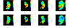Fig. A.1 Distributions of the centroid LSR velocities and velocity dispersions of the lines observed towards H-MM1. Points with low signal-to-noise ratios are excluded. The right hand panel shows results from the VLA NH3 mapping by Pineda et al. (2022), resampled to the grid used for the LAsMA maps.

Appendix B Fitting the cosmic-ray ionisation rate

The cosmic-ray ionisation rate in the core is estimated by comparing the simulated integrated intensity maps to those observed as described in Sect. 6. Figure B.1 shows the chi-square distributions as functions of time and ${\zeta }_{{\text{H}}_2}$ for chemistry models assuming either different elemental abundances or different dust grain radii. The pixelation reflects the discrete sets of simulation times and ${\zeta }_{{\text{H}}_2}$ values tested.

Fig. B.1 Chi-square maps from comparison between the observed and simulated oH2D+ integrated intensity maps described in Sect. 6. The y-axis in the plots is the logarithm of the cosmic-ray ionisation rate, ${\zeta }_{{\text{H}}_2}$, and the x-axis is logarithm of time. The χ2 values are also presented on a logarithmic scale: a darker shade means a better fit. The plot on the left (a) represents simulations with the grain radius a = 0.1 µm and low elemental abundances of O, C, and N, assumed in several previous models of H-MM1, and that in the middle (b) simulations with some 40%–60% higher elemental O, C, and N abundances. The chi-square map on the right (c), is from a simulation with the grain radius a = 0.3 µm and low O, C, and N abundances (see Sect. 5).

Appendix C Modelled maps and spectra

The integrated intensity maps of the oH₂D⁺ (1₁₀ − 1₁₁) N₂H⁺ (4 − 3), and DCO⁺ (5 − 4) lines towards H-MM1 and the corresponding simulated maps from a three-dimensional model of the core are shown in Fig. C.1. Observed and simulated spectra in selected core positions are shown in Fig. C.2.

Fig. C.1 Observed (left) and modelled (right) integrated intensity maps of H-MM1 in oH2D+ (110 − 111) (top), N2H+ (4 − 3) (middle), and DCO+ (5 − 4) (bottom). The model assumes a cosmic-ray ionisation rate per H2 molecule of ${\zeta }_{{\text{H}}_2}=7.4\times {10}^{-18} {\text{s}}^{-1}$. The simulation time is 6.3 × 105 yr. The oH2D+ map is as predicted by the model, whereas the modelled abundances of N2H+ and DCO+ are multiplied by 4.8 and 4, respectively, to reproduce the observed intensity levels. The intensity scale is $T_{\text{A}}^{*}$. The colour scales and the contours are the same as in Fig. 3. The squares indicate positions from which the spectra shown in Fig. C.2 are extracted.

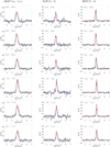Fig. C.2 Observed and modelled oH2D+(110 − 111) (left), N2H+(4 − 3) (middle), and DCO+(5 − 4) (right) spectra towards selected positions in H-MM1. The positions are indicated with square markers on the maps in Fig. C.1. The model spectra are shown in red. The offsets are with respect to the column density peak of the core. The model is the same as in Fig. C.1, and the scaling factors of the N2H+ and DCO+ abundances are also the same. The intensity scale is $T_{\text{A}}^{*}$.

Appendix D Simulated maps from the model with a larger grain size

The integrated intensity maps calculated from the model with the grain radius a = 0.3 µm are shown in Fig. D.1. The oH₂D⁺(1₁₀ −1₁₁) and N₂H⁺(4 − 3) maps are as predicted by the model, but the fractional DCO⁺ abundance is multiplied by four to achieve the observed peak intensity of the J = 5 − 4 line. Moreover, the simulated H₂D⁺ (1₁₀ − 1₁₁) and N₂H⁺(4 − 3) maps did not agree with the observations at the same time, and the N₂H⁺ map represents a later stage of evolution.

Fig. D.1 Integrated oH2D+(110 − 111) N2H+(4 − 3), and DCO+(5 − 4) maps from a model where the grain radius is assumed to be a = 0.3 µm. This model approximately reproduces the observed oH2D+ and N2H+ line intensities but underpredicts the DCO+ intensity. In the core model shown in the figure, the fractional DCO+ abundance is multiplied by 4. The simulation times are shown in the titles of the images.

Appendix E Comparison with the methanol map

The distribution of strong methanol emission observed with ALMA is shown as contour plots on the oH₂D⁺, N₂H⁺, and DCO⁺ maps in Fig. E.1. The methanol data are from Harju et al. (2020).

Fig. E.1 Integrated CH3OH(2k − 1k) line intensity contours superimposed on the oH2D+(110 −111) N2H+(4 − 3), and DCO+(5 − 4) maps of H-MM1. The contour levels are 2, 3, and 4 K km s−1 (on the TB scale). The methanol observations at 96.7 GHz are from ALMA and have an angular resolution of 4″. The colour scales of the pixel images are the same as in Fig. 3. The APEX and ALMA beams are shown in the bottom right.

Appendix F Predicted fractionation ratios

The modelled fractionation ratios DCO⁺/HCO⁺ and N₂D⁺/N₂H⁺ as functions of the cosmic-ray ionisation rate ${\zeta }_{{\text{H}}_2}$ and the simulation time are shown in Fig. F.1, together with the prediction from the steady-state formula accounting for multiply deuterated forms of ${\text{H}}_3^{+}$ (Caselli et al. 2008; Pagani et al. 2009b; see Sect. 7). Also shown is the ratio $1/3\times {\text{H}}_2{\text{D}}^{+}/{\text{H}}_3^{+}$, which is often assumed to be equal to DCO⁺/HCO⁺ or N₂D⁺/N₂H⁺ in analytical methods of deriving ${\zeta }_{{\text{H}}_2}$. The quantities presented in the figure are column density ratios along the line of sight going through the core centre. The diagrams are shown for two models: one assuming a unique grain radius of a = 0.1 µm and another assuming a = 0.3 µm.

Fig. F.1 Fractionation ratios DCO+/HCO+ and N2D+/N2H+ as functions of ${\zeta }_{{\text{H}}_2}$ (left) and time (right) according to our chemistry model. The upper row (a and b) corresponds to a model with the grain radius a = 0.1 µm, whereas the simulation used for the bottom row (c and d) assumes a = 0.3 µm. The cyan curve shows the prediction from a steady-state formula derived for a chemical network that includes multiply deuterated forms (see Sect. 7). The dashed red curve shows the ratio $1/3\times {\text{H}}_2{\text{D}}^{+}/{\text{H}}_3^{+}$.

References

All Tables

All Figures

Fig. 1 H2 column density and dust colour temperature (TC) maps of H-MM1 derived from Herschel-SPIRE HiRes data. The rectangle shows the area covered by the grid used for the line maps derived from the OTF observations. The circle shows the effective beam size (FWHM) of the SPIRE HiRes maps at 500 µm. The plus sign shows the location of the H2 column density peak of the core, used as (0,0) in the molecular line maps.

In the text

	Fig. 2 oH2D+ (110 − In), N2H+ (4 − 3), and DCO+ (5 − 4) spectra towards the density peak of the core. The red bars indicate the hyperfine structure components of the line.
In the text

	Fig. 3 Integrated oH2D+ (110 − N2H+ (4 − 3), and DCO+ (5 − 4) line intensity maps of H-MM1. The contours are: 0.10 to 0.25 by 0.03 K km s−1 (oH2D+); 0.06 to 0.14 by 0.02 K km s−1 (N2H+ ); and 0.05 to 0.11 by 0.02 K km s−1 (DCO+). The intensity scale is $T_{\text{A}}^{*}$.
In the text

	Fig. 4 Integrated oH2D+ (110 − 111) line intensity maps of H-MM1 with the DCO+ (5 − 4) contours superposed. The contour levels are the same as in Fig. 3.
In the text

	Fig. 5 H2 column density map of H-MM1 derived by combining the 8 µm surface brightness map observed with Spitzer with SPIRE HiRes far-infrared maps. The angular resolution is 6″ in the central parts of the map, and 15″ on the outskirts. The effective beam sizes are shown in the bottom-right corner. The box shows the region covered by the molecular line maps.
In the text

	Fig. 6 Density and dust temperature distributions in the core model as functions of the distance from the density peak. The squares and error bars show the mean values and standard deviations in concentric spherical shells. The assumed gas temperature profile is shown with green in the bottom panel.
In the text

Fig. 7 Predictions for the fractional oH2D+, N2H+, and DCO+ abundances as functions of the cosmic-ray ionisation rate, ${\zeta }_{{\text{H}}_2}$ (a) time, (b), and gas density (c) according to our chemistry model. The first two (a and b) represent the column density ratios N(mol)/N(H2) through the centre of the core. In panels a and c, the simulation time is 5 × 105 yr. In panels b and c, ${\zeta }_{{\text{H}}_2}={10}^{-17} {\text{s}}^{-1}$. The dashed lines in panels a and b show the fractional abundances estimated via the LTE method in Sect. 3. In panel c, higher densities are on the left to be consistent with Fig. 6.

In the text

Fig. 8 Average fractional abundances of ${\text{H}}_3^{+}$, its deuterated isotopo-logues, and electrons in the core model as functions of the cosmic-ray ionisation rate, ${\zeta }_{{\text{H}}_2}$. The solid red curve shows the total (ortho + para) abundance of H2D+, whereas the dashed red curve shows the fractional oH2D+ abundance separately. Likewise, the dashed green curve shows the fractional pD2H+ abundance. The combined fractional abundance of all modifications of ${\text{H}}_3^{+}$, denoted $\widetilde{{\text{H}}_3^{+}}$ in the text, is shown with the dashed cyan curve.

In the text

	Fig. A.1 Distributions of the centroid LSR velocities and velocity dispersions of the lines observed towards H-MM1. Points with low signal-to-noise ratios are excluded. The right hand panel shows results from the VLA NH3 mapping by Pineda et al. (2022), resampled to the grid used for the LAsMA maps.
In the text

Fig. B.1 Chi-square maps from comparison between the observed and simulated oH2D+ integrated intensity maps described in Sect. 6. The y-axis in the plots is the logarithm of the cosmic-ray ionisation rate, ${\zeta }_{{\text{H}}_2}$, and the x-axis is logarithm of time. The χ2 values are also presented on a logarithmic scale: a darker shade means a better fit. The plot on the left (a) represents simulations with the grain radius a = 0.1 µm and low elemental abundances of O, C, and N, assumed in several previous models of H-MM1, and that in the middle (b) simulations with some 40%–60% higher elemental O, C, and N abundances. The chi-square map on the right (c), is from a simulation with the grain radius a = 0.3 µm and low O, C, and N abundances (see Sect. 5).

In the text

Fig. C.1 Observed (left) and modelled (right) integrated intensity maps of H-MM1 in oH2D+ (110 − 111) (top), N2H+ (4 − 3) (middle), and DCO+ (5 − 4) (bottom). The model assumes a cosmic-ray ionisation rate per H2 molecule of ${\zeta }_{{\text{H}}_2}=7.4\times {10}^{-18} {\text{s}}^{-1}$. The simulation time is 6.3 × 105 yr. The oH2D+ map is as predicted by the model, whereas the modelled abundances of N2H+ and DCO+ are multiplied by 4.8 and 4, respectively, to reproduce the observed intensity levels. The intensity scale is $T_{\text{A}}^{*}$. The colour scales and the contours are the same as in Fig. 3. The squares indicate positions from which the spectra shown in Fig. C.2 are extracted.

In the text

Fig. C.2 Observed and modelled oH2D+(110 − 111) (left), N2H+(4 − 3) (middle), and DCO+(5 − 4) (right) spectra towards selected positions in H-MM1. The positions are indicated with square markers on the maps in Fig. C.1. The model spectra are shown in red. The offsets are with respect to the column density peak of the core. The model is the same as in Fig. C.1, and the scaling factors of the N2H+ and DCO+ abundances are also the same. The intensity scale is $T_{\text{A}}^{*}$.

In the text

Fig. D.1 Integrated oH2D+(110 − 111) N2H+(4 − 3), and DCO+(5 − 4) maps from a model where the grain radius is assumed to be a = 0.3 µm. This model approximately reproduces the observed oH2D+ and N2H+ line intensities but underpredicts the DCO+ intensity. In the core model shown in the figure, the fractional DCO+ abundance is multiplied by 4. The simulation times are shown in the titles of the images.

In the text

Fig. E.1 Integrated CH3OH(2k − 1k) line intensity contours superimposed on the oH2D+(110 −111) N2H+(4 − 3), and DCO+(5 − 4) maps of H-MM1. The contour levels are 2, 3, and 4 K km s−1 (on the TB scale). The methanol observations at 96.7 GHz are from ALMA and have an angular resolution of 4″. The colour scales of the pixel images are the same as in Fig. 3. The APEX and ALMA beams are shown in the bottom right.

In the text

Fig. F.1 Fractionation ratios DCO+/HCO+ and N2D+/N2H+ as functions of ${\zeta }_{{\text{H}}_2}$ (left) and time (right) according to our chemistry model. The upper row (a and b) corresponds to a model with the grain radius a = 0.1 µm, whereas the simulation used for the bottom row (c and d) assumes a = 0.3 µm. The cyan curve shows the prediction from a steady-state formula derived for a chemical network that includes multiply deuterated forms (see Sect. 7). The dashed red curve shows the ratio $1/3\times {\text{H}}_2{\text{D}}^{+}/{\text{H}}_3^{+}$.

In the text

References

- Arzoumanian, D., André, P., Didelon, P., et al. 2011, A&A, 529, A6 [Google Scholar]
- Bovino, S., Ferrada-Chamorro, S., Lupi, A., Schleicher, D. R. G., & Caselli, P. 2020, MNRAS, 495, L7 [Google Scholar]
- Burke, J. R., & Hollenbach, D. J. 1983, ApJ, 265, 223 [NASA ADS] [CrossRef] [Google Scholar]
- Caselli, P., & Dore, L. 2005, A&A, 433, 1145 [NASA ADS] [CrossRef] [EDP Sciences] [Google Scholar]
- Caselli, P., Walmsley, C. M., Terzieva, R., & Herbst, E. 1998, ApJ, 499, 234 [Google Scholar]
- Caselli, P., Walmsley, C. M., Zucconi, A., et al. 2002, ApJ, 565, 344 [Google Scholar]
- Caselli, P., van der Tak, F. F. S., Ceccarelli, C., & Bacmann, A. 2003, A&A, 403, L37 [CrossRef] [EDP Sciences] [Google Scholar]
- Caselli, P., Vastel, C., Ceccarelli, C., et al. 2008, A&A, 492, 703 [NASA ADS] [CrossRef] [EDP Sciences] [Google Scholar]
- Chacón-Tanarro, A., Pineda, J. E., Caselli, P., et al. 2019, A&A, 623, A118 [NASA ADS] [CrossRef] [EDP Sciences] [Google Scholar]
- Dalgarno, A. 2006, PNAS, 103, 12269 [NASA ADS] [CrossRef] [Google Scholar]
- Dartois, E., Noble, J. A., Caselli, P., et al. 2024, Nat. Astron., 8, 359 [NASA ADS] [CrossRef] [Google Scholar]
- Denis-Alpizar, O., Stoecklin, T., Dutrey, A., & Guilloteau, S. 2020, MNRAS, 497, 4276 [Google Scholar]
- Galli, D., & Padovani, M. 2015, arXiv e-prints [arXiv:1502.03380] [Google Scholar]
- Galli, D., Walmsley, M., & Gonçalves, J. 2002, A&A, 394, 275 [NASA ADS] [CrossRef] [EDP Sciences] [Google Scholar]
- Goldsmith, P. F. 2001, ApJ, 557, 736 [Google Scholar]
- Griffin, M. J., Abergel, A., Abreu, A., et al. 2010, A&A, 518, A3 [Google Scholar]
- Guelin, M., Langer, W. D., Snell, R. L., & Wootten, H. A. 1977, ApJ, 217, L165 [NASA ADS] [CrossRef] [Google Scholar]
- Harju, J., Daniel, F., Sipilä, O., et al. 2017, A&A, 600, A61 [NASA ADS] [CrossRef] [EDP Sciences] [Google Scholar]
- Harju, J., Pineda, J. E., Vasyunin, A. I., et al. 2020, ApJ, 895, 101 [NASA ADS] [CrossRef] [Google Scholar]
- Harju, J., Pineda, J. E., Sipilä, O., et al. 2024, A&A, 682, A8 [NASA ADS] [CrossRef] [EDP Sciences] [Google Scholar]
- Hirashita, H., Il’in, V. B., Pagani, L., & Lefèvre, C. 2021, MNRAS, 502, 15 [NASA ADS] [CrossRef] [Google Scholar]
- Hugo, E., Asvany, O., & Schlemmer, S. 2009, J. Chem. Phys., 130, 164302 [Google Scholar]
- Indriolo, N., & McCall, B. J. 2012, ApJ, 745, 91 [NASA ADS] [CrossRef] [Google Scholar]
- Ivlev, A. V., Padovani, M., Galli, D., & Caselli, P. 2015, ApJ, 812, 135 [Google Scholar]
- Ivlev, A. V., Silsbee, K., Sipilä, O., & Caselli, P. 2019, ApJ, 884, 176 [Google Scholar]
- Ivlev, A. V., Silsbee, K., Padovani, M., & Galli, D. 2021, ApJ, 909, 107 [NASA ADS] [CrossRef] [Google Scholar]
- Jensen, P., Paidarova, I., Spirko, V., & Sauer, S. P. A. 1997, Mol. Phys., 91, 319 [NASA ADS] [Google Scholar]
- Jusko, P., Töpfer, M., Müller, H. S. P., et al. 2017, J. Mol. Spectrosc., 332, 33 [NASA ADS] [CrossRef] [Google Scholar]
- Juvela, M. 2020, A&A, 644, A151 [NASA ADS] [CrossRef] [EDP Sciences] [Google Scholar]
- Lattanzi, V., Walters, A., Drouin, B. J., & Pearson, J. C. 2007, ApJ, 662, 771 [NASA ADS] [CrossRef] [Google Scholar]
- Lefèvre, C., Pagani, L., Ladjelate, B., et al. 2020, in Eur. Phys. J. Web Conf., 228, mm Universe @ NIKA2 – Observing the mm Universe with the NIKA2 Camera, 00013 [Google Scholar]
- Lis, D. C., Wootten, H. A., Gerin, M., et al. 2016, ApJ, 827, 133 [NASA ADS] [CrossRef] [Google Scholar]
- Mangum, J. G., Emerson, D. T., & Greisen, E. W. 2007, A&A, 474, 679 [NASA ADS] [CrossRef] [EDP Sciences] [Google Scholar]
- Mathis, J. S., Rumpl, W., & Nordsieck, K. H. 1977, ApJ, 217, 425 [Google Scholar]
- McKee, C. F. 1989, ApJ, 345, 782 [NASA ADS] [CrossRef] [Google Scholar]
- Neufeld, D. A., & Wolfire, M. G. 2017, ApJ, 845, 163 [Google Scholar]
- Ormel, C. W., Paszun, D., Dominik, C., & Tielens, A. G. G. M. 2009, A&A, 502, 845 [NASA ADS] [CrossRef] [EDP Sciences] [Google Scholar]
- Ossenkopf, V., & Henning, T. 1994, A&A, 291, 943 [NASA ADS] [Google Scholar]
- Padovani, M., Galli, D., & Glassgold, A. E. 2009, A&A, 501, 619 [NASA ADS] [CrossRef] [EDP Sciences] [Google Scholar]
- Padovani, M., Ivlev, A. V., Galli, D., & Caselli, P. 2018, A&A, 614, A111 [NASA ADS] [CrossRef] [EDP Sciences] [Google Scholar]
- Padovani, M., Ivlev, A. V., Galli, D., et al. 2020, Space Sci. Rev., 216, 29 [CrossRef] [Google Scholar]
- Padovani, M., Galli, D., Scarlett, L. H., et al. 2024, A&A, 682, A131 [NASA ADS] [CrossRef] [EDP Sciences] [Google Scholar]
- Pagani, L., Daniel, F., & Dubernet, M. L. 2009a, A&A, 494, 719 [NASA ADS] [CrossRef] [EDP Sciences] [Google Scholar]
- Pagani, L., Vastel, C., Hugo, E., et al. 2009b, A&A, 494, 623 [NASA ADS] [CrossRef] [EDP Sciences] [Google Scholar]
- Parise, B., Belloche, A., Du, F., Güsten, R., & Menten, K. M. 2011, A&A, 526, A31 [NASA ADS] [CrossRef] [EDP Sciences] [Google Scholar]
- Pineda, J. E., Segura-Cox, D., Caselli, P., et al. 2020, Nat. Astron., 4, 1158 [NASA ADS] [CrossRef] [Google Scholar]
- Pineda, J. E., Harju, J., Caselli, P., et al. 2022, AJ, 163, 294 [NASA ADS] [CrossRef] [Google Scholar]
- Redaelli, E., Bizzocchi, L., Caselli, P., et al. 2019, A&A, 629, A15 [NASA ADS] [CrossRef] [EDP Sciences] [Google Scholar]
- Redaelli, E., Sipilä, O., Padovani, M., et al. 2021, A&A, 656, A109 [NASA ADS] [CrossRef] [EDP Sciences] [Google Scholar]
- Redaelli, E., Bovino, S., Lupi, A., et al. 2024, A&A, 685, A67 [NASA ADS] [CrossRef] [EDP Sciences] [Google Scholar]
- Riedel, W., Sipilä, O., Redaelli, E., et al. 2023, A&A, 680, A87 [NASA ADS] [CrossRef] [EDP Sciences] [Google Scholar]
- Roberts, H., Herbst, E., & Millar, T. J. 2003, ApJ, 591, L41 [CrossRef] [Google Scholar]
- Sabatini, G., Bovino, S., & Redaelli, E. 2023, ApJ, 947, L18 [NASA ADS] [CrossRef] [Google Scholar]
- Sawada, T., Ikeda, N., Sunada, K., et al. 2008, PASJ, 60, 445 [NASA ADS] [Google Scholar]
- Schöier, F. L., van der Tak, F. F. S., van Dishoeck, E. F., & Black, J. H. 2005, A&A, 432, 369 [Google Scholar]
- Shirley, Y. L. 2015, PASP, 127, 299 [Google Scholar]
- Sipilä, O., Caselli, P., & Harju, J. 2013, A&A, 554, A92 [NASA ADS] [CrossRef] [EDP Sciences] [Google Scholar]
- Sipilä, O., Caselli, P., & Harju, J. 2019, A&A, 631, A63 [Google Scholar]
- Sipilä, O., Caselli, P., Redaelli, E., & Spezzano, S. 2022, A&A, 668, A131 [NASA ADS] [CrossRef] [EDP Sciences] [Google Scholar]
- Spezzano, S., Bizzocchi, L., Caselli, P., Harju, J., & Brünken, S. 2016, A&A, 592, L11 [NASA ADS] [CrossRef] [EDP Sciences] [Google Scholar]
- Spezzano, S., Caselli, P., Pineda, J. E., et al. 2020, A&A, 643, A60 [NASA ADS] [CrossRef] [EDP Sciences] [Google Scholar]
- Steinacker, J., Pagani, L., Bacmann, A., & Guieu, S. 2010, A&A, 511, A9 [NASA ADS] [CrossRef] [EDP Sciences] [Google Scholar]
- Valdivia-Mena, M. T., Pineda, J. E., Segura-Cox, D. M., et al. 2022, A&A, 667, A12 [NASA ADS] [CrossRef] [EDP Sciences] [Google Scholar]
- Valdivia-Mena, M. T., Pineda, J. E., Segura-Cox, D. M., et al. 2023, A&A, 677, A92 [NASA ADS] [CrossRef] [EDP Sciences] [Google Scholar]
- van der Tak, F. F. S. & van Dishoeck, E. F. 2000, A&A, 358, L79 [NASA ADS] [Google Scholar]
- Vastel, C., Phillips, T. G., & Yoshida, H. 2004, ApJ, 606, L127 [Google Scholar]
- Vastel, C., Caselli, P., Ceccarelli, C., et al. 2006a, ApJ, 645, 1198 [NASA ADS] [CrossRef] [Google Scholar]
- Vastel, C., Phillips, T. G., Caselli, P., Ceccarelli, C., & Pagani, L. 2006b, Philos. Trans. Roy. Soc. London Ser. A, 364, 3081 [NASA ADS] [Google Scholar]
- Vasyunin, A. I., Caselli, P., Dulieu, F., & Jiménez-Serra, I. 2017, ApJ, 842, 33 [Google Scholar]
- Walmsley, C. M., Flower, D. R., & Pineau des Forêts, G. 2004, A&A, 418, 1035 [NASA ADS] [CrossRef] [EDP Sciences] [Google Scholar]
- Watson, W. D. 1976, Rev. Mod. Phys., 48, 513 [NASA ADS] [CrossRef] [Google Scholar]
- Wootten, A., Snell, R., & Glassgold, A. E. 1979, ApJ, 234, 876 [NASA ADS] [CrossRef] [Google Scholar]