| Issue |
A&A
Volume 688, August 2024
|
|
|---|---|---|
| Article Number | A118 | |
| Number of page(s) | 22 | |
| Section | Interstellar and circumstellar matter | |
| DOI | https://doi.org/10.1051/0004-6361/202348529 | |
| Published online | 13 August 2024 | |
Deuterium fractionation of the starless core L 1498★
1
Academia Sinica Institute of Astronomy and Astrophysics (ASIAA),
No. 1, Section 4, Roosevelt Road,
Taipei
10617,
Taiwan
e-mail: This email address is being protected from spambots. You need JavaScript enabled to view it.
2
Institute of Astronomy, National Tsing Hua University (NTHU),
No. 101, Section 2, Kuang-Fu Road,
Hsinchu
30013,
Taiwan
3
Center for Informatics and Computation in Astronomy (CICA),
NTHU, No. 101, Section 2, Kuang-Fu Road,
Hsinchu
30013,
Taiwan
e-mail: This email address is being protected from spambots. You need JavaScript enabled to view it.
4
LERMA & UMR8112 du CNRS, Observatoire de Paris, PSL University, Sorbonne Universités, CNRS,
75014
Paris,
France
5
Institut de Radioastronomie Millimétrique (IRAM),
300 rue de la Piscine,
38400
Saint-Martin-d’Hères,
France
Received:
9
November
2023
Accepted:
21
May
2024
Abstract
Context. Molecular deuteration is commonly seen in starless cores and is expected to occur on a timescale comparable to that of the core contraction. Thus, the deuteration serves as a chemical clock, allowing us to investigate dynamical theories of core formation.
Aims. We aim to provide a 3D cloud description for the starless core L 1498 located in the nearby low-mass star-forming region Taurus and explore its possible core formation mechanism.
Methods. We carried out nonlocal thermal equilibrium radiative transfer with multi-transition observations of the high-density tracer N2H+ to derive the density and temperature profiles of the L 1498 core. By combining these observations with the spectral observations of the deuterated species, ortho-H2D+, N2D+, and DCO+, we derived the abundance profiles for the observed species and performed chemical modeling of the deuteration profiles across L 1498 to constrain the contraction timescale.
Results. We present the first ortho-H2D+ (110−111) detection toward L 1498. We find a peak molecular hydrogen density of 1.6−0.3+3.0 × 105 cm−3, a temperature of 7.5−0.5+0.7 K, and a N2H+ deuteration of 0.27−0.15+0.12 in the center.
Conclusions. We derived a lower limit of the core age for L 1498 of 0.16 Ma, which is compatible with the typical free-fall time, indicating that L 1498 likely formed rapidly.
Key words: ISM: abundances / ISM: clouds / ISM: kinematics and dynamics / ISM: structure / ISM: individual objects: LDN 1498
Publisher note: A missing grant number was added on 30 August 2024.
The reduced CFHT J, H, Ks-band images are available at the CDS via anonymous ftp to cdsarc.cds.unistra.fr (130.79.128.5) or via https://cdsarc.cds.unistra.fr/viz-bin/cat/J/A+A/688/A118
© The Authors 2024
 Open Access article, published by EDP Sciences, under the terms of the Creative Commons Attribution License (https://creativecommons.org/licenses/by/4.0), which permits unrestricted use, distribution, and reproduction in any medium, provided the original work is properly cited.
This article is published in open access under the Subscribe to Open model. This email address is being protected from spambots. You need JavaScript enabled to view it. to support open access publication.
1 Introduction
Deuterium fractionation is closely related to star formation. Almost all deuterium was formed through primordial nucleosynthesis after the birth of the Universe, and there is no other process significantly producing deuterium afterward (Wannier 1980). The atomic deuterium fraction (D/H) is measured as 1.6×10⁻⁵ in the Local Bubble (Linsky 2007). In dark clouds, hydrogen primarily exists in its molecular form, and HD serves as the primary deuterium reservoir, inheriting the deuterium fraction as 3.2 × 10⁻⁵. However, deuterium fractionation in other hydrogen-containing molecules is found to be enhanced by several orders of magnitude in star-forming regions, especially, in starless cores (Ceccarelli et al. 2014).
Starless cores are the potential birthplaces of future stars and planets, where the key species leading the deuterium fractionation is trihydrogen cation,  . The deuteration is in fact an exothermic reaction owing to the larger mass of deuterium and thus the lower zero-point vibrational energies (ZPVEs) of the deuterated isotopologues (e.g., Hugo et al. 2009). Consequently, the low-temperature environment in starless cores (typically ≲10 K) favors the deuterium fractionation of
  , where
  repeatedly reacts with HD to form H2D+,
D2H+, and  , sequentially. On the other hand, the depletion of heavy-element-bearing species, including CO (which is a destruction partner of
  ), from the gas phase in starless cores makes
  isotopologues (
 , H2D+, D2H+, and
  ) become relatively abundant. At the center of starless cores, chemical modeling has shown that the
  isotopologues are indeed the most abundant molecular ions (Walmsley et al. 2004; Flower et al. 2005; Pagani et al. 2009b). In the gas phase, deuterated trihydrogen cations can easily react with other molecules (e.g., N2 and CO) to transfer the deuterium to form deuterated molecules (e.g., N2D+ and DCO+) via neutral-ion reactions. Therefore, the deuterium enrichment developed in starless cores is closely tied to the deuterium fractionation of
  .
.
Although starless cores are natural deuteration factories, the deuteration of  does not freely proceed but is limited by the presence of ortho-H2 (o-H2) because o-H2 has a higher ZPVE of 170 K compared with para-H2, which helps overcome the energy barrier in the opposite direction (i.e., rehydrogenation) competing against the deuteration (Pineau des Forêts et al. 1991). It has been shown that the ZPVE differences among the different nuclear spin states of
  isotopologues also contribute to lowering the energy barrier in rehydrogenation (Pagani et al. 1992; Flower et al. 2004; Hugo et al. 2009). The H2 molecule is thought to be produced on the grain surface, with its statistical equilibrium ortho-to-para ratio of H2 (OPR(H2)) of three, and expected to slowly decrease to <<10−2 within ~10 Ma (Pagani et al. 2013).
The initial high OPR(H2) (i.e., abundant o-H2) is therefore a bottleneck in the deuterium fractionation.
One of the important questions in low-mass star formation is whether starless cores follow fast collapse or slow collapse models. The former makes cores form through gravo-turbulent fragmentation within a few free-fall times, which is typically less than ~1 Ma (Mac Low & Klessen 2004; Padoan et al. 2004; Ballesteros-Paredes et al. 2007; Hennebelle & Falgarone 2012; Hopkins 2012; Federrath & Klessen 2012). The latter represents a slowed-down collapse due to the support from magnetic fields against gravity, where the collapse process could become about ten times longer than the fast collapse case (Shu et al. 1987; Tassis & Mouschovias 2004; Mouschovias et al. 2006). The above core-collapse scenarios assume that the parent clouds are quasi-stationary while isolated cores collapse due to a lack of sufficient support. While our focus in this paper is on the low-mass star-forming region, we also note that low-mass cores can also result from clump-fed scenarios associated with massive star formation. These scenarios include competitive accretion (Bonnell et al. 2001, 2004), global hierarchical collapse (Vázquez-Semadeni et al. 2017, 2019), and inertial flow (Padoan et al. 2020) models. The core formation could be more dynamical because the parent clouds, clumps, or filaments are not quasi-stationary but involve multi-scale and anisotropic collapses.
Since the timescale of the aforementioned decreasing behavior of OPR(H2) is comparable to the timescale of core contraction, the OPR(H2) effectively serves as an ideal chemical clock tracing the core contraction. However, due to the absence of observable H2 (sub)mm-transitions, deuterium fractionation emerges as an excellent proxy for the OPR(H2). Consequently, the deuterium fractionation in the cores provides an accessible chemical clock. This allows for the estimation of the contraction timescale, thereby enabling us to differentiate between two distinct dynamical models of core formation (Flower et al. 2006; Pagani et al. 2009b, 2013; Kong et al. 2015, 2016; Körtgen et al. 2017, 2018; Bovino et al. 2019, 2021).
Owing to the depletion effect, the heavy species (e.g., CO, CS) are mostly removed from the gaseous portion of starless cores, making these species ineffective to trace  and Tkin. On the other hand, light N-bearing species (e.g., N2H+, NH3) are relatively insensitive to the depletion effect and known to be dense-gas tracers. Observationally, we often see that N2H+ and NH3 line emissions are spatially anticorrelated with CO line emission (Bergin et al. 2002; Tafalla et al. 2002; Fontani et al. 2006), showing that they are confined in starless cores. In addition, N2H+ (and N2D+) is solely formed in the gas phase directly linked to the
  deuterium fractionation, and N2H+ usually shows the largest deuterium fractions (N2D+/N2H+) compared with the other N-bearing species (e.g., NH3, HCN, Pagani et al. 2007; Ceccarelli et al. 2014; Fontani et al. 2015). The N2H+ iso-topologues are excellent high-density and deuteration tracers of starless cores.
To constrain the contraction timescale, Pagani et al. (2007, 2009b, 2012) have developed an approach based on (1) the deuteration profile of N2H+ plus the abundance profile of ortho-H2D+ (o-H2D+) across starless cores and (2) a deuterium chemical network that includes each spin state of the H2,  iso-topologues and assumes a complete depletion condition in heavy species except for CO and N2.
In this approach, the starless core is approximated with an onion-like physical model consisting of multiple shells. To evaluate the chemical abundance, density, and temperature profiles at each shell, nonlocal thermal equilibrium (non-LTE) hyperfine radiative transfer and dust extinction measurements are performed with radio observations (multi-transition of N2H+, N2D+, and DCO+ and the o-H2D+ ground transition) and infrared observations, respectively. In addition to the N2D+/N2H+ ratio, which traces the deuterium enrichment of the inner structure in the starless core, the abundance of o-H2D+ is another key measurement to constrain the balance between the four  isotopologues (i.e., the different levels among the enhancements of H2D+, D2H+, and
  with respect to
  ). Consequently, the contraction timescale can be estimated with time-dependent chemical modeling. In addition, the depletion factors of CO and N2 can also be derived in the aspect of volume densities, instead of column densities, from the onion-like physical model.
With the above approach, it is found that the starless core L 183 located in Serpens is presumably older than 0.15–0.2 Ma (Pagani et al. 2009b) and is consistent with the fast collapse model (Pagani et al. 2013). We have also applied this approach to L 1512, an isolated spherically symmetric starless core located in Auriga (Lin et al. 2020). We found that L 1512 is consistent with the slow collapse model, in contrast to L 183, because our time-dependent chemical analysis shows that L 1512 is presumably older than 1.43 Ma, much larger than the typical free-fall time. In addition, the similarity between the N2 and CO abundance profiles in L 1512 suggests that L 1512 has probably been living long enough so that the N2 chemistry has reached a steady state. In this paper, we focus on a slightly asymmetric starless core, L 1498.
L 1498 is a nearby starless core embedded in a filament that is located at a distance of 140 pc in the Taurus molecular cloud (Myers et al. 1983; Beichman et al. 1986; Myers et al. 1991; Tafalla et al. 2002). The L 1498 envelope has significant infall motion detected with the blue asymmetry feature in CS spectra (Lee et al. 1999, 2001; Lee & Myers 2011), while the L 1498 core is quiescent and shows a small nonthermal velocity dispersion of 0.054 km s−1 and an averaged gas temperature of 7.7 K derived from the line widths of HC3N and NH3 (Fuller & Myers 1993). The central density of L 1498 was constrained to a range of ~ 0.1–1.35 × 105 cm−3 from continuum observations but is sensitive to the different wavelengths, temperature profiles, and dust opacities adopted by different authors (Langer & Willacy 2001; Shirley et al. 2005; Tafalla et al. 2002, 2004; Magalhães et al. 2018). Recently, the ALMA-ACA 1 mm continuum survey, FREJA, found no substructures at the central 1000 au scale in L 1498, suggesting a central density ≲3 × 105 cm−3 and/or a flat inner density structure (Tokuda et al. 2020). With polarization observations, Levin et al. (2001) constrained an upper limit on the line-of-sight B-field strength of 100 µG, while Kirk et al. (2006) derived a plane-of-sky B-field strength of 10±7 µG, suggesting that the L 1498 core region is virialized and the thermal support might be superior to the magnetic support, implying a magnetically supercritical state.
Aikawa et al. (2005) conducted a chemo-dynamical coupled modeling of a Bonner-Ebert sphere and found that a nearly thermally supported model with the gravity-to-pressure ratio of 1.1 can generally reproduce the infall feature and depletion of CO and CS in L 1498. Yin et al. (2021) performed nonideal magnetohydrodynamic (MHD) simulations with ambipolar diffusion coupled with a chemical network focusing on the collapse of a static sphere of constant density. They compared synthetic N2H+, CS, and C18O line profiles with observations under two initial conditions, namely magnetically subcritical or supercritical clouds. Their findings also suggest a consistent conclusion that the L 1498 core gradually evolved from an initially subcritical condition to the present supercritical condition. However, we note that their radiative line modeling did not consider N2H+ hyperfine lines (see Appendix C in Priestley et al. 2022). As a result, the authors emphasized qualitative aspects in the comparison between their synthetic spectra and observations, in terms of line widths, in their approach. The chemical differentiation nature in L 1498 has been widely studied in previous works (Lemme et al. 1995; Kuiper et al. 1996; Wolkovitch et al. 1997; Willacy et al. 1998; Lai & Crutcher 2000; Tafalla et al. 2002, 2004; Young et al. 2004; Tafalla et al. 2006; Ford & Shirley 2011), suggesting that many species (e.g., CO, CCS, CS) are subject to depletion in the core center, and their emissions show ring-like or peanut-like (double-peaked) morphologies. For the nitrogen-bearing species NH3 and N2H+ at the core center, Tafalla et al. (2004) found that their abundances are enhanced by a factor of a few through a spectral fitting, while chemical modeling studies have reported that both abundance enhancement and depletion features are possible (Aikawa et al. 2003, 2005; Holdship et al. 2017). However, we note that Tafalla et al. (2004) ignored the hyperfine overlaps in their spectral fitting and used their own hyperfine structure collisional coefficients based on an educated guess since the actual ones were not yet available (Daniel et al. 2005; Lique et al. 2015). Thus, a detailed non-LTE radiative transfer modeling is needed.
On the other hand, in addition to deuterium, different species have been used as chemical clocks but have yielded different chemical timescales. Maret et al. (2013) derived a timescale of ~0.3 Ma by modeling the C18O (1–0) and H13CO+ (1– 0) emissions toward L1498 using a gas-phase chemical code with gas–grain interactions included. Jiménez-Serra et al. (2021) derived a timescale of ~0.09 Ma with their observations of complex organic molecules (COMs) using a three-phase (gas, grain ice surface, and grain ice bulk) chemical code. This discrepancy of a factor of approximately three in the chemical timescales might be related to the different initial chemical abundance conditions and chemical reaction sets in the model and/or the different spatial regions that molecules are tracing. Moreover, these chemical models are pseudo-time dependent, which does not include the physical evolution of the core. The above chemical timescales are thus lower limits of the core age. Investigating different chemical clocks could help in understanding their robustness.
In this paper, we use multi-transition radio observations of the high-density tracer N2H+ and infrared observations to derive the density and temperature profiles in the L 1498 core. By combining these observations with the spectra of the deuterated species, o-H2D+, N2D+, and DCO+, we aim to constrain the contraction timescale of L 1498 and the possible core formation models via deuterium chemical modeling. We describe our observations in Sect. 2 and present them in Sect. 3. In Sect. 4, we perform the non-LTE radiative transfer modeling and time-dependent chemical modeling. In Sect. 5, we discuss the possible formation mechanism of L 1498. We summarize our results in Sect. 6.
2 Observations and data reduction
2.1 Spectral observations
We conducted radio and submillimeter observations toward L 1498 using the Institut de Radio-Astronomie Millimétrique (IRAM) 30-m telescope, the James Clerk Maxwell Telescope (JCMT), and the Green Bank Telescope (GBT). Observational parameters are summarized in Table 1 and the pointings of spectral line observations are shown in Fig. 1.
Observational parameters.
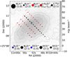 |
Fig. 1 Multi-pointing grids overlaid with the SCUBA-2850 µm map. The black dots in a (∆RA, ∆Dec)=(10″, 10″)-spacing 45º-cut show the pointings of IRAM 30-m and GBT observations. The red dotted grid shows the pointings of JCMT observations. The circles at the top and bottom indicate the beam sizes (θMB) of each spectral observation with the same color as the pointing grid except that GBT beam sizes are shown in blue. The 850 µm map is shown in grayscale with a beam size of 14″ and overlaid with its contours at 0%, 20%, 40%, 60%, and 80% of its peak intensity at 78 mJy beam−1. |
2.1.1 IRAM, JCMT, and GBT observations
We observed L 1498 in N2H+ (1–0), N2H+ (3–2), N2D+ (2– 1), DCO+ (2–1), DCO+ (3–2), and C18O (2–1) using the IRAM 30-m telescope in December 2013, May and October 2014, and September 2017. The observations were performed in frequency-switching mode using the dual polarization Eight MIxer Receiver (EMIR), the VErsatile SPectral Autocorrela-tor (VESPA), and the Fourier Transform Spectrometer (FTS). The spectra were observed on a (∆RA, ∆Dec)=(10″, 10″)J2000-spacing grid in a northeast-southwest cut across the core center at (RA, Dec)J2000 = (4h10m52s.97, +25° 10′ 18.″0). The data were subsequently folded and baseline subtracted with CLASS1. In addition, we complemented our observations with the data of N2H+ (1–0) and C18O (1–0) obtained by Tafalla et al. (2004). We refer readers to the observational details described by Tafalla et al. (2004). Their observation was conducted on a (ARA, ADec)B1950=(20″, 20″)-spacing grid. The spectral intensities, expressed in the TMB scaie, are consistent between our N2H+ (1–0) observations and theirs after adopting the historical main beam efficiency (ηMB) of 0.78 (Greve et al. 1998) for their observations and the current ηMB of 0.85 for our new observations. We also produce the N2H+ (1–0) integrated intensity map with CLASS (see Fig. 2i).
We performed the H2D+ (110–111) and N2H+ (4–3) observations in December 2015 using the 16-pixel HARP receiver equipped on JCMT (Buckle et al. 2009), which had two non-functioning pixels, in frequency-switching mode. The HARP array was rotated by 45° during the observation. In the JCMT-pointing grid shown in Fig. 1, the spacing is 15″ along the northeast-southwest direction and 30″ along the northwest-southeast direction. Data are converted to the CLASS format to be reduced with CLASS (folding and baseline subtraction).
The N2D+ (1–0) and DCO+ (1–0) observations were carried out in November 2014 using GBT. We used the MM1 and MM2 W-band dual polarization sub-band receivers in in-band frequency-switching mode with the Versatile GBT Astronomical Spectrometer (VEGAS) backend. The spectra were observed on the same northeast-southwest cut as the IRAM 30-m observations. Data were preprocessed in the GBTIDL data reduction program and converted to the CLASS format for subsequent reduction. The data were reduced by applying a technique where no OFF observation is subtracted (total power mode) to gain  in sensitivity. This technique utilizes two displaced spectra (ON and OFF observations) obtained in the frequency-switching mode by realigning and averaging these spectra, instead of subtracting and folding them in the standard reduction procedure, as explained in Pagani et al. (2020). The above spectral observations were conducted together with the previous L 1512 observations (Lin et al. 2020). We refer readers to the observational details described by Lin et al. (2020).
2.1.2 Calibration
Our spectral data are presented in the  scale throughout this paper instead of the TMB scale (see Fig. B.1). For extended sources like L1498, the TMB scale can introduce an overcorrection for low main-beam efficiencies (ηMB) (Bensch et al. 2001), particularly in the 1.3–0.8 mm range observed with the IRAM 30-m telescope and also in the 4 mm range observed with the GBT (see Table 1). In such cases, the error beams can pick up a substantial fraction of the signal of extended sources. Therefore, we directly analyze our data in the
  scale in Sect. 4.2 by considering the telescope beam response coupling to L 1498 based on the main beam and error beam efficiencies of the IRAM-30m telescope (see the online table2) and GBT (see Appendix A). For the archival IRAM-30m N2H+ (1–0) and C18O (1-0) data obtained by Tafalla et al. (2004) (see Fig. C.1 and the bottom row in Fig. D.1), we adopted the historical main and error beam efficiencies measured by Greve et al. (1998). On the other hand, we consider only the main beam response coupling for our JCMT H2D+ (110–111) and N2H+ (4–3) submillimeter observations due to the unavailability of error beam measurements for JCMT, as noted by Buckle et al. (2009). Despite this limitation, we find that the H2D+ emission area is less extended (see the H2D+ spectra in Figs. B.1 and C.2), whereas the N2H+ (4–3) line is not detected. Hence, there is a less pronounced contribution from extended structures that the error beams would pick up.
2.2 Continuum observations
2.2.1 JCMT observations
The Submillimeter Common-User Bolometer Array 2 (SCUBA-2; Holland et al. 2013) 850 µm observations of L 1498 were performed in August 2021 and August 2022. Four observations were taken in Band 2 weather (0.05 < τ225 GHZ < 0.08) under project codes M21BP043 and M22BP041 (PI: Sheng-Jun Lin), as supplementary SCUBA-2 projects of the ongoing JCMT BISTRO-3 (B-fields In STar-forming Region Observations 3) survey (PI: Derek Ward-Thompson). The analysis of the SCUBA-2 photometric data combined with the polarimetric data from the BISTRO-3 survey will be presented in a forthcoming paper as part of the BISTRO-3 series.
Each SCUBA-2 observation consists of 44 min of integration with the PONG-900 scan pattern, which fully samples a 15′ diameter circular region. The telescope beam size is 14″ at 850 µm. To account for the typically faint and extended nature of starless cores, we processed the raw data using the skyloop routine, employing a configuration file optimized specifically for extended emissions3, provided by the SMURF package in the Starlink software suite (Chapin et al. 2013). Figures 1 and 2h show the reduced data. The map was gridded to 4″ pixels and calibrated using a flux conversion factor (FCF) of 495 Jy pW−1 (Mairs et al. 2021). The average rms noise in the central 15′ field of the map on 4″ pixels is found to be ~4 mJy beam−1.
2.2.2 Canada-France-Hawaii Telescope (CFHT) and Spitzer observations
The CFHT Wide InfraRed CAMera (WIRCAM) was used with the wide filters J, H, and Ks to observe the source on the night of 26 December 2013. Seeing conditions were typically 0.″8, and the on-source integration times were typically 0.5–1 h per filter, to reach a completion magnitude of 21.5 (J band) to 20 (Ks band). We refer readers to the reduction details described by Lin et al. (2020). Spitzer observations are collected from the Spitzer Heritage Archive (SHA)4. L 1498 was observed with Spitzer InfraRed Array Camera (IRAC) in two programs: Program id. 94 (PI: Charles Lawrence) and Program id. 90109 (PI: Roberta Paladini); the second program occurred during the warm period of the mission (only 3.6 and 4.5 µm channels still working). The data taken from Program id. 94 were already discussed in Stutz et al. (2009), while the data taken from Program id. 90109 are analyzed in Steinacker et al. (2015). These two papers give the observational details. During the warm mission, deep observations of the cloud were performed and a completion magnitude of 18.5 in band IRAC2 (4.5 µm) was reached.
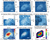 |
Fig. 2 L 1498 maps of continuum, extinction, and line integrated intensity. The CFHT NIR maps at the (a) J band, (b) H band, and (c) Ks band. Spitzer MIR maps at (d) IRAC1 band, (e) IRAC2 band, and (f) IRAC4 band with its contours at 7.0 MJy sr−1. (g) Visual extinction map with a beam size of 50″ with contours at 2.5, 5, 10, 15, 20, 25 mag. (h) JCMT SCUBA-2 850 µm map with a beam size of 14″ and the contours shown in Fig. 1. (i) Integrated intensity maps of N2H+ J=1–0 from Tafalla et al. (2004), calculated within VLSR=[−0.5 km s−1, 15.2 km s−1] with its contours at 20, 40, 60, 80% of its peak at 2.5 K km s−1 and a beam size of 26″. The central cross in each panel indicates the center of L 1498. The scale bars of 0.05 pc and AV/millimeter-wavelength beam sizes are denoted in the bottom right and bottom left corners, respectively. |
3 Results
3.1 Continuum maps
The continuum maps of L 1498 at near-infrared (NIR), mid-infrared (MIR), and submillimeter wavelengths are shown in Fig. 2. With the benefit of the deep NIR and MIR observations, the cloudshine phenomenon (Foster & Goodman 2006) is detected at J, H, and Ks bands, while the coreshine phenomenon (Pagani et al. 2010; Steinacker et al. 2010; Lefèvre et al. 2014) is detected at IRAC1 and IRAC2 bands. This cloudshine and coreshine detection indicates the presence of dust grain growth (Steinacker et al. 2015). We analyze the dust extinction in the above deep J, H, Ks, and IRAC2 images to derive the visual extinction map with a beam size of 50″ shown in Fig. 2g. We attempt to derive the total column density all over the cloud using the AV map with the benefit that the dust extinction is dependent on the dust density but independent of the dust temperature (Pagani et al. 2004, 2015; Lefèvre et al. 2016). However, because of the high extinction toward the core center, the lack of sufficient Ks-band stars prevents us from deriving the actual AV peak value, and instead we obtained a lower limit of AV at 25 mag toward the core center. This AV map is provided as a constraint on the outer density profile derived by the N2H+ line emission (see Sect. 4.4).
The 850 µm dust continuum emission observed by JCMT (Fig. 2h) is optically thin and sensitive to the cold dust in the core. With a much smaller 850 µm beam size of 14″ compared to that of the AV map, it clearly reveals the northwest-southeast-elongated core shape with a concave edge at the southern side.
Compared with the N2H+ (1-0) integrated line intensity map (Fig. 2i) with a beam size of 26 obtained from Tafalla et al. (2004), we can see that both the 850 µm continuum emission and the N2H+ (1–0) emission peak at the same position and have similar emission distributions, which implies that both trace the same region. Therefore, we use the 850 µm continuum map and the N2H+ (1–0) integrated intensity map to determine the core center of L 1498 to be (RA, Dec)J2000 = (4h10m52.97, +25° 10′ 18.″0). We can see that the chosen core center also coincides with the absorption center on the IRAC4 image (Fig. 2f), where the absorption feature is associated with the inner region of the core (Lefèvre et al. 2016). We denote the core center as a cross shown in each panel of Fig. 2.
3.2 Molecular emission lines
Figure 1 shows the pointings of our observations. Our IRAM 30-m and GBT pointing observations are performed along a northeast-southwest cut across the core center, and one row in the JCMT pointings is overlaid on the same northeast-southwest cut. We used this cut (hereafter, the main cut) to analyze the physical and chemical properties of L 1498 (Sect. 4). FigureB.1 shows the spectra of each emission line in the <ieq/ >scale along the main cut.
The L 1498 core is quiescent. Each hyperfine component of N2H+ (1–0) and N2D+ (1–0) is well separated. Along the main cut, the coverage of the N2H+ (1–0), N2H+ (3–2), DCO+ (1–0), and DCO+ (2–1) spectra span across the whole core. Including the N2D+ and o-H2D+ observations, we can see that the spectral intensities of these four cations peak toward the central region, suggesting that these cations are tracers for the core region. Meanwhile, N2H+ (4–3) shows no detection beyond the 3σ significance because of the low temperature inside the core and low central density compared to the critical density for this line (~ 2 × 107 cm−3 at 10 K). On the other hand, the o-H2D+ (110–111) line is detected in a smaller elongated region with an extent of ~30″ along the main cut and ~60″ perpendicular to the main cut (also see Fig. C.2). This indicates that o-H2D+ traces the innermost region of the L 1498 core. We note that this is the first o-H2D+ (110–111) detection toward L 1498. Caselli et al. (2008) conducted a survey of o-H2D+ (110–111) in nearby dense cores with the CSO 10.4-m antenna. However, L 1498 is one of the two undetected targets out of ten starless cores in their sample, indicating that the deuterium fractionation in L 1498 is relatively low compared with the other starless cores of their study. Their nondetection is probably because their rms noise of ~ 130 mK in the TMB scale is larger than our rms noise of ~50– 85 mK in the same scale (see Table 1). In addition, we also have a few C18O (2–1) spectra observed along the main cut, and their intensity shows a clear decrease in the central region, although the minimum spectral intensity does not occur at the core center but at (−20″, −20″).
4 Analysis
4.1 Objective and modeling strategy
We aim to provide a 3D physical description of L 1498 and estimate the chemical timescale of the deuteration fractiona-tion. To accomplish this goal, we utilized non-LTE radiative transfer modeling to analyze molecular line emissions, enabling us to evaluate the physical structure and molecular abundance profiles of the core. This abundance analysis is essential for estimating the chemical timescales of observed X(N2D+)/X(N2H+ ) ratios and other deuterated molecular abundances through time-dependent chemical modeling.
In the non-LTE radiative transfer modeling, we approximated the physical structure of L 1498 as two half onion-like models stuck together, comprised of multiple concentric homogeneous layers. The parameters in each layer are number density ( ), gas kinetic temperature (Tkin), relative abundances with respect to H2 of the observed species (
 ), turbulent velocity (Vturb5), rotational velocity field (Vrot), and radial velocity field (Vrad). The layer width is chosen to be
  arcsec (≈ 14.1″ and 1980 au at the distance of 140 pc), the same as the diagonal spacing of our IRAM 30-m/GBT pointing observations along the main cut. We therefore can determine these parameters at each layer sequentially from the outermost to the innermost layer by sampling sightlines of progressively decreasing radius along the main cut across L 1498.
Despite observations indicating an infall motion within the L 1498 envelope (Lee et al. 2001; Lee & Myers 2011; Magalhães et al. 2018), the L 1498 core remains quiescent, as evidenced by the single-peaked spectra observed in our study. Furthermore, the velocity gradient of N2H+ within this region is characterized by small magnitudes and seemingly random orientations, with a reported mean magnitude of 0.5±0.1 km s−1 pc−1 and a direction of 9°±10° (Caselli et al. 2002). Based on these observations, we have proceeded with the assumption that Vrad = 0 and Vrot = 0.
Then our procedure to determine these parameters at each layer is as follows. First, we used multi-transition N2H+ spectra to determine the  , Tkin, and X(N2H+) profiles, assuming a uniform Vturb value. Second, we determined the abundance profiles of N2D+, DCO+, and o-H2D+ by assuming that they share the same density, temperature, and kinematic properties of N2H+. The details of the radiative transfer modeling are explained in Sect. 4.2. With the obtained abundance profiles of N2H+, N2D+, DCO+, and o-H2D+, we employed a pseudo-time-dependent chemical model (Pagani et al. 2009b) to estimate the chemical timescales of each layer with our derived density and temperature profiles. In this adopted chemical model, the free parameters include the abundances of CO and N2, the initial OPR of H2 (OPRintial(H2)), the average grain radius (agr), and the cosmic ray ionization rate (ξ). These parameters are either determined or assumed with chosen values during the modeling process. Further details of the chemical modeling are explained in Sect. 4.3.
We basically followed the procedure in Lin et al. (2020), with the main difference being the construction of an asymmetric onion-like model for L 1498. Additionally, while Lin et al. (2020) independently determined  using the NIR/MIR dust extinction measurements, we simultaneously determined
  along with Tkin, X(N2H+), and Vturb by reproducing our multi-transition N2H+ spectra through radiative transfer modeling. This was due to the lack of sufficient Ks-band stars, which prevented us from deriving the actual AV peak value but allowed us to establish a lower limit of AV toward the core center (see Sect. 4.4). Thus our dust extinction map served primarily as a constraint on the
  profile at outer radii, where AV can be determined. We will further discuss the agreement of the dust extinction with our <ieq/ >in Sect. 5.1.
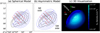 |
Fig. 3 Onion-like physical models. (a) The spherical model with the layer width as |

4.2 Radiative transfer applied to the onion-like physical model
Figures 3a and b show two onion-like models of L 1498. One is 1D spherically dissymmetric and the other is 3D asymmetric (see Appendix E). With our spectral observations along the main cut, we assumed that both models comprise nine and five layers on the southwest and northeast sides, respectively. In order to reproduce our observed spectra, we adopted a 1D spherically symmetric non-LTE radiative transfer code (MC; Bernes 1979; Pagani et al. 2007) for the 1D spherical case, and the Simulation Package for Astronomical Radiative Transfer/Xfer code (SPARX6) for the 3D asymmetric case. In both codes, we turned on the hyperfine-line-overlapping feature, and provided the updated hyperfine-line-resolved collisional rate coefficients (Lique et al. 2015; Pagani et al. 2012; Lin et al. 2020). We then obtained our modeled spectra calibrated in the scale, whereas the TMB scale can introduce an overcorrection for low main-beam efficiencies, ηMB (Bensch et al. 2001). Particularly in the 1.3–0.8 mm range observed with the IRAM 30-m telescope and also in the 4 mm range observed with the GBT, the error beams can pick up a substantial fraction of the signal of extended sources (see Sect. 2.1.2). This leads to overestimates of the temperature and/or density and also has an impact on the molecular abundance and the abundance ratio. Calibrating in the  scale by considering the telescope coupling contributions from the main beam and error beams allows for a better representation of extended sources without having to handle the corrections of the error beam pick-up in the TMB scale (see Appendix A).
We search for the best-fit profiles of  , Tkin, abundances of our observed species, and Vturb with the 1D spherical model by our spectral fitting procedure. Initially, we ran MC to reproduce our N2H+ (1–0, 3–2, and 4–3) spectra across the main cut. This allowed us to determine
  , Tkin, X(N2H+), and Vtrub layer by layer, sequentially from the outermost to the innermost layer, for both the northeast and southwest sides. We found that a uniform Vturb of 0.09 km s−1 can reproduce the spectral line widths along the main cut, with all spectra consistent with a systematic velocity of 7.8 km s−1. These initial
  , Tkin, and X(N2H+ ) profiles served as the initial guess for refinement. Subsequently, we used the simulated annealing (SA) algorithm provided by the Modeling and Analysis Generic Interface for eXternal numerical codes (MAGIX; Möller et al. 2013) to optimize the fit of the N2H+ spectra, obtaining the best-fit profiles of
  , Tkin, and X(N2H+) from our initial profiles. The 1σ uncertainty of each parameter at every layer was determined using the interval nested sampling error estimation method provided by MAGIX, with the other parameters fixed. Afterward, we determined the abundance profiles of N2D+, DCO+, and o-H2D+, along with their respective 1σ uncertainties, by fitting the spectra of N2D+ (1–0, and 2–1), DCO+ (1–0, 2–1, and 3–2), and o-H2D+ (110–111). This fitting process assumed identical
  and Tkin profiles, as well as a constant Vturb, as for N2H+. Because of our shorter spatial coverage in the N2D+ observation, we limit X(N2D+) in the outer layers with X(N2D+)/X(N2H+) lower than the observed minimum X(N2D+)/X(N2H+) of 0.07. The best-fit central
  was found to be
  , and the central
  .
.
Next, we transform the above best-fit profiles from the 1D spherical model to the 3D asymmetric model because carrying out a non-LTE calculation with a 3D asymmetric model repeatedly in the fitting is much more numerically expensive than the 1D case. Our 3D asymmetric model was designed to follow the emission morphologies of the 850 µm continuum and the N2H+ (1–0) integrated intensity. We set the southwest sides in both models to have identical physical parameters and abundance profiles. For the northeast side, the spherical model was stretched along the sightline direction by a factor of ~2 to match the thickness of the southwest side along the line of sight (see AppendixE). Keeping the same northeast profiles in the asymmetric model results in too strong intensities in the spectra because the molecular abundances are doubled. We aim to keep the continuity in the  and Tkin profiles across two sides, so we simply divided the abundances in the northeast sides by a common factor of ~2 to make the modeled spectra fit with the observations. We note that our intention is to obtain a simultaneous fit that is generally consistent with the observational spectra since performing a complete search of the entire parameter space for the best possible fit is not achievable.
Figure 4 shows our best-fit profiles of  , Tkin, abundances of the above four cations, and the N2H+ deuteration ratio, X(N2D+)/X(N2H+), along the main cut across the center of our asymmetric onion-like model, while Fig. 3c shows the 3D visualization of the
  distribution. We also fit our
  profiles with the Plummer-like profile with
  , where n0, R0, and η are central density, flattening radius, and the power-law index, respectively. The fitted Plummer-like profiles are shown with green curves and the fitted parameters are annotated (n0 = 1.6 × 105 cm−3, R0 = 8.2 kau and η = 2.23 for the southwest profile, and R0 = 3.0 kau and η = 2.30 for the northeast profile) in the top row in Fig. 4. The above best-fit profiles are also numerically listed in Table F.1. In addition, in Fig. 4, the
  , Tkin, and X(N2H+) profiles of the spherical model found by Tafalla et al. (2004) are also shown in purple. Since their model center was chosen at a different position with an offset of (∆RA = −10″, ∆Dec = −20″) with respect to our model center, we compute these purple curves along our main cut (i.e., a secant line of their spherical model) using their parameters (see their Tables 1 and 3). We will further discuss the discrepancy between our and their models in Sect. 5. Finally, the best-fit modeled spectra of the four cations along the main cut are shown in red in Fig. B.1. In addition, Fig. C.1 shows our best-fit modeled N2H+ (1–0) spectra overlaid on the data from Tafalla et al. (2004), while Fig. C.2 shows our best-fit modeled o-H2D+ (110– 111) spectra overlaid on our full o-H2D+ data. Our reproduced spectra are in good agreement with the observations, suggesting that our model is globally valid for the L 1498 core.
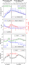 |
Fig. 4 Physical and abundance profiles along the main cut. The profiles of number density ( |


4.3 Time-dependent chemical model
We estimated the chemical timescale of each layer in the onion model of L 1498 with our derived abundance,  and Tkin profiles. Our method adopted a pseudo-time-dependent gas-phase deuterium chemical model (Pagani et al. 2009b) to simultaneously reproduce the deuteration ratio, X(N2D+)/X(N2H+), and the abundances of N2H+, N2D+, DCO+, and o-H2D+ in each layer. This deuterium chemical model is specialized for starless cores in that each spin state of the H2 and
  isotopologues are included and the complete depletion in heavy species, except for CO and N2, is assumed. In our model, we did not include the nitrogen chemistry. CO and N2 would quasi-instantaneously reach chemical equilibrium with our observed species because our chemical network is very small. On one hand, CO and N2 are the parent molecules reacting with the
  isotopologues to form the N2H+ and HCO+ isotopologues (i.e., the daughter cations); on the other hand, dissociative recombination of these daughter cations would convert them back to CO and N2 . The abundances of CO and N2 are left as free parameters in each layer, so we could derive the current CO and N2 abundance profiles. The other free parameters are the initial OPR of H2 (OPRintial(H2)), the average grain radius (agr), and the cosmic ray ionization rate (ξ).
Figure 5 shows the best-fit chemical model solutions of X(N2D+)/X(N2H+), X(o-H2D+), and X(DCO+) for each layer at the northeast and southwest sides. The outermost layers were not modeled simply because their large observational error bars cannot well-constrain the chemical solutions. For these chemical solutions, the initial OPR of H2 is assumed to be its statistical ratio of 3. We adopted the ξ of 3 × 10⁻¹⁷ s−1 throughout the chemical model, which is the best value found by Maret et al. (2013) for their chemical model to reproduce the C18O (1–0) and H13CO+ (1–0) integrated emission in L 1498. With the detection of coreshine, one would expect that larger dust grains (agr > 0.1 µm) appear in the core (Pagani et al. 2010; Steinacker et al. 2010; Lefèvre et al. 2014). Although Steinacker et al. (2015) cannot well constrain the maximum grain radius in L 1498 with the coreshine modeling on the IRAC1/2 images, they suggested that the maximum grain radius seems to be greater than ~0.3 µm. On the other hand, Maret et al. (2013) found that in their chemical model, a power-law grain size distribution grown from the typical grain radius of 0.1 µm to a maximum grain radius of 0.15 µm is sufficient for reproducing the C18O and H13CO+ line emissions, suggesting that the grain growth does not yet significantly occur everywhere in the entire core. The apparent contradiction of the maximum grain radius reported by Maret et al. (2013) and that reported by Steinacker et al. (2015) arises because the low-J transitions of C18O and H13CO+ are optically thick, and as such, they do not trace the core center but rather the low-density outskirts. Thus, these indicate that agr ≳ 0.3 µm at the center of L 1498 while agr ≈ 0.1 µm at the outskirts. The bottom row in Fig. 6 shows the profiles of the grain radius in our chemical model. In order to make the chemical solutions match the observational abundances, we found that the grain radius should be at least 0.4 µm in the innermost layer, and 0.2 µm in the second layer. For the rest of the layers, we found matched chemical solutions with the typical grain radius of 0.1 µm. With the above conditions, we found that the observational abundances of all layers are matched with chemical solutions from 0.07 to 0.31 Ma on the northeast side, and from 0.08 to 0.31 Ma on the southwest side.
The top row in Fig. 6 shows the CO and N2 abundance profiles from our chemical modeling. Their best-fit values are listed in Table F.1. Error bars show the abundance ranges of the possible chemical solutions at each layer but not every combination of X(CO) and X(N2) can make the chemical solutions fit the observational cation abundances. We assume a constant 12C16O/12C18O ratio of 560, which is comparable to the local 16O/18O ISM ratio of 557±30 (Wilson & Rood 1994), to derive a C18O abundance profile. The C18O line emission from the central depleted region is too weak to be constrained by radiative transfer calculation. Our chemical model serves as an appropriate approach. At the outer layers, X(CO) is less constrained since deuteration is only an upper limit in the chemical models. By contrast, C18O is not heavily depleted and its J=2– 1 line emission remains thinner and thus the radiative transfer modeling is applicable. We then used our C18O (2–1) observation to further determine the outer CO abundance (southwestern layer 4–8, and northeastern layer 2–4). With radiative transfer calculations, we found an outer X(C18O) of 1.9 × 10⁻⁸ can roughly make the C18O (2–1) spectrum models fit with observations (the last row in Fig. B.1), validating our chemical modeling results. We then set the outer X(12CO) as 1.0 × 10⁻⁵.
We noted that the C18O (2–1) spectra around the pointing from (−10″, −10″) to (−40″, −40″) are somewhat lower in intensities compared to our modeled C18O spectra. It seems to be caused by a more considerable depletion along the line of sight toward these positions. It is possible that the C18O depletion center shifted outward from the core center that we determined by the emission peak position shared by 850 µm continuum, N2H+ and o-H2D+ data (also see the C18O J=1–0 and 2–1 integrated intensity maps shown in Fig. 3 from Tafalla et al. 2004). This would hint that the CO isotopologues have a more complex spatial cloud structure along the line of sight.
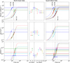 |
Fig. 5 Chemical modeling of the abundance ratio of N2D+/N2H+ and the abundances of o-H2D+ and DCO+ for each layer. Left and right columns: chemical model solutions (curves) and the observationally derived values (horizontal lines). Middle column: observationally derived profiles with uncertainties from Fig. 4. The model solutions and observed values are color-coded by different layers. The models are calculated with an initial OPR(H2) of 3, a cosmic ray ionization rate (ξ) of 3 × 10⁻¹⁷ s−1, and an average grain radius (agr) profile shown in Fig. 6. The two dashed-dotted vertical lines in each panel indicate a time range for which the model values cross the observations within their error bars, and we make such model curves thicker. The thick model curve is displayed as dashed if the observation only has an upper limit. The solid vertical line indicates the lower limit on the core age of L 1498 as 0.16 Ma. |
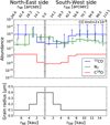 |
Fig. 6 Profiles of the abundances CO, N2, and the grain radius (agr). The X(12CO), X(N2), and agr profiles are the best-fit results from the chemical modeling. The X(C18O) profile is obtained by assuming a 12CO/C18O abundance ratio of 560 or a constant value of 1.9 × 10⁻⁸. |
4.4 Visual extinction
Similar to the procedure in Lin et al. (2020), we used the NIR/MIR images (Fig. 2) to derive the visual extinction map with the NICER method (Lombardi & Alves 2001). We used the J, H, and Ks images with the RV = 3.1 dust models from Weingartner & Draine (2001) to make an envelope extinction map tracing the L 1498 envelope. On the other hand, we used the H, Ks, and IRAC2 images with the RV = 5.5B dust models from Weingartner & Draine (2001) to make a core extinction map tracing the L 1498 core. However, the lack of sufficient stars with the color excess  measurements prevents us from deriving the extinction at the core center. Although many stars appear on the IRAC1/2 images, only a few stars are detected in the Ks band in the core region, and we found that the magnitude differences of the Ks and IRAC2 bands (
 ) for these stars approach 2.5 mag toward the center. This magnitude difference is already larger than the difference between the completion magnitudes of Ks and IRAC2 bands (20 and 18.5 mag, respectively), which explains the disappearance of the Ks-band counterparts. Therefore, we assume that the Ks-band magnitude of stars only detected in IRAC2 bands have
  mag, and we generated the artificial Ks-band detection by
selecting stars that are (a) detected in both IRAC1 and IRAC2 bands to ensure it is not due to contamination in a single band and (b) with the IRAC2 magnitude uncertainty less than 0.2 mag, and
assigning their Ks-band magnitude as mIRAC2 + 2.5 mag, that is, the brightest limit from the above assumption, resulting in a lower limit of
 and AV.
After this process, the density of stars with color excess measurements across L 1498 allowed us to convolve the reddening data with a 50″-Gaussian beam to produce the core and envelope extinction maps. We combined the core map and envelope map by merging them at 5 mag and the final AV map has been shown in Fig. 2g and the insert of Fig. 7. Stars only detected in the IRAC1/2 bands and with the artificial Ks-band detection are displayed as black dots on the insert of Fig. 7. Figure 7 also shows the radially averaged AV profiles along the main cut within the 50''-wide strip. As a result, the AV values in the central region should be interpreted as the lower limit, and therefore our result suggests that AV ≳ 25 mag at the 50″-beam.
5 Discussion
As shown in Sect. 4, we built an asymmetric onion-shell model of L 1498 to evaluate its physical structure and chemical abundances shown in Figs. 4 and 6. Our model can well reproduce the observed spectra along the main cut shown in Fig. B.1 via the non-LTE radiative transfer calculations. In this section, we compare our findings with other studies and address the core age of L 1498.
5.1 Density and kinetic temperature
With our non-LTE radiative transfer modeling on the N2H+ emission line spectra, we find a central  of
of  and
and  , and a peak
  toward the L 1498 core. With the submillimeter data, Tafalla et al. (2004) derived
  with Td = 10 K using the IRAM 30-m MAMBO 1.2 mm map. In contrast, our
  peak value is slightly larger than that of Tafalla et al. (2004) This discrepancy could be due to our different approach using the radiative transfer modeling of the line emission instead of the continuum emission. The crucial uncertainty in the non-LTE line modeling is the collisional coefficients, which is, however, much smaller than the uncertainty in the dust opacity at the submillimeter wavelength. On the other hand, Tafalla et al. (2004) adopted a uniform Tkin of 10 K derived from NH3 (1,1) and (2,2) lines as Td by assuming the gas and dust are coupled. However, the lower critical density of these NH3 lines (~2 × 103 cm−3; Pagani et al. 2007) compared to the N2H+ J=1– 0 line (1.3 × 105 cm−3 at 10 K) would suggest that N2H+ can trace the inner Tkin better than NH3. Therefore, using 10 K may underestimate the density at the core center.
Another distinction is that our onion model is asymmetric, while Tafalla et al. (2004)’s model is spherically symmetric. The top row in Fig. 3 shows the comparison between our number density profiles and those of Tafalla et al. (2004). We can see that our  profiles and theirs converge toward the outer southwestern region. While the spherical onion model adopted by Tafalla et al. (2004) provides a good approximation for deriving an averaged density profile of the elongated L 1498 core, Their model center (∆RA = −10″, ADec = −20″ with respect to ours) was based on the centroid of their 1.2 mm emission map rather than the emission peak. In contrast, our model center is situated at the JCMT SCUBA-2 850 µm continuum, N2H+ (1−0), and o-H2D+ (110− 111) emission peaks, including their 1.2 mm continuum peak. In this case, our chosen model center would allow us to capture the peak
  rather than average it out with the surrounding region.
Meanwhile, our NIR and MIR dust extinction measurements provide another constraint on the density in L 1498. Different from the dust emission measurement, the dust extinction is independent of Td, and the NIR/MIR dust opacity is better determined than the submillimeter dust opacity (Pagani et al. 2015; Lefèvre et al. 2016). Figure 7 shows the comparison of the AV profiles derived with the observational data and our onion model along the main cut. The orange and red squares represent the extinction at the 50″-beam of the whole L 1498 cloud (i.e., the core and envelope) derived from NIR/MIR images and the central AV value is estimated as the lower limit (AV ≳ 25 mag; see Sect. 4.4). The gray and blue step curves represent the AV values contributed by the L 1498 core, which are converted from our asymmetric onion-like model by  cm−2 mag−1 (RV = 3.1; Bohlin et al. 1978), and the blue curve is convolved with the AV beam size of 50″ for the comparison with the data. Our onion model represents the core region because it was constructed from the N2H+ data, a molecule confined in the core region. We can see that the AV profile of our onion model matches well with the data in the core region. The AV profile of the data consists of the extinction from the L 1498 core and from an envelope with AV ≈ 3 mag. Since our observations of N2H+, N2D+, DCO+, and o-H2D+ are associated with the core as these molecules are mostly confined in the core region, we do not need to include the envelope to reproduce their observational spectra shown in Fig. B.1. In Appendix D, we show that including an envelope with AV = 3 mag in the radiative transfer model can still reproduce our C18O (2−1) spectra (the bottom row in Fig. B.1), whereas it is necessary for reproducing the C18O (1− 0) spectra obtained by Tafalla et al. (2004) with a lower critical density.
With the interferometer, the ALMA-ACA 1 mm continuum survey, FREJA (Tokuda et al. 2020), found no substructure at the 1 kau scale in the central region of L 1498, suggesting that the central density structure is very flat (characterized by a Plummer-like flattening diameter greater than 5 kau) and an upper limit on  of about 3 × 105 cm−3. This nondetection is in agreement with the
  profile evaluated from our onion model with the central density of
  and the central flattened region size of ~ 11 kau (R0,SW + R0,NE; see the Plummer-like parameters shown on the top row in Fig. 3). Therefore, our solution from the non-LTE N2H+ radiative transfer modeling is compatible with the NIR/MIR dust extinction measurement as well as the 1mm continuum interferometry observation.
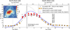 |
Fig. 7 Comparison of the NICER-derived AV profile and the AV profile derived from the column density from the best-fit asymmetric onion-like model along the main cut. The black crosses are the NICER-derived AV values at each pixel in the 50″-wide strip on the AV map shown as the insert. The orange and red squares with error bars show the radially averaged AV profile with the 14.1″-bin from the strip, where the central region is represented as lower limits due to the lack of the Ks-band detections. The gray step curve shows the AV profiles converted from our onion-like model, while the blue step curve is convolved with the AV-beam of 50″. The coverage of our onion-like model is shown by black dashed lines. The insert shows the NICER-derived AV map with the 50″-beam (Fig. 2g) overlaid with black dots, indicating the stars only detected in the IRAC1/2 bands but with the artificial Ks-band detection (see Sect. 4.4). |
5.2 Cation abundance profiles
We find that N2H+ is significantly depleted toward the L 1498 center with a depletion factor of  with respect to the maximum X(N2H+) at the fifth southwestern layer, and another depletion factor of
  with respect to the maximum at the second northeastern layer (see Fig. 4). Since the northeastern depletion feature is only resolved by two layers in the onion model, we take the depletion factor measured on the southwest side as the representative measurement in the following discussion (same for the other molecules). Our finding of the N2H+ depletion is opposite to the N2H+ enhancement by a factor of 3 reported by Tafalla et al. (2004) with their radiative transfer modeling. Our central N2H+ abundance is 4.7 ± 1.7 × 10⁻¹¹, while their value is 1.7 × 10⁻¹⁰. This discrepancy could be due to their different physical model and the approximation made in their radiative transfer calculations. Tafalla et al. (2004) derived a central
  , a factor of 1.7 lower than our
  , and a constant Tkin(NH3) = 10 K, higher than our
  K (see their
  , Tkin, and N2H+ abundance profiles on Fig. 3). As previously mentioned, using the temperature derived from the NH3 lines could be biased by the warmer outer layers and thus one could overestimate the central temperature. In addition, they omitted line overlap from their radiative transfer calculation in their customized version of the MC code, and the hyperfine-structure-resolved collisional coefficients were just not yet available. As a result, the peak intensities of their bestfit N2H+ (1−0) spectra were too strong by ~60% compared to data, but even with our current MC code, adopting their physical model would still result in ~30% stronger intensities at the peaks. In terms of the line-of-sight-integrated measurements, our averaged X(N2H+) and N2H+ column density (
 ) toward the core center are 1.2 × 10⁻¹⁰ and 5.2 × 1012 cm−2, respectively. Our
  value is of the same order of magnitude compared with 1.7 ± 0.7 × 1012 cm−2 reported by Crapsi et al. (2005) despite their more simplistic LTE calculations.
Interestingly, both N2H+ depletion and enhancement are seen from chemo-dynamical modeling. Aikawa et al. (2005) performed a self-consistent calculation with a quasistatically contracting Bonner-Ebert sphere, and found that N2H+ is enhanced at a central  similar to L 1498 (1.5 × 105 cm−3) and later becomes depleted at higher densities. Holdship et al. (2017) and Priestley et al. (2018) used an analytical approach for the BonnerEbert density evolution, but found that the N2H+ depletion starts earlier in their calculation. Holdship et al. (2017) found an N2H+ depletion factor of ~50 when
  reaches Tafalla et al. (2004)’s best-fit value for L 1498. Although this discrepancy might relate to their N chemistry details in the models, the depletion case would be preferred by our findings.
In starless cores, the depletion of the N2H+ and HCO+ iso-topologues is a result of the freeze-out of their parent molecules (N2 and CO) in the core center. In L 1498, we find depletion factors of  for N2H+ and 17±11 for DCO+. However, in contrast, N2D+ does not exhibit significant depletion toward the core center (see Fig. 4). Here, we do not interpret the inward decrease in X(N2D+) on the northeastern side as significant depletion. This may be due to the limited coverage of our spectral observations in the northeastern area (see Fig. B.1). The lack of significant depletion in N2D+ is likely because the increase in deuteration of
  outweighs the decrease in N2 due to freeze-out. Regarding the deuteration of N2H+, we have observed a X(N2D+)/X(N2H+) profile spanning from an upper limit of 0.07 in the outer region to a maximum of
  toward the center of L 1498. However, this maximum value is moderate compared to values obtained in the other two starless cores, L 183 (Pagani et al. 2007) and L 1512 (Lin et al. 2020). The authors found a maximum N2H+ deuteration of 0.70±0.12 in L 183 and
  in L 1512. It is worth noting that the formation and destruction of N2D+ and DCO+ follow the same chemical scheme in starless cores (Pagani et al. 2011). Given that N2D+ and DCO+ are formed under the same conditions of
  deuteration, the presence of DCO+ depletion suggests that the depletion of CO is greater than that of N2.
5.3 CO and N2 abundance profiles
Molecular nitrogen is the parent molecule reacting with the  isotopologues to form N2H+ and N2D+, while CO is the parent molecule also reacting with
  isotopologues to form DCO+ (Pagani et al. 2011). In starless cores, N2H+, N2D+, DCO+ are formed via the above gas-phase paths. Therefore, as we presented in Sect. 4.3, X(N2) and X(CO) are free parameters for fitting the observed abundances of their daughter cations. The top row in Fig. 6 shows the abundance profiles of N2,12CO, and C18O. Both 12CO and C18O have the same depletion factors of ~20 compared with their maximum abundances of 1 0 × 10−5 for 12CO and 1.9 × 10⁻⁸ for C18O since we assumed a constant ratio of 12C16O/12C18O as 560 to derive the C18O profile from 12CO profile. By comparing with the standard 12CO abundance of (1−2) × 10−4 (Pineda et al. 2010), 12CO has a depletion factor of ~200−400. For C18O, the depletion factor is ~190 with respect to its standard abundance of 1.7 × 10⁻⁷ (Frerking et al. 1982). Conversely, the N2 abundance does not decrease but even increases toward the core center (Fig. 6). This accounts for the discrepancy between the depletion of DCO+ and the enhancement of N2D+ toward the core center.
In our chemical modeling, we find that the dust grain radius increases from 0.1 µm in the outer region to 0.4 µm in the core center. This grain growth slows down the depletion of CO and N2 due to freeze-out onto dust grains at the core center by a factor of ~3, as the depletion timescale is proportional to the dust grain radius (Maret et al. 2013). However, the freeze-out rates of CO and N2 are suggested to be similar because of their identical mass and similar binding energies (Bisschop et al. 2006). Also, the cosmic ray ionization is too weak in the dense core to compensate for the depletion of CO and N2. The discrepancy between the N2 and CO abundance profiles may suggest that the N2 production from the atomic N is still active such that the N2 production can compensate for the depletion of N2, similar to what Pagani et al. (2012) found in the core center of L 183. In contrast, the CO production has reached a steady state in the diffuse cloud region (Oppenheimer & Dalgarno 1975), making the freeze-out effect the dominant mechanism regulating the CO abundance in the dense core region.
With the envelope tracers of CO and HCO+, Maret et al. (2013) performed pseudo-time-dependent chemical modeling to study their depletion in L 1498. They constrained their model by fitting the integrated intensity profiles and the central spectra of C18O (1−0) and H13CO+ (1−0). To reproduce their observations, they found a maximum grain radius of 0.15 µm in the core center. Our maximum grain radius of 0.4 µm is greater than their value, likely because the four molecular cations (N2H+, N2D+, o-H2D+, and DCO+) we used are not heavily depleted and their emissions are optically thinner than the above envelope tracers. Therefore, our chemical modeling is more sensitive to the grain radius in the central region. Despite this difference, when they included such grain growth in their chemical modeling, they derived a central CO abundance of ~ 6 × 10⁻⁷, which is consistent with our value of  . In addition, their chemical network includes nitrogen chemistry. They found that a certain fraction of the nitrogen should be locked in NH3 ices to reduce the gasphase abundances of N2, and atomic N. As a result, they obtained aN2H+ abundance of 4 × 10⁻¹⁰, which is closer to the 1.7 × 10⁻¹⁰ value derived by Tafalla et al. (2004) (also see Sect. 5.2 for the comparison of our N2H+ abundance profile with Tafalla et al. 2004). However, our central X(N2H+) is even lower, at 4.7 ± 1.7 × 10⁻¹¹, and our central X(N2) at
  is larger than Maret et al. (2013)’s 2 × 10⁻⁷. Therefore, more detailed modeling is necessary to understand the nitrogen chemistry in L 1498.
5.4 Core age of L 1498
Figure 5 shows that between 0.07 to 0.31 Ma, the chemical solution of each layer appears at the observed abundances within the uncertainties. One important characteristic of deuterium chemistry in starless cores is that the deuteration fractionation can serve as an effective chemical clock. This is because it primarily depends on time and is influenced by a few initial parameters, including the initial ortho-to-para ratio of H2 (OPRintial(H2)), the cosmic ray ionization rate (ζ), and the average grain radius (agr). It is less affected by temperature and dynamical parameters such as the turbulent Mach number and the mass-to-magnetic flux ratio (Pagani et al. 2013; Kong et al. 2016; Körtgen et al. 2017). Therefore, given reasonable values/ranges of OPRintial(H2), ζ, and agr, the timescale of deuteration fractionation (i.e., the chemical timescale) provides a means to measure the age of a contracting core.
With pseudo-time-dependent chemical analysis, we have determined the chemical timescales of the deuteration in each layer in Sect. 4.3. Since the physical structure is kept constant at the present state in the pseudo-time-dependent models during the evolution of the chemical composition, our chemical timescales do not include the physical evolution of the core. Therefore, the determined chemical timescales at the fixed densities serve as a lower limit to the core age. Particularly, we take the chemical timescale of a less evolved outer layer, where X(N2D+)/X(N2H+) ratio and X(o-H2D+) are measured, to represent the lower limit of the core age. It follows that the lower limit on the core age of L 1498 is ~0.16 Ma determined by the fourth southwestern layer, which is the last layer with the N2D+/N2H+ ratio measurement, and this lower limit is conservatively chosen at the beginning of the time range of this layer. We would like to note that we use the X(N2D+)/X(N2H+) ratio and X(o-H2D+) to determine the chemical timescale of a layer, while we use X(DCO+) to derive the CO abundance. Since the fourth south-western layer has no o-H2D+ detection but only an upper limit on its abundance, the interpretation for this time limit is the time duration for reaching X(N2D+)/X(N2H+) under the assumption of X(o-H2D+) at the maximum of its possible range, that is, the fastest time of that layer.
Although deuteration fractionation depends on OPRintial(H2), ζ, and agr, we assumed OPRintial(H2) to be the statistical ratio of 3. Additionally, we adopted ζ = 3 × 10⁻¹⁷ s−1 from Maret et al. (2013) and the typical agr of 0.1 µm for the fourth southwestern layer (see Sect. 4.3). Therefore, L 1498 is presumably older than 0.16 Ma. If we assume another OPRintial(H2) of 0.5 as measured in the diffuse medium (Crabtree et al. 2011), we find another, but similar, age lower limit of 0.13 Ma. In the fast collapse model, the contraction timescale of the core can be characterized by the free-fall time, tff :
 (1)
(1)
where G is the gravitational constant and ρ represents the mass density, which can be expressed as  , where mH is the mass of atomic hydrogen and
  denotes the mean molecular weight per H2. Considering that dense starless cores are typically contracted from lower density gas at
  , tff = 0.31 Ma, which is compatible with the lower limit of the core age of L 1498 at 0.16 Ma. On the other hand, the core contraction timescale in the slow collapse model can be associated with the ambipolar diffusion timescale in the presence of the magnetic field support. The ambipolar diffusion timescale can be longer than a free-fall time by an order of magnitude (Shu et al. 1987; Tassis & Mouschovias 2004; Mouschovias et al. 2006; McKee & Ostriker 2007). Although a lower limit of the core age at 0.16 Ma does not conclusively rule out the possibility of a much longer actual core age, such a long contraction timescale does not seem to be favored by our findings. Particularly, significant inward motions have been detected toward the L 1498 envelope via CS lines (Lee et al. 2001; Lee & Myers 2011) and HCN lines (Magalhães et al. 2018). Therefore, our result suggests that the contraction of L 1498 follows the fast collapse model, indicating that L 1498 likely formed rapidly.
Maret et al. (2013) and Jiménez-Serra et al. (2021) also derived the chemical timescales of L 1498 but with different molecules. Maret et al. (2013) derived a chemical timescale of L 1498 with a range of 0.3-0.5 Ma based on the CO freeze-out modeling with the C18O (1−0) line, while Jiménez-Serra et al. (2021) derived a chemical timescale as 0.09 Ma from their COMs observation toward the methanol emission peak at the outer layers of L 1498. Because both studies employed the pseudo-time-dependent chemical analysis, their chemical timescales are also lower limits on the age of L 1498. It is noteworthy that although the timescale derived by Maret et al. is longer than our deuteration timescale, using their value as the lower limit of the core age would still favor the fast collapse model. In fact, X(CO) at the core center derived from our deuteration chemical modeling aligns with their derived CO value (see Sect. 5.3). However, assessing CO depletion toward highly embedded and more evolved cores can be challenging due to the contamination along the sightline and the severe CO depletion. In such cases, the deuteration fraction is easier to measure and can provide valuable insights into the chemical evolutionary history of the core contraction. Therefore, it is demonstrated that different chemical clocks provide a comprehensive point of view on the core ages. On the other hand, in the chemical modeling of COMs, the surrounding environment could be more important than chemical evolutionary effects (Lattanzi et al. 2020). Then COMs may not act as a chemical clock but as an indicator of the environmental conditions.
In this work, we discuss the low-mass core formation in the context of contrasting fast and slow collapse models of relatively isolated entities in the parent clouds. However, we note that the interactions between starless cores and their surrounding clumps and filaments may lead to more dynamical scenarios, such as fragmentation into smaller entities and mass accumulation or accretion from parent filamentary structures, suggesting a hierarchical nature (e.g., Vázquez-Semadeni et al. 2019). This complexity potentially aligns with scenarios favoring fast collapse. Recently, Bovino et al. (2021) performed a 3D turbulent MHD simulation coupled with deuterium chemistry to study a collapsing filament, fragmenting into dense cores. They proposed the o-H2D+ to p-D2H+ ratio as an alternative chemical clock to the N2D+/N2H+ ratio for tracing OPR(H2). Their APEX o-H2D+ (110−111) andp-D2H+ (110−101) observations of six starless cores in the Ophiuchus region demonstrate that fast collapse models align well with the observed o-H2D+/p-D2H+ ratios with core ages at ~0.05−0.2 Ma, indicating that these Ophiuchus cores can form more rapidly.
6 Conclusions
We present the first o-H2D+ (110−111) detection toward L 1498. We carried out a non-LTE radiative transfer calculation with an asymmetric onion-like model to reproduce the emission line of L 1498. We obtained 3D asymmetric profiles of the physical parameters and chemical abundances of N2H+, N2D+, DCO+, and o-H2D+. Then, we used a time-dependent chemical model adopting a deuterium chemical network to estimate the lower limit on the core age of L 1498 by fitting the chemical solutions to the observed abundances. We summarize our results as follows:
We derived the central molecular hydrogen density of
 and the central kinetic temperature of
  K from N2H+ observations, resulting in a peak
  of 4.5 × 1022 cm−2 toward the L 1498 core;
We found depletion factors of
 for N2H+ and 17±11 for DCO+. The deuterium fractionation of N2H+ is enhanced from an upper limit of ≤0.07 at large radii to
  in the center;
The opposite behaviors of the N2D+ enhancement and DCO+ depletion toward the core center suggest that the depletion of CO is greater than that of N2. Our results show that 12CO and C18O have a depletion factor of ~20 between internal and external layers in the core. Comparing their minimum abundance to their standard (literature) abundance, both isotopologues have comparable depletion factors of about 200;
We derived a lower limit on the core age of L 1498 as 0.16 Ma, which is comparable to the typical free-fall time of 0.31 Ma, assuming that starless cores contract from gas with a typical density of
 . Our result suggests that the contraction of L 1498 follows the fast collapse model, indicating that L 1498 likely formed rapidly.
In summary, our results show a self-consistent description of density, temperature, and molecular abundances in a starless core. We have expanded our investigation to include a survey of additional low-mass cores. Detailed modeling of our samples as well as comparison of them will shed light on discriminating factors in their evolution. We would offer a comprehensive understanding of core formation mechanisms by assessing their ages and dynamics.
Acknowledgements
The authors would like to warmly thank Mario Tafalla (Instituto Geografico Nacional Observatorio Astronómico Nacional, Spain) for providing his 1.2 mm MAMBO and molecular line maps, Sébastien Maret (Institut de Planétologie et d'Astrophysique de Grenoble, France) for providing his molecular line maps, Sheng-Yuan Liu and I-Ta Hsieh (ASIAA, Taiwan) for discussing the details of the SPARX code, David T. Frayer (GBT) for discussing the details of beam efficiencies, and Nawfel Bouflous and Patrick Hudelot (TERAPIX data center, IAP, Paris, France) for their help in preparing the CFHT/WIRCAM observation scenario and for performing the data reduction. S.J.L. acknowledges the grants from the National Science and Technology Council (NSTC) of Taiwan 111-2124-M-001-005, 112-2124-M-001-014, and 113-2124-M-001-008. S.J.L. and S.P.L. acknowledge the grants from NSTC of Taiwan 109-2112-M-007-010-MY3, 112-2112-M-007-011. This work used high-performance computing facilities operated by the Center for Informatics and Computation in Astronomy (CICA) at NTHU. This equipment was funded by the Ministry of Education of Taiwan, the Ministry of Science and Technology of Taiwan, and NTHU. This work was supported by the Programme National “Physique et Chimie du Milieu Interstellaire” (PCMI) of INSU/CNRS with INC/INP co-funded by CEA and CNES and by Action Fédératrice Astrochimie de l’Observatoire de Paris. This work is based in part on observations carried out under project numbers 152-13, 039-14, and 112-15 with the IRAM 30-m telescope. IRAM is supported by INSU/CNRS (France), MPG (Germany) and IGN (Spain). The JCMT data were collected during program M15BI046 (HARPS, and M17BP043 but data were lost due to an incorrect tuning). The JCMT is operated by the East Asian Observatory on behalf of The National Astronomical Observatory of Japan; Academia Sinica Institute of Astronomy and Astrophysics; the Korea Astronomy and Space Science Institute; the National Astronomical Research Institute of Thailand; Center for Astronomical Mega-Science (as well as the National Key R&D Program of China with No. 2017YFA0402700). Additional funding support is provided by the Science and Technology Facilities Council of the United Kingdom and participating universities and organizations in the United Kingdom and Canada. The CFHT is operated by the National Research Council (NRC) of Canada, the Institute National des Sciences de l’Univers of the Centre National de la Recherche Scientifique of France, and the University of Hawaii. The observations at JCMT and CFHT were performed with care and respect from the summit of Maunakea. The authors wish to recognize and acknowledge the very significant cultural role and reverence that the summit of Maunakea has always had within the indigenous Hawaiian community. We are most fortunate to have the opportunity to conduct observations from this mountain. This research made use of the Aladin interface, the SIMBAD database, operated at CDS, Strasbourg, France, and the VizieR catalog access tool, CDS, Strasbourg, France. This research has made use of the NASA/IPAC Infrared Science Archive, which is operated by the Jet Propulsion Laboratory, California Institute of Technology, under contract with the National Aeronautics and Space Administration. This work is based in part on observations made with the Spitzer Space Telescope, which is operated by the Jet Propulsion Laboratory, California Institute of Technology under a contract with NASA. This research used the facilities of the Canadian Astronomy Data Centre operated by the National Research Council of Canada with the support of the Canadian Space Agency. Green Bank Observatory is a facility of the National Science Foundation and is operated by Associated Universities, Inc.
Appendix A Antenna temperature scale and the GBT beam efficiencies
The antenna temperature ( ) is the forward beam brightness temperature corrected for atmosphere, ohmic, and rearward losses (Kutner & Ulich 1981). Given the source brightness distribution of Tb(θ, ϕ) from our radiative transfer models, the modeled intensity in the
  scale resulting from the telescope coupling is
 (A.1)
(A.1)
where P2π = P2π(θ, ϕ) is the telescope forward beam pattern consisting of the main beam and the ith error beam components (i.e., P2π = PMB + ∑i PEB,i), and Ω2π (ΩMB, and ΩEB,i) is the integral of the beam pattern over the forward hemisphere (the main beam, and the ith error beam components). Since the error beam patterns are approximated by 2D Gaussian functions in practice, the error beam sizes, θEB,i, are defined as the HPBWs (Bensch et al. 2001; Greve et al. 1998). Here, we denote the “*” symbol as the convolution operator.7
Then TMBC = PMB * Tb/ΩMB is defined as the corrected main beam temperature,8 while TEB,i = PEB,i * Tb/ΩEB,i is defined as the ith error beam temperature. The corresponding main beam and the ith error beam efficiencies are defined by ηMB = ΩMB/Ω2π and ηEB,i = ΩEB,i/Ω2π, respectively. Hence, the expression of  can be written as
 (A.2)
(A.2)
Table A.1 shows the GBT beam pattern measurements at 77 GHz, which we have adopted in our modeling of DCO+ (1−0) and N2D+ (1−0) spectra. As the GBT technical report9 provides detailed beam pattern measurements only at 86 GHz, we derived the corresponding measurements at 77 GHz based on beam efficiencies provided by David T. Frayer (private communication). At 77 GHz, the main beam efficiency is ηMB = 0.51, while the forward scattering and spillover efficiency (ηfss) the forward efficiency (η1) are comparable to those at 86 GHz (i.e., ηfss = 0.97 and η1 = 0.98). We assume two error beams with equal ηEB values, similar to the 86 GHz error beam pattern. Therefore, we obtain ηEB = (ηfss − ηMB)/2 = o.23. Furthermore, the error beam sizes are scaled from those at 86 GHz by that θEB is inversely proportional to the frequency.
GBT beam pattern measurements at 77 GHz.
Appendix B Spectral observations along the main cut
Figure B.1 presents the spectral line observations of multi-transition of N2H+, N2D+, and DCO+ as well as ortho-H2D+ (110−111) and C18O (2−1), across the main cut (a northeast-southwest cut across the core center; see Figure 1), which serves as the reference for our radiative transfer spectral fitting. These observed spectra are well-reproduced by the overlaid best-fit modelled spectra (see the fitting details in Sect. 4.2).
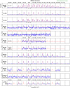 |
Fig. B.1 Spectral observations along the main cut compared to our best-fit radiative transfer model. The blue spectra show the observational data and the red spectra show the models. Each column corresponds to different offsets from the center of L 1498 according to Fig. 1. Each row shows a spectral line, except that the N2H+ (1−0) line is split into three rows corresponding to its different F1 -transition groups. The green dashed lines indicate the 3σ noise level. Observational parameters are summarized in Table 1. |
Appendix C Full ortho-H2D+ (110−111) and N2H+ (1−0) spectral line observations
We present our full o-H2D+ (110−111) spectral line observations and the N2H+ (1−0) spectral line observations obtained by Tafalla et al. (2004), comparing with our best-fit asymmetric onion-shell model.
Figures C.1 and C.2 show all the single pointing observations in black lines and models of N2H+ (1−0) and o-H2D+ (110−111) in red lines, respectively. In addition, the 3σ noise levels are denoted by green horizontal lines in Fig. C.2. The models are reproduced with our asymmetric onion-like model (Sect. 4 and Table F.1).
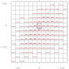 |
Fig. C.1 N2H+ (1−0) spectra from Tafalla et al. (2004). The x- and y-axes of the grid are the RA and Dec offsets with respect to the center of L 1498. Each cell shows the observational spectra as black, our modeled spectra as red, and the baselines as blue. The dimension of |

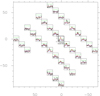 |
Fig. C.2 o-H2D+ (110−111) spectra. The x- and y-axes of the grid are the RA and Dec offsets with respect to the center of L 1498. Each cell shows the observational spectra as black, the modeled spectra as red, and the baselines as blue. The 3σ noise levels are shown in green horizontal lines. The dimensions of |

Appendix D C18O spectral line observations
We present the C18O (1−0) spectral line observations obtained by Tafalla et al. (2004) along the main cut across our model center. As the discussion in Sect. 5.1, Figure 7 indicates that the L 1498 core is embedded in an envelope consisted of a layer with AV ≈3 mag. The critical density at Tkin =10 K is 1.9 × 103 cm−3 for the J=1−0 line and 8.4 × 103 cm−3 for the J=2−1 line. Our C18O (2−1) spectral line observations shown in the bottom row in Fig. B.1 suggest that the envelope does not emit pronounced C18O (2−1) line emission compared to the core region. Therefore, the number density of the envelope should be much lower than the critical density of the J=2−1 line but slightly larger than that of the J= 1−0 line.
We find that  can reproduce the C18O (1−0) spectra without enhancing the C18O (2−1) spectra. Figure D.1 shows the single pointing observations in blue thick lines. The red C18O spectrum models are based on radiative transfer calculations performed with the asymmetric onion model (the L 1498 core) embedded in the envelope, while the black C18O (2−1) spectrum models are performed with only the asymmetric onion model of the L 1498 core. In addition, the 3σ noise levels are denoted by green dashed horizontal lines.
With  (RV = 3.1; Bohlin et al. 1978), AV =3 mag is equivalent to
  , and the thickness of the envelope is 0.46 pc (94 kau) along the line of sight with
  of 2 × 103 cm−3. For Tkin, we adopt Tkin = 10 K or the best-fit temperature from the outermost onionlike layer if it is larger than 10 K (Table F.I). Thus they are Tkin = 10 K in the southwestern envelope, and Tkin = 12 K the northeastern envelope. For X(C18O), we adopt the standard abundance of 1.7 × 10⁻⁷ (Frerking et al. 1982) except that the C18O abundance in the most northeastern region in the north-eastern envelope is decreased to the same abundance in the fifth northeastern onion-like layer as 1.9 × 10⁻⁸ in order to match the spectrum at (∆RA = 40″, ∆Dec = 40″). This lower C18O abundance may be due to the selective photodissociation at the northeastern cloud edge.
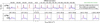 |
Fig. D.1 C180 (1−0) and (2−1) spectra along the main cut. The blue spectra show the observational data including the archival J=1−0 spectra from Tafalla et al. (2004) and our J=2−1 spectra. The black spectra show the modeled J=2−1 spectra from Fig. B.1. The red spectra show the modeled spectra of the asymmetric onion-like model embedded in an envelope that is a layer with AV =3 mag. Each column corresponds to different offsets from the center of L 1498. The green dashed lines indicate the 3σ noise level. |
Appendix E Asymmetric onion-like model
Figure E.1 shows the comparison between the spherically dissymmetric and asymmetric onion-like models. The layer width in the spherical model is chosen to be  arcsec (≈ 14.1″ and 1980 au at the distance of 140 pc), which is the same as the spacing of our IRAM 30-m/GBT pointing observations (Fig. 1). We note that the spherically dissymmetric model is comprised of two spherically symmetric models for the northeast and southwest sides with five and nine layers, respectively. We took the emission morphologies of 850 µm continuum (Fig. 2h) and the integrated intensity of N2H+ (1−0) (Fig.2i) as the reference. Since the southwest side of L 1498 is rounder than the other side, we intended to keep the southwestern geometric shape at a cross-section along the main cut and sightline (i.e., a semi-circle) the same in both symmetric and asymmetric models. We then modified the southwest side of the spherical model to become the asymmetric model by shrinking the west quadrant by a factor of 8/9, and extending the south quadrant by a factor of 9/7 along the NW–SE direction. On the northeast side, the semi-sphere extends along both the NW–SE direction and the sightline direction in order to match with the southwest side.
We choose the NW–SE axis as the x-axis (the positive direction is PA = −45°), the NE-SW axis as the y-axis (the positive direction is PA = +45°), and the line-of-sight axis as the z-axis. Supposing the radius of a layer boundary in the spherical model is rsph, then the corresponding layer boundary in the asymmetric model, rasym = (x, y, z), is defined in the four quadrants on the plane of sky by the following equations.
In the north quadrant (x > 0, y > 0),
 (E.l)
(E.l)
In the east quadrant (x < 0, y > 0),
 (E.2)
(E.2)
In the south quadrant (x < 0, y < 0),
 (E.3)
(E.3)
In the west quadrant (x > 0, y < 0),
 (E.4)
(E.4)
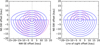 |
Fig. E.1 Comparison between the asymmetric and spherical onion-like models. The asymmetric layers are shown in the blue solid curves, while the spherical layers are shown in the magenta dashed curves. The left panel shows the cross-section of the models across the center and within the sky plane. The right panel shows the cross-section along the main cut (NE-SW direction) and the line of sight, where both asymmetric and spherical models are identical on the NE side. |
Appendix F Best-fit physical and abundance profiles
We present the best-fit quantities with their error ranges for each layer in our asymmetric onion-shell model from Fig. 4 and Fig. 6 in Table F.1.
Onion-shell model parameters.
References
- Aikawa, Y., Ohashi, N., & Herbst, E. 2003, ApJ, 593, 906 [NASA ADS] [CrossRef] [Google Scholar]
- Aikawa, Y., Herbst, E., Roberts, H., & Caselli, P. 2005, ApJ, 620, 330 [NASA ADS] [CrossRef] [Google Scholar]
- Ballesteros-Paredes, J., Klessen, R. S., Mac Low, M. M., & Vazquez-Semadeni, E. 2007, in Protostars and Planets V, eds. B. Reipurth, D. Jewitt, & K. Keil, 63 [Google Scholar]
- Beichman, C. A., Myers, P. C., Emerson, J. P., et al. 1986, ApJ, 307, 337 [NASA ADS] [CrossRef] [Google Scholar]
- Bensch, F., Stutzki, J., & Heithausen, A. 2001, A&A, 365, 285 [NASA ADS] [CrossRef] [EDP Sciences] [Google Scholar]
- Bergin, E. A., Alves, J., Huard, T., & Lada, C. J. 2002, ApJ, 570, L101 [NASA ADS] [CrossRef] [Google Scholar]
- Bernes, C. 1979, A&A, 73, 67 [NASA ADS] [Google Scholar]
- Bisschop, S. E., Fraser, H. J., Öberg, K. I., van Dishoeck, E. F., & Schlemmer, S. 2006, A&A, 449, 1297 [NASA ADS] [CrossRef] [EDP Sciences] [Google Scholar]
- Bohlin, R. C., Savage, B. D., & Drake, J. F. 1978, ApJ, 224, 132 [Google Scholar]
- Bonnell, I. A., Bate, M. R., Clarke, C. J., & Pringle, J. E. 2001, MNRAS, 323, 785 [Google Scholar]
- Bonnell, I. A., Vine, S. G., & Bate, M. R. 2004, MNRAS, 349, 735 [Google Scholar]
- Bovino, S., Ferrada-Chamorro, S., Lupi, A., et al. 2019, ApJ, 887, 224 [NASA ADS] [CrossRef] [Google Scholar]
- Bovino, S., Lupi, A., Giannetti, A., et al. 2021, A&A, 654, A34 [NASA ADS] [CrossRef] [EDP Sciences] [Google Scholar]
- Buckle, J. V., Hills, R. E., Smith, H., et al. 2009, MNRAS, 399, 1026 [Google Scholar]
- Caselli, P., Benson, P. J., Myers, P. C., & Tafalla, M. 2002, ApJ, 572, 238 [Google Scholar]
- Caselli, P., Vastel, C., Ceccarelli, C., et al. 2008, A&A, 492, 703 [NASA ADS] [CrossRef] [EDP Sciences] [Google Scholar]
- Ceccarelli, C., Caselli, P., Bockelée-Morvan, D., et al. 2014, in Protostars and Planets VI, eds. H. Beuther, R. S. Klessen, C. P. Dullemond, & T. Henning, 859 [Google Scholar]
- Chapin, E. L., Berry, D. S., Gibb, A. G., et al. 2013, MNRAS, 430, 2545 [Google Scholar]
- Crabtree, K. N., Indriolo, N., Kreckel, H., Tom, B. A., & McCall, B. J. 2011, ApJ, 729, 15 [NASA ADS] [CrossRef] [Google Scholar]
- Crapsi, A., Caselli, P., Walmsley, C. M., et al. 2005, ApJ, 619, 379 [Google Scholar]
- Daniel, F., Dubernet, M.-L., Meuwly, M., Cernicharo, J., & Pagani, L. 2005, MNRAS, 363, 1083 [NASA ADS] [CrossRef] [Google Scholar]
- Federrath, C., & Klessen, R. S. 2012, ApJ, 761, 156 [Google Scholar]
- Flower, D. R., Pineau des Forêts, G., & Walmsley, C. M. 2004, A&A, 427, 887 [NASA ADS] [CrossRef] [EDP Sciences] [Google Scholar]
- Flower, D. R., Pineau Des Forêts, G., & Walmsley, C. M. 2005, A&A, 436, 933 [NASA ADS] [CrossRef] [EDP Sciences] [Google Scholar]
- Flower, D. R., Pineau Des Forêts, G., & Walmsley, C. M. 2006, A&A, 449, 621 [NASA ADS] [CrossRef] [EDP Sciences] [Google Scholar]
- Fontani, F., Caselli, P., Crapsi, A., et al. 2006, A&A, 460, 709 [NASA ADS] [CrossRef] [EDP Sciences] [Google Scholar]
- Fontani, F., Busquet, G., Palau, A., et al. 2015, A&A, 575, A87 [NASA ADS] [CrossRef] [EDP Sciences] [Google Scholar]
- Ford, A. B., & Shirley, Y. L. 2011, ApJ, 728, 144 [NASA ADS] [CrossRef] [Google Scholar]
- Foster, J. B., & Goodman, A. A. 2006, ApJ, 636, L105 [Google Scholar]
- Frerking, M. A., Langer, W. D., & Wilson, R. W. 1982, ApJ, 262, 590 [Google Scholar]
- Fuller, G. A., & Myers, P. C. 1993, ApJ, 418, 273 [CrossRef] [Google Scholar]
- Greve, A., Kramer, C., & Wild, W. 1998, A&AS, 133, 271 [NASA ADS] [CrossRef] [EDP Sciences] [Google Scholar]
- Hennebelle, P., & Falgarone, E. 2012, A&A Rev., 20, 55 [NASA ADS] [CrossRef] [Google Scholar]
- Holdship, J., Viti, S., Jiménez-Serra, I., Makrymallis, A., & Priestley, F. 2017, AJ, 154, 38 [NASA ADS] [CrossRef] [Google Scholar]
- Holland, W. S., Bintley, D., Chapin, E. L., et al. 2013, MNRAS, 430, 2513 [Google Scholar]
- Hopkins, P. F. 2012, MNRAS, 423, 2016 [NASA ADS] [CrossRef] [Google Scholar]
- Hugo, E., Asvany, O., & Schlemmer, S. 2009, J. Chem. Phys., 130, 164302 [Google Scholar]
- Jiménez-Serra, I., Vasyunin, A. I., Spezzano, S., et al. 2021, ApJ, 917, 44 [CrossRef] [Google Scholar]
- Kirk, J. M., Ward-Thompson, D., & Crutcher, R. M. 2006, MNRAS, 369, 1445 [CrossRef] [Google Scholar]
- Kong, S., Caselli, P., Tan, J. C., Wakelam, V., & Sipilä, O. 2015, ApJ, 804, 98 [NASA ADS] [CrossRef] [Google Scholar]
- Kong, S., Tan, J. C., Caselli, P., et al. 2016, ApJ, 821, 94 [NASA ADS] [CrossRef] [Google Scholar]
- Körtgen, B., Bovino, S., Schleicher, D. R. G., Giannetti, A., & Banerjee, R. 2017, MNRAS, 469, 2602 [Google Scholar]
- Körtgen, B., Bovino, S., Schleicher, D. R. G., et al. 2018, MNRAS, 478, 95 [Google Scholar]
- Kuiper, T. B. H., Langer, W. D., & Velusamy, T. 1996, ApJ, 468, 761 [CrossRef] [Google Scholar]
- Kutner, M. L., & Ulich, B. L. 1981, ApJ, 250, 341 [NASA ADS] [CrossRef] [Google Scholar]
- Lai, S.-P., & Crutcher, R. M. 2000, ApJS, 128, 271 [NASA ADS] [CrossRef] [Google Scholar]
- Langer, W. D., & Willacy, K. 2001, ApJ, 557, 714 [NASA ADS] [CrossRef] [Google Scholar]
- Lattanzi, V., Bizzocchi, L., Vasyunin, A. I., et al. 2020, A&A, 633, A118 [NASA ADS] [CrossRef] [EDP Sciences] [Google Scholar]
- Lee, C. W., & Myers, P. C. 2011, ApJ, 734, 60 [NASA ADS] [CrossRef] [Google Scholar]
- Lee, C. W., Myers, P. C., & Tafalla, M. 1999, ApJ, 526, 788 [NASA ADS] [CrossRef] [Google Scholar]
- Lee, C. W., Myers, P. C., & Tafalla, M. 2001, ApJS, 136, 703 [NASA ADS] [CrossRef] [Google Scholar]
- Lefèvre, C., Pagani, L., Juvela, M., et al. 2014, A&A, 572, A20 [NASA ADS] [CrossRef] [EDP Sciences] [Google Scholar]
- Lefèvre, C., Pagani, L., Min, M., Poteet, C., & Whittet, D. 2016, A&A, 585, A4 [NASA ADS] [CrossRef] [EDP Sciences] [Google Scholar]
- Lemme, C., Walmsley, C. M., Wilson, T. L., & Muders, D. 1995, A&A, 302, 509 [NASA ADS] [Google Scholar]
- Levin, S. M., Langer, W. D., Velusamy, T., Kuiper, T. B. H., & Crutcher, R. M. 2001, ApJ, 555, 850 [NASA ADS] [CrossRef] [Google Scholar]
- Lin, S.-J., Pagani, L., Lai, S.-P., Lefèvre, C., & Lique, F. 2020, A&A, 635, A188 [EDP Sciences] [Google Scholar]
- Linsky, J. L. 2007, Space Sci. Rev., 130, 367 [CrossRef] [Google Scholar]
- Lique, F., Daniel, F., Pagani, L., & Feautrier, N. 2015, MNRAS, 446, 1245 [NASA ADS] [CrossRef] [Google Scholar]
- Lombardi, M., & Alves, J. 2001, A&A, 377, 1023 [NASA ADS] [CrossRef] [EDP Sciences] [Google Scholar]
- Mac Low, M.-M., & Klessen, R. S. 2004, Rev. Mod. Phys., 76, 125 [Google Scholar]
- Magalhães, V. S., Hily-Blant, P., Faure, A., Hernandez-Vera, M., & Lique, F. 2018, A&A, 615, A52 [NASA ADS] [CrossRef] [EDP Sciences] [Google Scholar]
- Mairs, S., Dempsey, J. T., Bell, G. S., et al. 2021, AJ, 162, 191 [NASA ADS] [CrossRef] [Google Scholar]
- Maret, S., Bergin, E. A., & Tafalla, M. 2013, A&A, 559, A53 [NASA ADS] [CrossRef] [EDP Sciences] [Google Scholar]
- McKee, C. F., & Ostriker, E. C. 2007, ARA&A, 45, 565 [Google Scholar]
- Möller, T., Bernst, I., Panoglou, D., et al. 2013, A&A, 549, A21 [NASA ADS] [CrossRef] [EDP Sciences] [Google Scholar]
- Mouschovias, T. C., Tassis, K., & Kunz, M. W. 2006, ApJ, 646, 1043 [Google Scholar]
- Myers, P. C., Linke, R. A., & Benson, P. J. 1983, ApJ, 264, 517 [NASA ADS] [CrossRef] [Google Scholar]
- Myers, P. C., Fuller, G. A., Goodman, A. A., & Benson, P. J. 1991, ApJ, 376, 561 [NASA ADS] [CrossRef] [Google Scholar]
- Oppenheimer, M., & Dalgarno, A. 1975, ApJ, 200, 419 [NASA ADS] [CrossRef] [Google Scholar]
- Padoan, P., Jimenez, R., Juvela, M., & Nordlund, Å. 2004, ApJ, 604, L49 [NASA ADS] [CrossRef] [Google Scholar]
- Padoan, P., Pan, L., Juvela, M., Haugbølle, T., & Nordlund, Å. 2020, ApJ, 900, 82 [NASA ADS] [CrossRef] [Google Scholar]
- Pagani, L., Salez, M., & Wannier, P. G. 1992, A&A, 258, 479 [NASA ADS] [Google Scholar]
- Pagani, L., Bacmann, A., Motte, F., et al. 2004, A&A, 417, 605 [CrossRef] [EDP Sciences] [Google Scholar]
- Pagani, L., Bacmann, A., Cabrit, S., & Vastel, C. 2007, A&A, 467, 179 [NASA ADS] [CrossRef] [EDP Sciences] [Google Scholar]
- Pagani, L., Daniel, F., & Dubernet, M.-L. 2009a, A&A, 494, 719 [NASA ADS] [CrossRef] [EDP Sciences] [Google Scholar]
- Pagani, L., Vastel, C., Hugo, E., et al. 2009b, A&A, 494, 623 [NASA ADS] [CrossRef] [EDP Sciences] [Google Scholar]
- Pagani, L., Ristorcelli, I., Boudet, N., et al. 2010, A&A, 512, 3 [Google Scholar]
- Pagani, L., Roueff, E., & Lesaffre, P. 2011, ApJ, 739, L35 [NASA ADS] [CrossRef] [Google Scholar]
- Pagani, L., Bourgoin, A., & Lique, F. 2012, A&A, 548, L4 [NASA ADS] [CrossRef] [EDP Sciences] [Google Scholar]
- Pagani, L., Lesaffre, P., Jorfi, M., et al. 2013, A&A, 551, A38 [NASA ADS] [CrossRef] [EDP Sciences] [Google Scholar]
- Pagani, L., Lefèvre, C., Juvela, M., Pelkonen, V. M., & Schuller, F. 2015, A&A, 574, L5 [NASA ADS] [CrossRef] [EDP Sciences] [Google Scholar]
- Pagani, L., Frayer, D., Pagani, B., & Lefèvre, C. 2020, A&A, 643, A126 [NASA ADS] [CrossRef] [EDP Sciences] [Google Scholar]
- Pineau des Forêts, G., Flower, D. R., & McCarroll, R. 1991, MNRAS, 248, 173 [NASA ADS] [Google Scholar]
- Pineda, J. L., Goldsmith, P. F., Chapman, N., et al. 2010, ApJ, 721, 686 [NASA ADS] [CrossRef] [Google Scholar]
- Priestley, F. D., Viti, S., & Williams, D. A. 2018, AJ, 156, 51 [NASA ADS] [CrossRef] [Google Scholar]
- Priestley, F. D., Yin, C., & Wurster, J. 2022, MNRAS, 515, 5689 [NASA ADS] [CrossRef] [Google Scholar]
- Shirley, Y. L., Nordhaus, M. K., Grcevich, J. M., et al. 2005, ApJ, 632, 982 [NASA ADS] [CrossRef] [Google Scholar]
- Shu, F. H., Adams, F. C., & Lizano, S. 1987, ARA&A, 25, 23 [Google Scholar]
- Steinacker, J., Pagani, L., Bacmann, A., & Guieu, S. 2010, A&A, 511, A9 [NASA ADS] [CrossRef] [EDP Sciences] [Google Scholar]
- Steinacker, J., Andersen, M., Thi, W. F., et al. 2015, A&A, 582, A70 [NASA ADS] [CrossRef] [EDP Sciences] [Google Scholar]
- Stutz, A. M., Rieke, G. H., Bieging, J. H., et al. 2009, ApJ, 707, 137 [Google Scholar]
- Tafalla, M., Myers, P. C., Caselli, P., Walmsley, C. M., & Comito, C. 2002, ApJ, 569, 815 [Google Scholar]
- Tafalla, M., Myers, P. C., Caselli, P., & Walmsley, C. M. 2004, A&A, 416, 191 [NASA ADS] [CrossRef] [EDP Sciences] [Google Scholar]
- Tafalla, M., Santiago-García, J., Myers, P. C., et al. 2006, A&A, 455, 577 [NASA ADS] [CrossRef] [EDP Sciences] [Google Scholar]
- Tassis, K., & Mouschovias, T. C. 2004, ApJ, 616, 283 [Google Scholar]
- Tokuda, K., Fujishiro, K., Tachihara, K., et al. 2020, ApJ, 899, 10 [NASA ADS] [CrossRef] [Google Scholar]
- Vázquez-Semadeni, E., González-Samaniego, A., & Colín, P. 2017, MNRAS, 467, 1313 [NASA ADS] [Google Scholar]
- Vázquez-Semadeni, E., Palau, A., Ballesteros-Paredes, J., Gómez, G. C., & Zamora-Avilés, M. 2019, MNRAS, 490, 3061 [Google Scholar]
- Walmsley, C. M., Flower, D. R., & Pineau des Forêts, G. 2004, A&A, 418, 1035 [NASA ADS] [CrossRef] [EDP Sciences] [Google Scholar]
- Wannier, P. G. 1980, ARA&A, 18, 399 [NASA ADS] [CrossRef] [Google Scholar]
- Weingartner, J. C., & Draine, B. T. 2001, ApJ, 548, 296 [Google Scholar]
- Willacy, K., Langer, W. D., & Velusamy, T. 1998, ApJ, 507, L171 [NASA ADS] [CrossRef] [Google Scholar]
- Wilson, T. L., & Rood, R. 1994, ARA&A, 32, 191 [Google Scholar]
- Wolkovitch, D., Langer, W. D., Goldsmith, P. F., & Heyer, M. 1997, ApJ, 477, 241 [NASA ADS] [CrossRef] [Google Scholar]
- Yin, C., Priestley, F. D., & Wurster, J. 2021, MNRAS, 504, 2381 [NASA ADS] [CrossRef] [Google Scholar]
- Young, K. E., Lee, J.-E., Evans, Neal J., I., Goldsmith, P. F., & Doty, S. D. 2004, ApJ, 614, 252 [Google Scholar]
Vturb is defined as the 3D isotropic nonthermal velocity dispersion. If Tkin and Vturb are constant along the line of sight, the FWHM of the line profile is given by  , where kB is the Boltzmann constant and m is the mass of the observed species.
P * Tb = ∫∫2π P(θ, ϕ)Tb,(θ − θ0, ϕ − ϕ0) dΩ with the telescope pointing toward the direction of (θ0, ϕ0).
Bensch et al. (2001) introduced TMBC = PMB * Tb/ΩMB as the “corrected main beam temperature” to exclude the error beam contributions (PEB) in contrast to the common main beam temperature definition of TMB = P* Tb/ΩMB. We can see that TMB will be over-corrected (TMB,C < TMB) with non-negligible PEB.
All Tables
All Figures
|
Fig. 1 Multi-pointing grids overlaid with the SCUBA-2850 µm map. The black dots in a (∆RA, ∆Dec)=(10″, 10″)-spacing 45º-cut show the pointings of IRAM 30-m and GBT observations. The red dotted grid shows the pointings of JCMT observations. The circles at the top and bottom indicate the beam sizes (θMB) of each spectral observation with the same color as the pointing grid except that GBT beam sizes are shown in blue. The 850 µm map is shown in grayscale with a beam size of 14″ and overlaid with its contours at 0%, 20%, 40%, 60%, and 80% of its peak intensity at 78 mJy beam−1. |
| In the text | |
|
Fig. 2 L 1498 maps of continuum, extinction, and line integrated intensity. The CFHT NIR maps at the (a) J band, (b) H band, and (c) Ks band. Spitzer MIR maps at (d) IRAC1 band, (e) IRAC2 band, and (f) IRAC4 band with its contours at 7.0 MJy sr−1. (g) Visual extinction map with a beam size of 50″ with contours at 2.5, 5, 10, 15, 20, 25 mag. (h) JCMT SCUBA-2 850 µm map with a beam size of 14″ and the contours shown in Fig. 1. (i) Integrated intensity maps of N2H+ J=1–0 from Tafalla et al. (2004), calculated within VLSR=[−0.5 km s−1, 15.2 km s−1] with its contours at 20, 40, 60, 80% of its peak at 2.5 K km s−1 and a beam size of 26″. The central cross in each panel indicates the center of L 1498. The scale bars of 0.05 pc and AV/millimeter-wavelength beam sizes are denoted in the bottom right and bottom left corners, respectively. |
| In the text | |
|
Fig. 3 Onion-like physical models. (a) The spherical model with the layer width as |
| In the text | |
|
Fig. 4 Physical and abundance profiles along the main cut. The profiles of number density ( |
| In the text | |
|
Fig. 5 Chemical modeling of the abundance ratio of N2D+/N2H+ and the abundances of o-H2D+ and DCO+ for each layer. Left and right columns: chemical model solutions (curves) and the observationally derived values (horizontal lines). Middle column: observationally derived profiles with uncertainties from Fig. 4. The model solutions and observed values are color-coded by different layers. The models are calculated with an initial OPR(H2) of 3, a cosmic ray ionization rate (ξ) of 3 × 10⁻¹⁷ s−1, and an average grain radius (agr) profile shown in Fig. 6. The two dashed-dotted vertical lines in each panel indicate a time range for which the model values cross the observations within their error bars, and we make such model curves thicker. The thick model curve is displayed as dashed if the observation only has an upper limit. The solid vertical line indicates the lower limit on the core age of L 1498 as 0.16 Ma. |
| In the text | |
|
Fig. 6 Profiles of the abundances CO, N2, and the grain radius (agr). The X(12CO), X(N2), and agr profiles are the best-fit results from the chemical modeling. The X(C18O) profile is obtained by assuming a 12CO/C18O abundance ratio of 560 or a constant value of 1.9 × 10⁻⁸. |
| In the text | |
|
Fig. 7 Comparison of the NICER-derived AV profile and the AV profile derived from the column density from the best-fit asymmetric onion-like model along the main cut. The black crosses are the NICER-derived AV values at each pixel in the 50″-wide strip on the AV map shown as the insert. The orange and red squares with error bars show the radially averaged AV profile with the 14.1″-bin from the strip, where the central region is represented as lower limits due to the lack of the Ks-band detections. The gray step curve shows the AV profiles converted from our onion-like model, while the blue step curve is convolved with the AV-beam of 50″. The coverage of our onion-like model is shown by black dashed lines. The insert shows the NICER-derived AV map with the 50″-beam (Fig. 2g) overlaid with black dots, indicating the stars only detected in the IRAC1/2 bands but with the artificial Ks-band detection (see Sect. 4.4). |
| In the text | |
|
Fig. B.1 Spectral observations along the main cut compared to our best-fit radiative transfer model. The blue spectra show the observational data and the red spectra show the models. Each column corresponds to different offsets from the center of L 1498 according to Fig. 1. Each row shows a spectral line, except that the N2H+ (1−0) line is split into three rows corresponding to its different F1 -transition groups. The green dashed lines indicate the 3σ noise level. Observational parameters are summarized in Table 1. |
| In the text | |
|
Fig. C.1 N2H+ (1−0) spectra from Tafalla et al. (2004). The x- and y-axes of the grid are the RA and Dec offsets with respect to the center of L 1498. Each cell shows the observational spectra as black, our modeled spectra as red, and the baselines as blue. The dimension of |
| In the text | |
|
Fig. C.2 o-H2D+ (110−111) spectra. The x- and y-axes of the grid are the RA and Dec offsets with respect to the center of L 1498. Each cell shows the observational spectra as black, the modeled spectra as red, and the baselines as blue. The 3σ noise levels are shown in green horizontal lines. The dimensions of |
| In the text | |
|
Fig. D.1 C180 (1−0) and (2−1) spectra along the main cut. The blue spectra show the observational data including the archival J=1−0 spectra from Tafalla et al. (2004) and our J=2−1 spectra. The black spectra show the modeled J=2−1 spectra from Fig. B.1. The red spectra show the modeled spectra of the asymmetric onion-like model embedded in an envelope that is a layer with AV =3 mag. Each column corresponds to different offsets from the center of L 1498. The green dashed lines indicate the 3σ noise level. |
| In the text | |
|
Fig. E.1 Comparison between the asymmetric and spherical onion-like models. The asymmetric layers are shown in the blue solid curves, while the spherical layers are shown in the magenta dashed curves. The left panel shows the cross-section of the models across the center and within the sky plane. The right panel shows the cross-section along the main cut (NE-SW direction) and the line of sight, where both asymmetric and spherical models are identical on the NE side. |
| In the text | |
Current usage metrics show cumulative count of Article Views (full-text article views including HTML views, PDF and ePub downloads, according to the available data) and Abstracts Views on Vision4Press platform.
Data correspond to usage on the plateform after 2015. The current usage metrics is available 48-96 hours after online publication and is updated daily on week days.
Initial download of the metrics may take a while.