| Issue |
A&A
Volume 688, August 2024
|
|
|---|---|---|
| Article Number | A26 | |
| Number of page(s) | 16 | |
| Section | Interstellar and circumstellar matter | |
| DOI | https://doi.org/10.1051/0004-6361/202449745 | |
| Published online | 02 August 2024 | |
The asymmetric bipolar [Fe II] jet and H2 outflow of TMC1A resolved with the JWST NIRSpec Integral Field Unit
1
Department of Astronomy, University of Virginia,
Charlottesville,
VA
22903,
USA
e-mail: This email address is being protected from spambots. You need JavaScript enabled to view it.
2
Institute of Astronomy, Department of Physics, National Tsing Hua University,
Hsinchu,
Taiwan
3
Chalmers University of Technology, Department of Space, Earth and Environment,
412 96
Gothenburg,
Sweden
4
Jet Propulsion Laboratory, California Institute of Technology,
4800 Oak Grove Drive,
Pasadena,
CA
91109,
USA
5
Leiden Observatory, Leiden University,
PO Box 9513,
2300RA
Leiden,
The Netherlands
6
Niels Bohr Institute, University of Copenhagen,
Øster Voldgade 5–7,
1350
Copenhagen K.,
Denmark
7
National Radio Astronomy Observatory,
520 Edgemont Road,
Charlottesville,
VA
22903,
USA
Received:
26
February
2024
Accepted:
23
April
2024
Abstract
Context. Protostellar outflows exhibit large variations in their structure depending on the observed gas emission. To understand the origin of the observed variations, it is important to analyze the differences in the observed morphology and kinematics of the different tracers. The James Webb Space Telescope (JWST) allows us to study the physical structure of the protostellar outflow through well-known near-infrared shock tracers in a manner unrivaled by other existing ground-based and space-based telescopes at these wavelengths.
Aims. This study analyzes the atomic jet and molecular outflow in the Class I protostar, TMC1A, utilizing spatially resolved [Fe II] and H2 lines to characterize the morphology and to identify previously undetected spatial features, and compare them to existing observations of TMC1A and its outflows observed at other wavelengths.
Methods. We identified a large number of [Fe II] and H2 lines within the G140H, G235H, and G395H gratings of the NIRSpec IFU observations. We analyzed their morphology and position-velocity (PV) diagrams. From the observed [Fe II] line ratios, the extinction toward the jet is estimated.
Results. We detected the bipolar Fe jet by revealing, for the first time, the presence of a redshifted atomic jet. Similarly, the red-shifted component of the H2 slower wide-angle outflow was observed. The [Fe II] and H2 redhifted emission both exhibit significantly lower flux densities compared to their blueshifted counterparts. Additionally, we report the detection of a collimated high-velocity (~100 km s−1), blueshifted H2 outflow, suggesting the presence of a molecular jet in addition to the well-known wider angle low-velocity structure. The [Fe II] and H2 jets show multiple intensity peaks along the jet axis, which may be associated with ongoing or recent outburst events. In addition to the variation in their intensities, the H2 wide-angle outflow exhibits a ring-like structure. The blueshifted H2 outflow also shows a left-right brightness asymmetry likely due to interactions with the surrounding ambient medium and molecular outflows. Using the [Fe II] line ratios, the extinction along the atomic jet is estimated to be between AV = 10–30 on the blueshifted side, with a trend of decreasing extinction with distance from the protostar. A similar AV is found for the redshifted side, supporting the argument for an intrinsic red-blue outflow lobe asymmetry rather than environmental effects such as extinction. This intrinsic difference revealed by the unprecedented sensitivity of JWST, suggests that younger outflows already exhibit the red-blue side asymmetry more commonly observed toward jets associated with Class II disks.
Key words: atomic data / molecular data / methods: data analysis / techniques: imaging spectroscopy / stars: jets / stars: protostars
© The Authors 2024
 Open Access article, published by EDP Sciences, under the terms of the Creative Commons Attribution License (https://creativecommons.org/licenses/by/4.0), which permits unrestricted use, distribution, and reproduction in any medium, provided the original work is properly cited.
This article is published in open access under the Subscribe to Open model. This email address is being protected from spambots. You need JavaScript enabled to view it. to support open access publication.
1 Introduction
Protostellar outflows are an integral part of star formation, transporting material, momentum, and energy from the protostar and accretion disk, and contributing to the redistribution of mass and angular momentum throughout the protostellar system (e.g Frank et al. 2014; Myers et al. 2023; Pascucci et al. 2023). There is a great deal of diversity in the structure, strength, and even presence of atomic and molecular emission lines in protostellar outflows, alluding to a possible diversity in the launching mechanisms (e.g. Arce et al. 2007; Seale & Looney 2008; Bally 2016; Tychoniec et al. 2019). One way to improve our understanding of protostellar outflows is by analyzing spatially resolved near-IR atomic and molecular emission along the protostellar outflow using state-of-the-art instruments such as the James Webb Space Telescope (JWST).
Most protostellar outflows are observed to be bipolar (e.g. Shu & Adams 1987; Frank 1999; Bally et al. 2007; Seale & Looney 2008; Bally 2016), but are often asymmetric in their brightness and morphology (e.g. Mundt et al. 1990; Ray et al. 1996, 2007; White et al. 2014; Bally 2016). It is still not understood whether observed differences in the sides and/or lobes of bipolar outflows are due to intrinsic differences in the strengths (which we correlate with brightness) of the outflows or due to extrinsic factors such as a nonuniform ambient medium. There have been several attempts to explain these asymmetries around more evolved (Class II) sources. For example, in the case of FS Tauri B, Liu et al. (2012) suggested that the difference in mass-loss rate found in the bipolar outflow lobes is a result of the system maintaining linear momentum balance, which results in the lobe with lower mass having a higher velocity. In the case of DG Tauri B, Podio et al. (2011) suggested that the bipolar asymmetry is due to the interaction of the bipolar outflow with an asymmetric ambient medium, while White et al. (2014) proposed that the outflow might be intrinsically symmetric, and that the observed asymmetry is caused by environmental effects such as obscuration by an asymmetric ambient medium. Furthermore, asymmetries between the two bipolar lobes have been observed in a number of Class II sources, such as AW Aurigae (e.g. Woitas et al. 2002) and TH 28 (e.g. Melnikov et al. 2023). With JWST we can establish whether such an asymmetry is observed toward the more deeply embedded protostars.
Protostellar outflows that are collimated and travel at velocities greater than ~100 km s−1 are called protostellar jets (e.g. Bally 2016; Ray et al. 2023). While jets are observed at all evolutionary stages in protostellar systems with active accretion, their overall strengths and the presence of collimated, fast, molecular components tend to decline with age (e.g. Bontemps et al. 1996; Reipurth & Bally 2001; Cabrit et al. 2011; Bally 2016; Podio et al. 2021). Molecular jets are typically associated with younger protostellar sources such as the deeply embedded Class 0 proto-star HH 211, where a fast (~100 km s−1) H2 jet was found (Ray et al. 2023), in addition to a knotty and bipolar jet in SiO (Lee et al. 2018). However, a deeply embedded atomic jet in [Fe II], [S I], and [S II] has also been detected in HH 211 with Spitzer (Dionatos et al. 2010). An embedded jet is also detected in the Class 0 protostar L1448-C, but the atomic lines are less bright and carry less overall mass flux than their molecular counterparts (Dionatos et al. 2009; Nisini et al. 2015). In more evolved Class I sources, atomic jets tend to be observed carrying more mass flux at higher velocities and at larger scales than the molecular jets (Davis et al. 2003; Nisini et al. 2005; Podio et al. 2006; Sperling et al. 2021). Finally, in Class II sources, the jet as a whole becomes fainter, and only the atomic component is found to still be well collimated (Hartigan et al. 1995; Hirth et al. 1997), while the molecular component is slower and no longer well collimated (Beck et al. 2008; Agra-Amboage et al. 2014).
These observed trends may point to the survival of molecules in the jet such as H2 in deeply embedded Class 0 protostars due to shielding by dust (e.g., Cabrit et al. 2011; Panoglou et al. 2012; Tabone et al. 2020). As the protostellar system evolves, the mass accretion rate onto the protostar decreases, the protostel-lar envelope dissipates, and ultraviolet (UV) photons from the star may destroy most of the molecules. Alternatively, it might be possible that when infall is highest near the beginning of the star formation process, the launched outflows may be denser and slower, resulting in weaker shocks where molecules can survive or reform more easily.
Along with the atomic and molecular jets, large-scale spatial brightness variations along protostellar jets, typically referred to as “knots”, have been observed. Along with shocks, these knots have historically been designated as Herbig-Haro (HH) objects (e.g. Herbig 1951; Haro 1952; Reipurth & Bally 2001). Knots are usually explained as either high-velocity jet material colliding with the slower surrounding molecular gas or older, slower outflow material, creating shock fronts (e.g. Mundt & Fried 1983). A well-studied example is the HH 111 complex which shows a high-velocity [S II] and Hα jet (e.g. Reipurth et al. 1997) and high-velocity (~400–500 km s−1) molecular CO “bullets” (Cernicharo & Reipurth 1996) in addition to H2 knots situated between the other components and the bow shock structure (Gredel 1994). The CO bullets and H2 knots are thought to be the dense material trapped between the radiative shocks that has cooled sufficiently to form molecules (Reipurth & Heathcote 1997; Melnick & Kaufman 2015; Godard et al. 2019).
The JWST provides unprecedented access to near- and mid-infrared wavelengths that are home to many atomic and molecular lines, including forbidden [Fe II] and rotational H2 emission lines known to be shock tracers (e.g. Giannini et al. 2013; Reipurth et al. 2019; Fedriani et al. 2019; Harsono et al. 2023; Federman et al. 2024; Beuther et al. 2023; Tychoniec et al. 2021; Delabrosse et al. 2024; Nisini et al. 2024). Specifically, the NIRSpec Integral Field Unit (IFU) (Jakobsen et al. 2022; Böker et al. 2022) on JWST covers a ~3 × 3″ field of view (FOV) with a 0.″1 spatial resolution, providing a high-quality spectrum at each spaxel. The NIRSpec IFU has already proven a valuable instrument for revealing previously undetected jets in Class 0/1 sources such as IRAS 16253-2429 (Narang et al. 2024) and TMC1A (Harsono et al. 2023). Previous JWST-NIRSpec studies have primarily focused on longer wavelength [Fe II] lines such as 4.11 and 4.89 µm with the G395M/H gratings, and the 5.34 and 17.89 µm lines with the MIRI Medium Resolution Spectrometer (MRS) (Rieke et al. 2015; Wright et al. 2015; Yang et al. 2022). However, there are numerous [Fe II] lines in the 1–2 µm region that can be used to trace shocks and excitation conditions (Giannini et al. 2008, 2013, 2015; Koo et al. 2016).
The Class I low-mass protostar TMC1A, observed with NIRSpec IFU from 1 to 5 µm inclusive, presents a great opportunity to investigate the above-mentioned emission lines that trace shocks of both atomic and molecular outflows. Additional data is also available as the molecular outflow of TMC1A has been observed by the Atacama Large Millimeter/sub-millimeter Array, in particular the outflow traced by the rotational transitions of 12CO and its isotopologs (e.g. Chandler et al. 1996; Aso et al. 2015, 2021; Bjerkeli et al. 2016). Comparing the different outflow components observed in a single source (such as TMC1A) provides an opportunity to discover how these components differ in terms of kinematics and location.
For this study we conducted a thorough search for [Fe II] and H2 emission lines using JWST’s NIRSpec IFU, and explored the spatial and kinematic characteristics (e.g. morphology) of the atomic iron jet and molecular H2 outflow associated with the Class I protostar, TMC1A (IRAS 04365+2535, with a distance of 140 pc, Galli et al. 2019). In Sect. 2, we describe the observations and data reduction used in our analysis. In Sect. 3.1, we discuss the characteristics of the detected [Fe II] and H2 lines. In Sects. 3.2 and 3.3, we examine the morphology of the [Fe II] and H2 lines. In Sect. 3.4, we estimate the line-of-sight extinction toward the jet using the [Fe II] lines. In Sect. 4, we discuss the implications of our results in the context of protostellar outflows. Finally, in Sect. 5, we summarize our results and list our conclusions on the morphology and asymmetries observed in the atomic and molecular outflows.
2 Observations and data reduction
JWST-NIRSpec observations of TMC1A were first presented in Harsono et al. (2023) (PID: 2104, PI: Harsono), and we refer to that paper for the observational details. Here, we focus our analysis on the 1–5 µm [Fe II] and H2 emission lines. We used the Atomic Line List version:3.00b5 database (van Hoof 2018) and the NIST Atomic Spectra Database (Kramida et al. 2023) to find the physical properties of each [Fe II] transition (rest wavelengths, Einstein A coefficients, energy levels), and the Gemini H2 line list to obtain the corresponding information for the H2 lines. The velocity of the line emission in each spaxel was determined relative to the vacuum rest wavelengths and calculated using the formula  , where λ0 represents the rest wavelength and c is the speed of light. We adopted the rest wavelengths in the Atomic Line List Database for the [Fe II] lines, although we note that differences in the rest wavelength can lead to different velocities.
In Harsono et al. (2023), the Stage 3 pipelined products were generated with JWST pipeline v1.9.6 (Bushouse et al. 2023a). In this study, we used v1.11.4 pipeline (Bushouse et al. 2023b) and have re-calibrated the raw JWST data using the updated calibration files JWST_1123.PMAP (Greenfield & Miller 2016). The new pipeline has improved upon the snowball artifact that is caused by the cosmic rays and its flagging routines for outlier detections. Furthermore, a large improvement in flux calibration was seen between V1.9.6 and v1.11.4. Following Harsono et al. (2023) and Sturm et al. (2023), the outlier detection step was skipped during the Stage 3 pipeline as it tends to flag out strong lines and the saturated central pixel extensively. After inspecting the final spectral cubes, we manually masked the bad spaxels after performing continuum subtraction and applying signal-to-noise constraints.
In Fig. 1, we show a series of integrated emission (moment 0) maps, centered on the [Fe II] line at 1.644 µm to illustrate each step of the data reduction process (above and beyond the JWST pipeline). First, we fitted the continuum independently in each spaxel within a spectral window near the rest wavelength of each emission line of interest using a linear polynomial fit (Fig. 1B). We then subtracted this fit from the data in each spaxel to obtain a continuum-subtracted data cube (Fig. 1C). Following this, we estimated the noise in each spaxel across the spectral cube by adding together the 1-sigma flux error obtained from the pipeline with a calibration flux error of 5% in each spaxel (see JWST User Documentation) and performed a signal-to-noise ratio (S/N) cut to select only data above a threshold (S /N≥3), and masked values below the threshold by setting them to a small value (10−32) (Fig. 1D.). Bad spaxels (Böker et al. 2023) appear as delta functions with very large intensities in the spectral dimension. We manually inspected the data to flag these bad spaxels (Fig. 1E). As seen in the fourth column (D) in Fig. 1, the location of bad spaxels can differ depending on the wavelength and the location of the spatial mask had to be accommodated accordingly.
We explored several methods for performing the continuum subtraction, for example median filters, linear fitting, and taking the average median value of the continuum away from the line. We adopted the linear fitting method because the median filter is sensitive to the size of the kernel and dependent on the wavelength, while the averaging of the median values away from the line does not account for the general increasing trend of the continuum with wavelength, which can be significant from one side of the line to the other. Differentiating between emission lines and the continuum poses a difficult challenge near the pro-tostar as the continuum is much brighter thus decreasing the line-to-continuum ratio (i.e. <50–100 AU from the protostar in our observations). The issue of contamination due to scattered light is also less significant in the regions far from the protostar since the continuum intensity is much lower. As a result, much of our analysis avoided focusing on the region near the protostar.
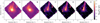 |
Fig. 1 Illustration of the data reduction process for the 1.644 µm [Fe II] line. (A) Integrated flux density maps (moment 0) of the line after the pipeline. (B) Result of the continuum fit. (C) Continuum-subtracted emission map. (D) Continuum-subtracted map with an S/N cut (Fλ ≥ 3). (E) Zeroth moment map after removal of bad spaxels. |
3 Results: The atomic and molecular outflows
In this section, we describe our detections and analysis of the [Fe II] and H2 lines. For each of the strong lines, we analyzed their morphology by comparing their flux density maps, spectral line profiles, and position-velocity (PV) diagrams. Finally, we used these results to estimate the extinction along the jet.
3.1 [Fe II] and H2 detections
We detect a total of 30 forbidden [Fe II] emission lines to the north of the protostar (the blueshifted region) between 1 and 5.3 µm (see Sect. 3.2). The spectra and peak line flux density maps (in units of µJy) for all detected transitions are presented in Figs. 2 and 3, respectively. The spectra in Fig. 2 were extracted from a single spaxel (see black cross in the 1.644 µm panel of Fig. 3) where the continuum and scattered light contamination is at a minimum while still recovering the fainter lines. The peak flux density maps are shown in Fig. 3, where the velocity of each map matches with the velocity of the peak flux density for each line shown in Fig. 2. We found that this approach allows for the clearest distinction of the extended structure of the blueshifted jet. We note that the 4.889 µm [Fe II] line is contaminated by strong CO fundamental (v = 1–0) ro-vibrational emission closer to the protostar. As a workaround, the spectrum of this particular line is extracted from a spaxel at a larger offset (cf. the location of the cross in the 4.889 µm panels in Fig. 3). The [Fe II] detections include lines originating from the a2G, a4D, a4P, a2P, and a2H levels, with upper energies ranging from 2430–26 055 K. The details of each line and the observed line ratio with respect to the 1.644 µm line are reported in Appendix A.
In Figs. 4 and 5, we present the 26 H2 emission lines that we detect. Figure 4 shows the 1D spectra for a bright spaxel in the north-east section of the H2 outflow (see the black cross in the 2.122 µm map in Fig. 5). The chosen spaxel is taken from one of the brightest regions of the H2 outflow. This location also benefits from being far from the protostar to minimize contamination from the bright scattered dust continuum. The continuum is stronger at wavelengths > 2 µm compared to the 1–2 µm range, where most of the [Fe II] lines are detected. As was done for [Fe II], the flux density maps in Fig. 5 are shown at the velocities given by the peak line intensities in Fig. 4. The H2 lines detected include the S, Q, and O rotational transition branches, with upper energies spanning from 6000 K to 17 500 K. The details of each line and the observed line ratio with respect to the 2.122 µm line are reported in Appendix A.
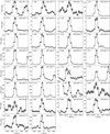 |
Fig. 2 Detected [Fe II] emission lines in order of increasing wavelength. Each panel shows a spectrum taken in the northern part of the outflow along the jet axis (~0.5 arcsec away from the protostar). The location of the spaxel is shown as a cross (×) in the panel of the 1.644 µm line of Fig. 3. Meanwhile, the 4.889 µm spectrum is extracted from a location that is marked by the cross in the panel for the 4.889 µm in Fig. 3 to avoid the contamination by the CO fundamental ro-vibrational line. Velocities are calculated independently for each line with respect to the rest wavelength (see Table A.1). The wavelength in microns is given in the upper left of each panel, and the transition terms are given in the upper right and summarized in Table A.1. The 1.749 µm line is blended with the H2 1–0 S(7) line and each is labeled in the inset. Similarly the Br 18 hydrogen recombination line is denoted in the 1.534 µm line. The 1σ uncertainty including a 5% calibration uncertainty is shown by the shaded region. |
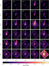 |
Fig. 3 Each panel shows the peak flux density map of the detected [Fe II] lines with an S /N ≥ 3 and bad pixels masked out. The black cross (×) with white borders in the panel for the 1.644 µm line denotes the spaxel used to extract the 1D spectra in Fig. 2. A different spaxel is used to extract the 4.89 µm line profile since it is affected by contamination closer to the protostar. The redshifted or southern part of the outflow discussed in later sections (see Sect. 3.2) does not appear in these maps since we plotted the flux density maps at the velocity corresponding to the peak line flux for a spaxel located in the blueshifted side of the jet. The rest wavelength in microns of each line is overplotted in the upper left of each panel. |
3.2 The bipolar atomic jet
We investigated the spatial and velocity structure of the bright 1.644 µm [Fe II] line to characterize the atomic jet emanating from TMC1A. Harsono et al. (2023) revealed a bright blueshifted atomic jet to the northern side of the protostar in TMC1A. In addition to this blueshifted component, we detect a dimmer redshifted component of the jet on the southern side of the protostar in the 1.257, 1.644 and 1.803 µm lines, the first indication that the atomic jet in TMC1A is bipolar.
In Fig. 6, we show the flux density maps of the 1.644 µm [Fe II] line across several velocity bins, overlaid with contours at several flux levels with signal-to-noise greater than 3. At 1.644 µ m, the width of each velocity bin is approximately 40 km s−1. The flux density of the blueshifted component peaks at around −70 km s−1, with emission detected at velocities upward of approximately −150 km s−1. The redshifted side, although it is 10–30× dimmer than the blueshifted side, has its peak flux density at a velocity of ~190 km s−1 with tentative evidence of high-velocity components close to ~230 km s−1. However, the highest velocity components of the redshifted outflow are only found close to the edge of the IFU FOV, and need confirmation with additional observations.
Due to the protostar being offset from the center of the FOV of our observations, more of the blueshifted jet is within the FOV, and because the blueshifted jet is substantially brighter, we detect spatially distinct features in the flux density maps. The structure of the atomic jet is characterized by a distinctive peak in the flux density profile coinciding with the apparent jet axis, with a sharp decrease appearing on each side. To highlight the location of the peaks, we took 1D slices of the flux density maps along the axis of the [Fe II] jet and normalized the flux density at the highest velocity component of the jet (Fline) to the continuum flux density at that velocity (Fcont). This shows the flux density of the fastest component of the jet for the 1.644 µm line in terms of its strength in comparison to the continuum and makes it easier to determine the location of the peaks.
Within the FOV of these observations, we identify three distinct intensity peaks visible in the brightest [Fe II] lines (e.g., 1.257, 1.644, 1.810 µm) on the northern side of the atomic jet, as shown in Fig. 7. For brevity, we only show the 1.644 µm line and note that the location of the peaks does not change significantly in the other lines. We determined the location of these peaks by fitting Gaussian profiles to the normalized 1D flux density profiles. The distances of each peak are reported in AU from the central star and de-projecting each point along the jet adopting an inclination with respect to the plane of the sky of ~35º for the jet, based on the disk inclination of ~55º (where 90º would be edge-on) (Harsono et al. 2021).
The first peak (1F) appears as as an extended structure with a maximum in its flux density profile at a de-projected distance of ~200 AU (see Fig. 7). The second emission feature (2F) is only visible in the brighter [Fe II] lines and is considerably smaller than the other two, located at a distance of approximately 270 AU from the protostar. The third emission feature (3F) is observed in several [Fe II] lines and is located close to the edge of the FOV at ~370 au from the protostar. Adopting a de-projected line-of-sight tangential velocity υgas = υobs/ sin(35º) = −150 km s−1/sin(35º) ≈ −260 km s−1, the location of these peaks correspond to dynamical timescales  of 4, 5, and 7 yr, respectively, implying a ~1–2 yr dynamical time difference between adjacent peaks.
We employed position-velocity (PV) diagrams to examine velocity profiles perpendicular the jet axis for each distinct emission feature in the bright 1.644 µm line (Fig. 8, top row).
Utilizing the Astropy PV Extractor, we constructed PV diagrams by defining a line perpendicular to the jet axis with a width of 3 pixels, and the velocity space was computed using the rest wavelength of the line. Solid white dots overlaid on the diagrams represent velocities at the peak line flux density. At this spectral resolution, no clear indication of a velocity gradient can be discerned. Theoretically, protostellar outflows are expected to rotate, and indeed there is evidence to support it (e.g. Frank et al. 2014). We would expect the rotation to show up as an increasing or decreasing velocity gradient perpendicular to the jet axis, as seen in some sources (e.g., DG Tau, Zapata et al. 2015; De Valon et al. 2020). In these observations, the velocity at peak flux density remains constant across the jet axis within the velocity resolution and does not change significantly from one peak to the next.
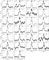 |
Fig. 4 Line profiles of the detected H2 emission lines in order of increasing wavelength. Each spectrum was taken in the northern part of the outflow marked by the black cross (×) in the 2.122 µm panel of Fig. 5. This location was chosen because this region is bright in H2, while the contamination from scattered light that is worse at longer wavelengths is minimized, easing the detection of weaker line emission. |
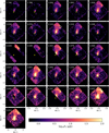 |
Fig. 5 Peak flux density maps of the detected H2 lines similar to Fig. 3. The black cross (×) with white borders in the 2.122 µm panel corresponds to the spaxel where the spectra in Fig. 4 were taken. |
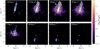 |
Fig. 6 Channel maps of the 1.644 µm [Fe II] line. Contours are plotted at 1.5, 2.5, 5, and 15 µJy. |
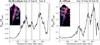 |
Fig. 7 Peaks in the [Fe II] (left) and H2 (right) outflows. The flux density profile of the highest velocity emission as a function of the deprojected distance along the jet’s axis (−150 km s−1 for [Fe II], −110 km s−1 for H2) is shown normalized with respect to the dust continuum. The inset in each panel shows the flux density maps with color maps logarithmically spaced from 10−2 to 10 µJy. The dashed vertical lines correspond to the peak (central) position of each peak determined by fitting Gaussian profile to the flux density profile (Fline/Fcont vs distance). The same locations are indicated by the white dashed lines in the flux density map in the inset. |
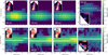 |
Fig. 8 PV diagrams of the 1.644 µm [Fe II] (top row) and 2.803 µm H2 (bottom row) lines at different locations in the bipolar jet. The distance offset from the jet axis is calculated by adopting a distance of 140 pc without de-projection since the slices are taken perpendicular to the jet. The de-projected offsets are shown in the bottom left of each panel. In each panel, the integrated flux density or moment-0 maps are shown in the inset along with the region that the PV diagram was taken which has a width of 4 spaxels. |
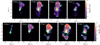 |
Fig. 9 Channel maps of the 2.122 (top panels) and 2.803 µm (bottom panels) H2 lines. Contours are plotted at flux levels of 3, 5, 10, and 30 µJy shown by the cyan lines. |
3.3 The molecular jet and wider angle outflow
As discussed in Harsono et al. (2023), extended molecular hydrogen (H2) emission is detected toward TMC1A with a nearly conical shape that appears to enclose the blueshifted [Fe II] jet. Similar to our analysis of the [Fe II] lines, we investigated the morphology of two of the bright H2 lines (2.122 and 2.803 µm) in detail. For both lines, the structure of the outflow depends on velocity. To examine the kinematic structure of the H2 emission, we plotted flux density maps for each velocity channel with significant H2 emission in Fig. 9. In the highest velocity bins of both 2.122 and 2.803 µm lines, there is evidence for a collimated structure coincident with the axis of the [Fe II] jet. Beyond the jet axis, there is little to no emission at higher velocities (leftmost panel in the top and bottom row of Fig. 9). The line-of-sight velocity for the 2.122 µm H2 line reaches −90 km s−1, and −110 km s−1 for the 2.803 µm, corresponding to −160 km s−1 and −190 km s−1 respectively after de-projection. This lends evidence for a molecular jet component in addition to the atomic jet in TMC1A.
The slower velocity components (∽−30 to +20 km s−1) of the H2 lines make up the wider angle (“shell”) outflow. In comparison to the atomic jet, the width of the H2 outflow is approximately 240 AU at a deprojected distance of 350 AU (2″) from the star while the [Fe II] has a width of ~70 AU at this distance. There is also low-velocity H2 emission present on the redshifted side of the outflow, demonstrating that the H2 outflow is also bipolar, similar to the atomic jet. The southern part of the H2 outflow is also dimmer than the northern part by more than a factor of 10. However, unlike the narrow atomic jet, the redshifted component of the H2 outflow is wider (a width of ~25O AU at 150 AU from star compared to ∽50 AU for the red-shifted [Fe II] outflow at the same distance) and only apparent at lower velocities. The redshifted H2 outflow is also wider than its northern counterpart at the same distance (~250 AU compared to ~ 110 AU at 150 AU from the star).
In the northern H2 outflow, a ring-like structure is observed that exhibits a brightness asymmetry where the right side is 3–4× brighter than the left side (see Fig. 10). The right side includes more redshifted flux compared to the left, which shows little emission at ~60 km s−1 (see Figs. 9 and 10). This may indicate an unresolved velocity gradient associated with the asymmetry.
We further examined the velocity structure using PV diagrams of the 2.803 µm line taken perpendicular to the jet/outflow axis. As with [Fe II], in Fig. 8 (bottom row), solid white dots mark the velocity at peak line emission, which are observed at approximately −30 km s−1 and 20 km s−1 for the blueshifted and redshifted components, respectively. In the first and third columns of the PV diagrams for H2, a transition in peak velocity from −30 km s−1 to 20 km s−1 is observed at the location of the brightness asymmetry in the ring of the H2 shell. However, this shift is not discernible at an intermediate location (the second column) due to marginal differences in the peak flux density between the blueshifted and redshifted velocity bins. Nonetheless, the intensity of the PV diagram still shows an increasing flux density toward the first redshifted velocity bin at this location.
To provide more detailed insights, we plotted the ID spectra at individual spaxels for the 2.803 µm H2 line in the right panel of Fig. 10. The left-side (cyan) of the outflow covers ~3 spectral channels (−70 to +20 km s−1) with the peak emission observed at ∽−30 km s−1. This is in contrast to the right side of the outflow which covers ~4 channels (−70 to +60 km s−1) and peaks at ~20 km s−1 (light red). However, in the southern outflow, the emission includes ~3 spectral channels which lean toward more redshifted velocities (∽−30 to +60 km s−1) (dark red), presumably because the spectra at this location traces the redshifted outflow. Toward the central axis of the northern outflow (dark blue), the line appears broader (~5 channels wide) and shows emission at a notably higher blueshifted velocity, approximately −110 km s−1, corresponding to the jet.
Using the same method as for the [Fe II] 1.644 µm line, peaks in the flux density of the H2 jet were determined by constructing a normalized flux density profile along the jet’s axis at the highest velocity emission (−110 km s−1) of the 2.803 µm line and normalized by the continuum (right panel, Fig. 7). We find that there are similarly three peaks (1H, 2H, 3H) in the blueshifted H2 jet. However, each peak is located at a farther distance from the protostar with respect to the observed [Fe II] peaks (see Sect. 3.2). With a deprojected velocity of ∽−190 km s−1, the three identified peaks in the molecular jet are located at de-projected distances of 245, 350, and 410 AU, corresponding to dynamical timescales of 6, 9, and 10 yr. Notably, the locations of the H2 peaks are found in the brightness dips of the atomic jet (left panel, Fig. 7) suggesting they are situated in between the [Fe II] peaks, although higher spatial resolution observations are needed for confirmation.
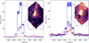 |
Fig. 10 Line profiles of the 1.644 µm [Fe II] (left) and 2.803 µm H2 (right) lines at different locations. The spectra are color-coded and correspond to the locations marked by cross (×) in the moment-0 maps shown in the insets. The spectra are extracted in different locations for the [Fe II] and H2 lines to highlight particular characteristics. In the left panel, these correspond to the three brightness peaks along the blueshiſted jet axis (blue, steel blue, purple) and redshifted jet (red). In the right panel, the spectra correspond to the central spine with higher velocity emission detected (purple), the left (steel blue) and right (blue) wings of the ring-like structure, and the redshiſted outflow (red). |
3.4 Extinction of the jet
The extinction of radiation is a fundamental measure representing the absorption and scattering of light by foreground dust, causing a reddening effect. Accurate determination of the extinction toward the jet is crucial to knowing the actual brightness of several lines used for constraining physical conditions, such as excitation temperatures and densities. We estimated the extinction toward the jet using the observed [Fe II] ratios. The intensity ratio of optically thin lines of the same atom that originate from the same upper level does not depend on the temperature or density of the emitting gas, but rather the ratio of their Einstein A-coefficients via I1/I2 = A1v1/(A2ν2) (Gredel 1994; Giannini et al. 2015; Erkal et al. 2021), where ν1 and ν2 are the frequencies of the two lines. A difference between an observed line ratio value and the intrinsic ratio can therefore be attributed to line-of-sight extinction. Since we detect several transitions of [Fe II] in the jet of TMC1A, we use them to probe extinction. The observations of TMC1A are sufficiently good that we can estimate the extinction of the jet using four separate line ratio pairs.We adopted a similar methodology to Erkal et al. (2021) for determining the extinction of the jet by comparing observed line ratios to the intrinsic ratios tabulated in Giannini et al. (2015), and then using the parameterized extinction curve from Cardelli et al. (1989) to determine the visual extinction, AV, in magnitudes.
We used Eq. (21.1) of Draine (2011), which describes how the extinction at a given wavelength, Aλ, reduces the observed flux  , where Fint is the intrinsic flux and βλ = Aλ/AV. The β terms were determined using the extinction curve from Cardelli et al. (1989), which demonstrated that extinction can be determined solely based on the parameter RV that describes the slope of the extinction at visible wavelengths. We adopted RV = 5.5 as in McClure (2019). Given the well-established intrinsic flux ratios for certain [ion-FeII] lines (Giannini et al. 2015), it is useful to take the ratio of the previous equation at two of these specific wavelengths to then solve for AV (Giannini et al. 2015):
 (1)
(1)
Here  and
and  represent the ratio of A(λ)/A(V) calculated from the extinction curve of Cardelli et al. (1989) (their Eq. (1)). To estimate the uncertainty in the extintion, we propagated uncertainties in the standard way for the intrinsic ratio
  using the standard deviations reported in Giannini et al. (2015), and the observed peak flux
  .
.
Due to the lines spanning only 3–5 velocity bins, we determined the ratio of observed intensities by taking the ratio of the maximum flux densities of each line along the jet’s axis at several different locations/spaxels. The intrinsic ratios of the 1.257/1.644, 1.321/1.644, 1.533/1.677, and 1.599/1.712 µm pairs used in this study were taken from Giannini et al. (2015), and were taken to be 1.1, 0.32, 1.25, and 3.6, respectively. However, the intrinsic line ratio can vary as a result of how the transition probabilities are calculated. For example, the 1.257/1.644 ratio can vary between 0.98 and 1.49 (Rodríguez-Ardila et al. 2004; Smith & Hartigan 2006; Giannini et al. 2015) and more recently an even higher value of 2.6 has been proposed (Rubinstein 2021). For the same observed flux ratio, a difference in the intrinsic ratio of 0.98 to 1.49 corresponds to a difference in AV of ~4 magnitudes while 0.98 to 2.6 increases the difference to ~9. In TMC1A, the observed line ratios for the 1.257/1.644 µm pair range from 0.06–0.2 (values are lower near the protostar). This gives AV of 14–26 (higher AV near the protostar) for an intrinsic ratio of 0.98 and 23–35 for an intrinsic ratio of 2.6. This uncertainty in the intrinsic line ratio results in a substantial uncertainty in the inferred extinction values.
In Fig. 11, we plotted the derived extinction as a function of the de-projected distance along the jet’s axis. The range of AV values span from 10 to 30 magnitudes with uncertainties of approximately ±2–3. Only spaxels with S /N > 3 are shown. We find significant discrepancies in our derived values of extinction when using the less bright [Fe II] line ratios (i.e., 1.533/1.677 and 1.599/1.712). The reason for this discrepancy remains unclear. Nevertheless, across all four line ratio pairs, larger extinction measurements are consistently observed closer to the protostar, gradually decreasing as we move along the jet axis. These findings align with those of Connelley & Greene (2010) for TMC1A (IRAS 04365+2535), where a continuum extinction of  was reported.
We adopted the same analysis for the dimmer southern (red-shifted) jet. Despite that the needed [Fe II] lines are only detected in a few spaxels in the 1.257 µm line, we can estimate the extinction toward the redshifted jet. For two of the brightest spaxels showing emission at 1.257 µm and 1.644 µm, the extinction of the redshifted jet is estimated to be AV ~ 13.8 ± 2.5 through the 1.257/1.644 ratio (F1.257/F1.644=0.24) at the brightest spaxel of the redshifted side and AV ~ 17.4 ± 2.5 for the next brightest spaxel (F1.257/F1.644=0.17). Both redshifted spaxels are located at a de-projected distance of approximately 200 AU from the protostar. At the same distance in the blueshifted jet, the flux ratio is F1.257/F1.644 = 0.09–0.12 corresponding to AV = 21–23 Therefore, the extinction we measure for the redshifted side is comparable to, or even slightly less, than the blueshifted jet, despite having a much lower flux density.
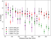 |
Fig. 11 Visual extinction (AV) toward the jet determined from the observed [Fe II] line ratios with respect to their intrinsic ratios. We calculate the line ratios at peak line flux for spaxels along the northern (blueshifted) jet axis. We use the ratio at peak line flux since the lines are only marginally resolved in wavelength (3 or 4 channels). The observed trends are consistent with the values derived from taking line ratios with zeroth-moment maps which have higher uncertainty due to spaxels that contain faint emission. Vertical dashed lines correspond to the three iron peaks in Fig. 7. |
4 Discussion
4.1 Asymmetries in the bipolar outflows
For the first time, we find clear evidence of a redshifted atomic [Fe II] jet in TMC1A moving at a deprojected velocity of ~330 km s−1 to the south of the protostar. In contrast, most of the emission of the blueshifted atomic jet peaks at a deprojected velocity of ~ 120 km s−1, but has emission detected at ~−260 km s−1. The detection of both blue- and redshifted jets indicates the presence of an embedded bipolar jet. In addition, the southern, redshifted, component of the H2 outflow is also revealed. The southern outflow in both the [Fe II] jet and the H2 outflow is 10–30× fainter than the northern counterpart (see Fig. 10). Additionally, the H2 outflow exhibits a brightness asymmetry about the axis of the jet in a ring-like emission feature, where one side of the ring is 3–4× brighter than the other. Below, we address the observed asymmetries and their implications.
4.1.1 Northern and southern outflows
Given the observed intensity and velocity differences in the bipolar outflow components, it is important to determine whether these differences are intrinsic (e.g., in the strength or power of the outflows which we relate to the brightness) or due to external factors such as a nonuniform ambient medium. In the case of TMC1A, our results suggest that differential extinction (from one side of the bipolar outflow to the other) is not the cause of the observed intensity differences: the extinction found in the blueshifted component of the bipolar jet is comparable to the redshifted component (see Sect. 3.4). If the asymmetry was caused by differential extinction, a brightness difference of l0-30× would mean the southern outflow would have a higher extinction on the order of ∆Aλ = 2–4 magnitudes. Assuming this difference in extinction is the same for H2, then the same argument would apply since it is also 10–30× fainter in the south. However, the extinction measured in the southern outflow using the [Fe II] lines is comparable, if not slightly less than the northern outflow. This conclusion is independent of the uncertainties in the intrinsic line ratios, because the observed ratio of the 1.257 µm and 1.644 µm lines in the southern (redshifted) jet is comparable to, or somewhat higher than, the corresponding location in the northern (blueshifted) jet.
A more extincted northern outflow could be caused by a nonuniform line-of-sight gas and dust distribution. Further evidence of the bipolar asymmetry can be seen in the submillimeter CO J = 2–1 (230.5 GHz) emission, which shows the pronounced blue-red side asymmetry, especially in the highest velocity bin (beyond 9 km s−1 from the line center, see Fig. 13 of Aso et al. 2021). The highly collimated CO outflow is essentially one-sided with only the blueshifted component, which is less affected by dust extinction in the submillimeter compared to the infrared. Additional evidence of the asymmetry can be found in other shock tracers such [O I] at 63.2 µm, and OH at 84.6 µm, where detected emission was only found toward the north of the protostar (Karska et al. 2013). The similar asymmetric trend is also seen in TMC1A in 12CO J = 14–13 (Karska et al. 2013), 13CO J = 6–5, J = 3–2 emission (Yıldız et al. 2015) and HCO+ 4–3 emission in the Leiden Observatory Single-dish Sub-mm Spectral Database of Low-mass YSOs (LOMASS) (Carney et al. 2016).
At lower velocities (≲9 km s−1), the northern and southern molecular outflow appears nearly symmetric (Aso et al. 2015, 2021). Furthermore, the large-scale protostellar envelope dust emission around TMC1A, as observed at 450 and 850 µm with the James Clerk Maxwell Telescope’s (JCMT) Submil-limetre Common-User Bolometer Array camera (SCUBA) (Di Francesco et al. 2008), shows no evidence of such asymmetry, other than diffuse emission to the north of TMC1A that may be associated with the surrounding molecular cloud. The lack of asymmetries at slower velocities (i.e. closer to systemic), and a largely symmetric dusty envelope further supports that the asymmetry observed in the [Fe II] jet and H2 emission between the northern and southern sides is the result of an intrinsic difference rather than differential extinction, for example.
In TMC1A, the spatially resolved blue-red asymmetry in the otherwise heavily extincted [Fe II] and H2 outflows can be resolved thanks to the unrivaled sensitivity of the instrument. Follow-up JWST observations that map both sides of the outflow at larger distances from the protostar, beyond the FOV of our observations, and where extinction should be less, would be invaluable in confirming these results. Furthermore, a larger JWST survey of outflows toward more embedded pro-tostars (Class 0-I) in different environmental conditions (e.g., inclination, extinction) will shed light on how common bipolar asymmetries are in younger sources. Indeed, blue-red side asymmetries have been observed in a growing number of older Class II sources (e.g. Woitas et al. 2002; Melnikov et al. 2023). Our observations of TMC1A indicate that this asymmetry can already be present in the younger Class I phase.
4.1.2 The ring-like structure in the H2 outflow
In many of the H2 detections presented, the molecular outflow exhibits a ring-like structure on the northern side, displaying a clear brightness asymmetry about the jet axis. The right side of this ring is 3–4 times brighter than the left side (see Fig. 10). Moreover, this left-right asymmetry is evident in the velocity distribution (Fig. 9), where the right side is more redshifted than the left side, indicating a large-scale velocity gradient from one side of the ring to the other. This trend is further supported in the PV diagrams (see Fig. 8) where the velocity at peak intensity is more redshifted in the region corresponding to the right side of the ring-like structure (−25 km s−1 on left to ~+20 km s−1 on right). The observed structure resembles the partial ring-like structure observed close to the protoplanetary disk of TMC1A in SO NJ = 56 − 45 in Harsono et al. (2021), with a stronger and more redshifted right side compared to the left. Intriguingly, the right side being more redshifted than the left has the same directional sense as the rotation of the protoplanetary disk and CO molecular outflow in TMC1A (Aso et al. 2015, 2021; Bjerkeli et al. 2016; Harsono et al. 2021). That said, the H2 is likely interacting with an asymmetric surrounding medium, which could produce the observed left-right asymmetry in both brightness and line-of-sight velocity (e.g. De Colle et al. 2016).
A better understanding of the left-right asymmetry may come from a comparison of the observed H2 ring-like structure to other molecular lines. Harsono et al. (2021) suggested that the SO emission originates from the warm and dense inner envelope close to the outflow cavity wall. At scales of a few tens of au, both submillimeter HCN J = 3−2 and HCO+ J = 3−2 emission also exhibit similar left-right asymmetry as SO and H2. On larger scales (±~5–10″), the submillimeter C18O J = 2−1 emission traces the flattened envelope, and shows an elongated redshifted component toward the northwest (see Fig. 4 of Aso et al. 2015) which may be associated with the infalling envelope. As mentioned in Sect. 4.1.1, the large-scale dusty envelope also shows a diffuse sub-mm emission along the same direction as the C18O emission at scales greater than 10″(≳1400 AU) from the protostar. This connection may potentially point to a “feeding arm” that is actively adding mass from the molecular cloud to the protostar and preferentially interacting with the northern outflow, but more so where the H2 is brighter. In this scenario, the interaction between the outflow and the nonuniform ambient medium gives rise to the left-right asymmetry.
Finally, it is worth pointing out that the H I and He I emission (see Harsono et al. 2023) is brighter on the left side (opposite of the bright H2 emission on the right side). The emission in both of these atomic lines is dominated by the scattered emission from the unresolved central protostar. The left-right brightness asymmetry could therefore simply arise from radiative transfer effects where scattering dominates the left side of the observed structure where the line-of-sight could go through the outflow cavity while the right side is the line of sight through the edge of the outflow cone providing higher column of gas and dust.
4.2 Atomic and molecular jets in the Class I stage
TMC1A is classified as a Class I protostellar source. It is in an intermediate stage between Class 0 and II sources, possessing both a protostar and disk system while still surrounded by a substantial infalling circumstellar envelope (Lada 1987; Hogerheijde et al. 1998). The atomic jet is traced by [Fe II], while a wider angle molecular “shell” outflow is traced by H2. However, along the spine of the atomic jet, we find tentative evidence of collimated high-velocity, blueshifted (≳ 100 km s−1) H2 emission (see Figs. 9 and 10). The wider molecular “shell” outflow meanwhile has a speed of <70 km s−1. These results suggest that co-spatial molecular and atomic jets are present in TMC1A, and, to the best of our knowledge, this is the first detection of a molecular jet in this source.
In TMC1A, the atomic jet remains significantly brighter and faster (by ~50 km s−1) than its molecular jet counterpart. This would suggest that TMC1A is in the tail end of the transition from a collimated jet that is composed mostly of molecular gas (Class 0 sources) to being mainly atomic (as in Class II sources) (see, e.g., Panoglou et al. 2012; Rabenanahary et al. 2022). This could be because the protostellar envelope and/or a large enough column of dust and gas in the outflow shielding the H2 jet from UV photo-dissociation or that the jet is fast enough to destroy most, but not all, of the H2 through shocks (Tabone et al. 2020). To better understand such differences, deep maps of the atomic and molecular outflow in the near- and mid-IR for a large sample of protostars in different evolutionary stages are essential to better understand how the physical and chemical structure evolves with age.
4.3 Intensity variations in the [Fe II] and H2 jets
Intensity variations and knot-like features have been seen in several protostellar outflows (e.g. Hartigan et al. 2011). In our observations, we observe three distinct flux density peaks in both the blueshifted atomic and molecular jets. Interestingly, we find that the [Fe II] peaks are not quite co-spatial with the H2 peaks: The [Fe II] line peaks at de-projected distances of 200, 270, and 370 AU while the H2 line peaks at de-projected distances of 245, 350, and 410 AU. It appears that the slower (~ 110 km s−1 or 190 km s−1 de-projected) H2 peaks are situated in between the faster (~150 km s−1 or 260 km s−1 de-projected) [Fe II] peaks. While the intensity variations in TMC1A are not spatially well-resolved, they are similar to the knot-like features in some protostellar jets (e.g. Ray et al. 2023; Toledano-Juárez et al. 2023) that are sometimes associated with Herbig-Haro (HH) objects, although historically at much larger (~ tenth of a parsec) scales Reipurth & Bally (2001).
The velocity differences between the H2 and [Fe II] peaks indicate that these features could be produced by a faster atomic jet plowing into a slower molecular outflow. This could explain why the slower (~100 km s−1) peaks in H2 are observed to be in between the faster moving (~150 kms−1) peaks in [Fe II]. In this scenario, molecular material gets excited by shocks in the atomic [Fe II] jet, which then cool, resulting in the H2 emission peaking in these regions.
The observed peaks may also be attributed to episodic mass ejection events (e.g. Bonito et al. 2010) where the formation of chains of knots could be due to a variable mass-ejection rate from the protostar and disk (e.g. Arce et al. 2007), which is closely linked to episodic accretion onto the protostar (e.g. Plunkett et al. 2015; Vorobyov et al. 2018). The intensity variations observed in TMC1A resemble the knots observed in other “microjets” such as in DG Tau, where knots are inferred to form on timescales of just a few years (Agra-Amboage et al. 2011) or 10–15 yr in the case of TH 28 (Murphy et al. 2021). In the episodic mass ejection scenario, the H2 emission peaks appearing in the valleys of the [Fe II] emission in TMC1A would correspond to periods in between ejection events. In either case, higher spatial and spectral resolution observations, and/or several epochs of observations, will be necessary to confirm such a scenario.
Since the dynamical timescales associated with each successive observed peak along the jet axis are relatively small (<10 yr), periodically observing the outflow could reveal not only the movement of the detected intensity peaks, but also the formation of any new peaks in both [Fe II] and H2. This would inform us about the interaction and evolution of the atomic and molecular knot-like structures. With JWST in particular, the simultaneous monitoring of near-IR atomic H recombination lines (such as Hβ at 1.282 µm and Hα at 4.052 µm) would reveal changes in the protostellar accretion rate and its relation to the evolution and possible creation of new knot-like structures. This would further our understanding of the dynamic processes driving the redistribution of material in protostellar systems as a function of time.
5 Conclusions
We analyze near-IR JWST observations of [Fe II] and H2 lines detected toward the Class I protostar, TMC1A, to study the structure of its protostellar outflows. The spectra of the TMC1A outflow show numerous [Fe II] and H2 lines. In total, we detect 30 [Fe II] lines and 26 H2 lines in our NIRSpec IFU observations with the G140H, G235H and G395H gratings (see Figs. 2–5). Our findings can be summarized as follows:
The observed [Fe II] 1.644 µm emission peaks at around −70 km s−1 and reach velocities upward of −150 km s−1, corresponding to approximately −120 and −260 km s−1 after de-projection. For the first time, the redshifted counterpart of the atomic jet is seen, which is only detected in the bright 1.644 and 1.810 µm [Fe II] lines. The southern redshifted emission is significantly dimmer (by a factor 10-30×) and faster than the blueshifted component (peaking at ~190 km s−1 with tentative emission at 230 km s−1 or ~330 and ~400 km s−1 after de-projection). The atomic jet in TMC1A is bipolar;
We find tentative evidence of a fast collimated H2 outflow with emission above 3-σ at radial velocities of ~110 km s−1 (~190 km s−1 deprojected) on the blueshifted side of the outflow. It indicates that the jet toward TMC1A is also molecular in addition to the wider angle (slower) H2 shell;
Similar to [Fe II] emission, H2 emission is also detected in the southern part of the protostar indicating that it is also bipolar and tends to be more redshifted than the northern outflow. The H2 outflow is 2–4× wider in both the northern and southern outflows than the atomic [Fe II] jet and the southern side is > 2× wider than the northern counterpart at the same deprojected distance;
Both [Fe II] and H2 high-velocity emission (υ ~ 100150 km s−1) show three distinct peaks that are not co-spatial. From the deprojected velocities and distances, [Fe II] emissions peak at 200, 270, and 370 AU. On the other hand, H2 emission peaks at 245, 350, 410 AU. Furthermore, at the peak locations, H2 is observed to be slower than the closest [Fe II] emission;
With the detected [Fe II] lines, we derive a range of visual extinction from AV = 10–30 that decreases with distance from the central protostar for the northern blueshifted part. For the redshifted jet, a comparable extinction is derived from 1.257/1.644 µm line ratio pair;
The large difference in [Fe II] line flux and velocity between the redshifted and blueshifted jet components may indicate that the red-blue asymmetry commonly observed in more evolved Class II jets can already start in the earlier Class I phase. We showed the blue-red brightness asymmetry is not due to differential extinction, but is rather an intrinsic brightness difference;
The collimated atomic and molecular jet in TMC1A illustrates a scenario in which molecular jets, typical in Class 0 stages, and atomic jets, prevalent in Class II stages where molecular outflows are observed at wider angles, coexist in the intermediate Class I stage. The presence of a brighter and faster atomic jet compared to the molecular jet, including the slower, wider-angle molecular shell, suggests that TMC1A may be near the tail end of this transitional phase of outflows;
The peaks in flux profiles within the atomic and molecular jet resemble Herbig-Haro object knots but at smaller scales (a few hundred AU vs. parsecs), with the slower molecular peaks and offset disparities suggesting the possibility of the atomic jet driving the molecular jet. Their dynamical timescales, less than 10 years and with only a few years’ difference, imply recent or ongoing outbursts.
The observations of TMC1A presented here are a great example of the NIRSpec IFU’s ability to detect a wealth of [Fe II] and H2 lines in the near-IR, even in the case of the highly extincted environments of protostars and, in the case of TMC1A, revealing high-velocity outflow components and brightness asymmetries. In future work, we will examine the range of excitation conditions that can be constrained by the large number of forbidden iron lines and H2 lines detected here, which will permit us to better characterize the physical conditions of the outflow and its respective mass outflow rates.
Acknowledgements
This work was supported in part by an ALMA SOS award, STScI JWST-GO-02104.002-A, NSF grant AST-1910106 and NASA ATP grant 80NSSC20K0533. This work is based on observations made with the NASA/ESA/CSA James Webb Space Telescope. The data were obtained from the Mikulski Archive for Space Telescopes at the Space Telescope Science Institute, which is operated by the Association of Universities for Research in Astronomy, Inc., under NASA contract NAS 5-03127 for JWST. These observations are associated with GO program #2104. DH is supported by a Center for Informatics and Computation in Astronomy (CICA) grant and grant number 110J0353I9 from the Ministry of Education of Taiwan. DH also acknowledges support from the National Science and Technology Council of Taiwan through grant number 111B3005191. LT acknowledges support from the Netherlands Research School for Astronomy (NOVA). A portion of this research was carried out at the Jet Propulsion Laboratory, California Institute of Technology, under a contract with the National Aeronautics and Space Administration (80NM0018D0004). We thank the referee for a constructive and timely report that helped improve the paper.
Appendix A Detected lines
The list of detected lines for both [Fe II] and H2 are reported in Table A.1 with observational details and the properties of each line taken from the Atomic Line List version:3.00b5 and NIST Atomic Spectra Database for [Fe II] and the Gemini Important H2 lines list for H2. We report the intensity line ratios with respect to prominent lines (1.644 for [Fe II] and 2.122 for H2)
[Fe II] and H2 detections
References
- Agra-Amboage, V., Dougados, C., Cabrit, S., & Reunanen, J. 2011, A&A, 532, A59 [NASA ADS] [CrossRef] [EDP Sciences] [Google Scholar]
- Agra-Amboage, V., Cabrit, S., Dougados, C., et al. 2014, A&A, 564, A11 [NASA ADS] [CrossRef] [EDP Sciences] [Google Scholar]
- Arce, H. G., Shepherd, D., Gueth, F., et al. 2007, in Protostars and Planets V, eds. B. Reipurth, D. Jewitt, & K. Keil, 245 [Google Scholar]
- Aso, Y., Ohashi, N., Saigo, K., et al. 2015, ApJ, 812, 27 [Google Scholar]
- Aso, Y., Kwon, W., Hirano, N., et al. 2021, ApJ, 920, 71 [NASA ADS] [CrossRef] [Google Scholar]
- Bally, J. 2016, ARA&A, 54, 491 [Google Scholar]
- Bally, J., Reipurth, B., & Davis, C. J. 2007, in Protostars and Planets V, eds. B. Reipurth, D. Jewitt, & K. Keil, 215 [Google Scholar]
- Beck, T. L., McGregor, P. J., Takami, M., & Pyo, T.-S. 2008, ApJ, 676, 472 [NASA ADS] [CrossRef] [Google Scholar]
- Beuther, H., van Dishoeck, E. F., Tychoniec, L., et al. 2023, A&A, 673, A121 [NASA ADS] [CrossRef] [EDP Sciences] [Google Scholar]
- Bjerkeli, P., van der Wiel, M. H. D., Harsono, D., Ramsey, J. P., & Jørgensen, J. K. 2016, Nature, 540, 406 [Google Scholar]
- Böker, T., Arribas, S., Lützgendorf, N., et al. 2022, A&A, 661, A82 [NASA ADS] [CrossRef] [EDP Sciences] [Google Scholar]
- Böker, T., Beck, T., Birkmann, S., et al. 2023, PASP, 135, 038001 [CrossRef] [Google Scholar]
- Bonito, R., Orlando, S., Peres, G., et al. 2010, A&A, 511, A42 [NASA ADS] [CrossRef] [EDP Sciences] [Google Scholar]
- Bontemps, S., Andre, P., Terebey, S., & Cabrit, S. 1996, A&A, 311, 858 [NASA ADS] [Google Scholar]
- Bushouse, H., Eisenhamer, J., Dencheva, N., et al. 2023a, https://doi.org/10.5281/zenodo.7714020 [Google Scholar]
- Bushouse, H., Eisenhamer, J., Dencheva, N., et al. 2023b, https://doi.org/10.5281/zenodo.8247246 [Google Scholar]
- Cabrit, S., Ferreira, J., & Dougados, C. 2011, in IAU Symp., 275, eds. G. E. Romero, R. A. Sunyaev, & T. Belloni, 374 [NASA ADS] [Google Scholar]
- Cardelli, J. A., Clayton, G. C., & Mathis, J. S. 1989, ApJ, 345, 245 [Google Scholar]
- Carney, M. T., Yildiz, U. A., Mottram, J. C., et al. 2016, A&A, 586, A44 [NASA ADS] [CrossRef] [EDP Sciences] [Google Scholar]
- Cernicharo, J., & Reipurth, B. 1996, ApJ, 460, L57 [NASA ADS] [CrossRef] [Google Scholar]
- Chandler, C. J., Terebey, S., Barsony, M., Moore, T. J. T., & Gautier, T. N. 1996, ApJ, 471, 308 [NASA ADS] [CrossRef] [Google Scholar]
- Connelley, M. S., & Greene, T. P. 2010, AJ, 140, 1214 [Google Scholar]
- Dabrowski, I. 1984, Can. J. Phys., 62, 1639 [NASA ADS] [CrossRef] [Google Scholar]
- Davis, C. J., Whelan, E., Ray, T. P., & Chrysostomou, A. 2003, A&A, 397, 693 [CrossRef] [EDP Sciences] [Google Scholar]
- De Colle, F., Cerqueira, A. H., & Riera, A. 2016, ApJ, 832, 152 [NASA ADS] [CrossRef] [Google Scholar]
- Delabrosse, V., Dougados, C., Cabrit, S., et al. 2024, A&A in press, https://www.doi.org/10.1051/0004-6361/202449176 [Google Scholar]
- De Valon, A., Dougados, C., Cabrit, S., et al. 2020, A&A, 634, A12 [Google Scholar]
- Di Francesco, J., Johnstone, D., Kirk, H., MacKenzie, T., & Ledwosinska, E. 2008, ApJS, 175, 277 [Google Scholar]
- Dionatos, O., Nisini, B., Garcia Lopez, R., et al. 2009, ApJ, 692, 1 [NASA ADS] [CrossRef] [Google Scholar]
- Dionatos, O., Nisini, B., Cabrit, S., Kristensen, L., & Pineau Des Forêts, G. 2010, A&A, 521, A7 [NASA ADS] [CrossRef] [EDP Sciences] [Google Scholar]
- Draine, B. T. 2011, Physics of the Interstellar and Intergalactic Medium (Princeton University Press) [Google Scholar]
- Erkal, J., Nisini, B., Coffey, D., et al. 2021, ApJ, 919, 23 [NASA ADS] [CrossRef] [Google Scholar]
- Federman, S. A., Megeath, S. T., Rubinstein, A. E., et al. 2024, ApJ, 966, 41 [CrossRef] [Google Scholar]
- Fedriani, R., Caratti o Garatti, A., Purser, S. J. D., et al. 2019, Nat. Commun., 10, 3630 [NASA ADS] [CrossRef] [Google Scholar]
- Frank, A. 1999, New Astron. Rev., 43, 31 [CrossRef] [Google Scholar]
- Frank, A., Ray, T. P., Cabrit, S., et al. 2014, Protostars and Planets VI, eds. H. Beuther, R. S. Klessen, C. P. Dullemond, & T. Henning, 451 [Google Scholar]
- Galli, P., Loinard, L., Bouy, H., et al. 2019, A&A, 630, A137 [NASA ADS] [CrossRef] [EDP Sciences] [Google Scholar]
- Giannini, T., Calzoletti, L., Nisini, B., et al. 2008, A&A, 481, 123 [NASA ADS] [CrossRef] [EDP Sciences] [Google Scholar]
- Giannini, T., Nisini, B., Antoniucci, S., et al. 2013, ApJ, 778, 71 [NASA ADS] [CrossRef] [Google Scholar]
- Giannini, T., Antoniucci, S., Nisini, B., et al. 2015, ApJ, 798, 33 [Google Scholar]
- Godard, B., Pineau des Forêts, G., Lesaffre, P., et al. 2019, A&A, 622, A100 [NASA ADS] [CrossRef] [EDP Sciences] [Google Scholar]
- Gredel, R. 1994, A&A, 292, 580 [NASA ADS] [Google Scholar]
- Greenfield, P., & Miller, T. 2016, Astron. Comput., 16, 41 [NASA ADS] [Google Scholar]
- Haro, G. 1952, ApJ, 115, 572 [NASA ADS] [CrossRef] [Google Scholar]
- Harsono, D., van der Wiel, M., Bjerkeli, P., et al. 2021, A&A, 646, A72 [NASA ADS] [CrossRef] [EDP Sciences] [Google Scholar]
- Harsono, D., Bjerkeli, P., Ramsey, J. P., et al. 2023, ApJ, 951, L32 [NASA ADS] [CrossRef] [Google Scholar]
- Hartigan, P., Edwards, S., & Ghandour, L. 1995, ApJ, 452, 736 [Google Scholar]
- Hartigan, P., Frank, A., Foster, J. M., et al. 2011, ApJ, 736, 29 [Google Scholar]
- Herbig, G. H. 1951, ApJ, 113, 697 [NASA ADS] [CrossRef] [Google Scholar]
- Hirth, G. A., Mundt, R., & Solf, J. 1997, A&AS, 126, 437 [NASA ADS] [CrossRef] [EDP Sciences] [Google Scholar]
- Hogerheijde, M. R., van Dishoeck, E. F., Blake, G. A., & van Langevelde, H. J. 1998, ApJ, 502, 315 [NASA ADS] [CrossRef] [Google Scholar]
- Jakobsen, P., Ferruit, P., de Oliveira, C. A., et al. 2022, A&A, 661, A80 [NASA ADS] [CrossRef] [EDP Sciences] [Google Scholar]
- Karska, A., Herczeg, G. J., van Dishoeck, E. F., et al. 2013, A&A, 552, A141 [NASA ADS] [CrossRef] [EDP Sciences] [Google Scholar]
- Koo, B.-C., Raymond, J. C., & Kim, H.-J. 2016, J. Korean Astron. Soc., 49, 109 [NASA ADS] [CrossRef] [Google Scholar]
- Kramida, A., Yu. Ralchenko, Reader, J., & NIST ASD Team 2023, NIST Atomic Spectra Database (ver. 5.11), https://physics.nist.gov/asd (National Institute of Standards and Technology, Gaithersburg, MD) [Google Scholar]
- Lada, C. J. 1987, in Star Forming Regions, 115, eds. M. Peimbert, & J. Jugaku, 1 [NASA ADS] [Google Scholar]
- Lee, C.-F., Li, Z.-Y., Hirano, N., et al. 2018, ApJ, 863, 94 [NASA ADS] [CrossRef] [Google Scholar]
- Liu, C.-F., Shang, H., Pyo, T.-S., et al. 2012, ApJ, 749, 62 [NASA ADS] [CrossRef] [Google Scholar]
- McClure, M. 2019, A&A, 632, A32 [NASA ADS] [CrossRef] [EDP Sciences] [Google Scholar]
- Melnick, G. J., & Kaufman, M. J. 2015, ApJ, 806, 227 [NASA ADS] [CrossRef] [Google Scholar]
- Melnikov, S., Boley, P. A., Nikonova, N. S., et al. 2023, A&A, 673, A156 [NASA ADS] [CrossRef] [EDP Sciences] [Google Scholar]
- Mundt, R., & Fried, J. W. 1983, ApJ, 274, L83 [NASA ADS] [CrossRef] [Google Scholar]
- Mundt, R., Buehrke, T., Solf, J., Ray, T. P., & Raga, A. C. 1990, A&A, 232, 37 [Google Scholar]
- Murphy, A., Dougados, C., Whelan, E. T., et al. 2021, A&A, 652, A119 [NASA ADS] [CrossRef] [EDP Sciences] [Google Scholar]
- Myers, P. C., Dunham, M. M., & Stephens, I. W. 2023, ApJ, 949, 19 [NASA ADS] [CrossRef] [Google Scholar]
- Narang, M., Manoj, P., Tyagi, H., et al. 2024, ApJ, 962, L16 [NASA ADS] [CrossRef] [Google Scholar]
- Nisini, B., Bacciotti, F., Giannini, T., et al. 2005, A&A, 441, 159 [NASA ADS] [CrossRef] [EDP Sciences] [Google Scholar]
- Nisini, B., Santangelo, G., Giannini, T., et al. 2015, ApJ, 801, 121 [NASA ADS] [CrossRef] [Google Scholar]
- Nisini, B., Navarro, M. G., Giannini, T., et al. 2024, ApJ, 967, 168 [NASA ADS] [CrossRef] [Google Scholar]
- Oliva, E., Marconi, A., Maiolino, R., et al. 2001, A&A, 369, L5 [NASA ADS] [CrossRef] [EDP Sciences] [Google Scholar]
- Panoglou, D., Cabrit, S., Pineau Des Forêts, G., et al. 2012, A&A, 538, A2 [CrossRef] [EDP Sciences] [Google Scholar]
- Pascucci, I., Cabrit, S., Edwards, S., et al. 2023, Protostars and Planets VII, ASP Conf. Ser., eds. S. Inutsuka, Y. Aikawa, T. Muto, K. Tomida, & M. Tamura, 534, 567 [NASA ADS] [Google Scholar]
- Plunkett, A. L., Arce, H. G., Mardones, D., et al. 2015, Nature, 527, 70 [NASA ADS] [CrossRef] [Google Scholar]
- Podio, L., Bacciotti, F., Nisini, B., et al. 2006, A&A, 456, 189 [NASA ADS] [CrossRef] [EDP Sciences] [Google Scholar]
- Podio, L., Eislöffel, J., Melnikov, S., Hodapp, K. W., & Bacciotti, F. 2011, A&A, 527, A13 [NASA ADS] [CrossRef] [EDP Sciences] [Google Scholar]
- Podio, L., Tabone, B., Codella, C., et al. 2021, A&A, 648, A45 [NASA ADS] [CrossRef] [EDP Sciences] [Google Scholar]
- Rabenanahary, M., Cabrit, S., Meliani, Z., & Pineau des Forêts, G. 2022, A&A, 664, A118 [NASA ADS] [CrossRef] [EDP Sciences] [Google Scholar]
- Ray, T. P., Mundt, R., Dyson, J. E., Falle, S. A. E. G., & Raga, A. C. 1996, ApJ, 468, L103 [Google Scholar]
- Ray, T., Dougados, C., Bacciotti, F., Eislöffel, J., & Chrysostomou, A. 2007, in Protostars and Planets V, eds. B. Reipurth, D. Jewitt, & K. Keil, 231 [Google Scholar]
- Ray, T. P., McCaughrean, M. J., Caratti o Garatti, A., et al. 2023, Nature, 622, 48 [NASA ADS] [CrossRef] [Google Scholar]
- Reipurth, B., & Bally, J. 2001, ARA&A, 39, 403 [Google Scholar]
- Reipurth, B., & Heathcote, S. 1997, in IAU Symp., Herbig-Haro Flows and the Birth of Stars, eds. B. Reipurth, & C. Bertout (Springer, Dordrecht), 182, 3 [NASA ADS] [CrossRef] [Google Scholar]
- Reipurth, B., Hartigan, P., Heathcote, S., Morse, J. A., & Bally, J. 1997, AJ, 114, 757 [NASA ADS] [CrossRef] [Google Scholar]
- Reipurth, B., Davis, C. J., Bally, J., et al. 2019, AJ, 158, 107 [NASA ADS] [CrossRef] [Google Scholar]
- Rieke, G. H., Wright, G., Böker, T., et al. 2015, PASP, 127, 584 [NASA ADS] [CrossRef] [Google Scholar]
- Rodríguez-Ardila, A., Pastoriza, M. G., Viegas, S., Sigut, T. A. A., & Pradhan, A. K. 2004, A&A, 425, 457 [NASA ADS] [CrossRef] [EDP Sciences] [Google Scholar]
- Rubinstein, A. E. 2021, RNAAS, 5, 214 [NASA ADS] [Google Scholar]
- Seale, J. P., & Looney, L. W. 2008, ApJ, 675, 427 [NASA ADS] [CrossRef] [Google Scholar]
- Shu, F. H., & Adams, F. C. 1987, in IAU Symp., Cambridge University Press, 122, 7 [Google Scholar]
- Smith, N., & Hartigan, P. 2006, ApJ, 638, 1045 [NASA ADS] [CrossRef] [Google Scholar]
- Sperling, T., Eislöffel, J., Fischer, C., et al. 2021, A&A, 650, A173 [CrossRef] [EDP Sciences] [Google Scholar]
- Sturm, J. A., McClure, M. K., Beck, T. L., et al. 2023, A&A, 679, A138 [NASA ADS] [CrossRef] [EDP Sciences] [Google Scholar]
- Tabone, B., Godard, B., Pineau des Forêts, G., Cabrit, S., & van Dishoeck, E. F. 2020, A&A, 636, A60 [NASA ADS] [CrossRef] [EDP Sciences] [Google Scholar]
- Toledano-Juárez, I., de la Fuente, E., Trinidad, M. A., Tafoya, D., & Nigoche-Netro, A. 2023, MNRAS, 522, 1591 [CrossRef] [Google Scholar]
- Turner, J., Kirby-Docken, K., & Dalgarno, A. 1977, ApJS, 35, 281 [NASA ADS] [CrossRef] [Google Scholar]
- Tychoniec, L., Hull, C. L. H., Kristensen, L. E., et al. 2019, A&A, 632, A101 [NASA ADS] [CrossRef] [EDP Sciences] [Google Scholar]
- Tychoniec, L., van Dishoeck, E. F., van’t Hoff, M. L. R., et al. 2021, A&A, 655, A65 [NASA ADS] [CrossRef] [EDP Sciences] [Google Scholar]
- van Hoof, P. A. M. 2018, Galaxies, 6, 63 [NASA ADS] [CrossRef] [Google Scholar]
- Vorobyov, E. I., Elbakyan, V. G., Plunkett, A. L., et al. 2018, A&A, 613, A18 [NASA ADS] [CrossRef] [EDP Sciences] [Google Scholar]
- White, M. C., Bicknell, G. V., McGregor, P. J., & Salmeron, R. 2014, MNRAS, 442, 28 [Google Scholar]
- Woitas, J., Ray, T. P., Bacciotti, F., Davis, C. J., & Eislöffel, J. 2002, ApJ, 580, 336 [NASA ADS] [CrossRef] [Google Scholar]
- Wright, G., Wright, D., Goodson, G., et al. 2015, PASP, 127, 595 [NASA ADS] [CrossRef] [Google Scholar]
- Yang, Y.-L., Green, J. D., Pontoppidan, K. M., et al. 2022, ApJ, 941, L13 [NASA ADS] [CrossRef] [Google Scholar]
- Yıldız, U. A., Kristensen, L. E., van Dishoeck, E. F., et al. 2015, A&A, 576, A109 [NASA ADS] [CrossRef] [EDP Sciences] [Google Scholar]
- Zapata, L. A., Lizano, S., Rodriguez, L. F., et al. 2015, ApJ, 798, 131 [NASA ADS] [CrossRef] [Google Scholar]
All Tables
All Figures
|
Fig. 1 Illustration of the data reduction process for the 1.644 µm [Fe II] line. (A) Integrated flux density maps (moment 0) of the line after the pipeline. (B) Result of the continuum fit. (C) Continuum-subtracted emission map. (D) Continuum-subtracted map with an S/N cut (Fλ ≥ 3). (E) Zeroth moment map after removal of bad spaxels. |
| In the text | |
|
Fig. 2 Detected [Fe II] emission lines in order of increasing wavelength. Each panel shows a spectrum taken in the northern part of the outflow along the jet axis (~0.5 arcsec away from the protostar). The location of the spaxel is shown as a cross (×) in the panel of the 1.644 µm line of Fig. 3. Meanwhile, the 4.889 µm spectrum is extracted from a location that is marked by the cross in the panel for the 4.889 µm in Fig. 3 to avoid the contamination by the CO fundamental ro-vibrational line. Velocities are calculated independently for each line with respect to the rest wavelength (see Table A.1). The wavelength in microns is given in the upper left of each panel, and the transition terms are given in the upper right and summarized in Table A.1. The 1.749 µm line is blended with the H2 1–0 S(7) line and each is labeled in the inset. Similarly the Br 18 hydrogen recombination line is denoted in the 1.534 µm line. The 1σ uncertainty including a 5% calibration uncertainty is shown by the shaded region. |
| In the text | |
|
Fig. 3 Each panel shows the peak flux density map of the detected [Fe II] lines with an S /N ≥ 3 and bad pixels masked out. The black cross (×) with white borders in the panel for the 1.644 µm line denotes the spaxel used to extract the 1D spectra in Fig. 2. A different spaxel is used to extract the 4.89 µm line profile since it is affected by contamination closer to the protostar. The redshifted or southern part of the outflow discussed in later sections (see Sect. 3.2) does not appear in these maps since we plotted the flux density maps at the velocity corresponding to the peak line flux for a spaxel located in the blueshifted side of the jet. The rest wavelength in microns of each line is overplotted in the upper left of each panel. |
| In the text | |
|
Fig. 4 Line profiles of the detected H2 emission lines in order of increasing wavelength. Each spectrum was taken in the northern part of the outflow marked by the black cross (×) in the 2.122 µm panel of Fig. 5. This location was chosen because this region is bright in H2, while the contamination from scattered light that is worse at longer wavelengths is minimized, easing the detection of weaker line emission. |
| In the text | |
|
Fig. 5 Peak flux density maps of the detected H2 lines similar to Fig. 3. The black cross (×) with white borders in the 2.122 µm panel corresponds to the spaxel where the spectra in Fig. 4 were taken. |
| In the text | |
|
Fig. 6 Channel maps of the 1.644 µm [Fe II] line. Contours are plotted at 1.5, 2.5, 5, and 15 µJy. |
| In the text | |
|
Fig. 7 Peaks in the [Fe II] (left) and H2 (right) outflows. The flux density profile of the highest velocity emission as a function of the deprojected distance along the jet’s axis (−150 km s−1 for [Fe II], −110 km s−1 for H2) is shown normalized with respect to the dust continuum. The inset in each panel shows the flux density maps with color maps logarithmically spaced from 10−2 to 10 µJy. The dashed vertical lines correspond to the peak (central) position of each peak determined by fitting Gaussian profile to the flux density profile (Fline/Fcont vs distance). The same locations are indicated by the white dashed lines in the flux density map in the inset. |
| In the text | |
|
Fig. 8 PV diagrams of the 1.644 µm [Fe II] (top row) and 2.803 µm H2 (bottom row) lines at different locations in the bipolar jet. The distance offset from the jet axis is calculated by adopting a distance of 140 pc without de-projection since the slices are taken perpendicular to the jet. The de-projected offsets are shown in the bottom left of each panel. In each panel, the integrated flux density or moment-0 maps are shown in the inset along with the region that the PV diagram was taken which has a width of 4 spaxels. |
| In the text | |
|
Fig. 9 Channel maps of the 2.122 (top panels) and 2.803 µm (bottom panels) H2 lines. Contours are plotted at flux levels of 3, 5, 10, and 30 µJy shown by the cyan lines. |
| In the text | |
|
Fig. 10 Line profiles of the 1.644 µm [Fe II] (left) and 2.803 µm H2 (right) lines at different locations. The spectra are color-coded and correspond to the locations marked by cross (×) in the moment-0 maps shown in the insets. The spectra are extracted in different locations for the [Fe II] and H2 lines to highlight particular characteristics. In the left panel, these correspond to the three brightness peaks along the blueshiſted jet axis (blue, steel blue, purple) and redshifted jet (red). In the right panel, the spectra correspond to the central spine with higher velocity emission detected (purple), the left (steel blue) and right (blue) wings of the ring-like structure, and the redshiſted outflow (red). |
| In the text | |
|
Fig. 11 Visual extinction (AV) toward the jet determined from the observed [Fe II] line ratios with respect to their intrinsic ratios. We calculate the line ratios at peak line flux for spaxels along the northern (blueshifted) jet axis. We use the ratio at peak line flux since the lines are only marginally resolved in wavelength (3 or 4 channels). The observed trends are consistent with the values derived from taking line ratios with zeroth-moment maps which have higher uncertainty due to spaxels that contain faint emission. Vertical dashed lines correspond to the three iron peaks in Fig. 7. |
| In the text | |
Current usage metrics show cumulative count of Article Views (full-text article views including HTML views, PDF and ePub downloads, according to the available data) and Abstracts Views on Vision4Press platform.
Data correspond to usage on the plateform after 2015. The current usage metrics is available 48-96 hours after online publication and is updated daily on week days.
Initial download of the metrics may take a while.