| Issue |
A&A
Volume 688, August 2024
|
|
|---|---|---|
| Article Number | A173 | |
| Number of page(s) | 22 | |
| Section | Stellar structure and evolution | |
| DOI | https://doi.org/10.1051/0004-6361/202449176 | |
| Published online | 20 August 2024 | |
JWST study of the DG Tau B disk-wind candidate
I. Overview and nested H2-CO outflows
1
Univ. Grenoble-Alpes, CNRS, IPAG, 38000 Grenoble, France
2
Observatoire de Paris, PSL University, Sorbonne University, CNRS, LERMA, 75014 Paris, France
3
Univ. Paris-Saclay, CNRS, Institut d’Astrophysique Spatiale, 91405 Orsay, France
4
Leiden Observatory, Leiden University, PO Box 9513 2300 RA Leiden, The Netherlands
5
School of Cosmic Physics, Dublin Institute for Advanced Studies, Dublin, Ireland
6
INAF, Osservatorio Astrofisico di Arcetri, 50125 Firenze, Italy
Received:
8
January
2024
Accepted:
5
April
2024
Context. The origin of outflows and their impact on protoplanetary disk evolution and planet-formation processes are still crucial open questions. DG Tau B is a Class I protostar associated with a structured disk and a rotating conical CO outflow and was recently identified by ALMA as one of the best CO disk wind candidate. It is therefore a perfect target for studying these questions.
Aims. We aim to map and study any outflow component intermediate between the axial jet and the CO outflow in order to constrain the origin (irradiated or shocked disk wind or swept-up material) of the redshifted molecular outflows in DG Tau B.
Methods. We analyzed observations obtained with James Webb Space Telescope NIRSpec-IFU and NIRCam, supplemented with IFU data from the SINFONI/VLT instrument. We investigated the morphology, kinematics, and excitation conditions of the ro-vibrational H2 emission lines and their relation with the atomic jet and CO outflow. We focus our analysis on the redshifted outflow lobe.
Results. We observe a global layered structure of the redshifted outflows in DG Tau B, with the atomic jet inside the H2 cavity, which in turn is nested inside the CO conical outflow. We also find temperature, velocity, and collimation to be increasing towards the axis of the flow. The redshifted H2 emission traces a narrow conical cavity (semi-opening angle of 9.4°) that is wider than the axial jet but nested just inside the CO outflow. Both the jet and the H2 cavity originate from the innermost regions of the disk (r0 < 6 au). The redshifted H2 cavity flows with a constant vertical velocity of Vz = 22.5 ± 0.8 km s−1, twice faster than the conical CO flow. The excitation conditions imply a hot H2 gas (Tex ≃ 2200 K) with an average mass flux of Ṁ(H2) = 3 × 10⁻¹¹ M⊙ yr−1, which is significantly lower than the jet and CO values.
Conclusions. The global layered H2-CO structure in temperature, velocity, and collimation in the DG Tau B redshifted lobe is consistent with a magneto-hydrodynamic disk wind scenario. The hot H2 could trace the inner, dense photodissociation layer in the wind. An H2 launching region at disk radii of 0.2−0.4 au combined with a large ejection efficiency (ξ ≃ 1) would account for the mass flux and kinematics. Alternatively, the near-IR ro-vibrational H2 could be emitted in the interaction layer driven by successive jet bow shocks into an outer disk wind or envelope. Further constraints on both scenarios will be obtained from the analysis of MIRI observations.
Key words: techniques: imaging spectroscopy / stars: formation / stars: individual: [EM98] DG Tau B cRN / stars: protostars / stars: winds / outflows / infrared: stars
© The Authors 2024
 Open Access article, published by EDP Sciences, under the terms of the Creative Commons Attribution License (https://creativecommons.org/licenses/by/4.0), which permits unrestricted use, distribution, and reproduction in any medium, provided the original work is properly cited.
This article is published in open access under the Subscribe to Open model. Subscribe to A&A to support open access publication.
1. Introduction
Star formation is accompanied by striking and powerful bipolar ejections. Two prominent components are observed: collimated and fast axial jets, and wider low-velocity outflows. These ejection signatures are detectable throughout the star-formation process, from Class 0 onwards and may have a major impact on the final mass of the star and disk accretion process, by potentially carrying a significant fraction of the system mass and angular momentum (see for a recent review Pascucci et al. 2023).
Slow molecular outflows (< 10 km s−1) observed in CO lines are traditionally interpreted as swept-up material, tracing the interaction between the inner jet and/or wide-angle wind and the infalling envelope or parent core. However, recent interferometric observations probing CO outflows from the driving source on smaller scales (less than a few thousand astronomical units (au)) suggest an additional contribution. These observations reveal outflowing conical “cavities” anchored well inside the disk, also detected in more evolved Class II sources with no evidence for a residual envelope (e.g., HH30: Louvet et al. 2018). Rotation signatures consistent with an origin in the inner regions of the disk (r0 ≃ 0.1 − 40 au) have been detected in most cases (Launhardt et al. 2009; Zapata et al. 2015; Bjerkeli et al. 2016; Tabone et al. 2017; Louvet et al. 2018; de Valon et al. 2020, 2022; López-Vázquez et al. 2024). The inferred mass fluxes are very significant, on the order of the mass-accretion rate onto the star, and largely exceed the levels achievable by disk photoevaporation (Pascucci et al. 2023).
These observations suggest that part of the small-scale emission in these slow molecular outflows could trace matter directly ejected from the disk by magnetic processes (e.g., Pudritz et al. 2006; Bai et al. 2016). Such magnetic disk winds, if fully confirmed, would have a crucial impact on the evolution of protoplanetary disk; they would solve the problem of angular momentum transport in the low-ionization dead zones of disks where MRI turbulence is quenched (e.g., Bai et al. 2016; Riols & Lesur 2018) and would significantly affect the disk properties, in particular the surface density profile, affecting planet formation and migration (Kimmig et al. 2020).
However, the swept-up interpretation cannot be fully excluded at this stage. To test this scenario, we are critically missing resolved spatial information on any gas component filling the gap between the fast axial jets and the slow and cold molecular outflows. In the disk-wind paradigm, such a component would trace streamlines with intermediate velocities (a few 10 km s−1) and temperatures (from a few hundred K to a few thousand K), which are expected to emit preferentially in the near and mid-IR domain. With ground-based IFUs, such as SINFONI/VLT and NIFS/Gemini, it is possible to probe the gas component at 2000 K with H2 ro-vibrational emission lines (e.g., Takami et al. 2007; Beck et al. 2008; Agra-Amboage et al. 2014). However, these ground-based observations are limited in sensitivity and resolution, especially close to the central object or in embedded sources too faint for correction by adaptive optics.
JWST offers a unique opportunity to detect and map this intermediate-temperature wind component with increased angular resolution (comparable to ALMA) and unprecedented sensitivity. Furthermore, the numerous H2 transitions probed with JWST allow us to constrain the gas excitation conditions with great accuracy.
The present article is the first in a series describing and analyzing JWST observations of the prototypical MHD disk-wind candidate in DG Tau B. DG Tau B is a low-luminosity (≃1 L⊙) source in the Taurus cloud (d = 140 pc) embedded in a thick dark lane in optical and near-IR images (Stapelfeldt et al. 1997; Padgett et al. 1999), suggesting an inclined disk orientation, and is classified as Class I based on its spectral energy distribution (Furlan et al. 2009; Luhman et al. 2010). ALMA observations reveal a disk in the millimetric continuum viewed at an inclination of i = 63° ±2° (de Valon et al. 2020, hereafter DV20). The DG Tau B disk is one of the few known young (≤0.5 Myr) disks with bright rings identified in millimetric continuum emission, possibly indicative of early stages of planetesimal formation (DV20, Garufi et al. 2020). The disk is also detected in CO out to R = 700 au with a Keplerian rotation curve constraining the central stellar mass at 1.1 ± 0.2 M⊙ (DV20).
In addition, DG Tau B is associated with a bipolar jet (Eislöffel & Mundt 1998) and an asymetric molecular CO outflow (Mitchell et al. 1997). The bright redshifted CO outflow displays a striking narrow conical morphology at its base originating from well within the disk, and with rotation signatures in the same sense as the disk (Zapata et al. 2015, DV20). The conical outflow also shows a radial stratification in velocity Vp and specific angular momentum J (de Valon et al. 2022, hereafter DV22) compatible with a magnetic disk wind with a constant magnetic lever arm (λ ≃ 1.6) and launched from r0 = 0.7 − 3.4 au in the disk, which corresponds to the expected dead zone location. The large mass flux of the CO conical flow (2 × 10⁻⁷ M⊙ yr−1), a factor three larger than the mass-accretion rate onto the central protostar, is expected for MHD disk winds dominating extraction of angular momentum in the dead zone region (Lesur 2021, DV22). DG Tau B is therefore currently one of the most convincing candidates for an MHD disk wind reported so far.
Here we present and discuss here the first results from Cycle I JWST observations of the inner 5″ (=700 au) of the prototypical DG Tau B system in ro-vibrational H2 and selected atomic emission lines obtained with NIRSpec-IFU and NIRCam. JWST observations are complemented with H2 spectro-imaging SINFONI/VLT observations at ∼70 km s−1 resolution to constrain the kinematics.
The outline of the article is as follows. The JWST and SINFONI observations and data reduction process are presented in Sect. 2. We describe the main results in Sect. 3. In Sect. 4 we analyze the morphology, kinematics, and excitation conditions of ro-vibrational H2 in the redshifted lobe, and its relation with the jet and CO conical outflow. In Sect. 5 we discuss the implications for the various scenarios proposed for the origin of smallscale rotating molecular cavities, and we conclude in Sect. 6.
2. Observations and data reduction
2.1. NIRCam/JWST images
NIRCam data of DG Tau B were obtained on October 12, 2022 within the JWST Cycle 1 program 1644 (PI: C. Dougados), in four narrow-band filters: F164N, F212N, F323N and F405N in order to observe respectively the [Fe II] λ1.64 μm line, a hot atomic gas tracer to image jets, the H2 1−0 S(1) λ2.12 μm and 1−0 O(5) λ3.23 μm lines, to map the warm molecular outflow component and the Brαλ4.05 μm emission line as an accretion tracer. The angular resolutions (FWHM) for each filter in increasing order of wavelength are: 56 mas, 72 mas, 108 mas and 136 mas. The F164N and F212N images were acquired with NIRCam’s Short Wavelength Channel and have a final field of view (FoV) of 50.7″ × 50.4″ for a square pixel size of ∼0.03″. The two images at longer wavelengths were obtained using the Long Wavelength Channel, with a FoV size of 46.6″ × 46.7″ and a pixel size of 0.06″. They are all centered on DG Tau B, at Right Ascension (RA) 04:27:02.42 and Declination (Dec) +26:05:31.31 (J2000.0). Each of the images is the result of four-point dithering, which is necessary to compensate for bad pixels and reduce flat field uncertainties. Individual dither exposures are the result of four integrations of five groups each, giving a total effective exposure time of 1205 s per filter.
The observations were reduced using version 1.12.3 of the JWST calibration pipeline and the CRDS context jwst_1138.pmap. The raw products (uncal files) were generated with the 2022_3a version of the Science Data Processing (SDP) software. The settings for Detector1, Image2 and Image3 have all been left to default values. Following the Detector1 level, the reduction products show a structured background of horizontal bands known as 1/f correlated noise (Rauscher et al. 2011). We have built a procedure1, described in Appendix A, to correct for this noise.
The absolute pointing accuracy2 of JWST is 0.1″. There are no stars in the NIRCam field of view to improve the astrometric solution. In the following, the (0, 0) position for all NIRCam images is defined as the position of the ALMA 230 GHz continuum intensity peak of the disk from DV20 (αJ2000: 04h27m02 573, δJ2000: +26°05′30
 170). It agrees within 0.05″ with the positions of the jet axis and the apex of the line and continuum scattered light cavity in NIRCam images, indicating good absolute astrometry.
2.2. NIRSpec/JWST IFU data
NIRSpec IFU data of DG Tau B were obtained on September 5, 2022 within the JWST Cycle 1 program 1644 (PI: C. Dougados). Two different pointings were observed, one in each outflow lobe. Each pointing covers a FoV of 3″ × 3″, sampled with spaxels of 0.1″ and was observed in two different filter/grating combinations: F100LP/G140H covering from λ = 0.97 μm to 1.89 μm and F170LP/G235H from λ = 1.66 μm to 3.17 μm, both with a spectral resolving power of R ∼ 2700 (≃110 km s−1). The spectral sampling step is 2.35 Å in the first grating, 3.96 Å in the second, which corresponds to a velocity sampling of ∼49 km s−1. The NIRSpec angular resolution is close to the diffraction limit of the telescope (∼λ/D), which is ∼30 mas FWHM at 1 μm and ∼90 mas FWHM at 3 μm. On each pointing, we used a 4-Point-Dither strategy with an offset of 0.4″. For each dither position, we used two integrations of twenty groups in the F100LP/G140H configuration, which corresponds to an effective exposure time of 4668 s per pointing. The F170LP/G235H configuration has only one integration with twenty groups, giving an effective exposure time of 2334 s per pointing.
The observations also included four “leakage” exposures intended to correct for possible leaks of sky light through the micro-shutter array of detectors (MSA). The leakage correction works correctly for the observations of the blueshifted lobe. However, residual leakage emission remains in the processed datacubes for the observations of the redshifted lobe. Only a few spaxels are affected by these leakage residuals, most probably coming from DG Tau located less than 1.5′ from DG Tau B. These spaxels are located outside of the DG Tau B source emission and are not affecting the spectra we are interested in.
The data were reduced using version 1.12.3 of the JWST calibration pipeline and the CRDS context jwst_1138.pmap. The raw products were generated with the 2022_3a version of the SDP software. The first level of reduction, Detector1, is used with the default settings, except for the jump stage. As the detection of snowballs and showers artifacts caused by cosmic rays is turned off by default, we have activated the expand_large_events parameter. Spec2, the second level of reduction is used without modifying the parameters. At this stage, the files are corrected for MSA leakage. A file specifying the associations between the science observations and the MSA observations is provided as an input to Spec2. The last level of the reduction pipeline, Spec3, is used by choosing the “emsm” weighting parameter in the cube_build reconstruction step, in order to reduce the fringing observed in the spectra. It is also important to note that previous versions had an issue with the outlier_detection step. We noted that this step was too aggressive, modifying the line fluxes and the continuum of the spectra. The problem has been completely corrected in the version of the pipeline used here.
We also used the method described in Appendix A on the Detector1 stage 1 reduction product files to correct for residual 1/f noise. The absolute flux calibration of NIRSpec data is accurate to ∼10% (Sturm et al. 2023). Similarly to the NIRCam images, the center offset position (0, 0) of the NIRSpec spectro-images is defined as the position of the ALMA 230 GHz continuum emission peak of the disk.
2.3. SINFONI/VLT IFU data
DG Tau B was observed on November 29, 2018 with the SINFONI/VLT integral field spectrograph (program 0102.C-0615 PI: C. Dougados). The instrument was used in the seeing limited mode with a spaxel size of 125 mas × 250 mas. The smallest spaxel dimension (along the slicing mirrors) was set perpendicular to the jet. The source was observed in the K-band grating with a spectral sampling of 0.25 nm/pixel (∼30 km s−1) corresponding to a spectral resolution R ∼ 4500 (67 km s−1) and covering the wavelength range 1.94 μm to 2.45 μm. Five dithering positions were used for a total on source integration time of 1500 s and providing a final FoV of 9″ × 9″. Sky exposures were also obtained for a total integration time of 750 s.
The reduction was performed with the SINFONI Reflex package (version 3.3.2) using standard parameters and included dark and flat correction, wavelength calibration, sky subtraction and dither combination. The reduction procedure was repeated without sky subtraction, to refine the wavelength calibration (see below and Appendix B). The final combined datacubes are resampled to a square pixel grid of size 125 mas.
Flux calibration followed a standard procedure using the reference star Hip028649 observed on the same night, under similar airmass and seeing conditions. To derive the final flux calibration, we estimated the intrinsic K-band spectrum of Hip028649 by fitting a power law to its 2MASS magnitudes (J = 7.700 ± 0.021, H = 7.789 ± 0.016, K = 7.808 ± 0.020). Using this procedure, we estimated an absolute flux calibration uncertainty of ∼10%. Because the standard star was observed close in time and under the same conditions as DG Tau B, the flux calibration procedure also corrects for telluric absorption.
The primary goal of the SINFONI observations is to constrain the kinematics of the H2 outflow in DG Tau B, in particular to search for radial velocity gradients across the flow indicative of rotation. It is therefore necessary to measure the peak radial velocities of the H2 emission lines with a high degree of accuracy (better than 1 km s−1 in principle). We have improved the wavelength calibration performed by the SINFONI reduction pipeline using the atmospheric OH lines present in the data (see Appendix B). After recalibration, there are however still systematic residual radial velocity variations across the outflow of ΔV ≃ 3 km s−1 (3σ) which limit our ability to detect velocity gradients. The H2 centroid velocities reported in the present paper are corrected for the earth motion (Barycentric Earth radial velocity BERV) and for the star velocity estimated by DV20 (VLSR = 6.35 ± 0.05 km s−1).
3. Results
In this section, we present an overview of the results obtained from the NIRCam/JWST, NIRSpec/JWST, and SINFONI/VLT observations. We first discuss in detail the H2 ro-vibrational lines tracing the outflow, then we present the detected signatures in the bipolar atomic jet and the central star, and finally we discuss Hydrogen line fluxes and the large uncertainty affecting inferred accretion rate.
3.1. H2 Outflows
3.1.1. Cavity morphology
A three-color combination of the F164N, F212N and F323N narrow-band NIRCam images is shown in Fig. 1 together with a sketch illustrating the geometry of the system. Figure 2 displays the individual NIRCam images in the F164N, F212N and F323N filters, centered on the [Fe II] 1.64 μm, ro-vibrational H2 2.1218 μm 1−0 S(1), and 3.2349 μm 1−0 O(5) transitions, respectively. Each image is obtained in a narrow spectral band including continuum emission, and is rotated so that the redshifted lobe axis points upward.
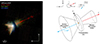 |
Fig. 1. RGB NIRCam images and sketch of the DG Tau B outflow geometry. Left: RGB image of DG Tau B combining three NIRCam exposures in F164N (red) for the [Fe II] 1.64 μm line + continuum, F212N (green) for the H2 1−0 S(1) 2.12 μm line + continuum, and F323N (blue) for the 1−0 O(5) 3.23 μm line + continuum. Right: schematic representation of the DG Tau B disk and outflows showing their orientation and inclination in space. |
The F212N and F323N images show two V-shaped lobes, separated by a dark lane corresponding to the circumstellar obscuration (disk and envelope), as already shown in the HST NICMOS images of Padgett et al. (1999). The eastern blueshifted lobe downward in Fig. 2 shows a similar V-shaped morphology in all images, including F164N, suggesting that the emission is predominantly continuum scattered light. As the wavelength increases the central peak becomes brighter and a point source begins to be distinguished near the origin.
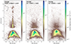 |
Fig. 2. NIRCam narrow-band images of DG Tau B: (a) F164N = continuum + [Fe II], (b) F212N = continuum + H2 1−0 S(1), (c) F323N = continuum + H2 1−0 O(5). The black star at (0, 0) marks the position of the disk continuum emission peak observed with ALMA at 232 GHz (DV20), which is considered to be the source position. The orientation on the sky is shown in panel a. The ΔZ axis points towards the redshifted jet at PA = 295°. |
The receding and much fainter redshifted lobe (upward in Fig. 2) shows a narrow conical geometry in the F212N and F323N filters, not seen in F164N, suggesting that it is tracing in situ H2 emission (as confirmed below by NIRSpec). Around the base of this cone, faint extended emission about 2″ wide, with a similar morphology as in F164N, hence probably due to scattered light (as confirmed by NIRSpec data, Sect. 3.1.2). The base of the lobe is extincted by the disk/envelope. The edges of the receding conical cavity appear brighter than its center and are marginally resolved in the NIRCam images. We estimate their deconvolved thickness at ΔZ = 1.5″ from the central source as ≃0.16″ ± 0.04″ (see Appendix C), corresponding to 22 ± 5 au. The limb-brightening observed suggests a hollow conical geometry for H2, as already observed in CO with ALMA (DV20; DV22).
Turning now to NIRSpec results, we show in Fig. 3 two spectra in the F100LP/G140H and F170LP/G235H bands obtained in a circular aperture of 1.4″ radius centered in the approaching lobe (ΔZ = −0.6″). Twenty-four ro-vibrational H2 transitions are detected, all between 1.1 μm and 3.1 μm. The H2 lines all share the same morphology, which is illustrated in Fig. 4a for the continuum-subtracted H2 2.12 μm emission map. H2 emission stands out more clearly in the NIRSpec observations than in narrow-band NIRCam images due to the combination of spectral resolution and accurate continuum subtraction, demonstrating the performance of NIRSpec-IFU for outflow studies.
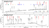 |
Fig. 3. NIRSpec-IFU spectra of DG Tau B. Top panel: spectrum in the F100LP/140H grating integrated over a circular aperture with a radius of 1.4″ centered in the blueshifted lobe containing the central source position (Fig. 4b). Many atomic transitions are detected (in particular for [Fe II]). The mid-band value-free gap is associated with the physical separation between the two NIRSpec detectors. Bottom panel: spectrum in the F170LP/G235H grating integrated in the same circular aperture. Many ro-vibrational H2 transitions are detected, as well as a few [Fe II] and HI atomic transitions. Several photospheric absorption lines, including the CO overtone bands, are observed. The water ice absorption band around 3 μm is clearly visible. The mid-band instrumental gap is also present. |
The redshifted western lobe (pointing upward) shows a narrow conical morphology in H2, strikingly similar to the redshifted CO cavity mapped with ALMA by DV20, shown for comparison in Fig. 4d. Substructures can also be seen as internal arc-shaped enhancements and brightness asymetries along the cavity edges. The blueshifted eastern lobe (pointing downward) shows a wider conical morphology in H2, with multiple bright peaks along the cone walls and down the cone axis. Both H2 lobes appear brighter in their inner ∼1.5 − 2″ region, with a sharp brightness decrease (factor 2−3) beyond. Both are surrounded by a fainter and broader halo of H2 signal.
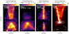 |
Fig. 4. NIRSpec and ALMA maps of DG Tau B outflows. Panel a: NIRSpec H2 1−0 S(1) λ2.12 μm integrated surface brightness map, continuum subtracted. Panel b: NIRSpec average continuum map estimated over a spectral width 1.8 × 10⁻² μm centered on the H2 1−0 S(1) line. The white dashed circle corresponds to the aperture used to extract the spectra from Fig. 3. Panel c: NIRSpec [Fe II] λ1.64 μm integrated surface brightness map, continuum subtracted. Panel d: moment 0 map of the 12CO(2−1) emission observed with ALMA, integrated between (V − Vsys) = +2.15 km s−1 and 8 km s−1. The contours of the ALMA disk continuum at 232 GHz are superimposed. Adapted from DV20. The gray star at offset (0, 0) marks the position of the disk continuum emission peak, considered to be the source position. The ΔZ axis points towards the redshifted jet at PA = 295°. |
For comparison, we plot in Fig. 4b an image of the local continuum level in the vicinity of the H2 2.12 μm transition. Very extended emission is observed, tracing photons from the central continuum source that are scattered by surrounding dust grains. In the redshifted lobe, the continuum map morphology is strikingly different from the bright H2 cone: it traces a broader nebulosity of width ΔR ≃ 2″ emerging from the dark lane and detected out to ΔZ = 2″, similar to the nebulosity observed in the narrow-band images in Fig. 2. In the blueshifted lobe, in contrast, the V-shaped continuum map morphology is very similar to the region of bright H2 in the continuum-subtracted map of Fig. 4a, indicating a stronger contribution of scattered H2 in that lobe. In the next section we attempt to quantify the contribution of scattered versus in situ H2 emission.
3.1.2. Scattered versus in situ H2
As discussed in Sect. 3.1.1, the similar morphology of the blueshifted lobe in all NIRCam images, and in the continuum and H2 NIRSpec maps, indicates a significant contribution of scattering to the total observed intensities. We investigate below the relative importance of scattering and in situ H2 emission using the NIRSpec emission maps. We concentrate on the H2 1−0 S(1) transition at 2.12 μm, which shows the best signal-to-noise ratio (S/N).
We quantify the effect of scattering on H2 by estimating the ratio between the line and adjacent continuum for each spaxel in the NIRSpec data cube. The resulting ratio map is shown as background colors in Fig. 5. Only spaxels where both the line and continuum are detected with a S/N ≥ 3 are considered. If the extended H2 “emission” is dominated by scattering by surrounding dust of bright H2 in the central source spectrum, the line-to-continuum ratio should be uniform over the image. In the case of in situ H2 line emission, the ratio should increase locally. To guide the eye, we superpose in Fig. 5 a contour map of the local continuum level (from Fig. 4b).
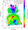 |
Fig. 5. NIRSpec H2 line to continuum map. The color map shows the flux ratio between the 1−0 S(1) H2 line and the local continuum. The ratio is computed for a S/N > 3 in both line and continuum. Black contours plot the continuum map. Levels start at 4σ (with σ = 1.4 × 10⁻³ erg s−1 cm−2 μm−1 sr−1) and increase by a factor of 2. Solid red lines show the projected inner and outer limits of the bright CO cone derived by DV22. |
Towards the redshifted lobe, a wide component with constant line to continuum ratio ∼1 − 2 (green shades) is detected on both sides of the conical flow, coincident with the nebulosity seen in the continuum map, and with a faint halo in the H2 map (Fig. 4a). It appears unlikely that this component traces in situ H2 emission as its spatial distribution coincides with the continuum. This region may trace scattering of H2 from the inner disk and/or from the strong in situ H2 emission associated with the conical red lobe. Interestingly, this nebula is wider than the limits of the bright CO conical outflow as determined by DV22 (shown as red lines in Fig. 5) and extends into the lower velocity wide CO outflow mapped by DV20. In contrast, inside the bright cone of H2, the line to continuum ratio is distinctively higher than in the surrounding nebula, with values of 5−10 that increase away from the source. From this, we estimate that the scattering contribution in H2 is at most 30% at the base of the redshifted conical lobe and less than 15% beyond projected distances of ΔZ = 1.3″ (=180 au).
The H2 emission in the blue, eastern lobe is much more affected by scattering. The regions with substantial continuum emission (see black contours in Fig. 5) exhibit a surprisingly broad range of H2 line-to-continuum ratios. A large fraction of the spaxels have ratio values around 1 − 2 (green shades) similar to those observed in the nebula around the red lobe, suggesting a large contribution from scattered H2. However, some regions near the apex and along the V-shaped cavity walls have much smaller line-to-continuum ratios of 0.2 − 0.3, complicating the interpretation. One possibility might be that the illuminating H2 source is offset from and/or more extended than the continuum, meaning that it does not illuminate the innermost cavity walls in the same way. However, until the origin of this spatial variation in line-to-continuum ratio is fully understood and modeled, however, only the (small) patches in the blue lobe with large ratio values > 5 can be unambiguously considered as dominated by intrinsic in situ H2 emission.
In the remainder of this paper, we therefore focus our analysis on the redshifted (western) lobe, where the contribution of scattering is negligible inside the bright H2 cone. This will enable us to compare quantitatively H2 in situ emission properties with the redshifted CO cavity studied by DV22.
3.1.3. SINFONI velocity map
Thanks to wavelength recalibration on OH sky emission lines (Sect. 2.3, Appendix B) and a higher spectral resolution (∼67 km s−1), the SINFONI data can be used to constrain the radial velocity of H2 more precisely than with NIRSpec.
We first attempted to correct the SINFONI H2 1−0 S(1) spectra for scattering based on the line to continuum ratio, taking the spectrum with the minimum value of this ratio in the SINFONI data as a reference. This is our best estimate of the central source spectrum. At each spaxel position, we then rescaled this reference spectrum to the local continuum level and subtracted from the current spectrum. This method only corrects for the contribution of scattering of the central reference spectrum at each spatial position and may underestimate the scattering contribution in the blue lobe from a more extended H2 source (see discussion in previous section).
Figure 6 shows the intensity and centroid velocity maps of the H2 1−0 S(1) transition, derived from the SINFONI observations corrected (in part) for scattering as described above. Centroid velocities are estimated from a Gaussian fit of the line profiles. Only values corresponding to a line peak S/N > 10 are considered. The blueshifted lobe exhibits radial velocities between −3 and −13 km s−1. However, the light blue regions at low radial velocities close to the source may still be affected by scattering, which biases the estimate of centroid velocities. The redshifted lobe shows more uniform radial velocities with an average value of ∼10 km s−1 and a dispersion of 3 km s−1 rms. In both lobes, no transverse velocity gradient is detected at the 3σ level above ≃3 km s−1, that is, at the level of the residual calibration systematic effects (see Appendix B). We therefore take ΔV = 3 km s−1 as a conservative upper limit for transverse radial velocity gradients. We discuss in Sect. 4.2 the constraints on H2 kinematics (vertical and rotational motions) derived from these measurements.
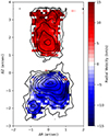 |
Fig. 6. Map of H2 1−0 S(1) centroid velocities from SINFONI observations. Only values for which the S/N > 10 at the line peak are shown. The black contours represent the SINFONI integrated, continuum subtracted H2 1−0 S(1) surface brightness map. Contour levels are 3, 5, 8, 11, 17, 26, 38 and 50σ with σ = 4 × 10⁻⁶ erg s−1 cm−2 sr−1. |
3.2. Atomic jets
The top panel of Fig. 3 shows that the 0.97−1.81 μm wavelength range in NIRSpec observations is dominated by atomic lines, tracing the bipolar jets. We detect transitions of [C I], [S II], [N I], [P II], [O I], He I as well as 17 lines of [Fe II]. Figure 4c shows an example of a NIRSpec continuum-subtracted map in the [Fe II] 1.64 μm transition. The local continuum was removed through a baseline fit to the individual spectra. The redshifted jet morphology is the same as in the F164N NIRCam image (Fig. 2a). However, the blueshifted jet is much more visible in the NIRSpec image (Fig. 4c), thanks to the accurate subtraction of the strong continuum emission in that lobe. The two jet lobes are collimated and well aligned. The inner regions of the receding jet are obscured by the dark lane. The emission peak at 1.64 μm in the [Fe II] NIRSpec map (Fig. 4c) corresponds to an emission knot in the receding jet located at ΔZ ≃ 1.4″. Wider and fainter nebulosity remains visible, even after continuum subtraction, around the base of the receding jet. This nebulosity likely traces scattering of in situ [Fe II] jet emission by the dusty nebula surrounding the base of the jet/outflow, similarly to what is seen in H2 (Fig. 5).
We estimate the position angle (PA) of the redshifted jet by fitting a Gaussian function to each transverse intensity profile in Fig. 2a, at PAjet, red = 295.0° ±0.2°. This value is identical to the PACO, red = 295.0° ±1° of the redshifted CO outflow derived by DV22 and perpendicular to the large-scale disk mapped with ALMA at PAdisk = 25.7° ±0.3° (DV20). Our result is also consistent with the PA values between 273° and 302.5° determined at large distance from the star by Eislöffel & Mundt (1998) for the red knots observed in [S II] 6716,6731 Å.
3.3. Central source
In the NIRCam F164N image, the peak of the disk millimetric continuum is located near the apex of the approaching lobe, consistent with the expected projection effects. As wavelength increases, the NIR emission peak approaches the millimetric intensity maximum. This drift suggests that the source is not seen directly at wavelengths shorter than 3 μm but through continuum scattering by surrounding dust. At short wavelengths, the central source emission is completely absorbed by the dust grains in the envelope and upper layers of the flared disk atmosphere, producing the dark lane. The large-scale continuum emission is dominated by scattered light. As the wavelength increases, the opacity of the dust decreases and so does the width of the occulting dark lane, thereby revealing emission closer to the source position. This effect is illustrated in the Class I model images computed by Whitney et al. (2003, see their Fig. 11).
The NIRSpec spectrum of the blue lobe in the bottom panel of Fig. 3 shows photospheric absorption lines compatible with an early K type (e.g., Si I, Ca I transitions at ∼1.98 μm and ∼2.26 μm, Mg I transitions at ∼2.28 μm). The first three overtone ro-vibrational bands of 12CO (2−0, 3−1 and 4−2) are also detected in absorption between 2.29 and 2.38 μm. A more detailed study of the central star spectrum will be conducted in a forthcoming publication.
3.4. Hydrogen lines and accretion rate
In addition to the main jet and outflow tracers, 11 HI transitions, considered to be accretion tracers, are detected across the 0.97 μm–3.17 μm spectral range (see Fig. 3). All these transitions share a similar extended morphology, illustrated in Fig. 7 with the continuum-subtracted Brγ emission map. The contours of the adjacent continuum are also shown for comparison.
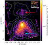 |
Fig. 7. NIRSpec HIcontinuum-subtracted Brγ surface brightness map (color map). White contours plot the continuum near 2.16 μm. Contour levels start at 3σ (σ = 2.3 × 10⁻³ erg s−1 cm−2 μm−1 sr−1) and increase by factors of 2. The ALMA 232 GHz peak continuum position is represented with a black star. The red and blue arrows show the base of the redshifted and blueshifted jets respectively. |
In the approaching lobe, the Brγ emission mostly follows the spatial distribution of the continuum, except for some faint component along the blueshifted jet (see blue arrow, Fig. 7). In particular, the Brγ emission peak overlaps with the continuum intensity maximum. This suggests that most of the HI emission is formed close to the source and scattered along the walls of the V-shaped, blueshifted cavity. In the redshifted lobe, the HI emission traces the base of the receding jet (see red arrow, Fig. 7).
As matter accretes, energy is released in the form of accretion luminosity Lacc. To estimate it, we use the empirical relations between Lacc and (dereddened) luminosity of near-infrared HI emission lines first established by Muzerolle et al. (1998) and recently updated by Alcalá et al. (2017). In the same way as Fiorellino et al. (2021), we assume that the relations remain valid for Class I stars. We use the following 4 HI transitions: Paδ 7−3 at 1.00 μm, Paγ 6−3 at 1.09 μm, Paβ 5−3 at 1.28 μm and Brγ at 2.16 μm. We derive their fluxes in an aperture of radius 2.2″ centered on the continuum peak position. We assume here that all the flux within the aperture comes from an unresolved central source exclusively as the jet contribution is negligible (see Fig. 7). We then derive the best estimate of reddening that yields the same Lacc (and accretion rate) for all dereddened line fluxes, using the empirical relations from Alcalá et al. (2017). Details on the method can be found in Appendix D. We find an extinction AV = 13 ± 4 mag and an accretion rate Ṁacc = 1.0 ± 0.5 × 10⁻¹⁰ M⊙ yr−1. Assuming that the accretion rate onto the star is ten times the red jet mass flux derived by Podio et al. (2011) (Ṁjet = 6.4 × 10⁻⁹ M⊙ yr−1) we expected an accretion rate of ∼6 × 10⁻⁸ M⊙ yr−1. Our Ṁacc estimate is 600 times smaller, suggesting that we are massively underestimating the intrinsic luminosity of HI transitions. Such a discrepancy is unlikely to be due to time variability. Indeed, Podio et al. (2011) show that the redshifted jet mass-loss rate has varied by less than a factor 3 over a period of ∼60 years, suggesting small variations in accretion rate as well.
As discussed before, the bulk of the HI Brγ emission follows the same spatial distribution as the continuum. Therefore, a likely explanation for the discrepancy is that a large fraction of the HI emission coming from the source is occulted, and only a small fraction (≃1/600) is reaching us via scattering into the line of sight. Our method only gives the extinction between us and the last scattering surface of the HI transitions, and therefore severely underestimates the intrinsic line flux. This result shows that extreme care should be taken when estimating accretion rates from HI line fluxes in embedded sources especially at large system inclinations. Similar conclusions have been reached in the recent JWST study of TMC1A by Harsono et al. (2023). The self-consistent approach presented by (Antoniucci et al. 2008; Fiorellino et al. 2021, 2023) should provide a more reliable estimate of the accretion rate, as it uses isochrones (or a birthline) to fully correct for occultation of the central K-band source, and of the associated Brγ emission.
4. Analysis of the redshifted lobe structure
4.1. Jet and H2 opening angle and relation to CO
The H2 emission of the receding lobe appears to be very conical, preserving its opening angle along its axis (Figs. 2b,c and 4a). This morphology is very similar to the bright conical outflow mapped with ALMA on similar scales, where CO traces a hollow conical layer of deprojected inner and outer semi-opening angles of 12.8° and 16.5° respectively (see DV22 and Fig. 8). We estimated the opening angle of the H2 cavity from the NIRSpec data. In order to improve S/N, we used a multiplex H2 map constructed from the 7 most intense transitions: 1−0 S(5) 1.83 μm, 2−1 S(5) 1.94 μm, 1−0 S(3) 1.95 μm, 1−0 S(2) 2.03 μm, 1−0 S(1) 2.12 μm, 1−0 S(0) 2.22 μm, 1−0 O(3) 2.80 μm. As the edges of the H2 cavity are brighter than the center, we estimated their position accurately using a Gaussian fit to the transverse intensity profile, independently on the two sides. By fitting the derived edge positions with a linear function, we estimate the H2 projected semi-opening angle to be 10.4° ±0.5° (deprojected semi-opening angle equal to 9.4° ±0.4°, corresponding to Z/R ≃ 6). These results are shown in Fig. 8. The H2 emitting layer is nested just inside the CO conical cavity. Extrapolating the H2 edge positions to the source, we derive an upper limit on the H2 cavity anchoring radius in the disk of r0, H2 ≤ 6 au.
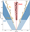 |
Fig. 8. Collimation of the DG Tau B redshifted outflows. The orange dots show the derived positions of the H2 edges from the NIRSpec map. The red filled area indicates the full jet opening angle and the red dots trace the jet axis positions both derived from the F164N NIRCam image. The filled blue conical area show the projected outlines of the outer and inner limits derived by DV22 for the bright conical CO outflow. The light blue areas below ∼180 au correspond to the extrapolated CO flow edges, where no measurements are available. All error bars are 3σ. The double yellow arrow shows the thickness of the H2 cavity estimated in Sect. 3.1.1. |
From the NIRCam F163N image in Fig. 2a we can also precisely constrain the position of the jet axis and its width as a function of distance from the star. Each transverse intensity cut is fitted with a Gaussian profile to estimate an FWHM, which we consider to be the width of the jet, and a center position used to estimate the jet axis position. Small amplitude jet axis wiggling is visible. However, there is no clear increase of axis displacements with distance from the source as would be expected for a jet axis precession signature and/or orbital motion of the jet source (see for e.g., Masciadri & Raga 2002). We estimate a maximum precession angle of 1°. The measured jet FWHM are corrected for the PSF FWHM (0.056″ for the F164N filter3). We estimate a jet projected semi-opening angle of 1.6° ±0.3° (deprojected semi-opening angle of 1.45° ±0.3°), similar to that estimated by Podio et al. (2011) for the optical jet. This corresponds to a jet deprojected Z/R ratio of ≃40, which is around seven times larger than the ratio estimated for the H2 cavity. Extrapolation at the source gives an upper limit on the jet origin (radius at ΔZ = 0) of r0, jet ≤ 4 au.
The western redshifted DG Tau B ejecta form a layered structure. The [Fe II] jet is significantly more collimated than the H2 emission, itself nested inside the CO outflow. The H2 layer thickness, estimated in Sect. 3.1.1 (cf. horizontal orange arrow in Fig. 8), suggests that there is no gap between the H2 and CO flows. Indeed, the transverse Position-Velocity diagrams in Fig. 1 of DV22 show that the highest velocity CO component is aligned with the H2 opening angle. In contrast, no clear connection is observed between the jet and the H2 lobe on large scale (Z > 150 au). However, if we extrapolate the conical morphologies at the origin, the jet, the H2 emission and the inner CO surface all originate from within radial distances R = 6 au of the central star. The connection between these different components could be established close to the disk mid-plane.
4.2. Constraints on H2 flow velocity and rotation
Using the SINFONI centroid velocity map from Fig. 6, we can estimate the vertical velocity VZ and the specific angular momentum J = RVϕ of the redshifted lobe. Assuming that the flow is axisymmetric, these quantities are given by:
where Vlos is the projected velocity along the line of sight (peak centroid velocities in Fig. 6), R the cavity edge radius at a given Z and i the inclination of the flow axis to the line of sight.
Figure 9a shows the inferred axial velocities Vz obtained, using Eq. (1). The values of R are those estimated in Fig. 8 from the NIRSpec H2 datacube, which more precisely locates the cavity edges thanks to its higher angular resolution. The vertical velocity appears to be constant with height at Vz = 22.5 ± 0.8 km s−1. Assuming that the gas flows along the cavity wall, we then estimate a poloidal velocity Vp = 22.8 ± 2.5 km s−1. The derived Vp for H2 is larger than estimated for the conical CO outflow, ranging between 6 and 14 km s−1 (Fig. 9 of DV22). Podio et al. (2011) estimate the velocity of the redshifted jet at ∼140 km s−1. The layered morphology of the outflow is accompanied by a velocity stratification: the more internal the flow, the more collimated and the larger its vertical velocity.
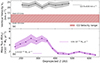 |
Fig. 9. Vertical velocity and mass flux of hot H2 along the redshifted lobe of DG Tau B. (a) Vz as a function of deprojected distance Z from the source, derived from H2 1−0 S(1) SINFONI/VLT observations. For comparison, the shaded red area shows the range of Vz across the CO redshifted conical flow, from outer to inner streamlines DV20. (b) Mass flux of hot H2 as a function of Z (see text). |
Regarding rotation signatures in the H2 outflow, we derive in Sect. 3.1.3 upper limits of ΔV ≤ 3 km s−1 for ΔZ ≥ 200 au. Using Eq. (2) and the H2 cavity radius R(Z), we estimate an upper limit for the specific angular momentum beyond ΔZ = 250 au of J = RVϕ ≤ 90 au km s−1. We will discuss in Sect. 5 the implications brought by the hot H2 kinematics on the MHD disk wind scenario.
4.3. H2 excitation conditions: Extinction, temperature, column density, and mass flux
Numerous ro-vibrational H2 transitions are detected in both lobes. To estimate a column density and excitation temperature in the redshifted lobe, we use the excitation diagram method, assuming optically thin emission (a good assumption for H2 emission in outflows). Thanks to the very good S/N of the lines, the excitation diagrams can be studied at different positions along the flow axis (using typically 18 H2 ro-vibrational lines at each position, see Appendix F).
To increase S/N, we averaged all spaxels with S/N > 3 in the transverse direction perpendicular to the flow axis, and further average over 2 spaxels in the Z-direction. Figure 10a shows the average H2 1−0 S(1) surface brightness distribution inside each of these “slices” as a function of distance along the flow axis. The error bars correspond to the dispersion of values among spaxels in a given slice.
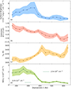 |
Fig. 10. H2 excitation conditions along the redshifted lobe axis. Panel a: surface brightness of H2 1−0 S(1) averaged across the lobe, not corrected for extinction, as a function of deprojected distance from the source. Panel b: average extinction at 2.12 μm obtained from the line ratio H2 1−0 Q(7)/1−0 S(5) (see text). Panel c: H2 excitation temperature obtained by fitting the excitation diagram. Panel d: H2 column density calculated from the same excitation diagrams (see Appendix F). |
We then estimated the mean extinction towards each slice from the H2 line ratio 1−0 Q(7)/1−0 S(5) (at λ = 2.4999 μm and 1.8357 μm respectively). Since these transitions are emitted from the same upper energy level (v = 1, J = 7), their intrinsic ratio is independent of excitation temperature and column density, and is only set by the ratio of their Aij/λ (with Aij the Einstein coefficient), equal to 0.472. Any observed deviation from this value is caused by differential reddening between the wavelengths of the two lines. We adopt the near-infrared extinction law from Wang & Chen (2019):
with α = 2.07 ± 0.03 (for RV = 3.16 ± 0.15). The extinction A2.12 μm at λRef = 2.12 μm can then be expressed as:
with ![$ C_{\lambda_{\mathrm{S5}}, \lambda_{\mathrm{Q7}}} = \left[\left(\frac{2.12}{1.83}\right)^{2.07} - \left(\frac{2.12}{2.49}\right)^{2.07}\right]^{-1} = 1.565 $](/articles/aa/full_html/2024/08/aa49176-24/aa49176-24-eq7.gif) .
.
Figure 10b shows the derived extinction values at 2.12 μm in each slice as a function of distance to the source. A systematic decrease is observed, from a maximum value around 0.9 mag close to the source (ΔZ ≃ 150 au) to negligible values at 600 au. Using Eq. (3), the corresponding optical extinction in the V-band at 0.55 μm is AV = A2.12 (2.12/0.55)α, which gives AV = 14.7 ± 2.3 mag. The maximum extinction derived from the H2 line ratio at Z ≃ 100 − 150 au in the red lobe is comparable to the average extinction estimated towards the blue lobe from the HI lines in Sect. 3.4 (AV = 13 ± 4 mag). These comparable values on similar spatial scales suggest that there is a large-scale circumstellar environment obscuring light in the same way for both lobes of the system.
This extinction profile cannot be caused by the CO conical outflow. In that case, we would expect values typically 10 times lower than those estimated here (see Appendix E). An additional component is required. In Appendix E, we show that a free-falling spherical envelope with a mass infall rate of 4.5 × 10⁻⁶ M⊙ yr−1 can reproduce the extinction values along the receding H2 lobe. This value is on the upper end for a Class I source, but very similar to the large envelope infall rate (5 × 10⁻⁶ M⊙ yr−1) derived by Stark et al. (2006) from the modeling of DG Tau B NICMOS/HST images. The broad low-velocity CO outflow evidenced by DV20 around the bright inner CO conical flow could also contribute to the observed extinction.
Using the values of A2.12 μm derived above, and the extinction law in Eq. (3), we then build dereddened H2 excitation diagrams, averaged over each slice. Only line fluxes with S/N > 3 are considered. No systematic offset between the different vibrational levels v is observed, suggesting that the gas is close to LTE. An excitation temperature Tex and an average column density N(H2) is then estimated for each slice by fitting a straight line (see Appendix F). The last two panels of Fig. 10 show the derived excitation temperature and column density profiles of hot H2 along the redshifted lobe. Tex increases slightly with Z with an average value at Tex ≃ 2200 ± 180 K. Since Tex is relatively constant, the N(H2) profile follows that of the surface brightness with two plateaus: the first one corresponds to an average value of N(H2)≃2 × 1017 cm−2, the second one associated with the fainter part of the cavity, with an average N(H2)∼5 times lower. Assuming that the H2 layer thickness remains constant along the cavity at ΔR ≃ 22 au, and that it is axisymmetric, the average number density of hot H2 molecules in the layer, n(H2) = N(H2)/πΔR, is ∼200 cm−3 within 350 au from the source and 40 cm−3 further out. We stress that this value is only the number density in the form of hot H2 at ∼2000 K; in a PDR layer at T ≃ 2000 K, a low H2 abundance of ≤10−3 is expected (Burton et al. 1990; Bron et al. 2016) so that the total density of H nuclei n(H) could exceed 105 cm−3.
Using the value of Vz estimated in Sect. 4.2 and the column density N(H2) averaged over each slice (from Fig. 10d), it is possible to derive the mass flux in the form of hot H2 along the flow axis:
where Nsp (given in Table F.1) is the number of spaxels inside each slit, of width 2 pixels along the jet axis, and ΔX = 0.1″ is the spaxel size perpendicular to the jet axis, mH the hydrogen mass, Vz the deprojected vertical velocity of the H2 redshifted outflow, and i = 63° the inclination of the disk to the line of sight. Beyond Z = 500 au, we assume that Vz stays constant at the value derived from the SINFONI observations. The H2 mass flux profile shows two plateaus (Fig. 9b), similarly to the column density profile. The mass flux of hot H2 in the inner part of the redshifted lobe is 4.9 × 10⁻¹¹ M⊙ yr−1, decreasing by a factor ∼ 3 beyond Z = 400 au at 1.4 × 10⁻¹¹ M⊙ yr−1. Again we stress that this value is only the mass-flux in the form of hot H2 at ∼2000 K; the total mass-flux carried by this layer will be much larger if hydrogen is mostly atomic; for example, if it traces a dense photodissociated layer in the disk wind (see following section).
5. Discussion
5.1. Global stratified flow structure
Figure 11 summarizes the different components of the DG Tau B outflow. The JWST observations reveal a redshifted H2 flow nested between the fast axial jet and the bright conical CO outflow and extending inwards the radial stratification in velocity and collimation of the CO outflow mapped by DV22. The H2 conical flow is slightly more collimated and two times faster on average than the CO outflow. Its temperature (≃2200 K) and velocity are intermediate between the atomic jet and CO.
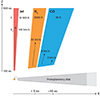 |
Fig. 11. Schematic representation of the layered transverse structure of the DG Tau B redshifted lobe. The variation in opening angle, temperature and poloidal velocity between the atomic jet, the H2 and CO redshifted outflows are illustrated. The different colors describe the temperature gradient in the layers: blue is associated with the coldest component and red with the hottest component. The illustration is not to scale. |
Small-scale H2 outflows have been detected in a few late Class I and high accretion rate Class II sources (Beck et al. 2008; Takami et al. 2007; Agra-Amboage et al. 2014; Melnikov et al. 2023) and recently with JWST in TMC1-A (Harsono et al. 2023) and for 5 young stars by Federman et al. (2024). These outflows all show similar layered structure with wider morphology and lower velocities (V < 30 km s−1 typically) than the axial jets. The blueshifted H2 lobe in DG Tau (Agra-Amboage et al. 2014) in particular shows similarities with the DG Tau B H2 flow, although it is wider (half opening angle of 45°) and much more compact spatially (detected only out to a projected distance of Z = 70 au). The H2 shell in DG Tau extends the onion-like velocity structure observed in atomic lines, tracing the axial jet surrounded by a lower-velocity component (Agra-Amboage et al. 2011; Maurri et al. 2014) and appears nested inside a wide CO outflow (Güdel et al. 2018). Its intrinsic H2 surface brightnesses are however 100 times brighter on average than in the red H2 lobe of DG Tau B.
We discuss below the current constraints from the DG Tau B JWST observations to the three competing scenarios for the origin of these H2 outflows: disk winds versus swept-up cavities versus shocked disk wind.
5.2. MHD disk-wind scenario
The global layered H2/CO structure observed in DG Tau B with temperature, velocity, collimation increasing towards the axis of the flow are reminiscent of a disk wind scenario (as discussed below).
In addition, the derived parameters of the H2 cavity (opening angle, Vz, temperature and to a lesser extent mass flux) appear constant with distance from the source, similar to the CO structure (see DV20; DV22), compatible with an underlying steady ejection process.
We investigate in the following whether the H2 layer could trace inner streamlines of the same disk wind solution that also accounts for the conical CO flow. A photo-evaporative wind is ruled out for the origin of the conical CO flow by the large mass flux (2.3 × 10⁻⁷ M⊙ yr−1) originating from less than 10 au (DV22), which largely exceeds current model predictions (see for example mass-loss compilations in Fig. 7 of Pascucci et al. (2023). A nonthermal acceleration process must therefore be present.
We explore below the case of magnetically driven disk winds. In an MHD disk wind of uniform magnetic level arm the terminal poloidal velocity is proportional to the Keplerian velocity at the streamline footpoint radius r0 (Blandford & Payne 1982; Anderson et al. 2003; Ferreira et al. 2006). Therefore material from inner streamlines will have a higher velocity than material from more external streamlines, reproducing the onion-like velocity layered structure of the DG Tau B redshifted outflows.
The existence of an inner layer of warm (T > 2000 K) molecular gas inside an MHD disk wind, corresponding to the photo-dissociation region, was first predicted by Panoglou et al. (2012). Recent simulations of disk wind outflows by Wang et al. (2019), coupling nonideal magneto-hydrodynamics and thermochemistry, show a layered structure in temperature, velocity and chemical abundance strikingly similar to the H2/CO radial stratification observed in DG Tau B. In their fiducial model, with parameters comparable to the DG Tau B case (disk accretion rate ≃10−8 M⊙ yr−1, stellar mass = 1 M⊙), the wind launched from r = 1 to 100 au stays predominantly molecular except for a thin PDR-like layer of a few 1000 K along the innermost streamlines, where photo-dissociation becomes important. Models of dense photodissociation regions (PDRs) predict that the layer at 2000 K, bright in H2 ro-vibrational emission, would have a low H2 abundance xH2 ≃ 10−3 (Burton et al. 1990; Bron et al. 2016). Taking into account the low H2 abundance, the actual mass-flux along this PDR-like wind layer would then be Ṁ(2000 K) ≃ 1.4 − 5 × 10⁻⁸ M⊙ yr−1.
The H2 flow kinematics and mass-flux bring further constraints to such MHD disk wind solutions. Figure 12 shows the expected relation between the specific angular momentum J = RVϕ and the poloidal velocity Vp in the context of a steady self-similar MHD disk wind solution (Ferreira et al. 2006). As demonstrated in DV22, the layered kinematics of the conical CO outflow is compatible with such an MHD disk wind solution with a constant magnetic lever arm λϕ = 1.58 and streamline anchoring radii r0 ranging between 0.7 and 3.4 au (see blue dots in Fig. 12). We overplot in Fig. 12 the upper limit on J and Vp estimated for the H2 flow in Sect. 4.2. From this diagram, we estimate an upper limit on λH2 < 1.8 and on r0, H2 < 2.0 au.
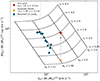 |
Fig. 12. Relation between the poloidal velocity Vp and the specific angular momentum J = RVϕ defining the parameter domain (r0, λϕ) in the case of an MHD disk wind, based on Ferreira et al. (2006). The values obtained by DV22 for the resolved CO redshifted cavity are shown in blue. The red dot is associated with the values of Vp and the upper limit on J estimated by the kinematics study of the H2 redshifted cavity. The yellow point is obtained by considering a constant value of λϕ between the CO and H2 cavities. |
If we assume that the magnetic lever arm parameter remains the same between the H2 and CO outflows, then the observed value of Vp, H2 ≃ 23 km s−1 implies a launching radius r0 = 0.3 au (yellow dot in Fig. 12). The specific angular momentum carried by the H2 flow is then expected to be ≃24 au km s−1, well below our derived upper limit of J ≤ 90 au km s−1. Given the measured H2 flow radii (cf. Fig. 8), expected rotation velocities would be ≤1 km s−1.
In self-similar disk wind solutions, the local ejection efficiency, ξ, is defined as Ṁacc(r ∝ r#x03BE;. If the MHD disk wind dominates the angular momentum extraction from the disk driving accretion, the magnetic lever arm λ is related to ξ with λ ≃ 1 + 1/2ξ (Ferreira 1997). With the assumed value of λ = 1.58 (ξ ≃ 1), the relation between mass accretion rate and radius is simplified to Ṁacc(r ∝ r. Considering the conservation of mass flux across the wind launching region: Ṁw = Ṁacc(r0,out) − Ṁacc(r0,in), the H2 and CO mass fluxes are then linked by a simple expression depending on the respective width of their launching regions:
with Δr0, H2 and Δr0, CO corresponding to (r0, out − r0, in) for the H2 and CO wind launching regions respectively. This relation allows us to eliminate Ṁacc which is poorly constrained in the disk. In the case of the CO conical flow, the kinematic data of DV22 plotted in Fig. 12 give a launching width of Δr0, CO = 3.4 − 0.7 = 2.7 au. With a mass-flux in the CO conical flow of ṀCO = 2 × 10⁻⁷ M⊙ yr−1 (DV22), the total mass flux in the H2 layer at similar distance from the source (Ṁ(2000 K) = 1.4 × 10⁻⁸ M⊙ yr−1 assuming a PDR layer with an H2 abundance of 10−3, see above) can be explained by an H2 wind launching region of Δr0, H2 = 0.2 au in width, which gives launching radii from 0.2 to 0.4 au. This range is consistent with the upper limit on the H2 wind anchoring radius of r0, H2 ≤ 6 au derived from the large-scale morphological study in Sect. 4.1. It is also consistent with the H2 ro-vibrational layer tracing MHD wind streamlines interior to the cold CO conical outflow (launched from r0 ≥ 0.7 au). However, it remains to be checked that PDR models at the derived disk wind densities (nH ≥ 105 cm−3 for H2 abundance ≤10−3 see Sect. 4.3 above) can reproduce the thermalization of the H2 levels for reasonable G0 values and on the spatial scales observed here. We differ this analysis to a forthcoming paper where we combine the NIRSpec and MIRI H2 transitions, providing more stringent constraints to the models. The fact that the H2 emission in the blue lobe appears “knotty” is more difficult to reconcile with an UV irradiated disk wind scenario where the H2 emission may be expected to vary more smoothly, unless different NIR and UV illuminations paths in a clumpy wind are assumed. Alternatively, shocks would be an efficient heating mechanism for the H2 in the disk wind. We discuss this scenario in Sect. 5.4 below.
5.3. Swept-up envelope scenario
The sharp transition in temperature between the adjacent CO and H2 flows, indicated by the small estimated width of the H2 layer (≃20 au width at z = 1.5″), could also arise if the H2 layer is tracing a shocked interface with the surrounding envelope.
The popular analytical model developed by Shu et al. (1991), Lee et al. (2000) of a radially expanding swept-up cavity created by the interaction of an inner wide-angle wind with an outer static stratified environment is unlikely to reproduce the H2 DG Tau B observations, as already argued by DV22 for the CO cavity. Indeed, in such a model, the local shell expansion velocity is proportional to the distance from the source (“Hubble law”), which is not observed here. A similar behavior of self-similar expansion is predicted for the nested magnetic bubbles model presented in Shang et al. (2023) and for the momentum-conserving interaction with an infalling rotating envelope (López-Vázquez et al. 2019).
A variant that avoids this first caveat was presented by Liang et al. (2020). Assuming weak mixing between the shocked wide-angle wind and the shocked ambient gas, a stationary shell is obtained, along which a mixing shear-layer with constant speed can develop. A more serious challenge for swept-up models driven by a wide-angle wind is the small radius of the H2 conical cavity in DG Tau B at its base (< 6 au). The predicted radius reached by the cavity in the disk mid-plane coincides with the centrifugal disk radius López-Vázquez et al. (2019), Liang et al. (2020), which in the case of DG Tau B is at least 750 au (see DV20), much larger than the H2 cavity footpoint radius r0 < 6 au observed here.
Rabenanahary et al. (2022) study entrainment of a stratified static core by a narrow jet (instead of a wide-angle wind) and find it can produce stationary conical cavities with a sheared velocity field similar to the structure of the conical H2/CO layer in DG Tau B. The opening angle and final width depends strongly on the ambient density stratification. Therefore, such a model remains to be computed in the case of more realistic Class 1 environments (including a residual rotating infalling envelope) to see if it could also reproduce the narrow cavity base, large entrained mass-flux in CO and hot H2 along the cavity walls, and large specific angular momentum observed in DG Tau B.
5.4. Shocked disk-wind scenario
An alternative possibility would be that the near-IR ro-vibrational H2 is emitted in the shocked interaction layer driven into an outer disk wind by successive jet bow-shocks, or an inner wide-angle wind. Both models have been recently invoked to reproduce the low velocity SiO shells nested inside the outer SO disk wind in HH212 (Lee et al. 2021, 2022). This scenario differs from the traditional swept-up scenario discussed before in a fundamental way: the cavity in that case is not tracing entrained envelope material but shocked disk wind (plus jet or inner wide-angle wind) material, and the large measured mass-flux has a much stronger, direct implication for disk evolution.
Tabone et al. (2018) simulated numerically the long-term interaction of a time variable jet with a uniform and vertical disk wind. A conical layer forms at the interface by the stacking of multiple bow-shock wings. This jet-disk wind interaction scenario was mentioned by DV22 as a possible alternative for the bright CO cone seen in DG Tau B, which is surrounded by a fainter and slower wind. Possible evidence in support of it was the presence of slight brightness enhancements “substructures” within the CO cone with spacings very similar to the typical spacing of jet knots along the axis, and with linear shapes (as inferred from their velocity gradients) suggestive of shock fronts that could be driven by the impact of recent bow-shock wings against the outer disk wind. The brighter H2 emission at the base of the redshifted cone (< 350 au), coincident with bright inner CO emission could result from the stronger impact of jet bow-shocks close to the source, where both the densities and shock speeds are expected to be higher.
The side-to-side brightness asymmetries seen in the present H2 NIRCam images on the edges of the redshifted cone (with some counterparts in CO; see Figs. 2 and 4) might be additional possible evidence for a jet–disk wind interaction in this system. These asymetries would be naturally explained if the jet undergoes regular precession of its axis. The jet precession angle is constrained at less than 1°. However, DV22 showed that a precession of 0.5° of the conical CO flow axis would be sufficient to reproduce the brightness enhancements seen in CO. Jet precession would not lead to direct impact of the jet on the cavity but rather induce asymmetric bow-shock wings impacting the cavity. However, simulations with more realistic disk wind geometry and kinematics are required for a detailed comparison to observations.
This “shocked disk wind” scenario cannot be fully tested with the near-IR H2 lines alone, as the allowed domain of possible shock conditions is too broad (Agra-Amboage et al. 2014; Kristensen et al. 2023). Stronger constraints will be obtained from the combined analysis of NIRSpec and MIRI data including pure rotational H2 lines, which will be presented in a future publication.
6. Conclusions
In this paper, we present JWST observations of the DG Tau B outflows with NIRCam and NIRSpec-IFU complemented with SINFONI/VLT data to constrain the kinematics. We focus our analysis on the redshifted outflow cavity, which, as seen in ALMA observations, shows properties compatible with a disk-wind origin. Our conclusions can be summarized as follows:
-
The bipolar jet is detected in several atomic tracers ([C I], [S II], [N I], [P II], [O I], He I) but particularly in [Fe II]. The redshifted jet PA is accurately estimated at 295.0° ±0.2°, in full agreement with the PA of the CO redshifted cavity derived by DV22. We derive a jet full-opening angle of 2.9° and an upper limit on the jet radius at its origin of r0, jet ≤ 4 au. The upper limit on the jet axis precession angle is ≤1°.
-
The H2 images show two lobes separated by a dark lane of decreasing thickness with wavelength. The eastern approaching lobe shows a significant contribution from scattered light. As wavelength increases the peak continuum moves closer to the ALMA continuum peak, showing that the source is not seen directly at wavelengths shorter than 3 μm.
-
Estimate of the mass accretion rate onto the star from the dereddened luminosities of HI transitions gives Ṁacc ≃ 10−10 M⊙ yr−1. This is three orders of magnitude smaller than expected from the mass flux of the jet, suggesting that only a tiny fraction (0.1%) of the HI line flux reaches us through scattering. This finding clearly demonstrates that deriving mass-accretion rates from dereddened HI luminosities in embedded sources can lead to severe errors, in particular for highly inclined systems.
-
The H2 redshifted emission shows a narrow conical morphology with a deprojected semi-opening angle 9.4°. Extrapolating at the origin gives an H2 radius on the disk midplane of r0 ≤ 6 au. The H2 emission appears to coincide with the CO cavity inner edge. The atomic jet, the H2 conical wind and the CO conical outflow are nested within each other and form a layered outflow structure.
-
From the SINFONI observations, we derive a constant vertical velocity VZ = 22.5 km s−1 for H2, a factor two larger than the average CO velocity. An upper limit on the H2 specific angular momentum of J < 90 au km s−1 is also derived.
-
A constant H2 excitation temperature T ≃ 2200 K is derived inside the redshifted cavity. The average column density of hot H2 is 2 × 1017 cm−2 close to the source, dropping to 5 × 1016 cm−2 beyond Z = 400 au. The mass flux in the form of hot H2 shows two plateaus at 4.9 × 10⁻¹¹ M⊙ yr−1 close to the source and 1.4 × 10⁻¹¹ M⊙ yr−1 beyond. If ro-vibrational H2 were tracing a dense photodissociated layer, the mass-flux would be a thousand times larger.
The global layered H2–CO structure observed in DG Tau B with temperature, velocity, and collimation increasing towards the axis of the flow is suggestive of an MHD disk-wind scenario. The hot H2 (T ≃ 2000 K) could trace the inner photodissociation layer as predicted by recent simulations. Assuming the same wind magnetic lever arm as for the rotating CO conical outflow (ξ ≃ 1, DV22), an H2 launching region at disk radii of 0.2−0.4 au would account for both the poloidal velocity and the total mass flux. Alternatively, the large jump in temperature between the H2 and CO layers, together with the small thickness of the H2 cavity and the striking conical geometry, might be suggestive of a shocked interface driven by successive jet bow shocks into an outer disk wind (Tabone et al. 2018) or the envelope (Rabenanahary et al. 2022). Dedicated simulations including a more realistic disk wind or infalling envelope will be necessary to test these alternatives. Additional constraints on the H2 excitation processes and cavity formation mechanism will be possible by analyzing the MIRI pure rotational mid-IR H2 transitions, which will be presented in a future publication. The present work clearly demonstrates the unique power of JWST for studies of disk winds in young stars.
The routine is available at: https://github.com/delabrov/JWST-Background-Noise-Removal
Acknowledgments
The authors are grateful and thank the referee for helpful comments that improved the quality of this paper. This work is based on observations made with the NASA/ESA/CSA James Webb Space Telescope. The data were obtained from the Mikulski Archive for Space Telescopes at the Space Telescope Science Institute, which is operated by the Association of Universities for Research in Astronomy, Inc., under NASA contract NAS 5-03127 for JWST. These observations are associated with program #1644 (PI: C. Dougados). This work strongly benefited from the Core2disk-III residential program of Institut Pascal at Université Paris-Saclay, supported by the program “Investissements d’avenir” ANR-11-IDEX-0003-01. This work was supported by the “Programme National de Physique Stellaire” (PNPS) and the Programme National “Physique et Chimie du Milieu Interstellaire” (PCMI) of CNRS/INSU co-funded by CEA and CNES. LP acknowledges the project PRIN MUR 2022 FOSSILS (Chemical origins: linking the fossil composition of the Solar System with the chemistry of protoplanetary disks, Prot. 2022JC2Y93).
References
- Agra-Amboage, V., Dougados, C., Cabrit, S., & Reunanen, J. 2011, A&A, 532, A59 [NASA ADS] [CrossRef] [EDP Sciences] [Google Scholar]
- Agra-Amboage, V., Cabrit, S., Dougados, C., et al. 2014, A&A, 564, A11 [NASA ADS] [CrossRef] [EDP Sciences] [Google Scholar]
- Alcalá, J. M., Manara, C. F., Natta, A., et al. 2017, A&A, 600, A20 [NASA ADS] [CrossRef] [EDP Sciences] [Google Scholar]
- Anderson, J. M., Li, Z.-Y., Krasnopolsky, R., & Blandford, R. D. 2003, ApJ, 590, L107 [Google Scholar]
- Antoniucci, S., Nisini, B., Giannini, T., & Lorenzetti, D. 2008, A&A, 479, 503 [NASA ADS] [CrossRef] [EDP Sciences] [Google Scholar]
- Bai, X.-N., Ye, J., Goodman, J., & Yuan, F. 2016, ApJ, 818, 152 [Google Scholar]
- Beck, T. L., McGregor, P. J., Takami, M., & Pyo, T.-S. 2008, ApJ, 676, 472 [NASA ADS] [CrossRef] [Google Scholar]
- Bjerkeli, P., van der Wiel, M. H. D., Harsono, D., Ramsey, J. P., & Jørgensen, J. K. 2016, Nature, 540, 406 [Google Scholar]
- Blandford, R. D., & Payne, D. G. 1982, MNRAS, 199, 883 [CrossRef] [Google Scholar]
- Bonnefoy, M., Chauvin, G., Lagrange, A. M., et al. 2014, A&A, 562, A127 [NASA ADS] [CrossRef] [EDP Sciences] [Google Scholar]
- Bron, E., Le Petit, F., & Le Bourlot, J. 2016, A&A, 588, A27 [NASA ADS] [CrossRef] [EDP Sciences] [Google Scholar]
- Burton, M. G., Hollenbach, D. J., & Tielens, A. G. G. M. 1990, ApJ, 365, 620 [NASA ADS] [CrossRef] [Google Scholar]
- de Valon, A., Dougados, C., Cabrit, S., et al. 2020, A&A, 634, L12 [NASA ADS] [CrossRef] [EDP Sciences] [Google Scholar]
- de Valon, A., Dougados, C., Cabrit, S., et al. 2022, A&A, 668, A78 [NASA ADS] [CrossRef] [EDP Sciences] [Google Scholar]
- Eislöffel, J., & Mundt, R. 1998, AJ, 115, 1554 [CrossRef] [Google Scholar]
- Erkal, J., Dougados, C., Coffey, D., et al. 2021, A&A, 650, A46 [NASA ADS] [CrossRef] [EDP Sciences] [Google Scholar]
- Federman, S. A., Megeath, S. T., Rubinstein, A. E., et al. 2024, ApJ, 966, 41 [CrossRef] [Google Scholar]
- Ferreira, J. 1997, A&A, 319, 340 [Google Scholar]
- Ferreira, J., Dougados, C., & Cabrit, S. 2006, A&A, 453, 785 [NASA ADS] [CrossRef] [EDP Sciences] [Google Scholar]
- Fiorellino, E., Manara, C. F., Nisini, B., et al. 2021, A&A, 650, A43 [NASA ADS] [CrossRef] [EDP Sciences] [Google Scholar]
- Fiorellino, E., Tychoniec, Ł., Cruz-Sáenz de Miera, F., et al. 2023, ApJ,, 944, 135 [NASA ADS] [CrossRef] [Google Scholar]
- Furlan, E., Watson, D. M., McClure, M. K., et al. 2009, ApJ, 703, 1964 [Google Scholar]
- Garufi, A., Podio, L., Codella, C., et al. 2020, A&A, 636, A65 [NASA ADS] [CrossRef] [EDP Sciences] [Google Scholar]
- Güdel, M., Eibensteiner, C., Dionatos, O., et al. 2018, A&A, 620, L1 [NASA ADS] [CrossRef] [EDP Sciences] [Google Scholar]
- Güver, T., & Özel, F. 2009, MNRAS, 400, 2050 [Google Scholar]
- Harsono, D., Bjerkeli, P., Ramsey, J. P., et al. 2023, ApJ, 951, L32 [NASA ADS] [CrossRef] [Google Scholar]
- Houllé, M., Vigan, A., Carlotti, A., et al. 2021, A&A, 652, A67 [NASA ADS] [CrossRef] [EDP Sciences] [Google Scholar]
- Kimmig, C. N., Dullemond, C. P., & Kley, W. 2020, A&A, 633, A4 [NASA ADS] [CrossRef] [EDP Sciences] [Google Scholar]
- Kristensen, L. E., Godard, B., Guillard, P., Gusdorf, A., & Pineau des Forêts, G. 2023, A&A, 675, A86 [NASA ADS] [CrossRef] [EDP Sciences] [Google Scholar]
- Launhardt, R., Pavlyuchenkov, Y., Gueth, F., et al. 2009, A&A, 494, 147 [NASA ADS] [CrossRef] [EDP Sciences] [Google Scholar]
- Lee, C.-F., Mundy, L. G., Reipurth, B., Ostriker, E. C., & Stone, J. M. 2000, ApJ, 542, 925 [NASA ADS] [CrossRef] [Google Scholar]
- Lee, C.-F., Tabone, B., Cabrit, S., et al. 2021, ApJ, 907, L41 [NASA ADS] [CrossRef] [Google Scholar]
- Lee, C.-F., Li, Z.-Y., Shang, H., & Hirano, N. 2022, ApJ, 927, L27 [NASA ADS] [CrossRef] [Google Scholar]
- Lesur, G. R. J. 2021, A&A, 650, A35 [NASA ADS] [CrossRef] [EDP Sciences] [Google Scholar]
- Liang, L., Johnstone, D., Cabrit, S., & Kristensen, L. E. 2020, ApJ, 900, 15 [NASA ADS] [CrossRef] [Google Scholar]
- López-Vázquez, J. A., Cantó, J., & Lizano, S. 2019, ApJ, 879, 42 [CrossRef] [Google Scholar]
- López-Vázquez, J. A., Lee, C. F., Fernández-López, M., et al. 2024, ApJ, 962, 28 [CrossRef] [Google Scholar]
- Louvet, F., Dougados, C., Cabrit, S., et al. 2018, A&A, 618, A120 [NASA ADS] [CrossRef] [EDP Sciences] [Google Scholar]
- Luhman, K. L., Allen, P. R., Espaillat, C., Hartmann, L., & Calvet, N. 2010, ApJS, 186, 111 [Google Scholar]
- Marconi, A., Axon, D. J., Capetti, A., et al. 2003, ApJ, 586, 868 [Google Scholar]
- Masciadri, E., & Raga, A. C. 2002, ApJ, 568, 733 [Google Scholar]
- Maurri, L., Bacciotti, F., Podio, L., et al. 2014, A&A, 565, A110 [NASA ADS] [CrossRef] [EDP Sciences] [Google Scholar]
- Melnikov, S., Boley, P. A., Nikonova, N. S., et al. 2023, A&A, 673, A156 [NASA ADS] [CrossRef] [EDP Sciences] [Google Scholar]
- Mitchell, G. F., Sargent, A. I., & Mannings, V. 1997, ApJ, 483, L127 [NASA ADS] [CrossRef] [Google Scholar]
- Muzerolle, J., Hartmann, L., & Calvet, N. 1998, AJ, 116, 2965 [NASA ADS] [CrossRef] [Google Scholar]
- Padgett, D. L., Brandner, W., Stapelfeldt, K. R., et al. 1999, AJ, 117, 1490 [CrossRef] [Google Scholar]
- Panoglou, D., Cabrit, S., Pineau Des Forêts, G., et al. 2012, A&A, 538, A2 [CrossRef] [EDP Sciences] [Google Scholar]
- Pascucci, I., Cabrit, S., Edwards, S., et al. 2023, ASP Conf. Ser., 534, 567 [NASA ADS] [Google Scholar]
- Podio, L., Eislöffel, J., Melnikov, S., Hodapp, K. W., & Bacciotti, F. 2011, A&A, 527, A13 [NASA ADS] [CrossRef] [EDP Sciences] [Google Scholar]
- Pudritz, R. E., Rogers, C. S., & Ouyed, R. 2006, MNRAS, 365, 1131 [NASA ADS] [CrossRef] [Google Scholar]
- Rabenanahary, M., Cabrit, S., Meliani, Z., & Pineau des Forêts, G. 2022, A&A, 664, A118 [NASA ADS] [CrossRef] [EDP Sciences] [Google Scholar]
- Rauscher, B. J., Arendt, R. G., Fixen, D. J., et al. 2011, SPIE Conf. Ser., 8155, 81550C [NASA ADS] [Google Scholar]
- Riols, A., & Lesur, G. 2018, A&A, 617, A117 [NASA ADS] [CrossRef] [EDP Sciences] [Google Scholar]
- Shang, H., Liu, C.-F., Krasnopolsky, R., & Wang, L.-Y. 2023, ApJ, 944, 230 [NASA ADS] [CrossRef] [Google Scholar]
- Shu, F. H., Ruden, S. P., Lada, C. J., & Lizano, S. 1991, ApJ, 370, L31 [NASA ADS] [CrossRef] [Google Scholar]
- Stapelfeldt, K., Burrows, C. J., Krist, J. E., & WFPC2 Science Team 1997, in Herbig-Haro Flows and the Birth of Stars, eds. B. Reipurth, & C. Bertout, 182, 355 [NASA ADS] [CrossRef] [Google Scholar]
- Stark, D. P., Whitney, B. A., Stassun, K., & Wood, K. 2006, ApJ, 649, 900 [NASA ADS] [CrossRef] [Google Scholar]
- Sturm, J. A., McClure, M. K., Beck, T. L., et al. 2023, A&A, 679, A138 [NASA ADS] [CrossRef] [EDP Sciences] [Google Scholar]
- Tabone, B., Cabrit, S., Bianchi, E., et al. 2017, A&A, 607, L6 [NASA ADS] [CrossRef] [EDP Sciences] [Google Scholar]
- Tabone, B., Raga, A., Cabrit, S., & Pineau des Forêts, G., 2018, A&A, 614, A119 [CrossRef] [EDP Sciences] [Google Scholar]
- Takami, M., Beck, T. L., Pyo, T.-S., McGregor, P., & Davis, C. 2007, ApJ, 670, L33 [NASA ADS] [CrossRef] [Google Scholar]
- Wang, S., & Chen, X. 2019, ApJ, 877, 116 [Google Scholar]
- Wang, L., Bai, X.-N., & Goodman, J. 2019, ApJ, 874, 90 [Google Scholar]
- Whitney, B. A., Wood, K., Bjorkman, J. E., & Cohen, M. 2003, ApJ, 598, 1079 [CrossRef] [Google Scholar]
- Zapata, L. A., Lizano, S., Rodríguez, L. F., et al. 2015, ApJ, 798, 131 [NASA ADS] [CrossRef] [Google Scholar]
Appendix A: Correction of 1/f correlated noise in NIRSpec and NIRCam data
All JWST instruments, for example NIRISS, MIRI, and in particular NIRSpec and NIRCam, are connected to a pixel reading device called SIDECAR ASIC. As a result, all the detectors on all the instruments suffer from correlated 1/f read-out noise (Rauscher et al. 2011). It is quite complicated to fully correct the contribution of this noise in the images due to the stochastic mechanisms at its origin, but we propose a simple method that significantly reduces its impact on both NIRCam and NIRSpec datasets.
The most obvious property of 1/f noise in images is the appearance of "banding". These bands stand out from the standard dispersion of the image background. For example, in the case of NIRSpec, the frames of the NRS1 and NRS2 detectors are covered by vertical "bands". The method used here4 applies to both NIRSpec and NIRCam observations and works on the output files from step 1 of the JWST pipeline (Detector1) named with the suffix "_rate". Applying this method does not modify the file structure in any way. It is then possible to restart the rest of the pipeline using these corrected files as input files for the "Spec2" or "Image2" stage.
To correct the banding effect, an average value is estimated for each slit in the image. This average value is estimated by applying a σ-clipping method. The σ value is estimated from the histogram of the image pixel distribution. A clipping value of 1.5σ has been found optimum and was applied to all the images presented in this article.
Fig. A.1 shows an example of the results obtained for the NIRSpec IFU NRS2 detector in the F100LP/G140H configuration. The left image shows a raw image output by Detector1 before correction, with the characteristic “bands” of 1/f noise. The second figure shows the image obtained after noise correction. The subtracted flux values used are shown in the smaller middle image. It can be seen that the bands are for the most part relatively well subtracted, increasing the S/N of the spectra present in the image. We can also see that the horizontal dispersion of the image is reduced by the correction, without altering the average value of the vertical slits.
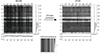 |
Fig. A.1. Illustration of the 1/f noise correction. Example of an image from NIRSpec NRS2 detector before (left) and after (right) correction for 1/f correlated noise. The box to the right of each image plots the median values of each horizontal slit in the image. The boxes at the bottom show the median values of each vertical slit in the image. The smaller image in the middle corresponds to the map of mean values subtracted from the initial image. |
Appendix B: SINFONI precise wavelength calibration method using atmospheric lines
In the SINFONI observations, after processing with the reduction pipeline, a systematic offset in radial velocity (RV) of ∼40 km s−1 is observed in the OH telluric emission lines in all the spaxels. Since the aim of the SINFONI observations is to study the kinematics of the H2 ejecta, we perform a spectral recalibration of the datacube in order to constrain the H2 radial velocities more precisely.
The method used is based on the cross-correlation between the individual spectra of the data cube and a theoretical atmospheric spectrum containing the telluric lines emitted in the spectral band of our observations. This atmospheric model is obtained from ESO’s Sky Model Calculator5 tool by specifying the date and conditions of the observations. This analysis is applied to the data cube reduced with the pipeline but deactivating sky correction so that OH sky emission lines are preserved. The cross-correlation routine used on our data is taken from the TexTRIS python module (Bonnefoy et al. 2014), a package tailored to the processing of raw SINFONI data.
The cross-correlation between the current spectrum and the reference atmospheric spectrum is computed at each spaxel position of the datacube. The cross-correlation is sampled every 0.2 km s−1. Its maximum gives the estimated radial velocity correction RV to be applied at the current spaxel position. The TexTRIS routine returns the S/N associated with the cross-correlation curve (Houllé et al. 2021), which makes it possible to estimate offset errors via the relation:
σ the width of the cross-correlation profile estimated by a Gaussian fit. The derived RV offsets map is shown in Fig. B.1. The values vary between +36 and +50 km s−1. We observe a vertical gradient, corresponding to the Uneven Slit Illumination Effect (USIE) (Marconi et al. 2003). This effect occurs when strong gradients of illumination across the SINFONI slitlet direction are present (Erkal et al. 2021). In our case, the pattern reflects the nonuniform illumination due to the DG Tau B continuum emission. Horizontal gradients are also visible along each slitlet direction. These may be due to systematic errors in the spectrum extraction from the detector or to horizontal variations in illumination, which generates a second USIE.
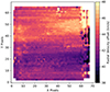 |
Fig. B.1. Map of radial velocity offsets in the SINFONI data cube. The values are estimated via the cross-correlation method over a spectral range between 2.10 and 2.17μm. |
To improve the S/N on the RV correction map, we fit the horizontal gradients with a polynomial function of order between 1 and 3, depending on the variation observed. The resulting fit values are used to build the RV correction map. This RV correction map has been applied to produce the H2 centroid velocity map presented in Fig. 6.
The average resulting fit RMS over the entire frame is 0.35 km s−1, which corresponds to ∼1/100 of the spectral sampling. This corresponds to a typical relative error between spectra on the same SINFONI slitlet direction.
To estimate an absolute error of the RV offsets, we perform the cross-correlation at each spaxel position over several small spectral intervals. This allows us to estimate the variation of the RV offset as a function of the central wavelength of the correlation interval. The derived Δλ offsets are constant with wavelength, which results in RV offsets decreasing linearly with wavelength. By averaging the RMS values of Δλ over all the spaxels of the cube, we estimate an absolute error on the recalibration of 3.5 × 10⁻⁶ μm, which corresponds to a RV offset error equal to ∼0.5 km s−1 at 2.12μm. Combining relative and absolute errors we estimate a final uncertainty of 0.6 km s−1 (1σ) in the global velocity calibration at each spaxel, averaged over all OH lines used for the correlation.
However, this method derives average RV offset values over a wavelength range. By analysing the residual radial velocities of two atmospheric OH transitions adjacent to the 1-0S(1) H2 line, we show that this procedure does not fully correct the offsets at a given wavelength.
Figure B.2 shows the RV offsets difference maps for two OH transitions close to 2.12μm. The ΔRV values are computed as differences between the two RV values at symmetrical distances with respect to the H2 redshifted outflow axis. Residual horizontal velocity gradients are still present that limit our ability to detect rotation in the DG Tau B H2 flow. In the region where the H2 redshifted cavity is located (Y < 30), there are ΔRV gradients in opposite directions between the two maps, on average around 1 km s−1 and going up to 3 km s−1. Therefore, we estimate a conservative 3σ upper limit on ΔRV of ∼3 km s−1 in the DG Tau B redshifted H2 cavity.
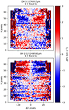 |
Fig. B.2. Top panel: Radial velocity differences ΔRV map of the 9-7 R1(2.5) atmospheric OH line. Bottom panel: Same map for the 9-7 R1(1.5) atmospheric OH line. The X = 0 axis defines the redshifted outflow axis in this figure. ΔRV are constructed by computing the difference between RV values at symmetric X distances from the outflow axis. The redshifted outflow is located in the bottom part of these maps (Y < 30). |
Appendix C: H2 redshifted cavity thickness
The edges of the H2 conical emission in redshifted lobe appear marginally resolved in the NIRCam F212N images. To estimate their thickness, we construct an intensity profile perpendicular to the cavity axis at Z = 1.5″ from the central source. In order to increase the S/N, we summed the profiles over 5 pixels along the flow axis. We checked that this averaging process does not overestimate the thickness by more than 10% due to the conical opening of the cavity. The profile obtained is shown in Fig. C.1. The profile was fit by a function composed of three Gaussians in order to match the wide extended component and the two peaks associated with the bright edges. We derive a H2 cavity thickness of 0.16″ ± 0.04″ (deconvolved quadratically from the FWHM of the PSF6, equivalent to 0.072″ in the F212N filter), corresponding to 22±5 au. Unfortunately, it was not possible to estimate the thickness of the H2 edges at larger distances from the source due to significantly lower S/N in the transverse intensity profiles.
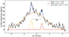 |
Fig. C.1. Measure of the H2 cavity thickness from the NIRCam images. The black curve shows the transverse intensity profile perpendicular to the axis of the redshifted H2 cavity measured on the NIRCam F212N image at ΔZ = 1.5″. The blue curve corresponds to the fit of the profile by a combination of 3 Gaussians. The red and yellow curves are the individual Gaussians fitting the two intensity peaks associated with the bright edges of the cavity. The orange curve corresponds to the fit of the wide baseline component. The gray line, called "CW" for Cavity Width, shows the separation between the two Gaussian center positions. |
Appendix D: Accretion rate onto the star from dereddening of HI lines
The accretion rate is estimated using 4 HI transitions, those with the best S/N in the spectra: Paδ 7-3 at 1.00μm, Paγ 6-3 at 1.09μm, Paβ 5-3 at 1.28μm and Brγ at 2.16μm. The fluxes considered for estimating the accretion luminosities are obtained in a circular aperture of diameter 1.2″ centred in the blue lobe and containing the central source position. This aperture encloses all HI Brγ flux above the 3σ detection limit. The observed fluxes are listed in Table D.1, together with the parameters a and b of the empirical relations in Alcalá et al. (2017) of the shape: log(Lacc/L⊙) = alog(LHI/L⊙)+b, where LHI is the dereddened luminosity of each line. By using 4 HI transitions at different wavelengths, and the extinction curve of Wang & Chen (2019), we can find the value of AV that gives the same Lacc for the 4 derredened line fluxes. The accretion rate is then deduced from the accretion luminosity by the relation Ṁaccc = LaccR∗/(GM∗) considering the DG Tau B parameters as follows: R* = 2 R⊙ and M* = 1.1M⊙ (DV20).
HI transitions used in accretion rate estimation.
Figure D.1 shows the estimated accretion rates from the 4 HI lines considered as a function of the extinction AV. The curves intersect at approximately the same values: Av = 13 ± 4 for Ṁacc = (1.0 ± 0.5) × 10−10 M⊙ yr−1. The errors correspond to the average dispersion of the values for each intersection of two curves.
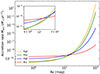 |
Fig. D.1. Accretion rate Ṁacc as a function of extinction AV reproducing the observed fluxes of the atomic transitions HI Paδ, Paγ, Paβ and Brγ. The curves are derived from the empirical relations between Lacc and LHI of Alcalá et al. (2017). The intersection of the four curves gives the best estimate of Ṁacc and AV towards DG Tau B. |
Appendix E: Extinction caused by the CO conical outflow and an envelope in free-fall
From the analysis of the excitation diagrams in Sect. 4.3 we estimate the extinction between us and the H2 emission along the redshifted lobe axis. The aim here is to compare to the extinction due to the CO conical outflow, and to an envelope in free-fall.
E.1. CO conical outflow
de Valon et al. (2020) estimates a constant total mass flux along Z in the CO redshifted conical outflow of 2.2 ± 0.7 × 10⁻⁷ M⊙ yr−1. From this value and considering the average CO ejection velocity, we can estimate the mass in a slice of thickness ΔZ as:
VZ, real is the CO deprojected velocity and Rout and Rin are respectively the radii associated with the edges of the CO conical flow at a given Z position. Figure E.2 illustrates the considered geometry and the definition of Rin and Rout. The subscript "real" means that the quantities are deprojected, considering the angle of inclination i = 63° of the DG Tau B flow axis with respect to the line of sight, as opposed to projected quantities annotated with "proj". From these quantities we can derive the hydrogen column density NH as:
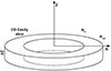 |
Fig. E.1. Illustration of a slice of the CO redshifted conical outflow perpendicular to its axis. If the slice is sufficiently thin, it can be approximated as a hollow cylinder of thickness ΔR = Rout − Rin. |
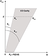 |
Fig. E.2. Cutout in the (R, Z) plane of the CO conical redshifted outflow defined by its two opening angles θin and θout and having the parameter R0 as its external anchoring radius in the disk. These parameters are as derived in DV22. |
And the projected values of Z and the radii are defined as:


Rin corresponds to the extrapolated internal radius of the CO conical outflow, defined from the internal deprojected opening angle θin equal to 12.8° and Rout being the external radius of the conical outflow, using the deprojected external opening angle θout of 16.5° (Rin(Z = 0) = 0 and Rout(Z = 0) = 40 au, values taken from Fig. 9 of DV22).
From this column density profile NH(Z), we can estimate the extinction associated with the CO conical flow using the Güver & Özel (2009) relation: NH(cm−2) = (2.21 ± 0.09)×1021AV. The extinction profile obtained is shown in Fig. E.3. The profile is inversely proportional to Z (due to the fact that R ∝ Z since the cavity is considered to be conical). Extinctions are given at 2.12μm, which is more consistent since we are working in the near infrared. The conversion between AV and A2.12μm is made via the power law given in Eq. 3, from Wang & Chen (2019).
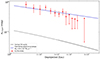 |
Fig. E.3. Predicted reddening variation along the DG Tau B redshifted lobe for the conical CO outflow and envelope. The red points are the extinction values estimated from the H2 ro-vibrational transitions in Sect. 4.3. The black curve shows the expected extinction at 2.12μm as a function of distance from the source due to the CO conical redshifted outflow using the mass flux estimated in DV20. The black dashed curve represents the extrapolation of the model below 300 au assuming a constant CO mass flux. The blue line corresponds to the extinction profile for a spherical envelope in free fall with an infall rate of 4.5 × 10⁻⁶ M⊙ yr−1. |
E.2. Envelope in free-fall
In the same way, we estimate the extinction caused by a spherical envelope free-falling towards the star. The envelope mass infall rate is given by:
where the gas free-fall velocity is given by:
The column density of atomic hydrogen is then expressed as:
Using the relation NH(cm−2) = (2.21 ± 0.09)×1021AV (Güver & Özel 2009), we derive the following relation:
Finally, we convert to A2.12μm ≃ AV/16.3 (see Eq. 3). Figure E.3 plots the profile that best reproduces the extinction values derived from the H2 line ratios, the derived infall rate is Ṁff = 4.5 × 10⁻⁶ M⊙ yr−1.
Appendix F: Excitation Diagrams
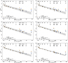 |
Fig. F.1. H2 excitation diagrams at various deprojected distances Z along the redshifted lobe. They are obtained in slits of width ΔZ = 0.2″ (=28 au). Rotational transitions are labeled at the top of each diagram and were dereddened using the mean extinction A2.12μm estimated from the 1-0Q(7)/1-0S(5) line ratio. v = 1 levels are plotted in orange and v = 2 in blue. The opened diamond symbols represent the 3σ upper limits of undetected H2 transitions. Error bars are at 1σ. The gray dashed line is the best fit to the points and the gray area shows the 1σ range. The text at the bottom of each panel gives respectively the deprojected distance Z, the mean extinction A2.12μm, the excitation temperature Tex and the hot H2 column density N(H2) derived from the fit parameters. |
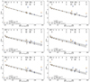 |
Fig. F.1. continued. |
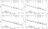 |
Fig. F.1. continued. |
Quantities along the H2 redshifted cavity of DG Tau B.
All Tables
All Figures
|
Fig. 1. RGB NIRCam images and sketch of the DG Tau B outflow geometry. Left: RGB image of DG Tau B combining three NIRCam exposures in F164N (red) for the [Fe II] 1.64 μm line + continuum, F212N (green) for the H2 1−0 S(1) 2.12 μm line + continuum, and F323N (blue) for the 1−0 O(5) 3.23 μm line + continuum. Right: schematic representation of the DG Tau B disk and outflows showing their orientation and inclination in space. |
| In the text | |
|
Fig. 2. NIRCam narrow-band images of DG Tau B: (a) F164N = continuum + [Fe II], (b) F212N = continuum + H2 1−0 S(1), (c) F323N = continuum + H2 1−0 O(5). The black star at (0, 0) marks the position of the disk continuum emission peak observed with ALMA at 232 GHz (DV20), which is considered to be the source position. The orientation on the sky is shown in panel a. The ΔZ axis points towards the redshifted jet at PA = 295°. |
| In the text | |
|
Fig. 3. NIRSpec-IFU spectra of DG Tau B. Top panel: spectrum in the F100LP/140H grating integrated over a circular aperture with a radius of 1.4″ centered in the blueshifted lobe containing the central source position (Fig. 4b). Many atomic transitions are detected (in particular for [Fe II]). The mid-band value-free gap is associated with the physical separation between the two NIRSpec detectors. Bottom panel: spectrum in the F170LP/G235H grating integrated in the same circular aperture. Many ro-vibrational H2 transitions are detected, as well as a few [Fe II] and HI atomic transitions. Several photospheric absorption lines, including the CO overtone bands, are observed. The water ice absorption band around 3 μm is clearly visible. The mid-band instrumental gap is also present. |
| In the text | |
|
Fig. 4. NIRSpec and ALMA maps of DG Tau B outflows. Panel a: NIRSpec H2 1−0 S(1) λ2.12 μm integrated surface brightness map, continuum subtracted. Panel b: NIRSpec average continuum map estimated over a spectral width 1.8 × 10⁻² μm centered on the H2 1−0 S(1) line. The white dashed circle corresponds to the aperture used to extract the spectra from Fig. 3. Panel c: NIRSpec [Fe II] λ1.64 μm integrated surface brightness map, continuum subtracted. Panel d: moment 0 map of the 12CO(2−1) emission observed with ALMA, integrated between (V − Vsys) = +2.15 km s−1 and 8 km s−1. The contours of the ALMA disk continuum at 232 GHz are superimposed. Adapted from DV20. The gray star at offset (0, 0) marks the position of the disk continuum emission peak, considered to be the source position. The ΔZ axis points towards the redshifted jet at PA = 295°. |
| In the text | |
|
Fig. 5. NIRSpec H2 line to continuum map. The color map shows the flux ratio between the 1−0 S(1) H2 line and the local continuum. The ratio is computed for a S/N > 3 in both line and continuum. Black contours plot the continuum map. Levels start at 4σ (with σ = 1.4 × 10⁻³ erg s−1 cm−2 μm−1 sr−1) and increase by a factor of 2. Solid red lines show the projected inner and outer limits of the bright CO cone derived by DV22. |
| In the text | |
|
Fig. 6. Map of H2 1−0 S(1) centroid velocities from SINFONI observations. Only values for which the S/N > 10 at the line peak are shown. The black contours represent the SINFONI integrated, continuum subtracted H2 1−0 S(1) surface brightness map. Contour levels are 3, 5, 8, 11, 17, 26, 38 and 50σ with σ = 4 × 10⁻⁶ erg s−1 cm−2 sr−1. |
| In the text | |
|
Fig. 7. NIRSpec HIcontinuum-subtracted Brγ surface brightness map (color map). White contours plot the continuum near 2.16 μm. Contour levels start at 3σ (σ = 2.3 × 10⁻³ erg s−1 cm−2 μm−1 sr−1) and increase by factors of 2. The ALMA 232 GHz peak continuum position is represented with a black star. The red and blue arrows show the base of the redshifted and blueshifted jets respectively. |
| In the text | |
|
Fig. 8. Collimation of the DG Tau B redshifted outflows. The orange dots show the derived positions of the H2 edges from the NIRSpec map. The red filled area indicates the full jet opening angle and the red dots trace the jet axis positions both derived from the F164N NIRCam image. The filled blue conical area show the projected outlines of the outer and inner limits derived by DV22 for the bright conical CO outflow. The light blue areas below ∼180 au correspond to the extrapolated CO flow edges, where no measurements are available. All error bars are 3σ. The double yellow arrow shows the thickness of the H2 cavity estimated in Sect. 3.1.1. |
| In the text | |
|
Fig. 9. Vertical velocity and mass flux of hot H2 along the redshifted lobe of DG Tau B. (a) Vz as a function of deprojected distance Z from the source, derived from H2 1−0 S(1) SINFONI/VLT observations. For comparison, the shaded red area shows the range of Vz across the CO redshifted conical flow, from outer to inner streamlines DV20. (b) Mass flux of hot H2 as a function of Z (see text). |
| In the text | |
|
Fig. 10. H2 excitation conditions along the redshifted lobe axis. Panel a: surface brightness of H2 1−0 S(1) averaged across the lobe, not corrected for extinction, as a function of deprojected distance from the source. Panel b: average extinction at 2.12 μm obtained from the line ratio H2 1−0 Q(7)/1−0 S(5) (see text). Panel c: H2 excitation temperature obtained by fitting the excitation diagram. Panel d: H2 column density calculated from the same excitation diagrams (see Appendix F). |
| In the text | |
|
Fig. 11. Schematic representation of the layered transverse structure of the DG Tau B redshifted lobe. The variation in opening angle, temperature and poloidal velocity between the atomic jet, the H2 and CO redshifted outflows are illustrated. The different colors describe the temperature gradient in the layers: blue is associated with the coldest component and red with the hottest component. The illustration is not to scale. |
| In the text | |
|
Fig. 12. Relation between the poloidal velocity Vp and the specific angular momentum J = RVϕ defining the parameter domain (r0, λϕ) in the case of an MHD disk wind, based on Ferreira et al. (2006). The values obtained by DV22 for the resolved CO redshifted cavity are shown in blue. The red dot is associated with the values of Vp and the upper limit on J estimated by the kinematics study of the H2 redshifted cavity. The yellow point is obtained by considering a constant value of λϕ between the CO and H2 cavities. |
| In the text | |
|
Fig. A.1. Illustration of the 1/f noise correction. Example of an image from NIRSpec NRS2 detector before (left) and after (right) correction for 1/f correlated noise. The box to the right of each image plots the median values of each horizontal slit in the image. The boxes at the bottom show the median values of each vertical slit in the image. The smaller image in the middle corresponds to the map of mean values subtracted from the initial image. |
| In the text | |
|
Fig. B.1. Map of radial velocity offsets in the SINFONI data cube. The values are estimated via the cross-correlation method over a spectral range between 2.10 and 2.17μm. |
| In the text | |
|
Fig. B.2. Top panel: Radial velocity differences ΔRV map of the 9-7 R1(2.5) atmospheric OH line. Bottom panel: Same map for the 9-7 R1(1.5) atmospheric OH line. The X = 0 axis defines the redshifted outflow axis in this figure. ΔRV are constructed by computing the difference between RV values at symmetric X distances from the outflow axis. The redshifted outflow is located in the bottom part of these maps (Y < 30). |
| In the text | |
|
Fig. C.1. Measure of the H2 cavity thickness from the NIRCam images. The black curve shows the transverse intensity profile perpendicular to the axis of the redshifted H2 cavity measured on the NIRCam F212N image at ΔZ = 1.5″. The blue curve corresponds to the fit of the profile by a combination of 3 Gaussians. The red and yellow curves are the individual Gaussians fitting the two intensity peaks associated with the bright edges of the cavity. The orange curve corresponds to the fit of the wide baseline component. The gray line, called "CW" for Cavity Width, shows the separation between the two Gaussian center positions. |
| In the text | |
|
Fig. D.1. Accretion rate Ṁacc as a function of extinction AV reproducing the observed fluxes of the atomic transitions HI Paδ, Paγ, Paβ and Brγ. The curves are derived from the empirical relations between Lacc and LHI of Alcalá et al. (2017). The intersection of the four curves gives the best estimate of Ṁacc and AV towards DG Tau B. |
| In the text | |
|
Fig. E.1. Illustration of a slice of the CO redshifted conical outflow perpendicular to its axis. If the slice is sufficiently thin, it can be approximated as a hollow cylinder of thickness ΔR = Rout − Rin. |
| In the text | |
|
Fig. E.2. Cutout in the (R, Z) plane of the CO conical redshifted outflow defined by its two opening angles θin and θout and having the parameter R0 as its external anchoring radius in the disk. These parameters are as derived in DV22. |
| In the text | |
|
Fig. E.3. Predicted reddening variation along the DG Tau B redshifted lobe for the conical CO outflow and envelope. The red points are the extinction values estimated from the H2 ro-vibrational transitions in Sect. 4.3. The black curve shows the expected extinction at 2.12μm as a function of distance from the source due to the CO conical redshifted outflow using the mass flux estimated in DV20. The black dashed curve represents the extrapolation of the model below 300 au assuming a constant CO mass flux. The blue line corresponds to the extinction profile for a spherical envelope in free fall with an infall rate of 4.5 × 10⁻⁶ M⊙ yr−1. |
| In the text | |
|
Fig. F.1. H2 excitation diagrams at various deprojected distances Z along the redshifted lobe. They are obtained in slits of width ΔZ = 0.2″ (=28 au). Rotational transitions are labeled at the top of each diagram and were dereddened using the mean extinction A2.12μm estimated from the 1-0Q(7)/1-0S(5) line ratio. v = 1 levels are plotted in orange and v = 2 in blue. The opened diamond symbols represent the 3σ upper limits of undetected H2 transitions. Error bars are at 1σ. The gray dashed line is the best fit to the points and the gray area shows the 1σ range. The text at the bottom of each panel gives respectively the deprojected distance Z, the mean extinction A2.12μm, the excitation temperature Tex and the hot H2 column density N(H2) derived from the fit parameters. |
| In the text | |
|
Fig. F.1. continued. |
| In the text | |
|
Fig. F.1. continued. |
| In the text | |
Current usage metrics show cumulative count of Article Views (full-text article views including HTML views, PDF and ePub downloads, according to the available data) and Abstracts Views on Vision4Press platform.
Data correspond to usage on the plateform after 2015. The current usage metrics is available 48-96 hours after online publication and is updated daily on week days.
Initial download of the metrics may take a while.