| Issue |
A&A
Volume 691, November 2024
|
|
|---|---|---|
| Article Number | A134 | |
| Number of page(s) | 29 | |
| Section | Interstellar and circumstellar matter | |
| DOI | https://doi.org/10.1051/0004-6361/202451350 | |
| Published online | 06 November 2024 | |
JWST Observations of Young protoStars (JOYS)
HH211: Textbook case of a protostellar jet and outflow
1
INAF-Osservatorio Astronomico di Capodimonte, Salita Moiariello 16, 80131 Napoli, Italy
2
School of Cosmic Physics, Dublin Institute for Advanced Studies, 31 Fitzwilliam Place, D02 XF86, Dublin, Ireland
3
Department of Experimental Physics, Maynooth University, Maynooth, Co. Kildare, Ireland
4
Max-Planck-Institut für Astronomie, Königstuhl 17, 69117 Heidelberg, Germany
5
Max-Planck-Institut für Extraterrestrische Physik, Giessenbachstrasse 1, 85748 Garching, Germany
6
INAF-Osservatorio Astronomico di Roma, Via di Frascati 33, 00078 Monte Porzio Catone, Italy
7
Leiden Observatory, Leiden University, PO Box 9513, 2300RA Leiden, The Netherlands
8
Department of Space, Earth and Environment, Chalmers University of Technology, Onsala Space Observatory, 439 92 Onsala, Sweden
9
European Southern Observatory, Karl-Schwarzschild-Strasse 2, 85748 Garching bei München, Germany
10
UK Astronomy Technology Centre, Royal Observatory Edinburgh, Blackford Hill, Edinburgh EH9 3HJ, UK
11
Dept. of Astrophysics, University of Vienna, Türkenschanzstr. 17, 1180 Vienna, Austria
12
ETH Zürich, Institute for Particle Physics and Astrophysics, Wolfgang-Pauli-Str. 27, 8093 Zürich, Switzerland
13
Université Paris-Saclay, Université Paris Cité, CEA, CNRS, AIM, 91191 Gif-sur-Yvette, France
14
Department of Astronomy, Oskar Klein Centre; Stockholm University ; 106 91 Stockholm, Sweden
15
Institute of Astronomy, KU Leuven, Celestijnenlaan 200D, 3001 Leuven, Belgium
★ Corresponding author; This email address is being protected from spambots. You need JavaScript enabled to view it.
Received:
2
July
2024
Accepted:
20
September
2024
Abstract
Context. Due to the high visual extinction and lack of sensitive mid-infrared (MIR) telescopes, the origin and properties of outflows and jets from embedded Class 0 protostars are still poorly constrained.
Aims. We aim to characterise the physical, kinematic, and dynamical properties of the HH 211 jet and outflow, one of the youngest protostellar flows.
Methods. We used the James Webb Space Telescope (JWST) and its Mid-InfraRed Instrument (MIRI) in the 5–28 µm range to study the embedded HH 211 flow. We mapped a 0′.95 × 0′.22 region, covering the full extent of the blueshifted lobe, the central protostellar region, and a small portion of the redshifted lobe. We extracted spectra along the jet and outflow and constructed line and excitation maps of both atomic and molecular lines. Additional JWST NIRCam H2 narrow-band images (at 2.122 and 3.235 µm) provide a visualextinction map of the whole flow, and are used to deredden our data.
Results. The jet-driving source is not detected even at the longest MIR wavelengths. The overall morphology of the flow consists of a highly collimated jet, which is mostly molecular (H2, HD) with an inner atomic ([Fe I], [Fe II], [S I], [Ni II]) structure. The jet shocks the ambient medium, producing several large bow shocks (BSs) that are rich in forbidden atomic ([Fe II], [S I], [Ni II], [Cl I], [Cl II], [Ar II], [Co II], [Ne II], [S III]) and molecular lines (H2, HD, CO, OH, H2O, CO2, HCO+), and is driving an H2 molecular outflow that is mostly traced by low- J, v = 0 transitions. Moreover, H2 0-0 S(1) uncollimated emission is also detected down to 2″-3″ (~650–1000 au) from the source, tracing a cold (T=200–400 K), less dense, and poorly collimated molecular wind. Two H2 components (warm, T =300–1000 K, and hot, T =1000–3500 K) are detected along the jet and outflow. The atomic jet ([Fe II] at 26 µm) is detected down to ~130 au from the source, whereas the lack of H2 emission (at 17 µm) close to the source is likely due to the large visual extinction (AV > 80 mag). Dust-continuum emission is detected at the terminal BSs and in the blue- and redshifted jet, and is likely attributable to dust lifted from the disc.
Conclusions. The jet shows an onion-like structure, with layers of different size, velocity, temperature, and chemical composition. Moreover, moving from the inner jet to the outer BSs, different physical, kinematic, and excitation conditions for both molecular and atomic gas are observed. The mass-flux rate and momentum of the jet, as well as the momentum flux of the warm H2 component, are up to one order of magnitude higher than those inferred from the atomic jet component. Our findings indicate that the warm H2 red component is the main driver of the outflow, that is to say it is the most significant dynamical component of the jet, in contrast to jets from more evolved YSOs, where the atomic component is dominant.
Key words: stars: formation / stars: jets / stars: protostars / stars: winds, outflows / dust, extinction / Herbig-Haro objects
© The Authors 2024
 Open Access article, published by EDP Sciences, under the terms of the Creative Commons Attribution License (https://creativecommons.org/licenses/by/4.0), which permits unrestricted use, distribution, and reproduction in any medium, provided the original work is properly cited.
This article is published in open access under the Subscribe to Open model. This email address is being protected from spambots. You need JavaScript enabled to view it. to support open access publication.
1 Introduction
Accretion and ejection are common and related processes in the formation of stars, from low- to high-mass young stellar objects (YSOs). Indeed, these red mechanisms are closely linked: to accrete matter onto the forming star, discs have to remove angular momentum through magneto-hydrodynamic (MHD) winds (X-winds or disc-winds). These winds (partly) focus into colli-mated jets (see e.g. Ray et al. 2007; Frank et al. 2014; Bally 2016, and references therein) that move at supersonic speed (100– 500 km s−1), and these fast-moving protostellar jets shock the circumstellar and interstellar medium (ISM), opening large cavities in the infalling envelopes, the natural reservoir of accretion discs. As jets drive through the surrounding medium, parsecscale, less-collimated, low-velocity outflows (~10 km s−1) are formed from the swept-up gas (see e.g. Reipurth & Bally 2001).
On the other hand, the slow-wind component (1–10 km s−1) launched at large disc radii (from a few au to several tens of au) is poorly collimated or not at all, and interacts with the protostellar envelope and outflow cavities. MHD winds and jets are a fundamental feature in YSOs, not just because of angular momentum removal, but also because of their major role in disc dispersal, both in terms of gas and dust (see e.g. Pascucci et al. 2023, and references therein).
Accretion and ejection are observed throughout all stages of low-mass star formation, namely from the protostellar phase (Class 0 and I; 104 and 105 yr, respectively), when protostars are heavily embedded by and highly accreting from their surrounding envelopes, to the pre-main sequence phase (Class II and III; 106 and 107 yr, respectively), when envelopes disappear, and accretion and ejection considerably decrease and come to an end (Class III), with young stars becoming optically visible. This continuous process indicates that the main physics at work is exactly the same at the different stages of low-mass star formation; and this is also very likely to be true for high-mass young stellar objects (see e.g. Caratti o Garatti et al. 2015, and references therein).
At small distances from the source (tens of au), jets are already well collimated (from a few to several au in width) and have opening angles of a few degrees (see e.g. Frank et al. 2014; Pascucci et al. 2023, and references therein). The jet width then slowly increases with increasing distance from the driving source, reaching up to several tens of au at distances of hundreds of au (see Dougados et al. 2004; Ray et al. 2007; Podio et al. 2021) and remains collimated at parsec scales. Measurements of the specific angular momentum in a couple of Class 0 jets (namely B 355 and HH 212) suggest that the launching region is located within 0.1 au in the inner gaseous disc (see Fig. 7 in Lee 2020), and is therefore within the dust sublimation radius. MHD disc-wind models and additional observations (see e.g. de Valon et al. 2022, and discussion therein) point to a more extended launching region (up to a few au) stretching into the dusty disc.
Despite the fact that YSO jets likely originate from the same physical mechanism, namely magneto-hydrodynamic (MHD) winds, jets at protostellar and pre-main sequence stages show relevant differences. As jets evolve from Class 0 to II (see e.g. Ray et al. 2007), observed jet velocities increase from one hundred to several hundred km s−1. This is possibly due to the increment in mass of the central source and the larger potential well. Protostellar jets from Class 0 YSOs are much brighter in molecules than those from Class I or Class II YSOs, which are mostly or fully atomic (see e.g. Ray et al. 2007; Frank et al. 2014; Bally 2016, and references therein). Indeed, several Class 0 protostellar jets, along with strong H2 emission at near-infrared (NIR) and MIR wavelengths, also show bright molecular emission at far-infrared (FIR) wavelengths (e.g. H2O, CO, detected with Herschel; see Kristensen et al. 2012; Mottram et al. 2017), as well as in the submillimetre (submm) and mm regimes, where SiO and CO (the so-called extremely high-velocity – EHV – gas; see e. g. Bachiller et al. 1990; Tafalla et al. 2010; Lee 2020; Yoshida et al. 2021; Podio et al. 2021) are typically observed.
Although [Fe II] and [O I] atomic emission is often observed from NIR to FIR wavelengths (see e.g. Caratti o Garatti et al. 2006; Dionatos et al. 2009, 2010; van Kempen et al. 2010; Nisini et al. 2015), it is still unclear whether or not the atomic component is a major feature in protostellar jets, since, with a couple of exceptions, the atomic mass-ejection rate is up to one order of magnitude lower than the molecular mass-ejection rate in Class 0 jets (see e.g. Nisini et al. 2015). This would indicate that most of the mass flux derives from the molecular jet and that the atomic jet contribution is not very significant in generating the outflow. This is at variance with Class II jets, where the atomic jet drives the outflow (see e.g. Ray et al. 2007). Such findings point to an evolution in the jet properties during the different stages of star formation.
While the overall picture is now well known and accepted, several points remain unclear, especially during the first stages of star formation (i.e. Class 0 YSOs). Dust has been observed along the jets and outflows with ALMA, especially in Class 0 YSOs (see e.g. Cacciapuoti et al. 2024). However, the origin of both dust and molecular gas along the jets remains unclear (see e.g. Tabone et al. 2018; Pascucci et al. 2023). If jets are launched within the dust sublimation radius (as in the X-wind model or in dust-free MHD disc winds; see Shu et al. 2000; Tabone et al. 2020, respectively), it is unlikely that both molecules and dust are lifted from the disc, and they must therefore form along the flow. On the other hand, their presence along the flow would be easier to explain, if jets originated from a disc wind radially extending beyond the dust sublimation radius, as some observations seem to indicate (e.g. de Valon et al. 2022). This seems in contrast with the very narrow jet-launching region within the gaseous disc seen in other Class 0 YSOs (see Lee 2020, and references therein). However, Tabone et al. (2020) show that the launching radius often inferred with ALMA is largely underestimated, and that the jet outer radius in disc-wind models can extend up to ~40 au in the HH 212 protostellar jet. These authors also stress that constraining the values for the inner and outer launching radii (rin and rout, respectively) is still an open issue (Tabone et al. 2020).
As the picture is not completely clear, the origin of outflows and jets from embedded Class 0 protostars needs to be investigated at IR and submm wavelengths, where most of the emission from the outflowing gas arises. In particular, JWST is required to peer into the flow, detect and study H2 and atomic jet components, and understand whether the early stage of protostellar jets is fully molecular. Alternatively, if atomic emission is detected, we can discriminate if it represents the spine of the jet, namely the feature that is driving the whole jet, as in Class II YSOs, or it is just a minor feature of a mostly molecular flow.
Here, we investigate the Herbig-Haro 211 (hereafter HH 211) flow, which is driven by a Class 0 protostar (HH 211 mm, AKA [EES2009] Per-emb 1) located at a distance of 321±10pc in the Perseus Molecular Cloud (Ortiz-León et al. 2018). HH 211 mm is possibly a close binary (~5 au separation, as suggested by the jet wiggling; Lee et al. 2010), with a central mass of ~0.08 M⊙ and a surrounding torus of gas and dust of ~0.2 M⊙ (see Lee et al. 2018; Lee 2020, and references therein) and Lbol~4.1 L⊙ (rescaled to d=321 pc; see Froebrich 2005). The protostar drives one of the youngest (~103 yr in dynamical age; Ray et al. 2023), most embedded, and best-studied protostellar outflows known to date.
In the NIR, the HH 211 discovery paper (McCaughrean et al. 1994) showed large red- (tens of arcseconds NW of the source) and blueshifted (tens of arcseconds SE of the source) bow shocks (BSs) driven by a knotty jet, mostly emitting in H2 and [Fe II] lines (see McCaughrean et al. 1994; O’Connell et al. 2005; Caratti o Garatti et al. 2006). Our latest NIRCam/JWST images reveal a more structured H2 precessing jet (already discovered and discussed in Lee et al. 2010; Moraghan et al. 2016) consisting of both knots and small BSs (see Fig. 1 of Ray et al. 2023) with H2 knots moving at high speed (~ 100 km s−1) along the jet. Such velocities are similar to those measured from SiO (J = 8–7) proper-motion observations with the SMA and ALMA (100– 115 km s−1; see Jhan & Lee 2016, 2021). These studies reveal a jet inclination angle of ~11º (Jhan & Lee 2021) with respect to the plane of the sky. Indeed, the flow has been detected at submm and mm wavelengths in SiO, SO, and CO (e.g. Gueth & Guilloteau 1999; Lee et al. 2007), as well as in H2O and CO at FIR wavelengths with Herschel (Tafalla et al. 2013). Mid-infrared maps with Spitzer/IRS revealed cooler H2 emission along the embedded jet, as well as a series of atomic lines ([Fe II], [S I], [Si II]; Dionatos et al. 2010). Further atomic emission from [O I] (at 63 and 145 µm) was detected and studied with Herschel (Dionatos et al. 2018). Finally, Hα and [S II] emission at optical wavelengths (see Walawender et al. 2005, 2006) was identified at the SE terminal BSs.
As part of our JWST Guaranteed Time Observations (GTO) programme dedicated to the study of HH 211 (PID 1257, PI: T.P. Ray), we present new JWST MIRI-MRS spectral maps of a large portion of HH 211. The HH 211 programme is part of the GTO survey JWST Observations of Young protoStars (JOYS; PID 1290, PI: E. van Dishoeck; see Van Dishoeck et al. GTO1290; Beuther et al. 2023), which is being carried out to study the physical and chemical properties of a large sample of protostars and their outflows. Thanks to JWST’s sensitivity and high-spatial resolution, we are able to present an unprecedented view of the Class 0 HH 211 flow. This work is organised as follows: in Sect. 2, we introduce JWST/MIRI-MRS observations and ancillary data; Sect. 3 describes the results, including spectral and spatial analysis of the flow, as well as its kinematics and dynamics; Sect. 4 provides a discussion of the flow structure, the origin of its different components, the flow excitation conditions, and a comparison with other jets from Class 0 and more evolved YSOs; our conclusions are reported in Sect. 5.
2 Observations and data analysis
2.1 JWST-MIRI-MRS
JWST MIRI-MRS (Wright et al. 2023) observations were obtained between 25 and 26 January 2023 as part of the HH 211 GTO PID 1257 (PI: T.P. Ray). Our exposures were taken with 18 groups in a single integration using the FASTR1 readout pattern for all three MRS bands (SHORT, MEDIUM, LONG), which provided spectral coverage from 4.9 to 27.9 µm at a spectral resolution of R ~ 4000–1500 (Jones et al. 2023). The four-point ‘EXTENDED SOURCE’ dither pattern in the ‘negative’ direction was used for a total exposure time of ≈200 s per channel-band combination per mosaic tile. The MRS fields of view range from 3.2″ × 3.7″ in Channel 1 to 6.6″ × 7.7″ in Channel 4 (Wells et al. 2015; Argyriou et al. 2023).
The MIRI-MRS mosaic is made of 12 × 2 tiles with a 5% overlap, covering an area of about 0′.86 × 0′.15 and 0′.95 × 0′.22 (~18 300 au × 4200 au for a distance of 321 pc) at the shortest and longest wavelengths, respectively. Figure1 provides the MIRI-MRS map coverage in Channel 1 (red) and 4 (blue). The underlying image shows the HH 211 flow observed at 4.6 µm (F460M NIRCam filter) as presented in Ray et al. (2023). The F460M image is dominated by H2 and CO emission. The blue dot shows the protostellar submillimetric position reported by Lee et al. (2019). Our map covers the full extent of the blueshifted lobe, the central source position and a small portion of the redshifted flow.
Dedicated background observations were taken from a field to the south of the protostar (RA(J2000): 03h43m55s.28; Dec(J2000): +32º00′41″.30) with the same groups per integration and integrations per exposure as the science exposures, using two dithers instead of four and the ‘POINT SOURCE’ dither pattern.
The data were reduced with the JWST Calibration Pipeline v.1.13.4 (Bushouse et al. 2023) using Calibration Reference Data System (CRDS) version v11.17.6 and context file jwst_1210.pmap. We note that our data have been calibrated using the updated MIRI-MRS wavelength calibration reference files for channels 3C, 4A, 4B, and 4C, based on the cross-correlation analysis of observations of water in the protoplan-etary disc FZ Tau (Pontoppidan et al. 2024). The level 1b ramp files were processed through Detector1Pipeline with default settings. We used the dedicated background observations to build ‘master’ detector background images for each channel/band combination and subtracted these from the science exposures. The resulting background subtracted level 2A rate files were calibrated using the Spec2Pipeline, with the optional detector level residual fringe correction switched on. Individual channel/band mosaics were constructed using Spec3Pipeline with the mrs_imatch step disabled.
To convert the observed wavelengths into radial velocities in HH 211, we used a local standard of rest (LSR) systemic velocity of 9.2 km s−1 (Gueth & Guilloteau 1999). As the JWST wavelength calibration is given in the barycentric reference frame, we further correct the velocity from heliocentric to vLS R by adding 6.7 km s−1.
2.2 Ancillary data: JWST-NIRCam imaging
To infer the visual extinction (AV) towards HH 211 (both interstellar and circumstellar), we employ two NIRCam narrow-band images (using the F212N and F323N filters).
The NIRCam images were already presented in Ray et al. (2023). Both images were taken using the two NIRCam modules (A and B, each module has a FoV of 2′.2×2′.2), with HH 211 centred on module B. Data were taken using the BRIGHT1 readout pattern with one integration, four dithered exposures foreach filter and the INTRAMODULEX pattern was used with STANDARD sub-pixel dither type for a total integration time of 664s per filter. A detailed description of the 1/ƒ noise removal and astrometric calibration are reported in Ray et al. (2023).
3 Results
3.1 HH211 visual extinction map
F212N and F323N NIRCam filters cover the H2 1-0 S(1) and 1-0O(5) lines, respectively. As both H2 lines come from the same upper level (with Eup= 6956 K), their theoretical ratio only depends on their transition frequencies and Einstein coefficients. Therefore the observed line ratio provides us with the visual extinction, once a reddening law is applied. In this paper we adopt McClure (2009)’s law to correct our MIRI-MRS data for extinction. For the NIRCam images, we note that McClure (2009)’s law does not take into account the strong H2O ice feature around 3 µm, which affects the 3.23 µm image. Therefore, to deredden the NIRCam images, we use the extinction curve presented in Decleir et al. (2022), which fits the ice shape using a modified Drude profile.
To obtain the AV map, the following steps were adopted. The F212N image was resampled to the F323N one, given their different pixel-scale (31 vs. 63 milliarcseconds/pixel). To avoid dividing by noise, pixels with a density flux below 3σ (1.5 and 0.5 MJy sr−1 for F212N and F323N, respectively) were not taken into account in the maps. Astrometric images were then matched and divided by each other and divided by their theoretical line ratio (~0.394). The logarithm of the resulting image, rescaled for the reddening law, provides the final AV map. The resulting pixel-by-pixel AV map is shown in Fig. 2.
AV increases from 5–15 mag at the terminal BSs to 20– 50 mag moving along the jet towards the central source. As the innermost jet regions (within a ~6″ radius from the source) are not measured in the extinction map (see Fig. 2), we use an average value of 80 mag through the paper to correct for visual extinction in those regions. Such a value is inferred from the H2 ro-vibrational diagrams (see Sect. 3.4).
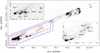 |
Fig. 1 MIRI-MRS map coverage of the HH 211 outflow (Channel 1 in red and Channel 4 in blue). The F460M NIRCam image at 4.6 µm in grey scale is from Ray et al. (2023). The blue circle marks the HH 211 mm position as observed with ALMA by Lee et al. (2019). The zoomed-in inset in the top left corner shows the blueshifted terminal BSs and the inset in the bottom right corner shows the main knots along the blueshifted jet. |
3.2 MIRI-MRS maps: Flow morphology
As mentioned in Sect. 2.1, the MIRI-MRS mosaic covers the whole blueshifted lobe, the central region around the protostar and a small portion of the redshifted lobe (see Fig. 1). NIRCam images show that the collimated blueshifted jet (precessing with a 3.5° opening angle, measured from the NIRCam images) is made of several knots and small BSs (see Fig. 1 and NIRCam image in Fig. 1 of Ray et al. 2023). The blueshifted jet first drives an extended BS (labelled BS 4 in the insets of Fig. 1) and subsequently produces a large terminal BS , which is actually made of three distinct BSs (labelled BS 1, 2 and 3 in the upper-left inset of Fig. 1; BS 1 and BS 3 are also known as knot j - [MRZ94] j - and knot i - [MRZ94] i, respectively, in McCaughrean et al. 1994) with larger precession opening angles (~6°, measured from the NIRCam images).
Figure 3 displays a tricolour image of the H2 0-0 S(7) (5.5 µm), H2 0-0 S(1) (17 µm), and [Fe II] (26 µm) emission lines in blue, green, and red, respectively. Our MIRI maps show that the jet is both atomic and molecular and it is driving a large molecular outflow (see Fig. 3).
The inner jet, within ~2.5″ from the source position (marked by the white circle in Fig. 3), is mostly traced by atomic emission (in red), and the lack of H2 emission is likely due to the large visual extinction (AV >80 mag) close to source. The [Fe II] emission at 26 µm is detected down to ~ 130 and 300 au from the source on the jet red- and blueshifted sides, respectively. Such a difference might be due to different visual extinction or excitation conditions in the two lobes.
The outer jet and BSs show both atomic and molecular emission, whereas the outflow, located at rear and wings of the BSs and likely made of entrained ambient gas, is fully molecular (H2 emission only) and well traced by H2 pure-rotational transitions (in green) at low-energy excitation. Unfortunately, due to the poor MIRI-MRS sensitivity beyond 27 µm, the 0-0 S(0) line is not detected in our maps. The atomic jet is more compact in diameter, whereas the cold H2 molecular component is more extended (see Fig. 3 and Sect. 3.2), indicating a jet onion-like structure with different layers, where the atomic component is at the jet core, nested in a more extended molecular jet (see e. g. Shang et al. 2006; Machida 2014; Shang et al. 2023, and references therein). This structure is readily visible in Fig. A.1 (see Appendix A), which shows a tricolour map of the H2 0-0 S(7) (at 5.5 µm, in blue), [S I] (at 25.2 µm, in green), and [Fe II] (at 26 µm, in red) emission lines. The combination of atomic and hot molecular emission provides a better view of the jet emission. In contrast, the H2 emission (0-0 S(1) line at 17.0 µm) is overplotted with magenta contours. At high S/N (>20), the H2 emission overlaps and cocoons the atomic jet, whereas at lower S/N, it traces a less-collimated wind, as well as BS wings and outflow.
Indeed, the cold H2 component at 17 µm (i.e. the 0-0 S (1) transition - Eup=1015 K, Fig. 3 in green and Fig. 4, bottom panel, and magenta contours of Fig. A.1) is also well detected in the outflow cavity (down to 2″–3″ from the source), likely originating from a less-collimated wind. From the extent of the H2 emission, the half-opening angle of the wind is ≤20º. Curved narrow emission delineates the boundaries of the outflow cavity and the interaction between outflow and ISM. These features become less visible in the H2 transitions at higher excitation energy (e. g., 0-0 S(3) - Eup=2504 K; see middle panel of Fig. 4) and disappear in those at the highest energy (e. g., 0-0 S(7) - Eup=7197 K; see upper panel of Fig. 4).
Notably, no continuum emission is detected on source at the longest JWST wavelengths (26 µm; below 36 MJy sr−1; i. e. Fprotostar (26 µm) ≤0.85 mJy), nor towards the outflow cavities at 5 µm (below 20 MJy sr−1 ). The latter value is about one order of magnitude larger than that of scattered emission (~2.1 MJy sr−1) detected towards the outflow cavities with the NIRCam F460M filter (see Fig. 1). This explains the non-detection in our data. Nevertheless, strong continuum emission longward of 10 µm is observed at BS 1, BS 2, and BS 3, and much fainter emission (S/N~5 σ, longward of 25 µm) along the redshifted jet (Knots 1 and 2 red) and at Knot 4 and, marginally (S/N~3σ), at Knot 3, Knot 2 and BS 4 in the blueshifted jet (see black and white contours in Fig. 3). Towards BS 3, the continuum emission is extended, elongated towards the west (see black contours in Fig. 3), and has a full width at half maximum (FWHM) of ~ 1″.6, which is much larger than that of the nominal point spread function (PSF ~1″) at 25 µm.
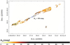 |
Fig. 2 Visual extinction map of the HH 211 outflow derived from the H2 1-0 S(1) and 1-0 O(5) lines (F212N and F323N NIR-Cam images). The colour bar represents the different values in magnitude (mag). A value of AV ≥ 80 mag has been estimated using ro-vibrational diagrams for the source and jet inner regions where the H2 1-0 S(1) emission is not detected. [Fe II] (26 µm) jet contours detected in the MIRI-MRS map are shown in black (see Sect. 3.2). The position of the protostar from ALMA continuum data (see Lee et al. 2019) is also marked. |
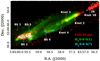 |
Fig. 3 Tricolour MIRI-MRS map of H2 0-0 S(7) (at 5.5 µm, in blue), H2 0-0 S(1) (at 17 µm, in green), and [Fe II] (at 26 µm, in red) emission lines. The white circle marks the position of the ALMA mm continuum source. Black and white contours indicate the position (on the blue- and redshifted lobe side, respectively) of continuum emission integrated between 25.3 and 25.9 µm (displayed contours are at 3, 5, and 50 σ; 1σ=4 MJy sr−1). Knots and bow shocks showing continuum emission are indicated. |
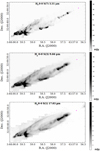 |
Fig. 4 H2 line maps of the brightest transitions detected along the flow. From top to bottom: 0-0 S(7) (5.5 µm), 0-0 S(3) (9.7 µm), and 0-0S (1) (17.0 µm) lines. The magenta circle shows the position of the ALMA mm continuum source. Integrated flux is in mJy pixel−1. |
The jet, the bow shocks, and the outflow
Line maps and spectra indicate that H2 is the brightest and most abundant species along the flow, even along the jet (see top panel of Fig. 5). A large number of H2 transitions (v = 0–0 and v = 1–1, J=1–9, with upper energy levels from ~1000 to 16 000 K) are observed and listed in Table C.1, along with their theoretical wavelength (in µm), energy of the upper level (in K), and corresponding MIRI Channel/Grating.
Another molecule detected along the jet in the MIRI-MRS data is HD (see spectrum in Fig. 5 and top panel of Fig. A.2). Several faint 0-0 R transitions (see Table C.3) are detected both along the blueshifted jet and in the outer BSs. HD emission is analysed in detail in a forthcoming paper (Francis et al. in prep.). CO2 at 15 µm is also faintly detected (S/N~3σ) in Knot 2 (see Fig. 5 and TableC.5).
In addition to the molecular emission, several atomic species are detected along the jet. Besides the many transitions of [Fe II] with the excitation energy of the upper level (Eup) ranging from ~500 to ~4000K (see Fig. 5 and TableC.2), strong [S I] and [Fe I] emission (see middle and bottom panels of Fig. 6) at 25.25 and 24.04 µm, respectively, are detected. We note that these transitions have Eup similar to the [Fe II] line at 26 µm (~550– 600 K). These features match the jet very well, delineated by the [Fe II] emission (see the top panel of Fig. 6), although the intensity of such lines largely vary along the flow, and likely follow the different excitation conditions along the jet. Indeed, the continuum-subtracted map in Fig. 6 show that [Fe I] emission, seen for the first time in a protostellar jet, is mostly detected along the jet, whereas faint (S/N≤5) or no emission is seen at the outer BSs, where [Fe II] and [S I] emission lines are strongest. This almost certainly reflects an increase in the ionisation fraction along the flow. The other atomic species detected along the jet is [Ni II] at 6.6 µm (see Fig. A.2). Two more transitions from [Ni II] are also observed at BS 3 (see Table C.2).
The terminal BSs (BS 1–BS 3) are clearly richer in terms of chemistry, especially BS 3, which is the brightest (see Fig. 7). In addition to the species visible along the jet, many other molecular and atomic forbidden lines are detected (see Tables C.2 and C.3). In particular, the tail (i.e. J ≥25 up to J=59) of the P-branch CO fundamental (i. e. v = 1 – 0, up to ~5.4 µm) is the brightest molecular emission after H2 (see Fig. 7, and middle upper panel of Fig. A.2), although P- and R-branch low-J lines at shorter wavelengths (i. e. between ~4.4 and ~5 µm) are brighter (their total flux is ~4–5 times larger than that from the tail; see HH 211 BS 1 NIRSpec spectrum in Fig. 2 of Ray et al. 2023). Our MIRI-MRS spectra only show CO on the four BSs (BS 1–BS 4, see Fig. A.2, middle panel), but not along the jet or the outflow (see NIRCam image in Fig. 4 of Ray et al. 2023), since the integrated CO emission in the NIRCam image of Ray et al. (2023) is about one order of magnitude fainter than our map 3σ threshold sensitivity (~0.4 mJy arcsec−2 or ~17 MJy sr−1).
Plenty of OH lines (between 9.1 and 25 µm) are detected in the spectra of the terminal BSs (see Fig. 7), coming from pure rotational states (v = 0, J′ → J′−1) arising in the 2Π3/2 and 2Π1/2 ladders and cross-ladder. These OH MIR lines (suprathermal OH rotational emissions; see Neufeld et al. 2024) originate from water photodissociation by 114–143 nm UV radiation, produced in this case by strong jet shocks (v ≥ 40 km s−1) (see, e g. Tabone et al. 2021; Zannese et al. 2024). This emission was already observed in low-resolution Spitzer/InfraRed Spectrograph (IRS) spectra of HH 211 (see Tappe et al. 2008) and also predicted and modelled by Tabone et al. (2021). In addition, these MIR lines were also observed with Spitzer in DGTau (at λ > 13 µm Carr & Najita 2014) and recently detected with MIRI also in the HOPS 370 jet (see Neufeld et al. 2024). Additional H2O transitions (v = 0 − 0 and v2 = 1 − 0), as well as faint HCO+ (v2 = 1 − 0) at 12 µm and CO2 at 15 µm are also detected in the spectra of the three outer BSs (see Fig. 7).
Other atomic forbidden lines in emission detected in BS 3 include bright [Cl I] at 11.3 µm (also detected in BS 1 and 2, see Fig. A.2), [Ne II] at 12.8 µm, barely visible in BS 1, as well as faint (S/N≤3σ) emission of [Ar II], [Cl II], [Co II], and [S III] (see Fig. 7 and TableC.2). Notably, all these atomic lines and their intensities were predicted in Hollenbach & McKee (1989, hereafter, HM89) J-shock models.
3.3 Jet radius
A noteworthy result from our line maps is that the size of the inner jet is resolved, or marginally resolved, in both atomic species ([Fe II] at 26 and 17.9 µm, [Fe I] , and [S I] ) and H2 lines (0-0S(7) and 0-0S(1)). We compute the diameter of the jet for the different lines for various knots (knot id. and coordinates are listed in Table 1), measuring the FWHM orthogonal to the jet axis at each knot position, after collapsing the image over the knot size along the jet axis. The spatial line-profile is then fitted with a 1D Gaussian and the resulting deconvolved diameter (or jet size) is  , where PSF is the point-spread function value at wavelengths close to those of the emission line. For the atomic lines and the H2 0-0 S(1) line, we measure the PSF of the continuum emission towards BS 1, which is not spatially resolved. As no continuum is detected at 5.5 µm, to infer a reference PSF for the H2 0-0 S(7) line we use a set of faint H2O lines towards BS 1, which do not seem to be spatially resolved. The obtained value is 0″.3, which is similar to the nominal one reported in Law et al. (2023) (0″.28). It is also worth noting that, as the H2 jet is fully resolved (0″.5–1″) at this wavelength, a difference of 0″.02 would not significantly affect its inferred size.
Measured FWHMs (in″), deconvolved sizes (in″) and radii (in au) of the jet for the different species and at different positions are reported in Table C.4. Figure 8 shows that the jet radius varies for the different species (i.e. [S I], [Fe II] 26 µm, H2 0-0S(1) and S(7) lines, depicted as green dots, magenta triangles, blue, and black triangles, respectively) at different distances from the source. The position and name of each knot are labelled in red at the bottom of the figure.
Overall, Fig. 8 confirms the onion-like structure of the jet, with the atomic jet displaying smaller radii and the molecular component larger radii. The different atomic lines show similar values in radius (ranging from ~45 to ~100 au), possibly because the angular resolution is not sufficient to separate neutral and ionised gas. On the other hand, the H2 lines have radii similar or larger than the atomic jet. The radius of the H2 0-0 S(7) line ranges from ~60 to ~130au, whereas the 0-0 S(1) line is positioned on the outer layers of the jet (~ 100–180 au).
In most cases, the jet size is just marginally resolved (see Table C.4). Therefore, these trends can hardly be seen in our maps, with the exception of the H2 0-0S(1) emission line, which overlaps and encloses both atomic and hot H2 molecular emission (see Figs. 3 and A.1).
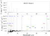 |
Fig. 5 Spectrum of the HH 211 blueshifted jet extracted at Knot 2 (RA(J2000): 03h43m57s.331, Dec(J2000): +32°00′47″.04). The top panel shows the full flux-density range of the spectrum (up to 2.5 × 10⁻¹¹ erg s−1 cm−2 µm−1), and the bottom panel shows a close-up (up to 6.5 × 10⁻¹³ erg s−1 cm−2 µm−1). Detected lines are labelled. Different colours indicate different species. |
ne and Te values from [Fe II] analysis along the HH 211 flow.
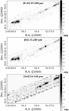 |
Fig. 6 [Fe II] (26 µm), [S I] (25 µm), and [Fe I] (24 µm) continuum-subtracted emission lines along the jet (from top to bottom in the panels). The magenta circle shows the position of the ALMA mm continuum source. Integrated flux is in mJy pixel−1. |
3.4 H2 ro-vibrational diagrams
The large number of H2 rotational transitions from v = 0 and v = 1 levels and their ample range of excitation energies (1000 K ≲ Eup ≲ 16 000 K) allow us to infer both gas temperature (T(H2)) and column density (N(H2)) along the flow (see e.g. Giannini et al. 2004; Caratti o Garatti et al. 2006) by means of ro-vibrational diagrams. Extinction-corrected line column densities, divided by their statistical weights, are plotted against their excitation energies using a semi-logarithmic scale. For a gas in local thermal equilibrium (LTE), the gas excitation follows a Boltzmann distribution (Nv,J/ɡv,J ∝ exp(−Ej/kTex)) and points in the diagram align in a straight line, whose slope is the reciprocal of the gas excitation temperature (if Tex=Tgas). The y-axis intercept provides the gas column density. Often, the H2 gas shows stratification in temperature. Generally, transitions at low excitation (Eup ≲4000–5000 K) trace a cold component (T(H2) ≲1000 K), those at higher energy (Eup ≲ 10 000–12 000 K) a warm component (T(H2) <2000–2500 K), and those at the highest energy a hot component (T(H2) ~ 3000–4000 K).
Lines tracing the cold, warm, and hot components can be detected at MIR wavelengths (see Table C.1). Therefore, the MIRI-MRS regime can trace up to three H2 components, and we might expect to measure up to three different temperatures and column densities (see e.g. Neufeld et al. 2009; Dionatos et al. 2010), with the cold component tracing the highest column densities and the hot component the lowest.
Unfortunately, it is not possible to directly measure the visual extinction with our MIRI-MRS data, as we do not detect any pair of H2 transitions arising from the same upper level in the MIRI wavelength range. However, a rough estimate (usually within a 5–10 mag uncertainty) can be also inferred by varying AV in the ro-vibrational diagrams and maximising the correlation coefficient in the fits of the Boltzmann plots. We use this technique to infer the visual extinction of the inner jet region of HH 211 (namely Knot 1, 1R, and 2R), too embedded to be detected in the 1−0 S(1) NIRCam filter (see Fig. 2). The ro-vibrational diagram shows that the blue jet closest to source has an AV value of 80 mag (see Fig. B.1) and we thus adopt this visual extinction value within an ~6″ (~ 1930 au) radius from the source, namely where no meaningful extinction value is measured in our AV map (see Fig. 2). It is worth noting, however, that close to the source (i.e. within 2″–3″ from the source, where no H2 emission is detected) and on-source the visual extinction is very likely much higher that 80 mag (probably AV > 100mag; as hinted by the lack of continuum MIR emission on source at λ ≤ 27 µm, see Sect. 3.2, as well as the disappearing of the [Fe II] atomic jet close to the source).
To measure the H2 excitation conditions, we employ a pixel-by-pixel ro-vibrational diagram analysis as described in Gieser et al. (2023). Briefly, the python routine first provides sub-cubes around the H2 lines of interest (see Table C.1) and resamples each sub-cube to a common (and worst) spatial resolution of 0″.7 (0″.2 pixel-scale size) of MIRI-MRS Channel 3. Each sub-cube is then dereddened using the AV map presented in Appendix B.
Line fluxes are derived for each line by extracting the spectrum from each spaxel of the corresponding sub-cube and by fitting a 1D Gaussian profile, as the H2 lines are barely spectrally resolved with MIRI-MRS. To avoid spurious detection, a flux threshold of 40 MJy sr−1 per spaxel is set in the original cube. As a further constraint, fits to the ro-vibrational diagrams are done only if five or more transitions are detected in a spaxel. Ro-vibrational analysis is performed using the pdrtpy1 Python package.
In our ro-vibrational plots we detect a mixture of temperatures. The prdtpy package was set to fit two components in our diagrams. For simplicity, we call them warm and hot components, following the nomenclature of Gieser et al. (2023). This is to distinguish the warm H2 gas from the colder outflow traced by other species at sub-mm wavelengths. However, it is worth noting that both temperature and column of each component largely vary along the flow, depending on the gas excitation conditions, that is on the number of detected lines and their excitation energies (see examples in Fig. B.2 of Appendix 3.4). Therefore our simplification is highly reductive.
Figure 9 shows temperature (top panels) and column density (bottom panels) maps for the warm (left panels) and hot components (right panels) of the gas. Overall, the gas is colder and denser in the inner jet, whereas it becomes warmer and less dense in the outer BSs. Moreover, the warm component has column densities one order of magnitude larger than the hot component (see bottom panels of Fig. 9).
The temperature of the warm component varies from ~300 K, in the inner jet close to source, to 500–700 K along the jet, and up to 900–1000 K in the terminal BSs, and its column density changes from 1019 to 1020 cm−2 along the jet, while it is just some 1019 cm−2 along the BSs, with the exception of BS 3, which has the highest column densities (~3 × 1020 cm−2).
The hot component varies from 1000 to 2000 K along the jet, whereas it is much higher (2000–3500 K) at the BSs. On the other hand, its column density is higher along the jet (1–2 × 1019 cm−2) and drops in the outer jet and BSs (1018– 1019 cm−2).
Less collimated, colder (200–400 K) and less dense (1018– 1019 cm−2) gas (showing a U or V shape at the rear of the jet) is detected in the inner regions (bottom panel of Fig. 4 and left panels of Fig. 9), likely tracing a poorly collimated wind. In addition, the outflow gas (i. e. the entrained gas) appears less dense and colder than that in the jet and BSs, with the exception of the shocked outflow-ISM interface (blue coded in the N(H2) maps), where column density and temperature appear to be higher than those of the entrained gas.
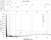 |
Fig. 7 Spectrum of HH211 BS3 (see Fig. 1) extracted at RA(J2000): 03h43m59s.413, Dec(J2000): +32°00′35″.27. The top panel shows the Ml flux-density range of the spectrum (up to 7 × 10- erg s−11 cm−2 µm−1), and the bottom panel shows a close-up (up to 10−12 erg s−1 cm−2 µm−1). Detected lines are labelled. Different colours indicate different species. |
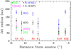 |
Fig. 8 Inferred jet radius (in au) vs. distance (in arcseconds) from the source for different lines. Green dots, magenta triangles, and blue and black triangles show [S I], [Fe I] (at 26 µm), H2 0-0 S(1), and S(7) lines, respectively. Knot identification is displayed in red. |
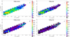 |
Fig. 9 Temperature (top panels) and column-density (bottom panels) maps of the warm (left panels) and hot (right panels) H2 components. The magenta circle shows the position of the ALMA mm continuum source. |
3.5 Physical properties of the flow from the atomic species
We can use the different atomic species detected along the flow to infer the main physical parameters of the atomic gas.
3.5.1 Electron density and temperature from [Fe II]
Electron density (ne) and temperature (Te) of the atomic gas can be derived from the many [Fe II] transitions detected along the flow in the MIRI-MRS data. For our analysis, we use a nonlocal thermal equilibrium (NLTE) excitation model presented in Giannini et al. (2013), here updated to include the MIRI-MRS transitions at low Eup. The model assumes electronic collisional excitation/de-excitation and spontaneous radiative decay. It employs the atomic database of the XSTAR tool (Bautista & Kallman 2001), which provides energy levels, Einstein coefficients, and collision rates (for temperatures between 2000 K and 20 000 K) for the first 159 fine-structure levels of Fe+. Our NLTE model provides a line intensity grid for all transitions from the 159 levels for 100 ≤ ne ≤ 107 cm−3 (in steps of log10 (δne/cm−3) = 0.06) and 400 ≤ Te≤ 105 K (in steps of δTe=200 K).
The observed line fluxes are de-reddened using the values reported in our AV map (see Sect. 3.1), and their line ratios are used to find the best fit to our model, leaving Te and ne as free parameters. Fits with the lowest chi-square (χ2) value provide the best Te and ne solutions.
Along the jet we just detect the [Fe II] lines at 5.3, 17.9, and 26 µm. On the other hand, for the external BSs more lines have been used in our fits (see Column 6 of Table C.2).
Spectra with 1″ radii were extracted from eleven regions, the four outer BSs (BS 1–4), five knots along the blueshifted (Knot 1–5), and redshifted jet (Knot 1 red and 2 red) (see Fig. 1 and Column 2 of Table 1 for feature identification and coordinates, respectively). Only in seven of these spectra (i. e. the four BSs and Knot 2, 3, and 5) the [Fe II] 5.3 µm line is bright enough for our analysis (≥5σ).
Columns 3 and 4 of Table 1 report ne and Te values of the fits for each feature, while Column 5 lists the χ2 of the best fit along with its degrees of freedom (i. e. number of line ratios used minus the two variables, ne and Te). Temperature increases moving away from the source, notably from Te ~1000 K in the inner jet to Te ~ 1400K in BS4, Te ~2800 K moving further out to Knot 5, and it reaches its peak at BS 3 (Te ~3800 K). Te finally drops in the two most external BSs, BS 2 and BS 1, at 1800 and 2400 K, respectively. The trend of ne is similar, low values (100–230 cm−3) along the jet and at BS 4 and higher values (350–800 cm−3) at the three terminal BSs (BS 1–BS 3).
It is also worth noting that the three brightest [Fe II] lines (i. e. at 5.3, 17.9, and 26 µm) can be combined to infer both parameters, as the 17.9/5.3 µm ratio is sensitive to ne and the 26/17.9 µm ratio to Te. Figure 10 shows a plot of the two line ratios (26 µm/17.9 µm line on the x-axis and 17.9 µm/5.3 µm line ratio on the (y-axis) in logarithmic scale and the grid of Te and ne values derived from our model. Line ratios and uncertainties of each analysed feature are displayed (BSs in blue, knots in red). Derived values and errors for ne and Te are listed in Columns 6 and 7 of Table 1, respectively. Within the error bars, these results are the same as for the fits; however these numbers provide a better constraint on the uncertainties. The larger uncertainties are those on ne along the inner jet and this is due to the fact that the 5.3 µm line has a relatively low S/N (≤5) there. For four more knots (Knot 1 and Knot 4 blueshifted, and Knot 1 and Knot 2 red-shifted, the latter labelled with an additional R for distinguishing purposes in Fig. 10 and other figures and tables of the paper), we report lower limits on ne (as the 5.3 µm line is not detected or is below 3σ in our spectra) and the corresponding temperature upper limits. The upper limit to the 5.3 µm line flux is inferred by multiplying the 3σ noise of the spectrum at the line wavelength by the nominal FWHM of the line.
Finally, we employ continuum-subtracted line images of the three bright [Fe II] lines to construct both log (26 µm/17.9 µm) and log (17.9 µm/5.3 µm) maps, to visualise how Te and ne vary along the flow. Images were sampled at the lowest pixel scale of the 26 µm image, and, to avoid spurious detection, pixels with fluxes below 3σ were masked. Furthermore, in the resulting maps, only pixels within the 3σ line contours are displayed.
Figure 11 shows the logarithmic map of the 26 µm/17.9 µm line ratio. The colour-coded bar reports both logarithmic values and the corresponding Te for a gas with ne=500 cm−3 (i. e. an average of the measured range of values along the flow). Therefore, the corresponding temperature is slightly underestimated along the jet and overestimated along the terminal BSs. Notably, the counter-jet has Te similar to the jet and the increasing Te trend towards the terminal shocks is also visible. Figure 12 shows the logarithmic map of the 17.9 µm/5.3 µm. The colour-coded bar indicates the corresponding ne of a gas at Te=1000 K. Electron densities are lower along the jet and in BS 4 whereas they are higher in the outer BSs.
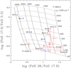 |
Fig. 10 Logarithmic grid of the [Fe II] 26 µm/17.9 µm line ratio (x-axis) and [Fe II] 17.9 µm/5.3 µm line ratio (y-axis). The two line ratios are sensitive to Te and ne, respectively. Line ratios and error bars for the studied features (BSs in blue, knots in red) are shown in the plot. |
3.5.2 Gas-phase iron abundance
Gas-phase iron abundance, and thus the observed [Fe II] and [Fe I] line intensities, are regulated by the shock efficiency in eroding the dust grains, through processes like sputtering and grain-grain collision, which release iron into the gas-phase (see, e. g. Seab 1987; Jones 2000; Colangeli et al. 2003). Studies of nearby protostellar jets at near- and MIR wavelengths have shown that the gas-phase abundance of Fe is much lower than the typical solar abundance (i. e. (Fe/H)⊙=2.88 × 10−5; see, Asplund et al. 2021), indicating that, if solar abundance is assumed, metals are still partially locked onto grains (see, e. g., Nisini et al. 2002; Podio et al. 2009; Dionatos et al. 2009, 2010). Typically, this type of analysis is conducted by comparing [Fe II] line intensities with those from a non-refractory species (e. g., Ne, S, O, P, Cl) emitted under the same physical conditions and assuming solar abundances.
An analysis of Fe and Si gas-phase depletion in HH 211 was accomplished by Dionatos et al. (2010) with Spitzer/IRS, using sulphur as a non-refractory species. They found a gas-phase Fe abundance between 3–10% and 2–7% with respect to the solar one for the blue- and redshifted jet, respectively (see their Table 5). However, as no [Fe I] emission was detected in their spectra, they assumed that the iron was fully ionised, and therefore those values should be considered as an upper limit of the iron abundance (or a lower limit value of the Fe gas-phase depletion) along the flow.
Constraints on the gas-phase iron abundance can be also inferred by comparing observed dereddened line ratios with those predicted in dissociative shock models (see, e. g., Nisini et al. 2002). To trace the iron abundance, we use the observed [Fe II] 26 µm/[S I] and [Fe I]/[S I] line ratios, as both [Fe I] and [Fe II] lines are equally depleted along the jet. We assume solar abundance for the different species and, most importantly, that S is a non-refractory species, and thus it is all in the gas phase. It is worth noting, however, that the latest studies in nearby molecular clouds have shown that sulphur is a semi-refractory species, and its depletion depends on the environment and star formation activity (see e.g. Fuente et al. 2023). In particular, Fuente et al. (2023) show that S is, on average, depleted by a factor of 20 in the Perseus molecular clouds.
For different knots along the jet, we compare the observed line ratios against those predicted by HM89 J-shock models for different values of the gas-phase iron abundance and a range of shock velocities (vs=30–100 km s−1).
Figure 13 shows the observed line ratios for different knots (red triangles) plotted over the HM89 original values (black open circles), calculated for H I pre-shock density of n0=105 cm−3 and an Fe abundance of 10−6. Predicted [S I] line fluxes have been modified to take into account the slightly different S abundance in the original HM89 model (10−5) with respect its most recent solar abundance (1.318 × 10⁻⁵; Asplund et al. 2021). The same curve is plotted for a range of gas-phase iron abundances (plotted in different colours, as labelled in the figure): from solar (2.88 × 10⁻⁵, black dots curve, upper right) to 7 × 10⁻⁷ (magenta open circles curve, lower left). Changes in pre-shock density moves the curves as shown by the blue arrows in the plot.
Figure 13 shows that Fe is largely depleted (i. e. knots fall far away from the curve with solar abundance - black dots curve) and just a small amount is in gas-phase (between ~2 and ~10%), as abundances range from ~7 × 10⁻⁷ to ~3 × 10⁻⁶. Knots close to the source (namely Knot 1, Knot 1 red and 2 red) seem to be less depleted than those positioned further away from the source (i.e. Knots 2, 3, and 4). Although we cannot be certain about the absolute values of Fe depletion, which rely on the assumption that S is not depleted, we can be confident regarding the Fe differential depletion along the jet.
Nevertheless, one would expect the opposite of what we find, namely that the Fe gas-phase increases along the flow moving away from the source (see e.g. Nisini et al. 2005; Podio et al. 2006), as Fe is being released from grains via shocks along the flow. Our measure of a decrement in the Fe gas-phase along the jet (see Fig. 13) suggests that this difference is local and related to the different strength of the shocks along the flow, rather than a continuous destruction of grains along the flow.
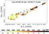 |
Fig. 11 Logarithmic map of the ratio of [Fe II] lines at 26 µm and 17.9 µm. Cyan contours show the [Fe II] (26 µm) line flux at 3, 10, and 50 σ (0.48, 1.6, 8mJy pixel−1). Colour code displays the logarithmic value of the ratio (bottom) and the corresponding Te (in Kelvin) for an average ne of 500 cm−3. Only pixels within 3σ line contours are displayed. The magenta dot shows the position of the ALMA mm continuum source. |
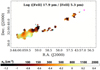 |
Fig. 12 Logarithmic map of the ratio of [Fe II] lines at 17.9 and 5.3 µm. Cyan contours show the [FeII] (5.3 µm) line flux at 3, 10, and 50σ (0.1, 0.4, 2.1 mJy pixel−1). Colour code reports the logarithmic value of the ratio (bottom) and the corresponding ne (in cm−3) for an average Te of 1000 K. Only pixels within 3σ line contours are displayed. The magenta dot shows the position of the ALMA mm continuum source. |
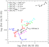 |
Fig. 13 Observed vs. predicted [Fe II] 26 µm/[S I] and [Fe I]/[S I] line ratios for different knots (red triangles) along the jet. Each curve reproduces the Hollenbach & McKee (1989) dissociative models for different values of the gas-phase iron abundance (coloured curves, from 2.88 × 10⁻⁵ – black dots – to 7 × 10⁻⁷ – magenta open circles), pre-shock density n0=105 cm−3, and a range of shock velocities (vs=30–100 km s−1), as reported in the labels. The two blue arrows show how the plots move by varying n0 from 104 to 106 cm−3. |
3.5.3 Density, shock-velocity, and ionisation fraction of the atomic jet
Figure 13 already provides us with some indications about pre-shock densities (n0) and shock velocities (vs) along the flow. However, as both iron abundance and ionisation fraction are not well constrained by such analysis, it is not possible to properly infer vs and n0 values. The latter parameter is particularly important to define the dynamical properties of the atomic jet component and thus its relevance with respect to the molecular component.
We can use other atomic lines predicted by the HM89 models, to constrain these two parameters. In particular, we note that the [Ne II] line intensity strongly depends on vs, but it is less sensitive to n0 variations (see Fig. 7 in HM89). In contrast, [S I] and [Cl I] (at 11.4 µm) line intensities are strongly dependent on n0 variations but not on vs (at least for shock velocities ≲60 km s−1).
Therefore, we first constrain the shock velocity along the flow using the dereddened [Ne II] line intensity as observed in different BSs and knots of HH 211. As the line is detected below 3σ (or not detected) in the knots along the jet, here we use a 3σ upper limit to estimate its line intensity. Shock velocities of 40±5 km s−1 are measured for the BSs (35±5 km s−1 for BS 2), whereas vs < 50–60 km s−1 is inferred along the jet. Results are listed in Column 2 of Table 2.
We then employ [S I] and [Cl I] line fluxes to infer the gas pre-shock density. Values derived from [S I] are more reliable, as [Cl I] is only weakly detected along the jet (S/N≤3σ). Despite this, n0 values derived from [Cl I] are consistent with those derived from [S I] (see Column 3 of Table 2).
Pre-shock density along the jet ranges from 7 × 10⁴ to 2 × 105 cm−3, being denser (1–2 × 105 cm−3) in knots close to the source (i.e. Knot 1, Knot 1 red and 2 red). The outer jet and BSs show a lower density (4–9 × 104 cm−3).
By combining ne and n0, it is then possible to infer the H I ionisation fraction (xe=ne/n0). Values along the jet are a few 10−3 (see Column 4 of Table 2), whereas at the terminal BSs it is slightly higher (from several 10−3–10−2). We note that these values are similar to what was inferred in HH 211 with Spitzer by Dionatos et al. (2010). Such small xe values are typical of Class 0 protostellar jets (see e.g. Dionatos et al. 2009, 2010), in contrast to Class I and II jets, where xe ranges from 0.03 to 0.9 (see e.g. Ray et al. 2007; Frank et al. 2014, and references therein).
Physical and dynamical parameters along the HH 211 atomic flow.
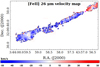 |
Fig. 14 [Fe II] 26 µm radial-velocity map. Black contours show the integrated continuum-subtracted line intensity at 5σ (0.8 mJy pixel−1). The magenta dot shows the position of the ALMA mm continuum source. |
3.6 Flow kinematics
MIRI-MRS datacubes also allow us to explore the velocity structure along the flow for the brightest atomic ([Fe II], [S I], [Fe I]) and molecular (H2) lines. To derive radial velocity maps of these lines, we employ the python routine bettermoments (Teague & Foreman-Mackey 2018) and fit a Gaussian line profile to each pixel with a S/N≥5σ in each line image. Depending on the S/N of the spectral line, this method typically provides a radial velocity precision ( , where Δvr = c/R) much higher than the nominal spectral resolution (R) of the instrument.
Radial velocity maps for [Fe II] at 26 µm (see Fig. 14) and 17.9 µm, [S I], [Fe I] (see Fig. D.1), and H2 0-0 S(1) and S(7) (see Fig. D.2) lines were constructed.
Figure 14 shows the radial-velocity (vr) map of the [Fe II] at 26 µm. The red and blue lobes of the jet are detected straddling the protostar’s position as derived by ALMA (magenta circle; see Lee et al. 2019). Radial velocities have an average value of vr= −25±5 and +25±5 km s−1 in the blue and redshifted inner jet respectively (see Column 2 in Table C.6). These values translate to a total velocity (vtot) of about 130±25 km s−1, assuming a jet inclination angle (i) of 11° with respect the plane of the sky, as derived from the SiO analysis (see Jhan & Lee 2021). At ~20″ from the source radial velocity values increase up to approximately −30±5 km s−1 (i.e. vtot=160±25 km s−1, assuming that i is constant along the jet. As the jet shocks the ambient medium forming BS 4, vr drops to approximately −20 km s−1.
Indeed, the terminal BSs have lower velocities, which might be real or just caused by slightly different jet inclination angles; vr(BS1)=−20±5 km s−1, vr(BS2)=−15±5 km s−1, and, at BS 3, the radial velocity becomes slightly redshifted (vr=5±5 km s−1 km s−1), possibly indicating that the direction of the flow has changed and the inclination with respect to the observer is larger than 90° (see Column 2 in Table C.6).
We note that the position of such redshifted emission is slightly offset with respect of BS 3, namely ~1″ north of the BS 3 peak. We also note a similar redshifted radial velocity in the [Fe II] 17.9 µm velocity map at the same position (see bottom panel of Fig. D.1). However, both [S I] (upper panel of Fig. D.1) and H2 (Fig. D.2) velocity maps do not show any redshifted emission at this location ([Fe I] emission at BS 3 is below 5σ), indicating a different geometry for those species or a different origin for the [Fe II] redshifted emission. This might otherwise suggest the presence of a second, independent flow, traced by the [Fe II] in the BS 3 region, as a N-S crossing flow was possibly detected in the NIRCam images of Ray et al. (2023).
Overall, both [S I] and [Fe I] velocity maps show, within the uncertainties, radial velocities similar to those in the [Fe II] maps (see Figs. D.1 and 14). The H2 lines (see Fig. D.2) have a similar behaviour, but show radial velocities ~10 km s−1 lower than the atomic species (see Column2 and 3 of Table C.7). Overall, gas traced by the H2 0-0 S(1) line moves at slightly lower speed than that traced by the 0-0 S(7) line (see Columns 2 and 3 of Table C.7). Jet radial velocities of the 0-0 S(7) line range between ~14 and ~20 km s−1 (but the same velocity within the error bar) and then vr drops to ~8–12 km s−1 at the terminal BSs. On the other hand, the molecular outflow shows radial velocities lower than the molecular jet (see Fig. D.2), ranging from −10 to −3±5 km s−1, and the poorly collimated (wind) emission close to source has radial velocities ≤−5 km s−1 (see Fig. D.2).
Assuming that the H2 0-0 S(7) line (Eup=7197 K) is tracing the same gas and velocities as the 1-0 S(1) line (Eup=6956 K), we can derive the flow inclination at different positions by combining the tangential velocities (vtg), measured in Ray et al. (2023) (reported in Column 4 of Table C.7), and the radial velocities measured here. The inclination angle with respect to the plane of the sky ranges from 9°.8±1°.5 to 12°±1° along the jet (Column 7 of Table C.7), and the weighted mean is 11°.6±0°.6, which perfectly matches the inclination value from SiO (Jhan & Lee 2021), confirming that our previous assumption on i was correct. On the other hand, the terminal BSs have a much larger spread in i, ranging from 5°.5±4°.4 to 19°.4±2°.1 (see BS 1 to 4 in Column 7 of Table C.7). These differences are not unexpected, as they reflect the larger precession angle measured in the outer BSs (see Sect. 3.2).
We can also infer the total velocity of each feature for the 0-0 S(7) line from both inclination and 1-0 S(1) tangential velocities (Column 5 of Table C.7). For those knots where no vtg nor i are available, vr and an average value of i=11º are assumed. The corresponding uncertainties are therefore larger. Similarly, we compute total velocities for the 0-0 S(1) line (Column 4 of Table C.7). Given the small inclination of the flow, within the uncertainties, vtot of the H2 0-0 S(7) line is the same as vtg inferred in Ray et al. (2023) (see Columns 5 and 4 ofTableC.7). Total velocities inferred from the 0-0 S(1) line are similar or slightly smaller than those inferred for the H2 0-0S(7) line (see Columns 6 and 5 of Table C.7).
An interesting feature, detected in the atomic species ([Fe II] at 26 µm, [S I], and [Fe I] ) along the inner jet (within ~10″ from the source position) is a a mirror symmetry in radial velocities between the two sides of both blue- and redshifted jet (see Figs. 14 and D.1). The bottom side (towards SE) of the blueshifted jet has an average vr of −40 ± 10 km s−1, whereas the top side (towards NW) has vr of −15± 10 km s−1. Conversely, the top side (NW) of the redshifted jet has vr~40±10 km s−1 and bottom side (SE) of 15± 10 km s−1. Although the differences are per-se small (Δvr=25±15 km s−1) and almost within the uncertainties, they may well be significant because they are detected in all the three maps and the shifts in the red- and blueshifted lobes are reversed. One possible explanation is that we are detecting jet rotation (counterclockwise, i.e. the bottom side is approaching and the top is receding) from a few hundred to a several thousand au from the source. Alternatively, jet precession (Cerqueira et al. 2006), asymmetrical jet shocks (De Colle et al. 2016), or the, less likely, presence of a twin jet (e. g. Soker et al. 2022) could also explain the observed shifts. We note a similar velocity gradient (1.5±0.8 km s−1 at 30 ± 15 au from the jet axis) was detected by Lee et al. (2007) in SiO with the SMA. However, ALMA observations at similar resolution, but with higher sensitivity, in Lee et al. (2018) could not find any clear rotation signal and instead found only an upper limit of ~27 au km s−1 for the inferred jet specific angular-momentum. This upper limit is more than one order of magnitude smaller than what was found here, making it very unlikely we are detecting jet rotation.
H2 column densities and mass flow along the HH 211 flow for the warm (W) and hot (H) components.
3.7 Molecular and atomic mass-flux rates along the jet
Using both physical and kinematic parameters derived from the H2 and atomic lines, mass ejection rates along the jet can be inferred.
For the warm and hot H2 components we assume that the jet has laminar flow across the observed pixels in each considered knot along the blueshifted jet (see, e. g., Dionatos et al. 2010):
 (1)
(1)
where µ (=1.35) is the mean atomic weight, mH is the proton mass,  is the H2 column density (warm and hot, see Column 3 and 4 in Table 3, respectively) averaged over the knot emitting area (A; assumed circular and derived from the radii reported in Table C.4), vtg is the knot tangential velocity (see Table C.7) and ltɡ (see Column 2 of Table 3) is the measured knot cross section. Only values for knots along the blueshifted jet are reported, as the H2 column densities are poorly constrained in the redshifted jet (see Fig. 9).
Mass-flux rates for the warm and hot H2 components are reported in Column 5 and 6 of Table 3, respectively. Derived  range from 5 to 8 × 10⁻⁷ M⊙ yr−1, whereas
  are about one order of magnitude smaller, given the lower column density and (typically) smaller emitting size of the hot component. Overall, our mass flux rates are typically two or three times smaller than those found by Dionatos et al. (2010) with Spitzer, likely due to the poor spatial resolution of the Spitzer/IRS modules, whereas both column densities and velocities are similar. No mass-loss rates are derived for the external BSs, because they would likely be overestimated, as part of the observed material is made of entrained gas from the ISM.
Assuming that both blue- and redshifted jet are symmetric (i. e. redshifted knots have same mass-flux), we infer a mass-ejection rate along the jet of Ṁjet(H2)=1−1.6 × 10⁻⁶ M⊙ yr−1. These values perfectly match those derived from the SiO and CO jet by Jhan & Lee (2021) (1.1 × 10⁻⁶ M⊙ yr−1 with v = 100 km s−1) and Lee et al. (2010) (1.8 × 10⁻⁶ M⊙ yr−1 with v =170 km s−1). Using the mass accretion rate inferred by Lee et al. (2010) from Lbol (Ṁacc=8.5 × 10⁻⁶), Ṁjet/Ṁacc varies from 12 to 19%, consistently with what was found with ALMA. Such a high Ṁjet/Ṁacc efficiency is predicted by MHD disc-winds at the protostellar stage (see, e. g., Ferreira et al. 2006).
As column density, mass flux, and velocities are known, other important dynamical properties of the flow can be retrieved. In particular, momentum (P = M × vtot) and momentum flux (Ṗ = Ṁ × vtot) of the molecular component can be inferred and compared with those of the atomic component, to examine whether the molecular jet is made of entrained material or it belongs to the jet, being launched from the disc.
Columns 7–9 of Table 3 report momentum, momentum flux, and dynamical time (τ) for the warm H2 component of the analysed knots.
To compare molecular and atomic dynamics, the mass-loss rates of the various knots (Ṁknot) were derived from the physical and kinematic parameters inferred in Sects. 3.5.3 and 3.6. Ṁknot can be expressed in terms of the pre-shock density (n0), speed of the gas entering the shock, and jet radius (rj, as inferred in Table C.4):
 (2)
(2)
As n0 was obtained from [S I], rj values are also taken from [S I] in Table C.4. In any event, this assumption should not change our results as [S I] and [Fe II] have the same rj values within the error bars (see also Fig. 8).
The average jet velocity is assumed to be vtot=130 ± 25 km s−1 (see also Sect. 3.6)2. Namely, as [S I] and [Fe II] radial velocities are similar, knot radial velocities from Table C.6 are converted to velocities assuming a jet average inclination angle of 11°.
As in the case of H2, Ṁ, P, Ṗ, and τ (Columns 5–8 of Table 3, respectively) are computed for the atomic component. Ṁ, P, and Ṗ values of the atomic (red dots) and warm H2 component (black dots) components of each knot are plotted in Fig. 15 (bottom, middle, and top panel, respectively) as a function of the distance to the source. It is clear that the dynamical parameters of the atomic jet are always smaller than those of the warm H2 component (H2(W)), indicating that most of the thrust of jet derives from its molecular component. Most importantly, this confirms that the molecular jet is not entrained but originates from the disc.
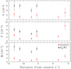 |
Fig. 15 Comparison between atomic (red dots) and warm H2 molecular (H2(W), black dots) dynamical parameters for different knots of the HH 211 jet (see Tables 2 and 3). Bottom, middle, and top panels display mass-flux rates (in 10−7 M⊙ yr−1), momenta (in 10−4 M⊙ km s−1), and momentum fluxes (in 10−5 M⊙ yr−1 km s−1), respectively. |
3.8 HH211: A dusty flow
Beyond 10 µm, MIRI-MRS maps spatially resolve continuum emission at the three terminal BSs (BS 1-BS 3). Their position matches the brightest [Fe II] emission (at 26 µm), with the bulk of emission at BS 3 (S/N≥50 σ or ≥200MJ sr−1 at λ ≥25 µm, see contours in Fig. 3). More faint continuum emission (detected beyond 24–25 µm with S/N≥5 σ or ≥20 MJ sr−1) is also observed along the jet at Knot 4 and along the counter-jet close to the protostar (Knot 1R and Knot 2R; see contours in Fig. 3). Much fainter continuum emission (S/N≥3 σ or ≥12 MJ sr−1) is also marginally detected at Knot 2, 3 and at BS 4 (see contours in Fig. 3).
The shape of such continuum emission is prominent in the BS 3 spectrum of Fig. 7, where a rising continuum, roughly peaking around 25–26µm, is detected under the strong emission lines. This shape can be fitted with a modified black-body emission, which provides a temperature of ~90K. By fitting the continuum spectral energy distribution (SED), we derive a MIR luminosity for BS 3 (LMIR(BS3)) of 0.0035 L⊙ and a total bolometric luminosity (Lbol(BS3)) of 0.009 L⊙. Assuming optically thin dust, a dust emissivity spectral index (β) equal to 1.8 (typical of star forming regions; see, e.g. Schnee et al. 2010), and adopting a dust mass opacity coefficient k(λ) = (850 µm/λ)β × k(850 µm) (Millard et al. 2020), where k(850 µm) = 0.077 m2 kg−1 (Dunne et al. 2000), we get a very rough estimate of the dust mass in BS 3 of Mdust ~0.044 M⊕. For BS 1 dust emission, the second brightest spot, we infer Lbol(BS1)=0.0023 L⊕ (LMIR=0.0009 L⊙) and Mdust ~0.011 M⊕. As the continuum flux in BS 2 is almost one order of magnitude fainter than in BS 1, we infer Lbol(BS2)=0.0003 L⊕ (LMIR=0.00012 L⊙) and Mdust ~0.005 M⊕, and in Knot R1 Mdust ~0.001 M⊕. For BS 1 and Knot R1 we assume that temperatures and SED shapes are the same as in BS 3 and BS 1, as the shape of the continuum emission is to faint to be properly fitted. It is worth stressing that the reported Mdust values are probably lower limits, as dust is unlikely to be optically thin in the MIR and k(λ) largely depends on the size of the dust particles (here unknown).
We note that such continuum emission was already observed towards the BS 1-BS 3 region with Spitzer/IRS by Tappe et al. (2008, see their Fig. 4), but it was not spatially resolved, due to the lower resolution of Spitzer. Tappe et al. (2008) fitted the continuum by thermal dust emission at a temperature of ~85 K. The detection of continuum emission in the inner jet indicates that a large quantity of dust grains are present along the flow and thermally heated, but not fully destroyed, by the shocks. This dust is likely lifted from the protostellar disc, and, apparently, can survive the transport along outflows and jets as also seen at sub-millimetric wavelengths in a sample of Class 0 YSOs (see Cacciapuoti et al. 2024).
The proposed scenario is also supported by the low gas-phase iron abundance along the HH 211 flow, the detection of other atomic species with low ionisation-potential (namely [Fe I], [Cl I] and [S I], see bottom and middle panels of Fig. 6 and bottom panel of Fig. A.2), the very low ionisation fraction along the flow, as well as the low Te and ne values.
While we cannot quantify how much of the dust observed in the external BSs originates from entrained dust coming from the circumstellar or interstellar environment, the continuum emission detected in the inner jet must come from dust lifted from the disc, likely by a disc-wind. Assuming that the inferred dust mass is correct, our conclusions are also supported by the dust-to-gas mass ratio derived for Knot R 1, which is less than 10−3, similar to what expected from MHD disc-wind model predictions (see e.g. Giacalone et al. 2019; Franz et al. 2020; Rodenkirch & Dullemond 2022). On the other hand, this ratio is much higher (~10−2) towards BS 3 and BS 1, similarly to the expected dust-togas mass ratio in the ISM (~0.01), confirming that most of the dust at the external BSs has an ISM origin.
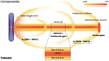 |
Fig. 16 Not-to-scale schematic cartoon displaying our findings on the HH211 protostellar jet and outflow. Different outflow components, line tracers, and temperature gradients (not-to-scale) are labelled. |
4 Discussion
MIRI-MRS observations have revealed the fine structure of a low-mass protostellar flow, its chemistry, physics and dynamics. As HH 211 is one of the best studied protostellar outflows, from optical to millimetric wavelengths, we can use ours and previous observations to draw the most up-to-date and complete picture of a low-mass protostellar flow.
4.1 A textbook case of a protostellar outflow
HH 211 can be considered a textbook case of a Class 0 pro-tostellar flow. Indeed, our observations reveal all the typical jet/outflow structures: a poorly collimated molecular wind, traced by cold H2 at 200–400 K; a stratified (layered) jet, traced by atomic and molecular gas; and large terminal BSs, which sweep up the circumstellar and interstellar medium, forming a large (less-collimated) molecular outflow traced by the warm/cold H2 (500–1500 K). A not-to-scale schematic sketch of our results is shown in Fig. 16, which depicts the main outflow components, line tracers and temperature gradients observed.
The jet onion-like radial structure is probably one of the most striking features observed in HH 211. We observe jet stratification in size, velocity, temperature, and chemistry, as predicted for jets originating from MHD disc-winds (see e.g. Panoglou et al. 2012; Pascucci et al. 2023). In extended MHD disc-wind models, the wind has an ‘onion-like’ kinematic and thermo-chemical structure, with streamlines launched from larger disc radii having lower velocity, temperature, and ionization, as well as a higher H2 abundance (see e.g. Panoglou et al. 2012; Wang et al. 2019; Pascucci et al. 2023). According to MHD disc-wind theory, such thermo-chemical gradients arise from a radially extended (~0.1–20au) disc-wind. As Keplerian velocities, chemical composition, density, and physical properties change across the disc radius, this would naturally produce an onion-like structured jet with different layers. Therefore, the different features observed are related to each other.
The jet’s innermost atomic component of HH 211 is produced by the fast flow (vtot ~130 km s−1), likely ejected from the inner gaseous disc. The inner atomic jet has electron temperatures of ~800–2000 K, very low electron densities ~ 100–400 cm−3, high pre-shock densities up to a few 105 cm−3, and very low ionisa-tion fraction (≲10−3). The most ionised region, traced by [Fe II] emission at higher excitation, is the core of the atomic jet, possibly surrounded by [S I] and [Fe I] at lower excitation energies. Unfortunately, MIRI does not have enough spectral and/or spatial resolution to differentiate these two possible components, which, in our data, have similar size and velocity.
The molecular jet layer is made of H2 that also shows a stratification in size, temperature and column density: the warm/hot component at higher temperature (1000–1500 K) and lower column density (1018–1019 cm−2) has a varying radius of 60–130 au and thus positioned in between the atomic and the cold/warm component at lower temperature (400–1000 K) and higher column density (1019–1020 cm−2) and radii of 100–180 au.
One could argue that SiO, and the fast CO jet components, detected at sub-millimetric and millimetric wavelengths (see e.g. Gueth & Guilloteau 1999; Lee et al. 2007, 2018), possibly arise from the H2 warm/hot region, on the basis of their observed velocities (~100 km s−1; see Jhan & Lee 2016, 2021), and temperatures (TCO =250–950 K and TSiO >250 K see Giannini et al. 2001; Nisini et al. 2002, , respectively) similarly to the warm/hot H2 component (see Table C.7 and Fig. 9).
Another important feature predicted by disc-wind models is dust removal from the disc and the presence of dust along the flows (see Panoglou et al. 2012). As disc winds extend well beyond the dust sublimation radius, they can lift dusty particles up to ~1 µm in size (Booth & Clarke 2021), which can be seen along the flow. Indeed, this is likely what we are observing in HH 211. We note that dust has also been recently detected in the environment of other Class 0 protostars with ALMA (see Cacciapuoti et al. 2024), but here it is also detected in a proto-stellar jet. Future MIRI/MRS observations from this and other programmes will tell whether this is a common feature in pro-tostellar jets, previously unseen with Spitzer, or rather it can be ascribed to the youth of this particular flow.
Our observations indicate significant differences in the dynamical properties of the jet components as seen from their onion-like structure. We note that the mass-ejection rates measured from the warm H2 component of the jet (Ṁjet(H2)=1− 1.6 × 10⁻⁶ M⊙ yr−1), match very well those from SiO and fast CO (1.1−1.8 × 10⁻⁶ M⊙ yr−1; see Sect. 3.7), showing that the warm molecular component is the primary mover of the outflow. In contrast, the mass-flux rate, momentum and momentum flux derived from the atomic component are up to one order of magnitude smaller than those inferred from the warm H2 component (see Tables 2 and 3). This confirms that the molecular jet is the dynamically most important component of the outflow contrary to the more evolved Class II jets, where the atomic component of the jet is the most important and drives the outflow (see, e. g. Ray et al. 2007). A similar result for young outflows was reported by Nisini et al. (2015); Sperling et al. (2021) who investigated [OI] 63 µm emission using SOFIA.
4.2 An onion-like flow launched by a disc-wind?
An interesting feature seen along the jet and depicted in Fig. 8 is the increase in the jet radius with distance to the source, evident for the atomic component, as expected in MHD wind models (e.g. Pascucci et al. 2023, and references therein). Despite the large uncertainties in the radius estimate of the different components (see Fig. 8), the atomic jet seems to show a larger opening angle with respect to the H2 components, which appear to be almost flat and surely collimated beyond 1000–1500 au in Fig. 8. In MHD wind models it should be the other way round, namely the opening angle of the atomic component should be narrower than that of the molecular one. These results might indicate that the H2 emission is tracing extended structures (likely small BSs rather than the jet) that are not fully spatially resolved (see e.g. the shape of Knot 4 and Knot 3 in Fig. 1 and upper panel of Fig. 4), or that the molecular jet recollimates at smaller distances from the source.
In any case, fitting the jet radius as a function of the distance to the source just provides a very crude approximation of the jet launching region (in X-winds; or the launching inner radius -rin - in extended disc-winds). To get a better estimate of rin, we can use the observed jet velocity, assuming that it is equal to the asymptotic speed of the jet poloidal velocity (see e.g. Ferreira et al. 2006; Panoglou et al. 2012). In this case, we can express the launching foot point (r0) as a function of the magnetic lever arm (λ), stellar mass (M*) and jet velocity (vtot):
 (3)
(3)
If the jet is ejected from a very small region (e.g. in X-winds and very compact disc-winds) λ ≃ Ṁacc/Ṁjet (see e. g. Pelletier & Pudritz 1992; Pascucci et al. 2023). From Sect. 3.7, we estimated Ṁjet/Ṁout ~0.12–0.19, and therefore we infer λ ~5–8, and we get r0 ~0.03–0.05 au from Eq. (3). This region is well within the dust sublimation radius (≳0.1 au) of a low-mass Class 0 pro-tostar (e. g., Lee 2020). This is in contrast with the detection of both dust and H2 emission along the jet of HH 211. It is then more likely that we are dealing with an extended disc-wind and thus r0 ~ rin (i. e. r0 matches the innermost radius of the jet launching region).
It is not possible to properly derive rout (i.e. the most external launching radius) from the data at our disposal, unless a discwind model is used (see Tabone et al. 2020; Lee et al. 2021). As the radius of the toroid/disc in HH 211 is ~20 au (Lee et al. 2019), we can assume this as an upper limit for rout.
In the past few years, ALMA observations at high-angular resolution have shown small-scale poorly collimated rotating molecular winds, launched from the discs of YSOs (e g., HH 212, DG Tau B, L1448-mm; see Lee et al. 2021; de Valon et al. 2020; Nazari et al. 2024). When both jet and molecular disc-wind ejection rates can be estimated, Ṁwind is about one order of magnitude higher than Ṁjet, suggesting that it is the slow-velocity disc-wind that removes much of the material from the disc rather than the jet itself (i.e. the re-collimated part of the disc-wind; see Pascucci et al. 2023, and discussion therein).
As we detect slow-moving, low density, poorly collimated warm H2 emission down to ~2″ (~650 au) from the source, we can assume that this H2 is tracing a poorly collimated disc-wind, rather than being circumstellar material swept-up by the jet. From the 0-0 S(1) velocity map, we infer radial velocities in the range of 4–5(±5) km s−1. We cannot adopt an inclination angle of 11° as the wind is not collimated. However, we can assume a typical wind angle of ~30° with respect of the disc plane, and therefore ~ 40° of inclination, and the wind velocity will be 6– 8(±8) km s−1. The emitting radius is about 4 times larger than the jet radius, and the column density is 3–6 × 1019 cm−2, namely 2-4 times lower than that of the jet. Therefore, the inferred discwind mass ejection rate (ṀDW) is of the same order of  , but cannot be much larger as measured in other sources (see Pascucci et al. 2023, and references therein). However, it is worth noting that we are measuring the wind at 650–1000 au from the driving source, as the visual extinction is too high to detect any emission closer to it. Therefore our ṀDW estimate is likely a lower limit of its real value.
4.3 Excitation conditions along the flow
Besides the onion-like structure discussed in Sects. 4.1 and 4.2, we also detect different physical conditions along the flow, moving from the inner jet to the outer BSs, in both molecular and atomic emission.
One of the most striking features in the H2 maps of Fig. 9 is the increase (by a factor of 2–3) in temperature, moving from the inner jet to the outer BSs as well as the symmetric decrease (by a factor of 2–3) in column density in both components. The atomic component shows a similar trend in Te, increasing by a factor of 2–3 from the jet to the BSs. On the other hand, the pre-shock density slightly decreases and ne slightly increases, and, overall, xe increases from ~10−3 to ~10−2 moving along the flow (see Tables 1 and 2). As the fast jet shocks the ambient medium at the four external BSs, the flow velocity drops, and radial velocity gradients are detected in both molecular and atomic lines (see Figs. 14, D.1, and D.2 and Tables C.6 and C.7).
This change in the physical excitation conditions along the flow is also seen in its chemistry, namely in the diversity of the spectra observed in the terminal BSs in contrast to the spectra seen along the jet.
For comparison, the jet emission is mostly characterised by atomic forbidden lines with low excitation energies (Eup ≲ 2700 K) and low ionisation potentials (I.P ≤ 7.9 eV; see Table C.2). In particular, it is the first time that [Fe I] is detected along a protostellar jet, and its coexistence with [Fe II] is very indicative of the low-ionisation of the flow. Besides relatively faint HD emission, the only molecular emission along the jet is H2 (the main cooler along the whole flow) with transitions at relatively low excitation energies (Eup ≲ 7200 K; see Table C.1).
In contrast to the jet, the emission at the terminal BSs (BS 1–BS 3) shows atomic forbidden lines at much higher excitation energies (Eup ≲ 14 600 K), and ionisation potentials (I.P ≤ 23.81 eV). Notably, [Fe I] emission mostly or completely disappear and [S III] is just about detected, indicating that the atomic species are much more ionised here. It is also worth noting that [S I] at 25 µm is still extremely bright, having similar I.P. and Eup of [Fe I] line at 24 µm. This is due to the fact that, as predicted in J-shock models (e. g. Hollenbach & McKee 1989), the [S I] line intensity is 1–2 orders of magnitude higher than that of [Fe I] for pre-shock densities of n0 ~104 cm−3 (see Fig. 7 in Hollenbach & McKee 1989). Nevertheless, [S II] optical emission has been observed at the BSs (see Walawender et al. 2005, 2006), which provides further evidence that the atomic component is partially ionised.
Moreover, the terminal BSs (BS1–BS 3) display an extremely rich molecular emission. Along with HD and H2 transitions at high excitation energies (Eup up to 16 000 K; however NIRSpec spectra reveal v = 5 transitions with Eup up to ~30000K; Ray et al. 2023), our MIRI spectra show bright CO (1-0) emission from the high-J P-branch at 2000–3000 K (see also NIRSpec spectra in Ray et al. 2023), OH, H2O, CO2, and HCO+. In particular, the detection of suprathermal OH rotational emission, as well as H I emission in BS 3, namely Hα (Walawender et al. 2005, 2006) and Paα in the NIRSpec spectra (but no Brα; Ray priv. comm.), indicates that a UV radiation field, produced by a relatively fast J-shock, must be present to photodissociate H2O by Lyα radiation. Notably, the inferred shock velocity at the brightest BS (BS 3, vs=45±5 km s−1; see Table 2) matches well the shock velocity predicted by Tabone et al. (2020) (50 km s−1) to reproduce the suprathermal OH rotational emissions in HH 211 terminal BSs. Intermediate velocity (25-60 km s−1), stationary, weakly magnetised, J-type, molecular shocks are also able to reproduce many other molecular (e.g., H2, HCO+, CO, CO2, H2O) as well as atomic features observed in HH 211 (e. g., H I, [S I], [S II], [O I], [Fe II]; see Lehmann et al. 2020, 2022). However, the Lehmann et al. (2020) fiducial shock-model (vs=40 km s−1, nH=104 cm−3) provides electron temperatures of about one order of magnitude higher than what we measured in BS 3 (104 vs. 103 K), suggesting that we are not exactly probing the same regions of the shock with the [Fe II].
The overall picture of the HH 211 blue-lobe indicates that a relatively fast-moving, mostly molecular and weakly shocked jet is impinging the ambient medium, generating moderate J-shocks at the terminal BSs. Unfortunately, only upper limits of the jet shock-velocity (vs <60 km s−1) are available from our analysis. Nevertheless, assuming that the shock velocity broadens the line profile, we can compare the FWHM of the [Fe II] 5.3 µm line along the jet and at the terminal BSs and check whether the line is narrower along the jet. At the shortest wavelengths of MIRI, the line width is spectroscop-ically marginally resolved at the BSs, whereas the H2 lines are not resolved. We measure FWHM([Fe II])=19±0.9 Å, and FWHM(H2)=17±0.1 Å, which provides a deconvolved FWHM of 8.5±0.9 Å (i.e. Δv=48±5 km s−1). On the other hand, the [Fe II] line is not spectrally resolved along the jet, namely at Knot 5 and Knot 2, where it is detected at relatively high S/N, as its FWHM matches that of the H2 0-0 S(7), indicating that the shock velocity along the jet is smaller than at BS 3.
4.4 Comparing HH 211 flow properties with other Class 0 and more evolved flows
Spatially resolved flows in Class 0, I, and II sources share many features in common, including collimated jets, wider winds, and outflows, implying that the accretion/ejection mechanisms are similar over a wide range of stellar masses and over the whole star formation process. However, a closer look shows that physical, chemical, and dynamical properties of the flow change as the central source evolves from the protostellar to the pre-main sequence phase. In particular, it is worth noting that the jet’s atomic component becomes dominant moving from the protostellar to the Class II stage, when the molecular component of the jet mostly or totally disappears, being fully dissociated, and the molecular emission is mostly or fully relegated to winds and entrained outflows. Jets become gradually faster (from 100 km s−1 in Class 0 to 300–400 km s−1 in Class II) and less dense (from 105–106 to 103–104 cm−3), the gas excitation conditions along the flow increase, showing a higher ionisation fraction (from 10−3–10−2 to 0.2-0.5) and electron temperature (from 102–103 to 104 K) (see, e. g. Ray et al. 2007; Nisini et al. 2015; Podio et al. 2021). At the same time, mass-flux rates decrease (from 10−5–10−6 to 10−8–10−10 M⊙ yr−1), as less matter is available in the disc to be ejected or accreted onto the forming star.
While the overall picture becomes more and more clear, as the studied sample of YSOs increases in number, still, flows driven by the same class of objects show significant differences in terms of chemistry, excitation conditions, and morphology. Although some differences might be related to the different mass of the accreting source (see e.g. Federman et al. 2024), different ages and binarity of the central protostar (Tychoniec et al. 2024), or differences in the accretion and ejection rates, similar objects at the same evolutionary stage still present variations. Indeed, as different JWST programmes are providing us with new and exciting MIR data of spatially and spectrally resolved protostellar jets (see e.g. Yang et al. 2022; Narang et al. 2024; Federman et al. 2024; Tychoniec et al. 2024; Nisini et al. 2024; Rubinstein et al. 2024), we have now the chance to study and compare sources with similar mass and age, using similar tracers in the MIR regime.
For example, we can now compare the flow properties of HH211 with those of IRAS 16253-2429 (Narang et al. 2024), a Class 0 low-luminosity protostar (Lbol=0.2 L⊙, M*=0.12– 0.17 M⊙), observed with both MIRI and NIRSpec. Despite the similar mass and evolutionary stage of these protostars, there are several striking differences between the two flows. The IRAS 16253-2429 jet is more atomic than molecular and more ionised than HH211, as no [Fe I] emission is detected, [S I] emission is confined to close to the source, and [Ne II] and Brα emission are well detected along the flow (see Fig. 1, 2, and 3 in Narang et al. 2024). The pre-shock density is two orders of magnitude lower (2× 103 cm−3; Narang et al. 2024), shock velocities are similar or slightly higher (~54 km s−1) than in HH 211, jet velocities of the [Fe II] component are similar or higher (vtot=169±15 km s−1), mass-flux rates are extremely low (~0.4–1.1 × 10⁻¹⁰ M⊙ yr−1; Narang et al. 2024) with respect to what measured in HH 211. This is very likely connected to IRAS 16253-2429 having a very low mass-accretion rate (Ṁacc=2.4±0.8 × 10⁻⁹ M⊙ yr−1; Watson et al., in prep.), and it is reflected in the one order of magnitude difference in bolometric luminosity between the two Class 0 sources.
On the other hand the size of the two atomic jets seem to be roughly comparable. The diameter of the IRAS 16253-2429 jet at 400 au from the source (i.e. at the largest distance measured there) is ~60au Narang et al. (2024), whereas the HH 211 jet width at Knot 1R (~580 au), the closest marginally resolved knot, has a size of 90±30 au. Unfortunately, further comparison is not possible, as the HH 211 innermost jet emission (in [Fe II]) is not spatially resolved.
Overall, the disparity in accretion/ejection activity, reflected in the YSO bolometric luminosity, might be key to explain such observational differences. However, comparing the flow morphology and chemistry of HH 211 with the outflows associated with B335 and HOPS 153 (Class 0 YSOs, slightly more massive than HH 211 but with similar Lbol; see Table 1 in Federman et al. 2024) presented in Federman et al. (2024), we still note significant differences in terms of their morphology and jet excitation. In particular, in B335 and HOPS 153, H I Brα emission from the jet is detected, H2 emission is more confined towards the winds and outflow cavities and is faint along the jet (see Figs. 3 and 4 in Federman et al. 2024). Hodapp et al. (2024) JWST/NIRCAM images of B335 reveal CO and H2 emission in several knots along the jet.
While some morphological differences among HH 211, B335 and HOPS 153 can be ascribed to the different wavelength regimes (NIRSpec 2.8-5 µm vs. MIRI 5-28 µm), tracing somewhat different excitation conditions of the gas, nevertheless the excitation conditions appear to be dissimilar.
In contrast, by comparing the HH 211 jet properties with those of Class 0 sources with similar Lbol, presented in Podio et al. (2021) (i. e. the CALYPSO IRAM-PdBI survey), we note that, in several cases (e.g. IRAS 4A and 4B sources), jet width and dynamical properties (i.e. Ṁjet and Ṗjet) of the HH 211 warm H2 component are similar to those derived for SiO and CO high-velocity components (see Table 3 and Fig. 5 in Podio et al. 2021), despite observing different wavelength regimes. Nevertheless, although Ṁjet is correlated to Lbol, the CALYPSO survey shows significant dispersion (at least one order of magnitude) in the mass ejection rates of Class 0 sources with similar Lbol.
The cause of such a scattering is not yet clear. Episodic accretion could be one of the possible explanations, and the presence of several knots along the flows surely hints to some variability. Nevertheless, as Lbol of Class 0 sources derives from their accretion luminosity (Lacc ~ GṀaccM*/R*), the latter should be strictly correlated with their mass accretion and ejection rates, and it is thus difficult to explain such large spreads. Of course one possible cause of such discrepancies could be that the Ṁjet/Ṁacc efficiency varies from source to source depending, for example, on magnetic properties. Alternatively our M*/R* estimates are wrong, or the selected samples of Class 0 YSOs include proto-stars with different ages and accretion rates. As our sample of Class 0 protostars observed with JWST becomes larger, we might have the chance to answer these questions.
5 Conclusions
We present JWST MIRI-MRS spectral maps (5-28 µm) of the HH 211 flow, covering the blueshifted lobe, the central proto-star, and a small portion of the redshifted lobe. The analysis of these maps provides an unprecedented view of the flow physics, chemistry, and excitation conditions of the flow, as well as of its kinematics and dynamical properties. The central protostar is not detected. Ancillary JWST NIRCam H2 narrow-band images at 2.12 and 3.25 µm (1-0 S(1) and 1-0 O(5) lines, respectively) provide a visual-extinction map of the whole flow and are used to deredden our images and spectra in the analysis. The visual extinction ranges from 5–15 mag at the terminal BSs up to 20– 60 mag along the bipolar jet towards the central source. As the inner jet regions (within ~5 of the source) are not detected at 2.12 µm, we use a value of 80 mag - as inferred from H2 ro-vibration diagrams – to correct for visual extinction in these regions. Our main conclusions can be summarised as follows:
The overall morphology of the flow consists of a highly collimated jet - which is both atomic ([Fe I], [Fe II], [S I], [Ni II]) and molecular (H2, HD) - that shocks the ambient medium, producing several large BSs, as well as driving a large molecular (H2) outflow, mostly traced by H2 0-0 transitions at low-J. Further H2 0-0 S(1) uncollimated emission is also detected down to 2″ – 3″ from the source, tracing a less collimated wind.
The inner jet, within ~2.5″ of the source, is mostly traced by atomic emission, and the lack of H2 emission is likely due to the large visual extinction (AV >80 mag) close to the source. The [Fe II] emission at 26 µm is detected down to ~ 130 and 300 au from the source on the jet red- and blueshifted side, respectively.
In contrast to the relatively small number of atomic and molecular species detected in the jet, the terminal BSs (especially BS 3) are very rich in chemistry with many forbidden atomic ([Cl I], [Cl II], [AR II], [Co II], [Ne II], [S III]) and molecular (CO, OH, H2O, CO2, HCO+) species detected. In particular, suprathermal OH rotational emission (between 9.1 and 25 µm) originating from water photodis-sociation (114–143 nm UV radiation produced by strong -vs ≥40 km s−1 - shocks) is observed.
Dust-continuum emission (at T ~90 K) is detected at the terminal BSs (BS 1–3) that roughly matches the [Fe II] spatial emission at 26 µm, and more faint emission is detected in the blue- and redshifted jet. Although some or most of the dust in the external BSs likely originates from the circumstellar or interstellar environment, the continuum emission detected in the inner jet must arise from dust lifted from the disc. This is also supported by the dust-to-gas mass ratio (≤10+3) inferred along the jet.
Line maps show that the HH 211 jet is marginally resolved in diameter. Our analysis reveal a jet with an onion-like structure, with the atomic jet displaying a smaller size and the molecular component extending to larger radii. The different atomic lines show similar values in radius (ranging from ~45 to ~100 au), and the H2 lines have radii similar to or larger than the atomic jet. The radius of the 0-0 S(7) line ranges from ~60 to ~130 au, whereas the 0-0 S(1) line is positioned on the outer layers of the jet (~ 100–180 au).
We built maps of the H2 excitation conditions
 along the flow. The H2 emission shows a stratification in temperature, and we fitted two components, referred to as the warm (W) and hot (H) component.
  (W) along the jet varies from ~300K close to the source to 500–700 K reaching 900–1000K in the outer BSs. Its column density changes from 1019 to 1020 cm−2 along the jet, while it is only 1019 cm−2 along the BSs, except in BS 3 (~3 × 1020 cm−2).
  varies from 1000 to 2000 K along the jet, whereas it is much higher (2000-3500 K) at the terminal BSs. Its column density is higher along the jet (1−2 × 1019 cm−2) and drops in the outer jet and BSs (1018−1019 cm−2).
The less collimated wind close to the source is colder (200– 400 K) and less dense (1018–1019 cm−2) than the jet. The outflow gas (i.e. the entrained gas) is less dense and colder than the jet and BSs.
Te and ne are derived from [Fe II] line fluxes using an NLTE code. Moving away from the source, Te increases from ~1000 to ~1400K at BS 4. The terminal BSs show the highest electron temperatures (1800-3800 K). A similar trend is seen for ne, with low electron densities (150–400 cm−3) along the jet and at BS 4, and higher values (350–800 cm−3) at the three terminal BSs.
We inferred the [Fe II] gas-phase abundance along the jet using Hollenbach & McKee (1989) J-shock models. Iron is largely depleted along the flow and just a small amount is in gas-phase (between ~2 and ~10%), with abundances ranging from ~7 × 10⁻⁷ to ~3 × 10⁻⁶. Surprisingly, jet knots close to the source seem to be less depleted than those positioned further away from the source. We argue that this might be the result of different shock conditions along the jet.
The Hollenbach & McKee (1989) J-shock models also allow us to infer the pre-shock density, shock velocity, and ionisa-tion fraction along the flow. n0 varies from ~1−2 × 105 cm−3 in the inner jet to ~0.4−0.9 × 105 cm−3. Shock velocities at the terminal BSs range from 35±5 to 45±5 km s−1, whereas only upper limits (vs <45-60 km s−1) can be derived for the jet. The ionisation fraction varies from 10−3 along the jet to 10−2 at the terminal BSs.
We also constructed radial velocity maps for both molecular (H2) and atomic lines ([S I], [Fe I], [Fe II]). Overall, the atomic lines show similar velocities. Average values of vr= −25±5 and 25±5 km s−1 are found in the blue- and red-shifted inner jet, which correspond to a total velocity of v= 130±25 km s−1, for a jet inclination of 11º. The radial velocity of the atomic component peaks at −30±5 km s−1 (vtot=160±25 km s−1) in the outer jet and drops at the terminal BSs. The kinematics of the H2 shows a behaviour similar to the atomic lines, but has radial velocities of ~ 10 km s−1 lower than the atomic component. An average jet inclination angle (with respect to the plane of the sky) of 11°.6+0°.6 is inferred from H2 radial and tangential velocities (Ray et al. 2023). On the other hand, the terminal BSs show a much larger spread in i, ranging from 5°.5+4°.4 to 19°4+2°.1.
Mass flux rate, momentum, and momentum flux of the different knots of the jet are inferred for the H2 (warm and hot) and atomic components. Ṁ, P, and P values of the warm H2 component are up to one order of magnitude higher than those inferred from the atomic component, whereas the hot H2 component shows jet dynamical values similar to those of the atomic component. Our findings indicate that the warm H2 component is the main driver of the outflow, namely it is the most significant dynamical component of the jet, which is in contrast to jets from more evolved YSOs.
Overall, our JWST MIRI/MRS maps of HH211 reveal a textbook case of a protostellar flow, revealing a collimated jet with an onion-like structure comprised of layers of different size, velocity, temperature, and chemical composition. The jet is dusty, possibly launched by a disc-wind, and is mostly molecular, and its warm H2 component is the main driver of the molecular outflow. The jet close to the source is surrounded by a U- or V-shaped, less-dense, and colder molecular wind. Excitation conditions also vary along the flow. Further JWST observations of other young Class 0 and Class I jets and outflows will show whether the characteristics presented here for HH211 are common to young jets or that the flow properties markedly evolve with time, as early indications suggest.
Acknowledgements
We would like to thank the referee for their helpful suggestions as well as Marta Tychoniec for drawing the HH211 cartoon shown in Fig. 16. A.C.G. would like to thank David Hollenbach for helpful discussions and for sharing the HM89 code, as well as Juan Alcalá for his useful comments. This work is based on observations made with the NASA/ESA/CSA James Webb Space Telescope. The data were obtained from the Mikulski Archive for Space Telescopes at the Space Telescope Science Institute, which is operated by the Association of Universities for Research in Astronomy, Inc., under NASA contract NAS 5-03127 for JWST. These observations are associated with program ID 1257. The NIRCam observations presented here were made from the Guaranteed Time Allocation to MJM upon selection as an Interdisciplinary Scientists on the JWST Science Working Group in response to NASA AO-01-OSS-05 issued in 2001. The following National and International Funding Agencies funded and supported the MIRI development: NASA; ESA; Belgian Science Policy Office (BELSPO); Centre Nationale d’Etudes Spatiales (CNES); Danish National Space Centre; Deutsches Zentrum fur Luft- und Raumfahrt (DLR); Enterprise Ireland; Ministerio De Economiá y Competividad; Netherlands Research School for Astronomy (NOVA); Netherlands Organisation for Scientific Research (NWO); Science and Technology Facilities Council; Swiss Space Office; Swedish National Space Agency; and UK Space Agency. A.C.G. acknowledges support from PRIN-MUR 2022 20228JPA3A “The path to star and planet formation in the JWST era (PATH)” funded by NextGeneration EU and by INAF-GoG 2022 “NIR-dark Accretion Outbursts in Massive Young stellar objects (NAOMY)” and Large Grant INAF 2022 “YSOs Outflows, Disks and Accretion: towards a global framework for the evolution of planet forming systems (YODA)”. T.P.R. acknowledges support from ERC grant 743029 EASY. H.B. acknowledges support from the Deutsche Forschungsgemeinschaft in the Collaborative Research Center (SFB 881) “The Milky Way System” (subproject B1). E.v.D., M.v.G., L.F., K.S., W.R. and H.L. acknowledge support from ERC Advanced grant 101019751 MOLDISK, TOP-1 grant 614.001.751 from the Dutch Research Council (NWO), the Netherlands Research School for Astronomy (NOVA), the Danish National Research Foundation through the Center of Excellence “InterCat” (DNRF150), and DFGgrant 325594231, FOR 2634/2. P.J.K. acknowledges financial support from the Science Foundation Ireland/Irish Research Council Pathway programme under Grant Number 21/PATH-S/9360. K.J. acknowledges the support from the Swedish National Space Agency (SNSA). G.P. gratefully acknowledges support from the Max Planck Society. This research has made use of NASA’s Astrophysics Data System Bibliographic Services. This research made use of NumPy (Harris et al. 2020); Astropy, a community-developed core Python package for Astronomy (Astropy Collaboration 2013, 2018); Matplotlib (Hunter 2007); pdrtpy (Kaufman et al. 2006; Pound & Wolfire 2008, 2011, 2023).
Appendix A Additional MIRI-MRS maps
Figure A.1 shows a tricolour MIRI-MRS map of H2 of H2 0-0 S(7) (at 5.5 µm,in blue), [S I] (at 25.2 µm,in green), and [Fe II] (at 26 µm, in red) emission lines. H2 emission (0-0 S(1) line at 17.0 µm) is overplotted with magenta contours (at 3, 10, 20, 50, 100, 200, and 500 σ; 1 σ=40 MJy sr−1).
Figure A.2 presents the MIRI-MRS intensityintegratedmaps of the following transitions (from top to bottom): HD0-0 R(4) at 23.03 µm, CO (1-0) lines (from P29 to P31) from 4.96 to 4.98 µm, [Ni II] at 6.64 µm, [Cl I] at 11.33 µm.
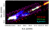 |
Fig. A.1 Tricolour MIRI-MRS map of H2 0-0 S(7) (at 5.5 µm, in blue), [SI] (at 25.2µm, in green), and [FeII] (at 26µm, in red) emission lines. H2 0-0 S(7) (at 17.0 µm) magenta contours (at 3, 10, 20, 50, 100, 200, and 500 σ; 1 σ=40 MJy sr−1) are also overplotted. The white circle marks the position of the ALMA mm continuum source. |
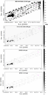 |
Fig. A.2 Additional line maps of some bright features detected along HH211. From top to bottom: HD0-0R(4) at 23.03 µm, CO (10) lines from 4.96 to 4.98 µm, [Ni II] at 6.64 µm, [Cl I] at 11.33 µm. The magenta circle shows the position of the ALMA mm continuum source. Integrated flux is in mJy pixel−1. |
Appendix B AV estimate in the inner-jet region and Boltzmann plots
Figure B.1 shows the H2 ro-vibrational diagram for the blueshifted inner jet extracted at R.A.(J2000): 03h43m57.s 176, Dec.(J2000): +32°00′48.″18, namely about 4.″5 (towards the SE) away from the position of the mm ALMA source. Only pure rotation lines are detected and reported, as the v = 1 lines are too faint to be detected. Two temperature components (warm and hot) are visible and fitted. Values of T(H2) and N(H2) for both components are reported. Fits were obtained by varying AV values, until the best fit (highest correlation coefficient) was derived. Inferred uncertainty in AV is about 10 mag.
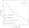 |
Fig. B.1 Ro-vibrational diagram towards the inner jet of HH211 (R.A.(J2000): 03h43m57.s l76, Dec.(J2OOO): +32°00′48.″18) at ~4.″5 away from the source. Two temperature components are fitted. AV = 80 mag best fits the two gas components. |
Figure B.2 show two examples of Boltzmann plots derived by our routine to compute the excitation maps. Spectra were extracted from a single spaxel in the blueshifted inner jet (top panel) and in the wings of BS 3 (bottom panel).
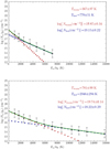 |
Fig. B.2 Examples of pixel-by-pixel ro-vibrational diagram towards HH211. Top panel: ro-vibrational diagram in the blueshifted inner jet (R.A.(J2000): 03h43m57.469, Dec.(J2000): +32°00′47.″33), where only v = 0 lines (up to S(7)) are detected. In this case, temperature of both components is low and column density is high. Bottom panel: ro-vibrational diagram towards the wing of BS 3 (R.A.(J2000): 03h43m59.s 277, Dec.(J2000): +32°00′35.″13), where both v = 0 and v = 1 lines are detected. In this case, the temperature of both components is high and the column density is low. |
Appendix C Additional tables
Table C.1 provides the list of identified H2 transitions along with their theoretical wavelength (in µm), energy of the upper level (in K), and corresponding MIRI Channel/Grating.
Table C.2 provides a list of the forbidden atomic lines identified along the HH2ll flow. The table also reports the ionisation potential of the species, transition Ш, wavelength, excitation temperature of the upper level, the corresponding MIRI Channel/Grating and the outflow regions where the line was detected.
Table C.3 lists the HD transitions detected as well as their wavelength, energy of the upper level, and corresponding MIRI Channel/Grating.
Table C.4 reports, for each identified knot and each species, its FWHM in arcseconds (measured orthogonally to the jet axis), the corresponding size (deconvolved for the FWHM of the corresponding PSF), and its radius in au.
As an example of the extracted spectra, Table C.5 lists identified lines, wavelengths, line fluxes and uncertainties in Knot 2. Spectrum and identified lines are also shown in Fig. 5.
For each knot and BS identified, Table C.6 reports measured radial velocities and their uncertainties, along with the total velocities derived by assuming an average inclination angle of 11° with respect to the plane of the sky.
Detected H2 pure rotational lines in the jet and BSs.
Detected atomic lines in the jet and bow shocks.
For each knot and BS identified, Table C.7 reports the radial velocity of the H2 0-0 S(1) and 0-0 S(7) lines, the tangential velocity of the H2 1-0 S(1) line as measured by Ray et al. (2023), the total velocity of the hot and warm component, and the inclination angle of the feature with respect to the plane of the sky.
Detected HD transitions.
Size of knots in the inner jet
Detected lines and fluxes in Knot 2.
[Fe II] radial velocity values along the HH 211 flow
H2 velocities, inclination along the HH 211 flow
Appendix D Additional MIRI-MRS velocity maps
In this section additional velocity maps of the brightest detected atomic species ([S I] at 25 µm and [Fe I] at 24 µm; top and bottom panel of Fig. D.1, respectively) and H2 transitions (0-0 S(1) and 0-0 S(7); top and bottom panel of Fig. D.2, respectively) are presented.
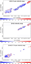 |
Fig. D.1 [S I] at 25 µm (top panel) and [Fe I] at 24 µm (middle panel) and [Fe II] at 17.9 µm (bottom panel) velocity maps. Black contours in the top and bottom panels show the integrated continuum-subtracted line intensity at 5σ (0.8 mJy pixel−1). Bottom panel black contours are at 5, 50, 100, and 500 σ (namely, 0.5, 5, 10, and 50 mJy pixel−1 Only velocities within a 5σ threshold are plotted. The magenta circle shows the position of the ALMA mm continuum source. |
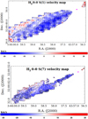 |
Fig. D.2 Top panel: H2 velocity map of the 0-0 S(1) at 17µm. Black contours show the integrated continuum-subtracted line intensity at 5, 10, 50, 100, and 200 σ (namely, 0.5, 1, 5, 10, and 20 mJy pixel−1). Bottom panel: H2 velocity map of the 0-0 S(7) at 5 µm. Black contours show the integrated continuum-subtracted line intensity at 5, 50, 100, 200, and 500 σ (namely, 0.1, 1, 2, 4, and 10 mJy pixel−1). Only velocities within a 5σ threshold are plotted in both panels. The magenta circle shows the position of the ALMA mm continuum source. |
References
- Argyriou, I., Glasse, A., Law, D. R., et al. 2023, A&A, 675, A111 [NASA ADS] [CrossRef] [EDP Sciences] [Google Scholar]
- Asplund, M., Amarsi, A. M., & Grevesse, N. 2021, A&A, 653, A141 [NASA ADS] [CrossRef] [EDP Sciences] [Google Scholar]
- Astropy Collaboration (Robitaille, T. P., et al.) 2013, A&A, 558, A33 [NASA ADS] [CrossRef] [EDP Sciences] [Google Scholar]
- Astropy Collaboration (Price-Whelan, A. M., et al.) 2018, AJ, 156, 123 [Google Scholar]
- Bachiller, R., Cernicharo, J., Martin-Pintado, J., Tafalla, M., & Lazareff, B. 1990, A&A, 231, 174 [NASA ADS] [Google Scholar]
- Bally, J. 2016, ARA&A, 54, 491 [Google Scholar]
- Bautista, M. A., & Kallman, T. R. 2001, ApJS, 134, 139 [Google Scholar]
- Beuther, H., van Dishoeck, E. F., Tychoniec, L., et al. 2023, A&A, 673, A121 [NASA ADS] [CrossRef] [EDP Sciences] [Google Scholar]
- Booth, R. A., & Clarke, C. J. 2021, MNRAS, 502, 1569 [NASA ADS] [CrossRef] [Google Scholar]
- Bushouse, H., Eisenhamer, J., Dencheva, N., et al. 2023, JWST Calibration Pipeline, https://zenodo.org/records/7714020 [Google Scholar]
- Cacciapuoti, L., Testi, L., Podio, L., et al. 2024, ApJ, 961, 90 [NASA ADS] [CrossRef] [Google Scholar]
- Caratti o Garatti, A., Giannini, T., Nisini, B., & Lorenzetti, D. 2006, A&A, 449, 1077 [NASA ADS] [CrossRef] [EDP Sciences] [Google Scholar]
- Caratti o Garatti, A., Stecklum, B., Linz, H., Garcia Lopez, R., & Sanna, A. 2015, A&A, 573, A82 [NASA ADS] [CrossRef] [EDP Sciences] [Google Scholar]
- Carr, J. S., & Najita, J. R. 2014, ApJ, 788, 66 [NASA ADS] [CrossRef] [Google Scholar]
- Cerqueira, A. H., Velázquez, P. F., Raga, A. C., Vasconcelos, M. J., & de Colle, F. 2006, AIP Conf. Ser., 875, 285 [NASA ADS] [CrossRef] [Google Scholar]
- Colangeli, L., Henning, T., Brucato, J. R., et al. 2003, A&A Rev., 11, 97 [NASA ADS] [CrossRef] [Google Scholar]
- De Colle, F., Cerqueira, A. H., & Riera, A. 2016, ApJ, 832, 152 [NASA ADS] [CrossRef] [Google Scholar]
- de Valon, A., Dougados, C., Cabrit, S., et al. 2020, A&A, 634, L12 [NASA ADS] [CrossRef] [EDP Sciences] [Google Scholar]
- de Valon, A., Dougados, C., Cabrit, S., et al. 2022, A&A, 668, A78 [NASA ADS] [CrossRef] [EDP Sciences] [Google Scholar]
- Decleir, M., Gordon, K. D., Andrews, J. E., et al. 2022, ApJ, 930, 15 [NASA ADS] [CrossRef] [Google Scholar]
- Dionatos, O., Nisini, B., Garcia Lopez, R., et al. 2009, ApJ, 692, 1 [NASA ADS] [CrossRef] [Google Scholar]
- Dionatos, O., Nisini, B., Cabrit, S., Kristensen, L., & Pineau Des Forêts, G. 2010, A&A, 521, A7 [NASA ADS] [CrossRef] [EDP Sciences] [Google Scholar]
- Dionatos, O., Ray, T., & Güdel, M. 2018, A&A, 616, A84 [NASA ADS] [CrossRef] [EDP Sciences] [Google Scholar]
- Dougados, C., Cabrit, S., Ferreira, J., et al. 2004, Ap&SS, 293, 45 [NASA ADS] [CrossRef] [Google Scholar]
- Dunne, L., Eales, S., Edmunds, M., et al. 2000, MNRAS, 315, 115 [Google Scholar]
- Federman, S. A., Megeath, S. T., Rubinstein, A. E., et al. 2024, ApJ, 966, 41 [CrossRef] [Google Scholar]
- Ferreira, J., Dougados, C., & Cabrit, S. 2006, A&A, 453, 785 [NASA ADS] [CrossRef] [EDP Sciences] [Google Scholar]
- Frank, A., Ray, T. P., Cabrit, S., et al. 2014, in Protostars and Planets VI, eds. H. Beuther, R. S. Klessen, C. P. Dullemond, & T. Henning (Tucson: University of Arizona Press), 451 [Google Scholar]
- Franz, R., Picogna, G., Ercolano, B., & Birnstiel, T. 2020, A&A, 635, A53 [EDP Sciences] [Google Scholar]
- Froebrich, D. 2005, ApJS, 156, 169 [Google Scholar]
- Fuente, A., Rivière-Marichalar, P., Beitia-Antero, L., et al. 2023, A&A, 670, A114 [NASA ADS] [CrossRef] [EDP Sciences] [Google Scholar]
- Giacalone, S., Teitler, S., Königl, A., Krijt, S., & Ciesla, F. J. 2019, ApJ, 882, 33 [NASA ADS] [CrossRef] [Google Scholar]
- Giannini, T., Nisini, B., & Lorenzetti, D. 2001, ApJ, 555, 40 [Google Scholar]
- Giannini, T., McCoey, C., Caratti o Garatti, A., et al. 2004, A&A, 419, 999 [NASA ADS] [CrossRef] [EDP Sciences] [Google Scholar]
- Giannini, T., Nisini, B., Antoniucci, S., et al. 2013, ApJ, 778, 71 [NASA ADS] [CrossRef] [Google Scholar]
- Gieser, C., Beuther, H., van Dishoeck, E. F., et al. 2023, A&A, 679, A108 [NASA ADS] [CrossRef] [EDP Sciences] [Google Scholar]
- Gueth, F., & Guilloteau, S. 1999, A&A, 343, 571 [NASA ADS] [Google Scholar]
- Harris, C. R., Millman, K. J., van der Walt, S. J., et al. 2020, Nature, 585, 357 [NASA ADS] [CrossRef] [Google Scholar]
- Hodapp, K. W., Chu, L. L., Greene, T., et al. 2024, AJ, 167, 102 [NASA ADS] [CrossRef] [Google Scholar]
- Hollenbach, D., & McKee, C. F. 1989, ApJ, 342, 306 [Google Scholar]
- Hunter, J. D. 2007, Comp. Sci. Eng., 9, 90 [NASA ADS] [CrossRef] [Google Scholar]
- Jhan, K.-S., & Lee, C.-F. 2016, ApJ, 816, 32 [NASA ADS] [CrossRef] [Google Scholar]
- Jhan, K.-S., & Lee, C.-F. 2021, ApJ, 909, 11 [NASA ADS] [CrossRef] [Google Scholar]
- Jones, A. P. 2000, J. Geophys. Res., 105, 10257 [NASA ADS] [CrossRef] [Google Scholar]
- Jones, O. C., Álvarez-Márquez, J., Sloan, G. C., et al. 2023, MNRAS, 523, 2519 [Google Scholar]
- Kaufman, M. J., Wolfire, M. G., & Hollenbach, D. J. 2006, ApJ, 644, 283 [Google Scholar]
- Kristensen, L. E., van Dishoeck, E. F., Bergin, E. A., et al. 2012, A&A, 542, A8 [NASA ADS] [CrossRef] [EDP Sciences] [Google Scholar]
- Law, D. D., Morrison, J. E., Argyriou, I., et al. 2023, AJ, 166, 45 [NASA ADS] [CrossRef] [Google Scholar]
- Lee, C.-F. 2020, A&A Rev., 28, 1 [NASA ADS] [CrossRef] [Google Scholar]
- Lee, C.-F., Ho, P. T. P., Hirano, N., et al. 2007, ApJ, 659, 499 [NASA ADS] [CrossRef] [Google Scholar]
- Lee, C.-F., Hasegawa, T. I., Hirano, N., et al. 2010, ApJ, 713, 731 [NASA ADS] [CrossRef] [Google Scholar]
- Lee, C.-F., Hwang, H.-C., Ching, T.-C., et al. 2018, Nat. Commun., 9, 4636 [NASA ADS] [CrossRef] [Google Scholar]
- Lee, C.-F., Kwon, W., Jhan, K.-S., et al. 2019, ApJ, 879, 101 [NASA ADS] [CrossRef] [Google Scholar]
- Lee, C.-F., Tabone, B., Cabrit, S., et al. 2021, ApJ, 907, L41 [NASA ADS] [CrossRef] [Google Scholar]
- Lehmann, A., Godard, B., Pineau des Forêts, G., & Falgarone, E. 2020, A&A, 643, A101 [EDP Sciences] [Google Scholar]
- Lehmann, A., Godard, B., Pineau des Forêts, G., Vidal-García, A., & Falgarone, E. 2022, A&A, 658, A165 [CrossRef] [EDP Sciences] [Google Scholar]
- Machida, M. N. 2014, ApJ, 796, L17 [CrossRef] [Google Scholar]
- McCaughrean, M. J., Rayner, J. T., & Zinnecker, H. 1994, ApJ, 436, L189 [NASA ADS] [CrossRef] [Google Scholar]
- McClure, M. 2009, ApJ, 693, L81 [NASA ADS] [CrossRef] [Google Scholar]
- Millard, J. S., Eales, S. A., Smith, M. W. L., et al. 2020, MNRAS, 494, 293 [NASA ADS] [CrossRef] [Google Scholar]
- Moraghan, A., Lee, C.-F., Huang, P.-S., & Vaidya, B. 2016, MNRAS, 460, 1829 [NASA ADS] [CrossRef] [Google Scholar]
- Mottram, J. C., van Dishoeck, E. F., Kristensen, L. E., et al. 2017, A&A, 600, A99 [NASA ADS] [CrossRef] [EDP Sciences] [Google Scholar]
- Narang, M., Manoj, P., Tyagi, H., et al. 2024, ApJ, 962, L16 [NASA ADS] [CrossRef] [Google Scholar]
- Nazari, P., Tabone, B., Ahmadi, A., et al. 2024, A&A, 686, A201 [NASA ADS] [CrossRef] [EDP Sciences] [Google Scholar]
- Neufeld, D. A., Nisini, B., Giannini, T., et al. 2009, ApJ, 706, 170 [NASA ADS] [CrossRef] [Google Scholar]
- Neufeld, D. A., Manoj, P., Tyagi, H., et al. 2024, ApJ, 966, L22 [NASA ADS] [CrossRef] [Google Scholar]
- Nisini, B., Codella, C., Giannini, T., & Richer, J. S. 2002, A&A, 395, L25 [NASA ADS] [CrossRef] [EDP Sciences] [Google Scholar]
- Nisini, B., Bacciotti, F., Giannini, T., et al. 2005, A&A, 441, 159 [NASA ADS] [CrossRef] [EDP Sciences] [Google Scholar]
- Nisini, B., Santangelo, G., Giannini, T., et al. 2015, ApJ, 801, 121 [NASA ADS] [CrossRef] [Google Scholar]
- Nisini, B., Navarro, M. G., Giannini, T., et al. 2024, ApJ, 967, 168 [NASA ADS] [CrossRef] [Google Scholar]
- O’Connell, B., Smith, M. D., Froebrich, D., Davis, C. J., & Eislöffel, J. 2005, A&A, 431, 223 [CrossRef] [EDP Sciences] [Google Scholar]
- Ortiz-León, G. N., Loinard, L., Dzib, S. A., et al. 2018, ApJ, 865, 73 [Google Scholar]
- Panoglou, D., Cabrit, S., Pineau des Forêts, G., et al. 2012, A&A, 538, A2 [CrossRef] [EDP Sciences] [Google Scholar]
- Pascucci, I., Cabrit, S., Edwards, S., et al. 2023, ASP Conf. Ser., 534, 567 [NASA ADS] [Google Scholar]
- Pelletier, G., & Pudritz, R. E. 1992, ApJ, 394, 117 [NASA ADS] [CrossRef] [Google Scholar]
- Podio, L., Bacciotti, F., Nisini, B., et al. 2006, A&A, 456, 189 [NASA ADS] [CrossRef] [EDP Sciences] [Google Scholar]
- Podio, L., Medves, S., Bacciotti, F., Eislöffel, J., & Ray, T. 2009, A&A, 506, 779 [NASA ADS] [CrossRef] [EDP Sciences] [Google Scholar]
- Podio, L., Tabone, B., Codella, C., et al. 2021, A&A, 648, A45 [NASA ADS] [CrossRef] [EDP Sciences] [Google Scholar]
- Pontoppidan, K. M., Salyk, C., Banzatti, A., et al. 2024, ApJ, 963, 158 [NASA ADS] [CrossRef] [Google Scholar]
- Pound, M. W., & Wolfire, M. G. 2008, ASP Conf. Ser., 394, 654 [Google Scholar]
- Pound, M. W., & Wolfire, M. G. 2011, PDRT: Photo Dissociation Region Toolbox [Google Scholar]
- Pound, M. W., & Wolfire, M. G. 2023, AJ, 165, 25 [NASA ADS] [CrossRef] [Google Scholar]
- Ray, T., Dougados, C., Bacciotti, F., Eislöffel, J., & Chrysostomou, A. 2007, in Protostars and Planets V, eds. B. Reipurth, D. Jewitt, & K. Keil (Tucson: University of Arizona Press), 231 [Google Scholar]
- Ray, T. P., McCaughrean, M. J., Caratti o Garatti, A., et al. 2023, Nature, 622, 48 [NASA ADS] [CrossRef] [Google Scholar]
- Reipurth, B., & Bally, J. 2001, ARA&A, 39, 403 [Google Scholar]
- Rodenkirch, P. J., & Dullemond, C. P. 2022, A&A, 659, A42 [NASA ADS] [CrossRef] [EDP Sciences] [Google Scholar]
- Rubinstein, A. E., Tyagi, H., Nazari, P., et al. 2024, ApJ, 974, 112 [NASA ADS] [CrossRef] [Google Scholar]
- Schnee, S., Enoch, M., Noriega-Crespo, A., et al. 2010, ApJ, 708, 127 [NASA ADS] [CrossRef] [Google Scholar]
- Seab, C. G. 1987, Astrophys. Space Sci. Lib., 134, 491 [NASA ADS] [Google Scholar]
- Shang, H., Allen, A., Li, Z.-Y., et al. 2006, ApJ, 649, 845 [NASA ADS] [CrossRef] [Google Scholar]
- Shang, H., Liu, C.-F., Krasnopolsky, R., & Wang, L.-Y. 2023, ApJ, 944, 230 [NASA ADS] [CrossRef] [Google Scholar]
- Shu, F. H., Najita, J. R., Shang, H., & Li, Z. Y. 2000, in Protostars and Planets IV, eds. V. Mannings, A. P. Boss, & S. S. Russell (Tucson: University of Arizona Press), 789 [Google Scholar]
- Soker, N., Bublitz, J., & Kastner, J. H. 2022, ApJ, 928, 159 [NASA ADS] [CrossRef] [Google Scholar]
- Sperling, T., Eislöffel, J., Fischer, C., et al. 2021, A&A, 650, A173 [CrossRef] [EDP Sciences] [Google Scholar]
- Tabone, B., Raga, A., Cabrit, S., & Pineau des Forêts, G. 2018, A&A, 614, A119 [CrossRef] [EDP Sciences] [Google Scholar]
- Tabone, B., Cabrit, S., Pineau des Forêts, G., et al. 2020, A&A, 640, A82 [CrossRef] [EDP Sciences] [Google Scholar]
- Tabone, B., van Hemert, M. C., van Dishoeck, E. F., & Black, J. H. 2021, A&A, 650, A192 [NASA ADS] [CrossRef] [EDP Sciences] [Google Scholar]
- Tafalla, M., Santiago-García, J., Hacar, A., & Bachiller, R. 2010, A&A, 522, A91 [CrossRef] [EDP Sciences] [Google Scholar]
- Tafalla, M., Liseau, R., Nisini, B., et al. 2013, A&A, 551, A116 [NASA ADS] [CrossRef] [EDP Sciences] [Google Scholar]
- Tappe, A., Lada, C. J., Black, J. H., & Muench, A. A. 2008, ApJ, 680, L117 [Google Scholar]
- Teague, R., & Foreman-Mackey, D. 2018, Res. Notes Am. Astron. Soc., 2, 173 [Google Scholar]
- Tychoniec, Ł., van Gelder, M. L., van Dishoeck, E. F., et al. 2024, A&A, 687, A36 [NASA ADS] [CrossRef] [EDP Sciences] [Google Scholar]
- Van Dishoeck, E. F., Beuther, H., Caratti o Garatti, A., et al. GTO1290, MIRI EC Protostars Survey (USA: JWST Proposal. Cycle 1) [Google Scholar]
- van Kempen, T. A., Kristensen, L. E., Herczeg, G. J., et al. 2010, A&A, 518, L121 [NASA ADS] [CrossRef] [EDP Sciences] [Google Scholar]
- Walawender, J., Bally, J., & Reipurth, B. 2005, AJ, 129, 2308 [NASA ADS] [CrossRef] [Google Scholar]
- Walawender, J., Bally, J., Kirk, H., et al. 2006, AJ, 132, 467 [NASA ADS] [CrossRef] [Google Scholar]
- Wang, L., Bai, X.-N., & Goodman, J. 2019, ApJ, 874, 90 [Google Scholar]
- Wells, M., Pel, J. W., Glasse, A., et al. 2015, PASP, 127, 646 [NASA ADS] [CrossRef] [Google Scholar]
- Wright, G. S., Rieke, G. H., Glasse, A., et al. 2023, PASP, 135, 048003 [NASA ADS] [CrossRef] [Google Scholar]
- Yang, Y.-L., Green, J. D., Pontoppidan, K. M., et al. 2022, ApJ, 941, L13 [NASA ADS] [CrossRef] [Google Scholar]
- Yoshida, T., Hsieh, T.-H., Hirano, N., & Aso, Y. 2021, ApJ, 906, 112 [CrossRef] [Google Scholar]
- Zannese, M., Tabone, B., Habart, E., et al. 2024, Nat. Astron., 8, 577 [Google Scholar]
pdrtpy is developed by Marc Pound and Mark Wolfire. This project is supported by NASA Astrophysics Data Analysis Program grant 80NSSC19K0573; from JWST-ERS program ID 1288 provided through grants from the STScI under NASA contract NAS5-03127; and from the SOFIA C+ Legacy Project through a grant from NASA through award #208378 issued by USRA.
All Tables
H2 column densities and mass flow along the HH 211 flow for the warm (W) and hot (H) components.
All Figures
|
Fig. 1 MIRI-MRS map coverage of the HH 211 outflow (Channel 1 in red and Channel 4 in blue). The F460M NIRCam image at 4.6 µm in grey scale is from Ray et al. (2023). The blue circle marks the HH 211 mm position as observed with ALMA by Lee et al. (2019). The zoomed-in inset in the top left corner shows the blueshifted terminal BSs and the inset in the bottom right corner shows the main knots along the blueshifted jet. |
| In the text | |
|
Fig. 2 Visual extinction map of the HH 211 outflow derived from the H2 1-0 S(1) and 1-0 O(5) lines (F212N and F323N NIR-Cam images). The colour bar represents the different values in magnitude (mag). A value of AV ≥ 80 mag has been estimated using ro-vibrational diagrams for the source and jet inner regions where the H2 1-0 S(1) emission is not detected. [Fe II] (26 µm) jet contours detected in the MIRI-MRS map are shown in black (see Sect. 3.2). The position of the protostar from ALMA continuum data (see Lee et al. 2019) is also marked. |
| In the text | |
|
Fig. 3 Tricolour MIRI-MRS map of H2 0-0 S(7) (at 5.5 µm, in blue), H2 0-0 S(1) (at 17 µm, in green), and [Fe II] (at 26 µm, in red) emission lines. The white circle marks the position of the ALMA mm continuum source. Black and white contours indicate the position (on the blue- and redshifted lobe side, respectively) of continuum emission integrated between 25.3 and 25.9 µm (displayed contours are at 3, 5, and 50 σ; 1σ=4 MJy sr−1). Knots and bow shocks showing continuum emission are indicated. |
| In the text | |
|
Fig. 4 H2 line maps of the brightest transitions detected along the flow. From top to bottom: 0-0 S(7) (5.5 µm), 0-0 S(3) (9.7 µm), and 0-0S (1) (17.0 µm) lines. The magenta circle shows the position of the ALMA mm continuum source. Integrated flux is in mJy pixel−1. |
| In the text | |
|
Fig. 5 Spectrum of the HH 211 blueshifted jet extracted at Knot 2 (RA(J2000): 03h43m57s.331, Dec(J2000): +32°00′47″.04). The top panel shows the full flux-density range of the spectrum (up to 2.5 × 10⁻¹¹ erg s−1 cm−2 µm−1), and the bottom panel shows a close-up (up to 6.5 × 10⁻¹³ erg s−1 cm−2 µm−1). Detected lines are labelled. Different colours indicate different species. |
| In the text | |
|
Fig. 6 [Fe II] (26 µm), [S I] (25 µm), and [Fe I] (24 µm) continuum-subtracted emission lines along the jet (from top to bottom in the panels). The magenta circle shows the position of the ALMA mm continuum source. Integrated flux is in mJy pixel−1. |
| In the text | |
|
Fig. 7 Spectrum of HH211 BS3 (see Fig. 1) extracted at RA(J2000): 03h43m59s.413, Dec(J2000): +32°00′35″.27. The top panel shows the Ml flux-density range of the spectrum (up to 7 × 10- erg s−11 cm−2 µm−1), and the bottom panel shows a close-up (up to 10−12 erg s−1 cm−2 µm−1). Detected lines are labelled. Different colours indicate different species. |
| In the text | |
|
Fig. 8 Inferred jet radius (in au) vs. distance (in arcseconds) from the source for different lines. Green dots, magenta triangles, and blue and black triangles show [S I], [Fe I] (at 26 µm), H2 0-0 S(1), and S(7) lines, respectively. Knot identification is displayed in red. |
| In the text | |
|
Fig. 9 Temperature (top panels) and column-density (bottom panels) maps of the warm (left panels) and hot (right panels) H2 components. The magenta circle shows the position of the ALMA mm continuum source. |
| In the text | |
|
Fig. 10 Logarithmic grid of the [Fe II] 26 µm/17.9 µm line ratio (x-axis) and [Fe II] 17.9 µm/5.3 µm line ratio (y-axis). The two line ratios are sensitive to Te and ne, respectively. Line ratios and error bars for the studied features (BSs in blue, knots in red) are shown in the plot. |
| In the text | |
|
Fig. 11 Logarithmic map of the ratio of [Fe II] lines at 26 µm and 17.9 µm. Cyan contours show the [Fe II] (26 µm) line flux at 3, 10, and 50 σ (0.48, 1.6, 8mJy pixel−1). Colour code displays the logarithmic value of the ratio (bottom) and the corresponding Te (in Kelvin) for an average ne of 500 cm−3. Only pixels within 3σ line contours are displayed. The magenta dot shows the position of the ALMA mm continuum source. |
| In the text | |
|
Fig. 12 Logarithmic map of the ratio of [Fe II] lines at 17.9 and 5.3 µm. Cyan contours show the [FeII] (5.3 µm) line flux at 3, 10, and 50σ (0.1, 0.4, 2.1 mJy pixel−1). Colour code reports the logarithmic value of the ratio (bottom) and the corresponding ne (in cm−3) for an average Te of 1000 K. Only pixels within 3σ line contours are displayed. The magenta dot shows the position of the ALMA mm continuum source. |
| In the text | |
|
Fig. 13 Observed vs. predicted [Fe II] 26 µm/[S I] and [Fe I]/[S I] line ratios for different knots (red triangles) along the jet. Each curve reproduces the Hollenbach & McKee (1989) dissociative models for different values of the gas-phase iron abundance (coloured curves, from 2.88 × 10⁻⁵ – black dots – to 7 × 10⁻⁷ – magenta open circles), pre-shock density n0=105 cm−3, and a range of shock velocities (vs=30–100 km s−1), as reported in the labels. The two blue arrows show how the plots move by varying n0 from 104 to 106 cm−3. |
| In the text | |
|
Fig. 14 [Fe II] 26 µm radial-velocity map. Black contours show the integrated continuum-subtracted line intensity at 5σ (0.8 mJy pixel−1). The magenta dot shows the position of the ALMA mm continuum source. |
| In the text | |
|
Fig. 15 Comparison between atomic (red dots) and warm H2 molecular (H2(W), black dots) dynamical parameters for different knots of the HH 211 jet (see Tables 2 and 3). Bottom, middle, and top panels display mass-flux rates (in 10−7 M⊙ yr−1), momenta (in 10−4 M⊙ km s−1), and momentum fluxes (in 10−5 M⊙ yr−1 km s−1), respectively. |
| In the text | |
|
Fig. 16 Not-to-scale schematic cartoon displaying our findings on the HH211 protostellar jet and outflow. Different outflow components, line tracers, and temperature gradients (not-to-scale) are labelled. |
| In the text | |
|
Fig. A.1 Tricolour MIRI-MRS map of H2 0-0 S(7) (at 5.5 µm, in blue), [SI] (at 25.2µm, in green), and [FeII] (at 26µm, in red) emission lines. H2 0-0 S(7) (at 17.0 µm) magenta contours (at 3, 10, 20, 50, 100, 200, and 500 σ; 1 σ=40 MJy sr−1) are also overplotted. The white circle marks the position of the ALMA mm continuum source. |
| In the text | |
|
Fig. A.2 Additional line maps of some bright features detected along HH211. From top to bottom: HD0-0R(4) at 23.03 µm, CO (10) lines from 4.96 to 4.98 µm, [Ni II] at 6.64 µm, [Cl I] at 11.33 µm. The magenta circle shows the position of the ALMA mm continuum source. Integrated flux is in mJy pixel−1. |
| In the text | |
|
Fig. B.1 Ro-vibrational diagram towards the inner jet of HH211 (R.A.(J2000): 03h43m57.s l76, Dec.(J2OOO): +32°00′48.″18) at ~4.″5 away from the source. Two temperature components are fitted. AV = 80 mag best fits the two gas components. |
| In the text | |
|
Fig. B.2 Examples of pixel-by-pixel ro-vibrational diagram towards HH211. Top panel: ro-vibrational diagram in the blueshifted inner jet (R.A.(J2000): 03h43m57.469, Dec.(J2000): +32°00′47.″33), where only v = 0 lines (up to S(7)) are detected. In this case, temperature of both components is low and column density is high. Bottom panel: ro-vibrational diagram towards the wing of BS 3 (R.A.(J2000): 03h43m59.s 277, Dec.(J2000): +32°00′35.″13), where both v = 0 and v = 1 lines are detected. In this case, the temperature of both components is high and the column density is low. |
| In the text | |
|
Fig. D.1 [S I] at 25 µm (top panel) and [Fe I] at 24 µm (middle panel) and [Fe II] at 17.9 µm (bottom panel) velocity maps. Black contours in the top and bottom panels show the integrated continuum-subtracted line intensity at 5σ (0.8 mJy pixel−1). Bottom panel black contours are at 5, 50, 100, and 500 σ (namely, 0.5, 5, 10, and 50 mJy pixel−1 Only velocities within a 5σ threshold are plotted. The magenta circle shows the position of the ALMA mm continuum source. |
| In the text | |
|
Fig. D.2 Top panel: H2 velocity map of the 0-0 S(1) at 17µm. Black contours show the integrated continuum-subtracted line intensity at 5, 10, 50, 100, and 200 σ (namely, 0.5, 1, 5, 10, and 20 mJy pixel−1). Bottom panel: H2 velocity map of the 0-0 S(7) at 5 µm. Black contours show the integrated continuum-subtracted line intensity at 5, 50, 100, 200, and 500 σ (namely, 0.1, 1, 2, 4, and 10 mJy pixel−1). Only velocities within a 5σ threshold are plotted in both panels. The magenta circle shows the position of the ALMA mm continuum source. |
| In the text | |
Current usage metrics show cumulative count of Article Views (full-text article views including HTML views, PDF and ePub downloads, according to the available data) and Abstracts Views on Vision4Press platform.
Data correspond to usage on the plateform after 2015. The current usage metrics is available 48-96 hours after online publication and is updated daily on week days.
Initial download of the metrics may take a while.