| Issue |
A&A
Volume 695, March 2025
|
|
|---|---|---|
| Article Number | A145 | |
| Number of page(s) | 15 | |
| Section | Interstellar and circumstellar matter | |
| DOI | https://doi.org/10.1051/0004-6361/202452475 | |
| Published online | 18 March 2025 | |
The H2 jet and disk wind of the Class I protostar HOPS 315
Leiden Observatory, Leiden University,
PO Box 9513,
2300
RA Leiden, The Netherlands
★ Corresponding author; This email address is being protected from spambots. You need JavaScript enabled to view it.
Received:
3
October
2024
Accepted:
19
February
2025
Abstract
Context. Protostellar outflows are important to many areas of star formation. They enable protostars to build mass by removing angular momentum from accreting material, mix hot solids into the comet-forming regions of young disks, and they provide chemical feedback to star-forming molecular clouds. However, the launching mechanisms of protostellar outflows at early ages are still debated. HOPS 315, a young Class I protostar known to exhibit a purely molecular H2 jet, provides an interesting case to constrain launching models.
Aims. We aim to investigate the physical structure, kinematics, and spatial distribution of the outflowing material of HOPS 315 to constrain its components and their launching mechanism.
Methods. We analyse spatially resolved JWST MIRI and NIRSpec spectra of HOPS 315 and perform Gaussian fits to rotational and ro-vibrational H2 emission lines. By constructing rotation diagrams in each spaxel, we map the morphology, velocity, temperature, and ortho-to-para ratio (OPR) in the outflow.
Results. We find that the mid-infrared 0–0 S(1)–S(5) rotational H2 emission traces a wide-angle wind component, which peaks along the jet axis, while near-infrared ro-vibrational H2 emission traces the collimated jet. The wind exhibits velocities ≳20 km s−1, temperatures of 500–600 K, and an OPR of 3. We estimate a terminal velocity of 120–125 km s−1 for the jet and a temperature of 2400–3800 K. The OPR in the jet decreases from 3 near the protostar to 2.49−0.030.03 by 500 au from the protostar.
Conclusions. Our observations may be explained by an magneto-hydrodynamic (MHD) disk wind, wide-angled wind-driven outflows, or jet bow shock-driven outflows. The ortho-to-para disequilibrium in the jet possibly results from grain surface ortho-to-para conversion reactions in the inner disk. The presence of disk winds at this age is potentially consistent with theories of radial transport of hot material to the comet-forming regions of the Solar System.
Key words: stars: jets / stars: winds, outflows / ISM: individual objects: HOPS 315
© The Authors 2025
 Open Access article, published by EDP Sciences, under the terms of the Creative Commons Attribution License (https://creativecommons.org/licenses/by/4.0), which permits unrestricted use, distribution, and reproduction in any medium, provided the original work is properly cited.
This article is published in open access under the Subscribe to Open model. This email address is being protected from spambots. You need JavaScript enabled to view it. to support open access publication.
1 Introduction
Following molecular cloud collapse, stars accumulate most of their mass during the protostellar phase through accretion of interstellar gas and dust. Material is accreted onto the protostar from a circumstellar disk. The accretion process generates bipolar outflows that clear out a cavity from the dense envelope and facilitate the removal of excess angular momentum in the accretion disk and the forming star (for detailed reviews, see for example Bachiller 1996; Arce et al. 2007; Bally 2016; Lee 2020). The outflows consist of two key components: a jet, which is collimated at high velocities (υ ~ 100–1000km s−1) and a disk wind, characterised by broad opening angles and lower velocities ( υ ~ 1–30 km s−1). Through their removal of angular momentum, the jet and disk wind allow material to accrete onto the central protostar. Additionally, jets and winds may carry dust entrained in the gas, contributing to the outward transport of thermally processed solids to the outer disk, where they may be incorporated into comets, as seen in the solar system (Giacalone et al. 2019). Therefore, the jet and disk wind play a major role in setting the final stellar mass, controlling the disk accretion process, and the radial mixing of material in young disks. Studying their dynamics and evolution enables us to probe disk evolution (Lee 2020; Pascucci et al. 2023).
Jets are commonly accepted to be launched magnetocen- trifugally (Ray & Ferreira 2021), while disk winds may be launched magnetocentrifugally or thermally (Pascucci et al. 2023). Details of the launching mechanisms are still poorly constrained, especially during the early phases of stellar evolution. Magneto-hydrodynamic (MHD) disk wind models predict that matter is launched from the disk surface at different radii (Ferreira et al. 2006; Bai et al. 2016). The high-velocity, collimated jets are launched from the very inner regions of the disk while the slow-moving, wide-angled disk winds may be launched from further out. In contrast, the X-wind model assumes that the outflow originates from a small region at the interface between the inner edge of the disk and the stellar magnetosphere (Shu et al. 1994a,b; Shang et al. 2020). Alternatively, photoevaporative winds are launched by heating processes near the disk surface (e.g., radiation from the protostar) which create thermal pressure gradients, driving gas outwards (Hollenbach et al. 1994). To distinguish between different launching mechanisms and constrain their characteristics, observations close to the protostar are essential. Close to the protostar, gas properties such as collimation and velocity are most directly connected to the launching mechanism. Additionally, an observational basis for launching mechanism models must contain outflows at different evolutionary stages as the ejection mechanism and surrounding environment vary throughout the evolution of the protostellar object.
During the first ~105 years of protostellar evolution, Class 0 objects are characterised by high accretion rates and dense dusty envelopes. As a result of their high mass loss rate, their jets and disk winds have a high density and are predominantly molecular (Lee 2020). Due to high extinction, Class 0 objects and their associated molecular outflows are primarily studied at submillimetre (e.g. CO, SiO) and infrared wavelengths (e.g. H2)(Frank et al. 2014). During the transition from Class 0 to I (and II and III), mass accretion rates drop and envelope density decreases. As the extinction decreases, the jet and disk wind become increasingly atomic and ionic. In these phases, jets are typically detected with atomic and ionic emission e.g. from [OI], Hα, [SII], [NII] and [FeII] at optical and infrared wavelengths (Bally 2016).
Up to 80% of the total stellar mass is accumulated during the primary accretion phase, when the protostar is still embedded in a dense envelope and has a high accretion rate (Federman et al. 2024). This critical high accretion phase, corresponding to the Class 0 stage, is an ideal testbed to study the launching mechanisms of jets and disk winds. At the same time, Class 0 objects are challenging to characterise due to high extinction from the dusty envelope. However, so-called Molecular Hydrogen Emission Line (MHEL) regions may provide unique insight into the early phases of protostellar accretion at lower extinction. Within MHEL regions, small-scale jets showing H2 rather than atomic emission have been detected in Class I sources (Davis et al. 2001, 2002, 2011). These small-scale H2 jets and their surrounding winds in MHEL Class I objects allow unique insight into the dynamics of H2 molecular outflows in the early stages of protostellar evolution. The lower extinction in these objects allows more detailed study of (near-)infrared (IR) emission in the outflow than in highly extincted Class 0 objects, which are more commonly studied at submillimetre wavelengths. In other words, small-scale H2 jets in Class I sources can be used to study Class 0-like properties in high-energy environments.
H2 is a prominent source of emission in IR spectra of pro- tostellar outflows. Near- and mid-IR H2 emission lines can be used to derive gas kinematics and construct rotation diagrams. Rotation diagrams – plots of the energy of the upper state Eu against the ratio of the upper state column density and degeneracy ln (Nu/gu) – are a tool to measure the temperature and column density of the emitting gas. In addition, H2 rotation diagrams are used to measure its ortho-to-para ratio (OPR), which is the abundance ratio of ortho-H2 (odd J states) to para- H2 (even J states). When OPR = 3, the transitions align on a straight line in rotation diagrams (as gortho /gpara = 3). Conversely, OPR < 3 results in rotation diagrams with systematic offset to higher ln (Nu/gu) for para transitions. This characteristic ‘zigzag’ pattern in rotation diagrams is commonly observed in protostellar outflows (e.g., Maret et al. 2009; Nisini et al. 2010; Giannini et al. 2011; Neufeld et al. 2006, 2009, 2019). The OPR in equilibrium is a function of temperature, governed by several competing conversion reactions – radiative transitions are too slow (~1013 years; Pachucki & Komasa 2008), while conversion in nonreactive inelastic collisions is forbidden. As ortho-to-para conversion timescales are longer than thermal evolution timescales in protostellar outflows, the OPR can be used to trace their thermal history. For a review of ortho-to-para conversion and the OPR in astrophysical environments, see e.g. Lique et al. (2014).
In this work, we investigate the H2 emission of the Class I source HOPS 315, for which a small-scale H2 jet has been detected by Davis et al. (2011). HOPS 315 is located in the L1630 molecular cloud at a distance of approximately 400 pc (Zucker et al. 2019). HOPS 315 is spectrally classified as a Class I object given its bolometric temperature Tbol ~ 180 K (Benedettini et al. 1999; Furlan et al. 2016; Dutta et al. 2020), but emission and absorption line studies reveal that it has physical properties typically observed in Class 0 objects, implying it may be a young Class I object. The object lacks atomic and ionic emission along the jet and outflow – attempts to detect species such as [FeII], [SII] and [OI] in the jet were not successful (Antoniucci et al. 2008; Davis et al. 2011; Sperling et al. 2020). Instead, it exhibits a molecular jet and outflow detected in H2, CO and SiO (Gibb & Heaton 1993; Benedettini et al. 1999; Davis et al. 2002, 2011; Dunham et al. 2014; Sperling et al. 2020; Dutta et al. 2022).
We characterise the morphology and physical properties of the outflow from HOPS 315 in both the near- and mid-IR using the James Webb Space Telescope (JWST) Near InfraRed SPECtrograph (NIRSpec) and Mid InfraRed Instrument (MIRI). The angular resolution, spectral resolution, wavelength coverage, and unparalleled sensitivity of JWST are perfectly suited for studying star formation in the innermost regions of protostars, where information on the launching mechanism is most preserved. Using the Integral Field Unit (IFU) observing modes of these instruments, we are able to map the H2 emission from HOPS 315 in both the near- and mid-IR at subarcsecond resolution (~102 au) for the first time to derive the jet and outflow morphology, kinematics, temperature, column density, and OPR.
This paper is structured as follows. First, we introduce the data sources and describe preprocessing steps in Section 2. In Section 3, we list our results of the morphology, velocity, temperature, and OPR in the outflow as derived from near- and mid-IR data. In Section 4, we interpret the observations and place them in the context of jet and disk wind launching models. Lastly, we summarise our findings in Section 5.
2 Data
2.1 MIRI MRS
Our mid-IR data are obtained with JWST MIRI Medium Resolution Spectrometer (MRS) (Rigby et al. 2023; Wright et al. 2023). The MRS is an integral field spectrometer and obtains spatially resolved spectroscopic data between 4.9 to 27.9 µm. The spectrum is measured across four separate channels, where Channel 1 contains the shortest wavelengths and Channel 4 contains the longest wavelengths. The images are acquired over a Field of View ranging from 3′.′2 by 3′.′7 (Channel 1) to 6′.′6 by 7′.′ 7 (Channel 4) (Argyriou et al. 2023). The spectral resolution over the wavelength range is 3500–1500 (highest in Channel 1, lowest in Channel 4). The spaxel size ranges from 0′.′ 20 in Channel 1 to 0′.′ 27 in Channel 4. The spatial resolution (PSF FWHM) ranges from ~0′.′4 at 5 µm to ~0′.′9 at 27 µm. We estimate that velocity calibration uncertainties for each spaxel are 3-5 km s−1 (Pontoppidan et al. 2024b). Wavelength-dependent systemic (i.e., the same for all spaxels at a given wavelength) offsets are potentially up to an order of magnitude larger (see Section 3.1.1).
HOPS 315 was observed with MIRI MRS on March 15th, 2023, as part of Cycle 1 program 1309, PI M. K. McClure. The spectroscopic data were taken with a standard four-point dither pattern centred on the IRAC coordinates. The observations had 11 groups per integration, one exposure per dither and four dithers. Target acquisition was used to centre the source, with an 11.1 second exposure using the neutral density filter. The science exposures were each 122 seconds with the FASTR1 readout pattern. A dedicated background observation was taken nearby to subtract the astrophysical background from the target’s flux. The data were processed through JWST pipeline version 1.12.3 (Bushouse et al. 2023).
The calibration reference file database versions 11.16.21 and jwst_1141.pmap was used, which includes updated onboard flatfield and throughput calibrations for an absolute flux calibration accuracy estimate of 5.6 ± 0.7% (Argyriou et al. 2023). We performed the standard steps in the JWST pipeline to process the data from the 3D ramp format to the cosmic ray corrected slope image. The scientific background was subtracted after the ‘Level 1’ run, while additional processing of the 2D slope image for assigning pixels to coordinates, flat fielding, and flux calibration was also conducted using standard steps in the ‘Level 2’ data pipeline calwebb_spec2. We ran the ‘Stage 3’ pipeline to build the calibrated 2D IFU slice images in the 3D datacube. The 3D cube of the final pipeline processed product was built with the outlier bad pixel rejection step turned off, as it over-corrected pixels and removed target flux.
2.2 NIRSpec IFU
Our near-IR data are obtained with the JWST NIRSpec IFU (Jakobsen et al. 2022; Böker et al. 2022). The NIRSpec IFU is the first instrument to offer integral-field spectroscopy data from space at near-infrared wavelengths. The wavelength coverage is 0.6 to 5.3 µm over a Field of View of 3′.′ 1 by 3′.′2. The spectral resolution over the wavelength range is 1300 to 3600 in high-resolution observations. The spaxel size is 0′.′1. The spatial resolution is approximately 0′.′ 1 to 0′.′ 2 in the wavelength range (e.g., D’Eugenio et al. 2024). The PSF is spatially undersampled at all wavelengths. Wavelength calibration uncertainty is estimated to be approximately 1/8 of the resolution element, corresponding to a ~15 km s−1 uncertainty in the R ~ 2700 gratings (JDocs, Böker et al. 2023).
The JWST-NIRSpec/IFU observations were taken on September 15th, 2023, using the G235H and G395H filters. We used a four-point cycling dither pattern, starting from position six. The observations had three groups per integration and one integration per exposure, for four exposures total. The integration time was 233 seconds with an NRSIRS2RAPID readout pattern. We did not take a background frame, but because HOPS 315 is in a region with bright backgrounds, we corrected for stray light in the failed open MSA shutters by taking a leakcal observation at each dither position. We used the standard data product taken from the MAST archive without further modification. By default, the outlier bad pixel rejection step is on during the data reduction. This step may overcorrect for line flux in NIRSpec data. Overcorrection may be seen as ‘donut’ shapes in images, where the centre spaxels of an unresolved source of emission are seen as outliers and rejected. We do not see obvious signs of this in our data, as the extended emission shows smooth spatial variation.
2.3 Exctinction correction
We correct the spectra for extinction using interstellar extinction curves derived by McClure (2009) and the extinction value AV = 26 ± 4 mag (AK ≈ 2.9 ± 0.4 mag) as measured from the H2 1–0 Q(7)/1–0 S(5) line ratio in a NIRSpec aperture (see Figure 2). The procedure to convert the line ratio to an extinction measurement is described in Delabrosse et al. (2024). To suppress spikes in the curves, they are smoothed by a Savitzky- Golay filter. The extinction is assumed to be constant across the outflow. The implications of this assumption are discussed in Section 4.1.
2.4 Merging channel data
The mid-IR emission lines 0–0 S(1) to S(7) are distributed over spectral Channels 1, 2 and 3 of the MIRI MRS (Table 1), which differ in spatial (and spectral) resolution. To combine the separate Channel data into a single measurement of temperature T and column density N, we propose two approaches: aperture extraction and regridding. The former yields the average T and N in an ensemble of spaxels. The latter yields a T and N map in the grid of the lowest-resolution channel used to create it.
For aperture extraction, we manually defined coordinates in the image around which we selected all spaxels within a 0′.′ 5 radius (MIRI) or 0′.′2 radius (NIRSpec). For MIRI data, this ensures that the aperture is larger than the PSF FWHM at all wavelengths. For NIRSpec data, this step is essential to mitigate artefacts due to the spatial undersampling of the PSF (see Section 3.1.3). The spectra of all the spaxels within the aperture were summed, and separate channels scaled to match the flux in the overlapping wavelength regions between the Channels. This yields a single spectrum for the aperture, as seen in Figures 1 and 2, from which we measured the average temperature and column density using a rotation diagram. The advantage of this approach is that spaxel-level noise is averaged out, including dis- tortion correction artefacting we observed in NIRSpec data (see Section 3.1.3).
To study spatial temperature structure in detail, we also con- structed mid-IR H2 rotation diagrams per spaxel. To that end, we matched the PSF of the higher resolution data in MIRI MRS Channel 1 and 2 with the PSF of the lower resolution data in Channel 3 and interpolated to the coordinate grid of Channel 3.
We estimate the true MIRI MRS PSF from the spatial dis- tribution of the continuum emission in each channel, as the continuum emission is dominated by the point-source YSO (with no significant contribution from scattered light). The distribution of the continuum emission is in turn estimated from the sum of all flux in a channel for each spaxel, normalised over the whole image. The resulting, estimated PSF (PSFest) takes on a non- analytic shape, complicating the transformation between high- and low-resolution images. The MRS PSF is described in more detail by Rigby et al. (2023).
However, noting that the first sidelobe intensities have a contrast of 10−3 in Channels 1 and 2, and considering that the uncertainties in integrated flux are typically between two to three orders of magnitude larger, we argue that for our purposes the PSF can be approximated by a two-dimensional Gaussian. Modelling each PSF as a Gaussian simplifies the transformation from the high- to low-resolution PSF. Following convolution rules, the width of the Gaussian kernel that transforms the high-resolution PSF with width σhigh-res to a low-resolution PSF with width σlow-res is
 (1)
(1)
We fit a two-dimensional Gaussian to the PSFest in each channel to find its width along both coordinate axes. The width of the kernel along both axes was then calculated using Equation (1). The high-resolution images were convolved by this kernel.
Following convolution, we interpolated the higher resolution observations to the lower resolution coordinate grid. Then, we constructed the rotation diagrams spaxel-by-spaxel as described in Section 3.1.3.
Laboratory wavelengths (λ) for the mid-IR H2 transitions used in this work.
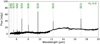 |
Fig. 1 MIRI MRS spectrum in an aperture extracted near knot A (see Figure C.2). The H2 0–0 S(1)–S(8) transition wavelengths are indicated with grey shading. The spectrum shows clear rotational H2 lines up to 0–0 S(7). |
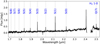 |
Fig. 2 NIRSpec spectrum extracted in an aperture 0′.′63 from the source, along the jet axis (see Figure C.1). The H2 1–0 S(0)–S(8) and 1–0 Q(7) transition wavelengths are indicated with grey shading. The 1–0 S(0)– S(5) and 1–0 Q(7) transitions are detected in this work. |
Laboratory wavelengths (λ) for the near-IR H2 transitions used in this work.
3 Results
We begin this section by describing the extraction of the emission line parameters and presenting the outflow morphology from integrated line flux maps. We map three outflow properties in 2D using the emission lines, namely the velocity, temperature, and ortho-to-para ratio (OPR). The mid- and near-IR emission lines and their wavelengths as used in this work are listed in Table 1 and Table 2 respectively.
3.1 Integrated line flux maps
3.1.1 Line fitting
To obtain velocity, temperature, and OPR maps we first measured the integrated flux and redshift of each line in each spaxel.
We locally subtracted the continuum using a quadratic spline fit. The continuum uncertainty around each emission line was estimated using a sampling methodology as described in Appendix A to take into account the bias introduced by manually picking continuum regions in the spectrum. A Gaussian curve was fit to the continuum subtracted spectrum in a 600 km s−1 wide region around the laboratory wavelength of each line to determine the line centroid and integrated flux. We rejected line fits with an amplitude smaller than 5σ in the mid-IR and near-IR line maps and 3σ in the near-IR apertures, with σ the uncertainty as follows from the continuum subtraction routine. The threshold for near-IR lines in apertures was lower as the fit quality within the apertures could be assessed manually. The line fitting routine was applied to the wavelength dimension of each spaxel in the data cube.
To obtain the poloidal velocity of the emitting H2 , one may subtract the systemic velocity υsys = 9.9 km s−1 (Dunham et al. 2014; Dutta et al. 2022) from the line centroid velocities and correct for the flow inclination angle of i = 40° (Chrysostomou et al. 2008; Dutta et al. 2022), if the flow is collimated. Therefore, we present corrected velocities υcorr for the 1–0 S(1) transition (measured in apertures), and do not present corrected velocities for the rotational transitions. There are two main sources of uncertainty for the rotational H2 velocities. Firstly, as the flow is not collimated, the observed velocity centroid in each spaxel contains contributions from streamlines with varying opening angles. The contribution of each component to the velocity vector differs per spaxel. Secondly, wavelength-dependent systemic wavelength corrections up to 90 km s−1 are required to reach 3–5 km s−1 rms in the MIRI MRS wavelength solution (Pontoppidan et al. 2024b). This is evident from our velocity maps, which show 10–30 km s−1 redshift in the blueshifted after correction for the systemic velocity and inclination for some transitions (see Figure C.3). We note that the instrumental corrections are not necessary to perform spaxel-by-spaxel comparisons of velocity, as the offset is only wavelength dependent. Therefore, we may study the velocity structure for each rotational transition separately, taking into account that we are measuring the contribution of streamlines with a range of opening angles.
3.1.2 Mid-IR line emission
Mid-IR molecular hydrogen lines are easily excited at low temperatures (300–1500 K) and densities (critical densities ≲106 cm−3 for the given temperature range), tracing the shocked gas and jets in outflow cavities (Le Bourlot et al. 1999; Lahuis et al. 2010).
Figure 1 shows an example of an MRS spectrum in the outflow. The H2 0–0 S(0) line is not detected at any position, as the spectra are too noisy around 26 µm. The S(1)–S(5) transitions are easily detectable, while the higher-J transitions are much weaker. The 0–0 S(1)–S(5) transitions are used to construct rotation diagrams, as these transitions are spatially resolved in the outflow.
We present the integrated flux map of 0–0 S(2) in Figure 3 (left), along with the extent of the 230 GHz 2–112 CO emission in the object as observed with ALMA (Dutta et al. 2022). The maps for the other mid-IR lines studied in this work can be found in Figure C.2. The blueshifted outflow lobe is detected spaxel-by- spaxel in S(1)–S(5) and S(7). The redshifted lobe is obscured by the protostellar envelope and does not show clear H2 emission features. The molecular hydrogen emission traces a wide-angled outflow from the protostellar object. It is confined within the extent of the 2–1 12CO emission. Integrated H2 fluxes are highest along the jet axis (indicated with a white dotted line in Figure 3).
The outflow opening angle is inversely proportional to Eu (Figure B.1) – more energetic material is more collimated – suggesting that the mid-infrared molecular hydrogen lines trace the disk wind of HOPS 315 (Tychoniec et al. 2024). For the methodology to measure the width of the outflow, see Appendix B.
Two knots are detected along the jet axis. Knot B is furthest from the source at approximately 3″ (1200 au – given the distance D ~ 400 pc; Zucker et al. 2019), while knot A is closer to the source at a distance of approximately 1′.′5 (600 au). Knot B is out of the field of view of MRS Channels 1 and 2.
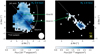 |
Fig. 3 Molecular hydrogen 0–0 S(2) (left) and 1–0 S(1) (right) integrated flux maps of HOPS 315. The maps are derived from Gaussian fits to the emission lines in each spaxel. Black spaxels indicate spaxels where no line with a peak continuum-subtracted flux >5σ was detected (where σ is the continuum uncertainty) or that are out of the image field of view. White circles illustrate the size of the PSF FWHM at the transition wavelength. The dotted line indicates the jet axis, originating from the source (grey star). Two flux peaks can be identified in the left image, labelled with knot A and B. The former is also visible in the right image. Left: the white contours show the collimated 1–0 S(1) emission. The dashed-line parabola indicates the extent of the 2–1 12CO emission (230 GHz) observed by Dutta et al. (2022). Right: the NIRSpec PSF is surrounded by a yellow box such that it is easier to spot. |
3.1.3 Near-IR line emission
At near-IR wavelengths, ro-vibrational H2 probes more collimated emission closer to the jet than mid-IR H2 (e.g., Davis et al. 2002), tracing dense, molecular gas at relatively more energetic conditions ( , T ~ 2000–3000 K).
Figure 2 shows an example of a NIRSpec IFU spectrum in the outflow. The 1–0 S(1)–S(5) lines are detectable, while higher-J transitions do not exceed the continuum noise. Therefore, we used the 1–0 S(1)–S(5) transitions to construct rotation diagrams.
The spatial distribution of 1–0 S(1) emission is shown in Figure 3. The H2 1–0 S(1) emission is collimated around the jet axis, as found in earlier observations of HOPS 315 presented in Davis et al. (2011) that led to its classification as small-scale H2 jet object. In contrast to the pure rotational lines, which disappear near the protostar, near-IR ro-vibrational emission is strongest near the protostar. In fact, the flux strongly falls off with distance from the source at distances ≳0′.′5. The intensity profile shows a small peak near the position of knot A, which was identified in the pure rotational transition maps. Knot B is not within field of view. More energetic lines in the 1–0 S branch are fainter and detected only in more limited spatial extent than S(1).
NIRSpec spaxel-by-spaxel analysis is complicated by the spatial undersampling of the PSF, which introduces low- frequency quasi-periodic flux fluctuations in the spectra (see e.g. Section 1.3 in Ruffio et al. 2024). This increases uncertainties on the line velocity centroids and integrated fluxes. The fluctuations can be reduced to <1% of the continuum flux in aperture-averaged spectra with a radius at least 1.5 times the PSF FWHM (Law et al. 2023). Recall that we extract apertures of radius 0′.′2 for NIRSpec data, while we measure a FWHM of approximately 0′.′1. We only present these aperture-averaged results for the near-IR H2 from this point forward.
3.2 Gas kinematics
The origin of the molecular hydrogen emission can be inferred from the radial velocity distributions of the respective lines. We summarised the 2D velocity map for each pure rotational line (shown in Figure C.3) by producing profiles along and perpendicular to the jet axis. The 2D maps were rotated by 47° to align the jet axis with the x-axis. We computed the median velocity along the x-axis (at each y-coordinate) to obtain the velocity profile perpendicular to the jet (Figure 4). The median velocity along the y-axis (at each x-coordinate) then yielded the velocity profile along the jet (Figure 5). Only columns in which at least five spaxels contain a line detection are included to reduce noise.
We did not produce near-IR molecular hydrogen line velocity maps due to the aforementioned distortion correction issues. Instead, we measured the velocity in several apertures along the jet axis using the 1–0 S(1) transition, which is the strongest H2 transition in the near-IR. The 1–0 S(1) velocity profile along the jet axis is shown in Figure 5. The ro-vibrational H2 shows acceleration from 35 km s−1 in an aperture centred on the protostar to 105 km s−1 at knot A. The exponential fit to the data implies a terminal velocity of 120 km s−1 (indicated with a dashed grey line in Figure 5), with ~15 km s−1 uncertainty.
We observe two trends from the velocity distributions: (1) molecular hydrogen emission nearer to the jet axis is more blueshifted; (2) material further from the source is more blueshifted. Figures 4 and 5 respectively illustrate trends (1) and (2). These trends are interpreted in Section 4.2.
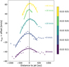 |
Fig. 4 Radial velocity υrad profile perpendicular to the jet axis for 00 S(1)–S(5). Positive values correspond to blueshift. Each datapoint is the median radial velocity along the spaxel column of the rotated image (see Section 3.2). The solid curves are second-order polynomial fits to the data. The curves are offset for clarity. The offset for each curve is annotated in the figure in the same colour. |
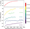 |
Fig. 5 Corrected (1–0 S(1), top) and radial (0–0 S(1)–S(5), bottom) velocity profiles, respectively υcor and υrad . Positive velocity values correspond to blueshift. Each datapoint in the pure rotational molecular hydrogen curves is the median velocity along the spaxel column of the rotated image, while the 1–0 S(1) curve is derived from several apertures along the jet axis (see Section 3.2). The solid curves are exponential fits to the data. The rotational transition curves are offset for clarity. The offset for each curve is annotated in the figure in the same colour. |
3.3 Temperature and column density
3.3.1 Rotation diagrams
Using the previously obtained line flux maps, we derive the rotational temperature and column density of the emitting molecular hydrogen gas from rotation diagrams. We construct the rotation diagrams from the 0-0 S(1) to S(5) lines for MIRI and 1–0 S(0)–S(5) lines for NIRSpec. We assume optically thin radiation, valid even for  (Bitner et al. 2008; Neufeld et al. 2009), which is orders of magnitude higher than typically measured in protostellar environments. The upper state column density Nu is then calculated from the integrated line flux Fint adopting
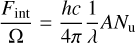 (2)
(2)
where λ is the wavelength of the emission line, Ω is the solid angle of the emitting area and A is the Einstein A coefficient of the transition. The value of Ω depends on the methodology we adopt to merge channel data. In the case of aperture extraction, the emitting area is the solid angle of the aperture, while in the case of spaxel-by-spaxel analysis, Ω is the solid angle of a spaxel.
The temperature and total column density are obtained from a Boltzmann distribution fit to the upper state column density data, assuming local thermal equilibrium (LTE). The assumption of LTE is supported by the low values of the critical densities for the pure rotational transitions (see Section 3.1.2), and is validated by assessment of the quality of the rotation diagram fits. The necessary transition parameters (degeneracies and Einstein A) and the total partition function are taken from the HITRAN database (Laraia et al. 2011; Gordon et al. 2022).
3.3.2 MIRI rotation diagrams
The temperature map resulting from rotation diagram fits to the 0–0 S(1)–S(5) transitions is presented in Figure 6, along with an example of a fit. Only spaxels are presented that are within the extent of the 0–0 S(4) emission, as the spatial extent of its integrated flux map is smallest of the five transitions (Figure C.2). A single temperature component is sufficient to describe the S(1)– S(5) rotation diagrams. The data follows a straight line in the extent of the mapped area, validating our assumption of LTE and implying that the ortho-to-para ratio is close or equal to 3.
Temperatures in the outflow range between 500 and 600 K (typical uncertainties 10 K). Interestingly, while knots are commonly associated with local temperature maxima (e.g., Nisini et al. 2010; Giannini et al. 2011), knot A does not exhibit temperature enhancement.
3.3.3 NIRSpec rotation diagrams
We produced near-IR rotation diagrams for three apertures along the jet in which we were able to detect six ro-vibrational lines, 1–0 S(0) to S(5) (Figure 7). The aperture locations are indicated in Figure C.1 and placed at distances of 0′.′34, 0′.′63 and 0′.′78 along the jet axis. We refer to these apertures as AP1, AP2 and AP3 respectively. The temperatures, column densities, and OPRs resulting from the rotation diagrams are listed in Table 3. The ro- vibrational emission probes hot gas T = 2400 − 3800 K, while the pure rotational H2 lines probe warm gas T = 500−600 K.
Recall that a zigzag pattern is observed in H2 rotation diagrams when OPR < 3, as the even-J (para-H2) transitions are systematically offset to higher ln (Nu /gu). Figure 7 illustrates that the OPR drops below 3, decreasing further from the source. The equilibrium OPR at temperatures T > 300K is 3 (Burton et al. 1992). At a temperature T ~ 3000 K, we measure OPR < 3. The near-IR emission thus probes gas in ortho-to-para disequilibrium.
To estimate the uncertainty on the OPR, we must consider its covariance with each source of uncertainty. For example, the variance in extinction (AK) predominantly affects the column density and rotational temperature and does not have a strong influence on the OPR. This is illustrated in Figure 8, where the results for three different values of AK are plotted for each aperture. The OPR is relatively unaffected by the variance in AK , while the slope (temperature) and magnitude of ln Nu/gu (column density) vary noticeably. We used a sampling procedure to propagate the uncertainties, as it accounts for the covariance between fitting parameters and each source of uncertainty. This sampling procedure was not required for the mid-IR rotation diagrams, as these are less strongly affected by variance in extinction – see Section 4.1.
The sampling procedure was implemented as follows. First, we drew 300 samples from a Gaussian distribution for AK (recall AK ≈ 2.9 ± 0.4 mag) and corrected the spectra for extinction as described in Section 2.3. For each line in each of these spectra, we found the integrated flux F and its uncertainty σF , which is a combination of uncertainty from Gaussian fitting and continuum uncertainty. This led to a single set of six (Eu, ln (Nu/gu)) pairs for each extinction value – three examples are shown in Figure 8. Next, we drew 100 samples from a Gaussian distribution with mean F and width σF for each transition. We fit a rotation diagram to each set of transitions (as shown with lines in Figure 8) and calculated the mean T, N, and OPR of the 100 fits, yielding a single measurement for the three parameters for a given AK. The 50th, 84th, and 16th percentiles of those 300 separate measurements with varying AK are reported in Table 3.
We find that the OPR is significantly lower than 3 in AP2 and AP3, equal to 2.71 ± 0.02 and 2.49 ± 0.03 respectively. Contrastingly, the OPR is equal to 3 closer to the source (AP1). We interpret these results and discuss the influence of additional sources of uncertainty on their significance in Section 4.4.
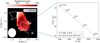 |
Fig. 6 0–0 S(l)–S(5) temperature map as derived from 0–0 S(l)–S(5) rotation diagrams. Left: the temperature map, with white contours derived from 0–0 S(2) emission outlining the positions of knot A and B. The white circle indicates the PSF FWHM that each transition integrated flux map has been smoothed to. Right: example of a single-spaxel rotation diagram. The measurements follow a straight line characterised by the temperature T and column density N as indicated in the grey box. |
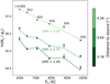 |
Fig. 7 Rotation diagrams for ro-vibrational H2 emission in three apertures at various distances (in the image plane) from the source. The ortho-to-para ratio (OPR) decreases further from the source. The temperature and column density corresponding to each fit are listed in Table 3. Plotted uncertainties do not include the extinction uncertainty, which affects each curve as illustrated in Figure 8. |
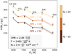 |
Fig. 8 Rotation diagrams for ro-vibrational H2 emission in an aperture at 0′.′78 from the source (AP3), adopting three different values for the extinction AK . Fit parameter medians and uncertainties listed in the shaded box are derived using a sampling procedure (see Section 3.3.3). 100 sampled Boltzmann distribution fits are plotted for three different values of AK to portray its influence on the best-fit ortho-to-para ratio (OPR). |

4 Discussion
In this section, we interpret the results presented in the previous section. The rotational H2 emission exhibits characteristics best described by magneto-hydrodynamic (MHD) disk wind models, while the ro-vibrational H2 emission likely probes HOPS 315’s molecular jet. In Section 4.1 we describe the effect of the assumption of constant extinction on our results. In Section 4.2, we compare our observations to MHD disk wind models and past observations. Next, we compare the ro-vibrational H2 properties to those of jet launching models in Section 4.3. Lastly, in Section 4.4, we propose potential explanations for the observed ortho-to-para disequilibrium in ro-vibrational H2 , in contrast to the equilibrium ratio we measure in rotational H2.
4.1 Extinction
We assumed a constant extinction value throughout the image, derived from the 1–0 S(5) and 1−0 Q(7) H2 line ratio measured in AP2. However, the extinction might vary along the outflow (see e.g., Narang et al. 2024; Delabrosse et al. 2024; Caratti o Garatti et al. 2024), decreasing with distance from the protostar. Extinction measurements are often made using rotational H2 rotation diagrams (Dionatos et al. 2010; Davis et al. 2011; Narang et al. 2024; Tychoniec et al. 2024) or line ratios (Caratti o Garatti et al. 2006; Davis et al. 2011; Melnikov et al. 2023b; Delabrosse et al. 2024; Caratti o Garatti et al. 2024).
The H2 rotation diagram approach assumes that H2 is in LTE and that OPR = 3, measuring the extinction based on the variance of the data around the straight line fit (in the case of one temperature component). However, non-thermal effects (such as additional temperature components) and OPR < 3 also lead to deviations from the straight line fit. Fitting the extinction, temperature, column density, and OPR based on five datapoints – 0–0 S(1)-S(5) – would lead to a fitting parameter degeneracy problem. The scatter around the straight line might be caused by OPR < 3, non-thermal effects, or extinction. As we aimed to test the assumptions of OPR = 3 and LTE, we did not to use the rotational H2 rotation diagrams to derive extinction.
Alternatively, ratios of near-IR H2 or [FeII] lines are commonly used to measure extinction. We were unable to apply these methods in our work to map the extinction along the outflow. The necessary transitions either fall in the NIRSpec detector gap (in particular the low-J lines of the 1−0 Q branch of H2 near 2.4 µm, see Figure 2) or are not detected in this source along the outflow.
To estimate impact of the constant extinction assumption, we first consider the magnitude of the potential decrease of extinction along the outflow. Narang et al. (2024) report a decrease from AV = 27 to AV = 24 on a scale of 4″ in the Class 0 source IRAS 16253-2429. Delabrosse et al. (2024) report a decrease of AV = 15 mag to AV ~ 0 mag on a scale of 600 au in the Class I source DG Tau B. Recall that we have adopted the constant value AV = 26 ± 4 mag. The decrease measured by Narang et al. (2024) therefore falls within our uncertainty, while that measured by Delabrosse et al. (2024) is significantly larger. The extinction uncertainty dominates each parameter’s uncertainty (disregarding unknown systemic uncertainties), with the exception of the OPR and radial velocities. Therefore, we can use the uncertainties we have derived to illustrate the impact of variance in extinction.
The mid-IR H2 rotation diagrams are not strongly affected by extinction. We likely overestimated the mid-IR rotation diagram uncertainties in our approach (disregarding unknown systemic uncertainties), as we did not apply a sampling procedure, such as was done for the ro-vibrational H2 rotation diagrams. Despite this, the uncertainty in rotational H2 temperature is ∼10 K. The marginal influence of mid-IR extinction on the rotational H2 temperature as observed in our work was also noted in Giannini et al. (2011); Melnikov et al. (2023a); Gieser et al. (2023). Column density is more strongly affected by extinction uncertainty. Therefore, the column density measurements likely have higher uncertainty than reported in our work as a result of the assumption of constant extinction. In contrast to rotational H2 , the ro-vibrational H2 temperature and column density are highly uncertain as a result of extinction uncertainty (see Table 3 and Figure 8). Importantly, recall that we observed that variance in extinction does not significantly affect the OPR (see Section 3.3.3). Therefore, we conclude that the assumption of a constant extinction across the outflow leads to additional uncertainty in near-IR column density and temperature measurements, and mid-IR column density measurements. In particular, the observed decrease in ro-vibrational H2 column density is potentially a consequence of the assumption of constant extinction.
Lastly, we consider the impact of the constant extinction assumption on the measurement of OPR < 3 in the jet. If there were a strong correlation between extinction and OPR, it would be observable in Figure 8. The sampled rotation diagrams in this figure show a weak apparent increase in OPR with decreasing extinction. This apparent trend is likely a consequence of the randomness of the sampling technique. We drew a limited number of rotation diagram samples (100) per Ak value to reduce the runtime of the sampling algorithm. While this is sufficient to yield a consistent median OPR across sampling runs (recall that we found the median from 300 sampled Ak values each with 100 sampled rotation diagrams), OPR measurements for a given sampled Ak can vary across different instances of the sampling algorithm. The uncertainty on each separate OPR measurement per Ak in Figure 8 is approximately 0.1 as a result of limited sampling – the differences between the measurements are therefore not significant. Rerunning the sampling would randomly produce figures with a reversed apparent trend to the one in Figure 8, or often produce no apparent trend at all, as a result of small number statistics – we only plot three values of extinction in the figure. In the full sample of 300 Ak values, we do not detect any correlation with OPR. Therefore, we conclude that the assumption of constant extinction does not affect the significance of the result that OPR < 3 in AP2 and AP3.
Results of the rotation diagram fits to 1−0 S(0)–S(5) emission in three different apertures. The position of each aperture is indicated in Figure C.1. The distance (d) to the protostar in the image plane, ortho-to-para ratio (OPR), temperature (T) and column density (N) are listed for each aperture. The uncertainties are derived as described in Section 3.3.3.
4.2 Origin of the rotational emission
There are various potential origins for the observed rotational H2 emission. The emission could trace an MHD disk wind, which are magnetically launched from a range of wind ejection footpoint (base) radii r0 . Alternatively, the emission may trace a photoevaporative wind, which would be thermally driven by (far ultraviolet, extreme ultraviolet or X-ray) photons. While pho- toevaporative winds are not usually thought to be effective in Class 0 and I objects, as the high-energy radiation must be able to penetrate in the wind to drive it on large scales, recent work indicates molecules may survive in them (Sellek et al. 2024). We note that conclusions from these models may not be directly applicable to HOPS 315, as they have been developed for the later Class II stage, while HOPS 315 is a young Class I source. Additionally, we may trace entrained ambient material driven by fast stellar winds, also known as the ‘wide-angle wind driven shell model’ (Li & Shu 1996; Lee et al. 2000). Similarly, jet bow shocks may entrain ambient material or the disk wind (Tabone et al. 2018; Rabenanahary et al. 2022). In this section, we compare our observations with the observational signatures these different scenarios predict.
Morphologically, we observe a wide-angled outflow from the source that is increasingly collimated in transitions with higher upper state energy Eu (Figure B.1). This relation between the outflow opening angle and Eu is also observed in TMC1-W (Tychoniec et al. 2024), where it is interpreted as a sign that the rotational H2 traces an MHD disk wind. In MHD disk winds, material at larger footpoint radii produces larger outflow opening angles (Matt & Pudritz 2005; Tabone et al. 2020). In this scenario, the higher Eu transitions would trace material launched from smaller r0 . In general, the increasing collimation of higher Eu transitions is a sign of radial stratification in excitation conditions. This is expected for MHD disk wind and photoevaporative wind models (Komaki et al. 2021; Pascucci et al. 2023), where hotter material can be found closer to the flow axis. We note that an increase in rotational H2 temperature (derived from 0–0 S(1)- S(5) transitions) towards the flow axis is not clearly observed in our work, see Figure 6.
We observe two velocity trends in the outflow. The first is a decrease in velocity with distance across the outflow axis (Figure 4). A velocity decrease with distance from the outflow axis is commonly observed in T Tauri jets and was also observed previously in the H2 jet of HOPS 315 (Chrysostomou et al. 2008). This suggests radial stratification of velocity. However, projection effects in velocity structure due to the range of streamline opening angles may affect the observed velocity stratification in wide-angled flows. These would need to be taken into account to retrieve the true kinematics of the flow. A decrease in velocity across the outflow axis is produced in MHD disk winds, pho- toevaporative winds, and the jet bow shock driven model, but not in traditional wide angle wind driven shell models. In an MHD disk wind of uniform magnetic level arm, the poloidal velocity is proportional to the Keplerian velocity at the streamline footpoint radius. Material from inner streamlines has higher Keplerian speeds. Hence, material closer to the outflow axis has higher poloidal velocities as it is launched (Blandford & Payne 1982; Anderson et al. 2003; Ferreira et al. 2006). In the jet bow shock driven model, the decrease in velocity is a result of deceleration of bow shock wings that expand and interact inside the shell (Rabenanahary et al. 2022). Photoevaporative winds also predict a decrease of flow velocity across the outflow axis (e.g., Komaki et al. 2021). On the other hand, traditional wide-angle wind driven shell models produce elliptical contours in transverse position-velocity diagrams, which do not correspond to a decrease in velocity with distance from the flow axis (Lee et al. 2000). However, a stacking of wind driven shells resulting from a variable inner wind may produce a decrease in velocity across the flow axis. In this scenario, the outer shells would have lower velocities (Zhang et al. 2019).
Secondly, we observe acceleration along the outflow axis (Figure 5). Material in the outflow is accelerated out to ∼1500 au. Long-range (distances ≳ 1000 au) acceleration was previously measured in the molecular flows of HH 212 (Lee et al. 2022) and Cep E (Schutzer et al. 2022). Linear (‘Hubble law’) acceleration along the outflow axis is predicted in the wind-driven shell model, assuming the density ρ of the ambient material scales as ρ ∝ sin2 θ/r2 (with θ the polar angle from the outflow axis, r the distance from the protostar) (Lee et al. 2000). Assuming identical density scaling, the jet bow shock driven model can also produce a Hubble law acceleration, or a sawtooth pattern caused by bow shocks of individual outflow bullets (Rohde et al. 2019; Rabenanahary et al. 2022). MHD disk wind ejection models also predict that poloidal velocities increase with distance from their launching point. The velocity profile flattens at distances in the order of ∼100 r0 for the λ ∼ 5–13 models (λ refers to the magnetic lever arm) of Bai et al. (2016) and Tabone et al. (2020).
Lastly, models must be able to account for emitting H2 moving at flow velocities υ ≳ 20 km s−1 – consider that if the minimum velocity measured for each transition corresponds to υ ≥ 0km s−1, velocities ≳20 km s−1 are reached since the velocity trends along and across the outflow axis show acceleration of this order. Molecular material moving at velocities υ ≳ 20 km s−1 are incompatible with current photoevaporative wind models. Photoevaporative wind models struggle to account for molecular flows at high velocities, predicting molecular flows below 10km s−1 (Komaki et al. 2021).
We conclude that a photoevaporative origin of the H2 emission in HOPS 315 is unlikely, based on the opening angle of the outflow and the presence of υ ≳ 20 km s−1 molecular flows. More detailed kinematics of the wide-angled flow, in particular an attempt to measure the potential rotation of the outflow, might be used to further contrast the different potential origins of the H2 emission. As we do not observe any clear, consistent asymmetry in the velocity profile across the outflow axis, we estimate that a rotation signature would be weak (υϕ ≲ 10 km s−1).
4.3 Origin of the inner jet
Rotational H2 emission is enhanced along the jet axis of HOPS 315, while ro-vibrational H2 emission is only observed in closely collimated around the jet axis, indicating the presence of an H2 molecular jet in the outflow. Conversely, protostellar objects with atomic jets predominantly show V-shaped rotational and ro- vibrational H2 emission, tracing shocks filling the outflow cavity wall – see recent work with NIRSpec IFU and MIRI MRS data such as Yang et al. (2022); Harsono et al. (2023); Federman et al. (2024); Arulanantham et al. (2024); Tychoniec et al. (2024); Delabrosse et al. (2024); Nisini et al. (2024). No atomic or ionic emission is observed in the HOPS 315 outflow – studies of [FeII], [SII], and [OI] showed no emission in the jet (Antoniucci et al. 2008; Davis et al. 2011; Sperling et al. 2020).
We measure a temperature of 2400–3800 K for the emitting ro-vibrational H2 in the molecular jet of HOPS 315. Previously, temperatures of 2350–3500 K (Caratti o Garatti et al. 2006) and 3000 K (Davis et al. 2011) were measured for ro-vibrational H2 emission in the molecular jet of HOPS 315. The observed range of temperatures for ro-vibrational H2 across all environments is limited as the molecule is collisionally dissociated for temperatures ≳3000 K, but is not excited at lower temperatures (Pascucci et al. 2023). Our observations are in line with the limited temperature range expected for ro-vibrational H2 emission. Atomic jets, on the other hand, can reach higher temperatures (∼10 000 K).
The velocity of hot H2 gas is higher than the warm (rotationally emitting) gas. We measure gas speeds up to 105 km s−1 in the hot gas at 1″.5 from the protostar using H2 1−0 S(1) emission. This is within the range of typical Class 0 jets speeds of 100 ± 50km s−1 (Jhan & Lee 2015; Podio et al. 2016; Yoshida et al. 2021; Pascucci et al. 2023). In contrast, ro-vibrational H2 has V-shaped morphology in sources with atomic jets, tracing material with velocities <30km s−1 (Agra-Amboage et al. 2014; Melnikov et al. 2023b; Federman et al. 2024; Delabrosse et al. 2024).
Chrysostomou et al. (2008) found ajet velocity of 110 km s−1 from H2 1−0 S(1) emission in HOPS 315 at 2″ from the protostar. Moreover, Dutta et al. (2022) measure a mean jet velocity of 125 km s−1 from CO and SiO emission on a scale of ∼10″. These measurements are consistent with the exponential velocity profile we observe for 1−0 S(1) in Figure 5. The velocity profile flattens at ∼1500 au from the protostar, reaching a terminal velocity of 120–125 km s−1. In steady and cold MHD disk winds, the terminal velocity of the streamline Vp,∞ is approximately
 (3)
(3)
where Vkep(r0) refers to the Keplerian velocity at r0 (see Fig. B.1 in Jacquemin-Ide et al. 2019). Therefore, the acceleration we observe would require λ > 28 if we adopt r0 ≈ 2–4 au for the jet of HOPS 315, as estimated from tentative rotation signatures by Chrysostomou et al. (2008) and the mass M ≈ 0.6 M⊙ (Antoniucci et al. 2008). Current MHD ejection models may struggle to explain large-scale jet acceleration as noted by Lee et al. (2022), who recommended further work to check if other effects such as time variability in the ejection velocity and geometrical projection can produce this apparent acceleration.
It is possible that the jet is launched by the same mechanism as the wind. The acceleration pattern observed from 1−0 S(1) emission is similar to that of the rotational transitions. The opening angle decreases for higher Eu transitions in the mid-IR. The 1−0 S(1) emission has higher Eu than 0–0 S(1)- S(5) and is indeed more collimated. Moreover, the velocity and temperature of the H2 jet are higher than the wide-angled rotationally emitting H2. Such nested morphology is a distinctive characteristic of MHD disk winds and is observed by Tychoniec et al. (2024). The ro-vibrational H2 jet may then trace material launched from streamlines closer to the protostar than the rotational H2 disk wind. However, because we do not detect high-energy rotational transitions (0–0 S(6) and higher) on large scales, there is a significant gap between the rotational and ro- vibrational lines in this work. Moreover, we are unable to test if the flow velocity gradually increases for higher Eu transitions up to the jet velocity as a result of MIRI MRS calibration uncertainties. Studying the higher rotational transitions and the absolute velocities of the rotational transitions may further constrain the possibility that there is a smooth transition from the wide-angled H2 wind to the collimated H2 jet.
4.4 Ortho-to-para disequilibrium
We measure a decrease of the OPR in the jet from its equilibrium value of 3 in API (200 au) to 2.49 ± 0.03 in AP3 (500 au). Conversely, the rotational H2 emission probes gas with OPR = 3 in the extent of the mapped area.
4.4.1 Additional uncertainties
Additional sources of uncertainty may impact the significance of the measurement of OPR < 3 in the jet. Our uncertainty estimation cannot account for the variance observed in the rotation diagram of AP1, where OPR = 3 (Figure 7). One source of uncertainty not included in our uncertainty estimation is the choice of extinction curve. The shape of the extinction curve affects the relative offset of respective states. Adopting the KP v05 extinction curve (Chapman et al. 2008; Pontoppidan et al. 2024a) – which appears to be more suitable for dereddening the H2 lines (Narang et al. 2024) – instead of the McClure (2009) curve did not affect results. In both extinction curves, extinction decreases monotonically in the 1−0 S(0)–S(5) wavelength range, which does not affect the zigzag pattern. Thus, extinction curve uncertainty is unlikely to impact the result’s significance, but the variance in the AP1 rotation diagram suggests additional uncertainties we have not accounted for.
Moreover, the excitation mechanism may cause a discrepancy between the observed OPR in rotation diagrams and the bulk ortho-to-para abundance ratio. In previous work, observed ro-vibrational OPR lower than 3 in rotation diagrams of photon- dominated regions has been misinterpreted as gas in ortho-topara disequilibrium, when in fact the observed OPR reflected optical depth effects due to far-ultraviolet pumping (Black & van Dishoeck 1987; Sternberg & Neufeld 1999). However, if we assume that the ro-vibrational H2 is shock-excited in HOPS 315 (as is expected for Class I MHEL regions; Davis et al. 2011), the OPR in ro-vibrational H2 rotation diagrams reflects the bulk H2 ortho-to-para abundance in its jet (Sternberg & Neufeld 1999).
4.4.2 Physical interpretation
A mismatch between the expected OPR in LTE (OPRLTE) at a given temperature and the observed OPR (OPRobs) is commonly found in shock-excited regions. In these environments OPRobs < OPRLTE, which was previously interpreted as a remnant of earlier epochs (Maret et al. 2009; Nisini et al. 2010; Giannini et al. 2011; Neufeld et al. 2006, 2009, 2019). Cool, preshock gas with a temperature T < 300 K equilibrates to lower OPR. When a shock elevates the gas temperature, the OPR is raised to the higher-temperature OPRLTE over a timescale τ. Consequently, OPRobs < OPRLTE is observed when the gas has been excited to the higher temperature for a time t < τ.
The timescale to reach ortho-to-para equilibrium depends strongly on environmental parameters, such as the temperature, density, and dominant ortho-to-para conversion reaction. In nondissociative molecular shocks, the dominant para-to-ortho conversion reaction is assumed to be reactive collisions with atomic hydrogen (Timmermann 1998; Wilgenbus et al. 2000). This reaction has a strong temperature dependence due to its high activation energy E/kB ~ 4000 K. If ortho-to-para conversion through reactive collisions with atomic hydrogen dominates, the timescale to reach OPRLTE depends on the para-ortho conversion rate kpo = exp (−3900/T) ⋅ 8 × 10⁻¹¹ cm3 s−1 (Schulz & Le Roy 1965; Schofield 1967) and atomic hydrogen number density n(H) as
 (4)
(4)
regardless of the pre-shock OPR (where we approximated 1 – e−3 ≈ 1) (Neufeld et al. 2006). Measurements of n(H) in Class 0/I sources indicate n(H) ≈ 103–104 cm−3 (Maret et al. 2009; Nisini et al. 2010; Giannini et al. 2011), measured simultaneously in the warm and hot components of outflows. This yields equilibration timescales of τ ≈ 0.5–5 yr for the hot gas, and τ ≈ 80–800 yr for the warm gas.
Evidently, hotter gas equilibrates faster when reactive collisions with H dominate para-ortho conversion. Under these conditions, if the pre-shock OPR, pre-shock n(H), and the time since excitation are the same, we must then always find higher OPR in hotter gases. Previous observations of the OPR in protostellar outflows indeed found higher OPR in warmer regions (Neufeld et al. 2006, 2009, 2019; Maret et al. 2009; Nisini et al. 2010; Giannini et al. 2011). Contrary to these observations, we observe OPRwarm > OPRHot. We propose several potential explanations for our results below.
Previous work has assumed that reactive collisions with atomic hydrogen dominate ortho-to-para conversion, which raises the OPR. Alternative ortho-to-para conversion reactions in the gas phase or on grain surfaces may lower the OPR. In the gas phase, proton exchange reactions with  and H+ can lower the OPR. However, these reactions influence the OPR only on timescales of 106 yr, which is orders of magnitude larger than the dynamical timescale of the jet (500 au/100km s−1 ≈ 25 yr). Moreover, these reactions dominate only at low temperatures (≲30 K; Flower et al. 2006; Lique et al. 2014). We conclude that alternative gas phase reactions are unlikely to lower the OPR in the jet.
The effect of grain surface reactions on the OPR is more complicated. Grain surface reactions were previously used by Shinn et al. (2012) to explain the measurement of nonequilibrium OPR in supernova remnants with near-IR molecular hydrogen lines. The formation of H2 on grain surfaces is typically assumed to yield OPR = 3 due to the exothermicity of the formation reaction, but this is still uncertain as experimental work has been inconclusive (Takahashi 2001; Morisset et al. 2005; Pagani et al. 2009; Gavilan et al. 2012; Fukutani & Sugimoto 2013; Lique et al. 2014; Bron et al. 2016). After formation, the OPR may be lowered by ortho-to-para conversion on dust surfaces (Tielens & Allamandola 1987; Le Bourlot 2000; Fukutani & Sugimoto 2013; Bron et al. 2016). In particular, the OPR could be lowered efficiently on magnetised grains (Fukutani & Sugimoto 2013). Magnetised grains may form in the inner disk, where magnetic fields are strong (Fu et al. 2014; Wang et al. 2017) – recall that jets are launched magnetically (e.g., Pelletier & Pudritz 1992; Frank et al. 2014). Inner streamlines are more strongly magnetised. In the case of MHD disk wind launching, ortho-to-para conversion on magnetised grains in the inner disk might explain the equilibrium OPR in the disk wind in contrast to the disequilibrium OPR in the jet. The low-OPR, condensed H2 would likely be released into the gas phase in the jet rather than in the disk as equilibration timescales (~0.5–5 yr) are shorter than dynamical timescales (∼25 yr) in the jet. A more detailed investigation of (magnetised) dust grain ortho-to-para conversion and required magnetic field strengths for conversion is needed to understand if they may efficiently lower the OPR in protostellar environments.
Ortho-to-para conversion in the inner disk is also favoured over conversion in the jet based on dust sublimation temperatures. Dust sublimation for most species occurs around 1300– 1700 K (Lodders 2003). If the dust temperature is coupled to the gas temperature (T = 2400–3800 K in the H2 jet), dust is likely sublimated in the jet. In this scenario, grain surface reactions cannot occur in the jet. Instead, grain surface reactions could take place in the disk outside or near the dust sublimation radius. Dutta et al. (2022) estimate a dust mass ratio of 10−3 from the ratio of SiO and CO abundances, suggesting that the jet of HOPS 315 is possibly launched from dust-poor regions of the inner disk, either within the dust sublimation radius or from layers of the disk which have experienced gravitational removal of dust to the disk midplane (‘settling’). In contrast, the disk wind would extend over several hundred au in radius, consistent with the theoretical suggestion that the wind could be an effective means of redistributing hot dust from 1 au to the comet-forming regions of disks around 40 au at this age (Giacalone et al. 2019). Future studies could investigate the dust mass ratio required in the inner disk to efficiently lower the OPR.
Our results highlight the importance of continued work on theoretical and experimental studies of ortho-to-para conversion reactions on grain surfaces. Moreover, it will be valuable to study the H2 OPR in the molecular jets of other protostars to provide insight on ortho-to-para conversion mechanisms at high temperatures in circumstellar disks and protostellar outflows.
5 Conclusion
We mapped the molecular hydrogen emission of the HOPS 315 outflow in the near- and mid-IR using the NIRSpec IFU and MIRI MRS. We reveal the morphology, kinematics, temperature and OPR of the molecular hydrogen jet and disk wind. Our results and their interpretations are summarised as follows:
The rotational H2 transitions 0–0 S(1)–S(5) trace a wideangled wind component, extending radially to the cometforming regions of the disk at velocities ≳20 km s−1 and temperatures of 500–600 K;
The velocity of the rotationally emitting H2 increases towards the jet axis, increases with distance from the source, and the outflow is more collimated for lower Eu transitions. This is compatible with MHD disk wind launching theory, but may also be indicative of wide-angled wind- or jet bow shock-driven flows;
The ro-vibrational H2 transitions 1−0 S(0)–S(5) probe the molecular jet of HOPS 315. The emission is collimated around the jet axis, with a terminal velocity of 120– 125 km s−1 for 1−0 S(1) and a temperature of 2400–3800 K;
The rotational H2 is in ortho-to-para equilibrium at the given temperature (OPR = 3), while the ro-vibrational emission shows a decreasing OPR from 3 at 150 au to OPR = 2.49 ± 0.03 at a deprojected distance 500 au from the protostar;
The decrease in OPR in the high temperature jet with respect to the colder wind is in contrast with previous studies of the OPR in protostellar outflows at lower temperature regimes. The disequilibrium OPR in the jet may be the result of grain surface ortho-to-para conversion reactions in the inner disk. Future studies could investigate the dust mass ratio required in the disk to efficiently lower the OPR. Alternatively, additional observations of the OPR in hot protostellar H2 jets could constrain the conditions under which disequilibrium OPR in jets is observed.
Our work demonstrates the value of combining near- and mid- IR data to reveal the layered structure of protostellar outflows. JWST NIRSpec IFU and MIRI MRS data can be used to spatially resolve the kinematics and temperature structure of the H2 emission in the jet and disk wind of Class 0/I sources, allowing us to constrain their launching mechanisms.
Acknowledgements
We would like to thank Tracy Beck, John Black, Ewine van Dishoeck, Logan Francis, Caroline Gieser, Wout Goesaert, Lars Reems and Łukasz Tychoniec for helpful scientific discussions, and the anonymous referee for their insightful comments.
Appendix A Continuum uncertainty estimation
The continuum was estimated as a quadratic spline through several (6–8, depending on the transition) manually defined spectral bins surrounding the line (anchor points). A second-order spline was found to describe the smooth continuum well and lead to more cautious continuum fit uncertainties than a first-order spline.
The choice of anchor points influences the resulting continuum fit, and consequently also the integrated flux of the spectral line. Therefore, we applied a sampling procedure to estimate the uncertainty on the continuum fit. Crucially, this technique also measured the uncertainty introduced by manually selecting anchor points. The results of this technique are shown in Figure A.1.
The sampling technique was implemented as follows. First, we interpolated (to second order) the spectrum between the wavelength bins such that the spectrum was continuous. We randomly sampled anchor points from a Gaussian distribution centred on a manually defined anchor point and a standard deviation of 1.5 wavelength bins. The sampled anchor points are seen as black circles in Figure A.1, where more opaque regions contain more samples. 100 different sets of anchor points were drawn for each emission line. We found the quadratic spline through each set of anchor points, yielding 100 sampled continuum fits (green lines in Figure A.1). Finally, we obtained the uncertainty on the continuum fit per bin from the distribution of continuum fits. We estimated the uncertainty on the continuum fit σ as Gaussian. σ is the average of F84−F50 and F16–F50 where Fn denotes the nth percentile flux F of the continuum values in a wavelength bin. The resulting 1σ uncertainty on the continuum fit is shown in the bottom panel of Figure A.1.
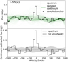 |
Fig. A.1 Example of a continuum fit and the estimation of its uncertainty for the near-infrared 1−0 S(4) line in AP2 (see Figure C.1). Top: The green lines indicate quadratic spline continuum fits through the sampled black anchor points. Only one in 30 sampled anchor points are shown for clarity. More opaque black or green colouring can be interpreted as a higher density of anchor points or continuum fits respectively. Bottom: The continuum-subtracted spectrum is plotted. The shaded area indicates the 1σ uncertainty of the continuum fits in each spectral bin. |
Appendix B Outflow width
We measured outflow width by fitting Gaussians to the line intensity maps, across the jet axis. The maps were rotated as described in Section 3.2, after which we performed Gaussian fits along the y-axis. The FWHM of the Gaussian profile in the data is determined by instrumental broadening and the width of the outflow. We approximated the width of the outflow as  where W denotes the FWHM of the outflow, Gaussian fit to the data and the instrumental PSF FWHM respectively. The intensity profiles across the jet axis are well approximated by a single Gaussian. We performed this fitting routine for the 0–0 S(1), S(2), S(3) and S(5) transitions as they are resolved in the outflow across the jet axis.
Next, we fit a straight line to WwidtH as function of the deprojected distance along the flow axis z and found its x-intercept xfit . For the 0–0 S(5) transition, the straight line was fit only to the first 6 datapoints, as the width profile appears to flatten for larger offsets (see Figure B.1). The opening angle spanned by the FWHM of the intensity profile is then
 (B.1)
(B.1)
where xfit accounts for the fact that the width of the outflow is nonzero at zero offset. The results are presented in Figure B.1.
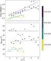 |
Fig. B.1 Opening angle and width as function of deprojected distance z for four rotational H2 transitions. Top: flow FWHM as function of z for each transition. The straight line fits used to correct the opening angle formula (Equation B.1) are indicated with dashed lines. Bottom: outflow opening angles θFWHM spanned by the FWHM of the flow intensity profile as function of z for each transition. Straight line fits to the data for each transition are shown to guide the eye. |
Appendix C 2D maps
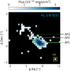 |
Fig. C.1 Continuum subtracted integrated flux map for the near-infrared transition 1−0 S(1). The grey star indicates the position of the protostar. The apertures used to construct rotation diagrams are indicated with green circles, where AP2 corresponds to the spectrum plotted in Figure 2. Each coloured spaxel corresponds to a Gaussian fit with a peak height larger than 5σ, with σ indicating the uncertainty on the continuum flux as described in Appendix A. The white circle in the bottom right indicates the PSF FWHM at the transition wavelength. |
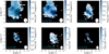 |
Fig. C.2 Continuum subtracted integrated flux maps for the mid-infrared transitions studied in this work. The grey star indicates the position of the protostar. The white circle indicates the PSF FWHM in the channel that contains the wavelength of the transition. The green circle in the 0–0 S(1) map indicates the aperture from which the spectrum shown in Figure 1 was extracted. Each coloured spaxel corresponds to a Gaussian fit with a peak height larger than 5σ, with σ indicating the uncertainty on the continuum flux as described in Appendix A. |
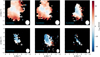 |
Fig. C.3 Radial velocity υrad maps for the mid-infrared transitions studied in this work. The grey star indicates the position of the protostar. The white circle indicates the PSF FWHM in the channel that contains the wavelength of the transition. Each coloured spaxel corresponds to a Gaussian fit with a peak height larger than 5σ, with σ indicating the uncertainty on the continuum flux as described in Appendix A. |
References
- Agra-Amboage, V., Cabrit, S., Dougados, C., et al. 2014, A&A, 564, A11 [NASA ADS] [CrossRef] [EDP Sciences] [Google Scholar]
- Anderson, J. M., Li, Z.-Y., Krasnopolsky, R., & Blandford, R. D. 2003, ApJ, 590, L107 [Google Scholar]
- Antoniucci, S., Nisini, B., Giannini, T., & Lorenzetti, D. 2008, A&A, 479, 503 [NASA ADS] [CrossRef] [EDP Sciences] [Google Scholar]
- Arce, H. G., Shepherd, D., Gueth, F., et al. 2007, in Protostars and Planets V, eds. B. Reipurth, D. Jewitt, & K. Keil, 245 [Google Scholar]
- Argyriou, I., Glasse, A., Law, D. R., et al. 2023, A&A, 675, A111 [NASA ADS] [CrossRef] [EDP Sciences] [Google Scholar]
- Arulanantham, N., McClure, M. K., Pontoppidan, K., et al. 2024, ApJ, 965, L13 [NASA ADS] [CrossRef] [Google Scholar]
- Bachiller, R. 1996, ARA&A, 34, 111 [NASA ADS] [CrossRef] [Google Scholar]
- Bai, X.-N., Ye, J., Goodman, J., & Yuan, F. 2016, ApJ, 818, 152 [Google Scholar]
- Bally, J. 2016, ARA&A, 54, 491 [Google Scholar]
- Benedettini, M., Giannini, T., Nisini, B., et al. 1999, ESA-SP, 427, 471 [NASA ADS] [Google Scholar]
- Bitner, M. A., Richter, M. J., Lacy, J. H., et al. 2008, ApJ, 688, 1326 [NASA ADS] [CrossRef] [Google Scholar]
- Black, J. H., & van Dishoeck, E. F. 1987, ApJ, 322, 412 [Google Scholar]
- Blandford, R. D., & Payne, D. 1982, MNRAS, 199, 883 [CrossRef] [Google Scholar]
- Böker, T., Arribas, S., Lützgendorf, N., et al. 2022, A&A, 661, A82 [NASA ADS] [CrossRef] [EDP Sciences] [Google Scholar]
- Böker, T., Beck, T. L., Birkmann, S. M., et al. 2023, PASP, 135, 038001 [CrossRef] [Google Scholar]
- Bron, E., Le Petit, F., & Le Bourlot, J. 2016, A&A, 588, A27 [NASA ADS] [CrossRef] [EDP Sciences] [Google Scholar]
- Burton, M. G., Hollenbach, D. J., & Tielens, A. G. G. 1992, ApJ, 399, 563 [NASA ADS] [CrossRef] [Google Scholar]
- Bushouse, H., Eisenhamer, J., Dencheva, N., et al. 2023, https://doi.org/10.5281/zenodo.7577320 [Google Scholar]
- Caratti o Garatti, A., Giannini, T., Nisini, B., & Lorenzetti, D. 2006, A&A, 449, 1077 [NASA ADS] [CrossRef] [EDP Sciences] [Google Scholar]
- Caratti o Garatti, A., Ray, T., Kavanagh, P., et al. 2024, A&A, 691, A134 [NASA ADS] [CrossRef] [EDP Sciences] [Google Scholar]
- Chapman, N. L., Mundy, L. G., Lai, S.-P., & Evans, N. J. 2008, ApJ, 690, 496 [Google Scholar]
- Chrysostomou, A., Bacciotti, F., Nisini, B., et al. 2008, A&A, 482, 575 [NASA ADS] [CrossRef] [EDP Sciences] [Google Scholar]
- Dabrowski, I. 1984, Can. J. Phys., 62, 1639 [NASA ADS] [CrossRef] [Google Scholar]
- Davis, C. J., Ray, T. P., Desroches, L., & Aspin, C. 2001, MNRAS, 326, 524 [Google Scholar]
- Davis, C. J., Stern, L., Ray, T. P., & Chrysostomou, A. 2002, A&A, 382, 1021 [NASA ADS] [CrossRef] [EDP Sciences] [Google Scholar]
- Davis, C. J., Cervantes, B., Nisini, B., et al. 2011, A&A, 528, A3 [NASA ADS] [CrossRef] [EDP Sciences] [Google Scholar]
- Delabrosse, V., Dougados, C., Cabrit, S., et al. 2024, A&A, 688, A173 [NASA ADS] [CrossRef] [EDP Sciences] [Google Scholar]
- D’Eugenio, F., Pérez-González, P. G., Maiolino, R., et al. 2024, Nat. Astron., 8, 1443 [CrossRef] [Google Scholar]
- Dionatos, O., Nisini, B., Cabrit, S., Kristensen, L., & Pineau Des Forêts, G. 2010, A&A, 521, A7 [NASA ADS] [CrossRef] [EDP Sciences] [Google Scholar]
- Dunham, M. M., Arce, H. G., Mardones, D., et al. 2014, ApJ, 783, 29 [NASA ADS] [CrossRef] [Google Scholar]
- Dutta, S., Lee, C.-F., Liu, T., et al. 2020, ApJS, 251, 20 [NASA ADS] [CrossRef] [Google Scholar]
- Dutta, S., Lee, C.-F., Johnstone, D., et al. 2022, ApJ, 925, 11 [NASA ADS] [CrossRef] [Google Scholar]
- Federman, S. A., Megeath, S. T., Rubinstein, A. E., et al. 2024, ApJ, 966, 41 [CrossRef] [Google Scholar]
- Ferreira, J., Dougados, C., & Cabrit, S. 2006, A&A, 453, 785 [NASA ADS] [CrossRef] [EDP Sciences] [Google Scholar]
- Flower, D., Des Forêts, G. P., & Walmsley, C. M. 2006, A&A, 449, 621 [NASA ADS] [CrossRef] [EDP Sciences] [Google Scholar]
- Frank, A., Ray, T. P., Cabrit, S., et al. 2014, in Protostars and Planets VI, eds. H. Beuther, R. S. Klessen, C. P. Dullemond, & T. Henning, 451 [Google Scholar]
- Fu, R. R., Weiss, B. P., Lima, E. A., et al. 2014, Science, 346, 1089 [Google Scholar]
- Fukutani, K., & Sugimoto, T. 2013, Prog. Surface. Sci., 88, 279 [Google Scholar]
- Furlan, E., Fischer, W. J., Ali, B., et al. 2016, ApJS, 224, 5 [Google Scholar]
- Gavilan, L., Vidali, G., Lemaire, J., et al. 2012, ApJ, 760, 35 [NASA ADS] [CrossRef] [Google Scholar]
- Giacalone, S., Teitler, S., Königl, A., Krijt, S., & Ciesla, F. J. 2019, ApJ, 882, 33 [NASA ADS] [CrossRef] [Google Scholar]
- Giannini, T., Nisini, B., Neufeld, D., et al. 2011, ApJ, 738, 80 [CrossRef] [Google Scholar]
- Gibb, A. G., & Heaton, B. D. 1993, A&A, 276, 511 [NASA ADS] [Google Scholar]
- Gieser, C., Beuther, H., Van Dishoeck, E., et al. 2023, A&A, 679, A108 [NASA ADS] [CrossRef] [EDP Sciences] [Google Scholar]
- Gordon, I. E., Rothman, L. S., Hargreaves, R. J., et al. 2022, J. Quant. Spec. Radiat. Transf., 277, 107949 [NASA ADS] [CrossRef] [Google Scholar]
- Harsono, D., Bjerkeli, P., Ramsey, J. P., et al. 2023, ApJ, 951, L32 [NASA ADS] [CrossRef] [Google Scholar]
- Hollenbach, D., Johnstone, D., Lizano, S., & Shu, F. 1994, ApJ, 428, 654 [NASA ADS] [CrossRef] [Google Scholar]
- Jacquemin-Ide, J., Ferreira, J., & Lesur, G. 2019, MNRAS, 490, 3112 [Google Scholar]
- Jakobsen, P., Ferruit, P., de Oliveira, C. A., et al. 2022, A&A, 661, A80 [NASA ADS] [CrossRef] [EDP Sciences] [Google Scholar]
- Jhan, K.-S., & Lee, C.-F. 2015, ApJ, 816, 32 [Google Scholar]
- Komaki, A., Nakatani, R., & Yoshida, N. 2021, ApJ, 910, 51 [NASA ADS] [CrossRef] [Google Scholar]
- Lahuis, F., van Dishoeck, E. F., Jørgensen, J. K., Blake, G. A., & Evans, N. J. 2010, A&A, 519, A3 [NASA ADS] [CrossRef] [EDP Sciences] [Google Scholar]
- Laraia, A. L., Gamache, R. R., Lamouroux, J., Gordon, I. E., & Rothman, L. S. 2011, Icarus, 215, 391 [NASA ADS] [CrossRef] [Google Scholar]
- Law, D. R., E. J. Morrison, Argyriou, I., et al. 2023, AJ, 166, 45 [NASA ADS] [CrossRef] [Google Scholar]
- Le Bourlot, J. 2000, A&A, 360, 656 [Google Scholar]
- Le Bourlot, J., Pineau des Forêts, G., & Flower, D. 1999, MNRAS, 305, 802 [NASA ADS] [CrossRef] [Google Scholar]
- Lee, C.-F. 2020, A&A Rev., 28, 1 [NASA ADS] [CrossRef] [Google Scholar]
- Lee, C.-F., Mundy, L. G., Reipurth, B., Ostriker, E. C., & Stone, J. M. 2000, ApJ, 542, 925 [NASA ADS] [CrossRef] [Google Scholar]
- Lee, C.-F., Li, Z.-Y., Shang, H., & Hirano, N. 2022, ApJ, 927, L27 [NASA ADS] [CrossRef] [Google Scholar]
- Li, Z.-Y., & Shu, F. H. 1996, ApJ, 472, 211 [NASA ADS] [CrossRef] [Google Scholar]
- Lique, F., Honvault, P., & Faure, A. 2014, Int. Rev. Phys. Chem., 33, 125 [CrossRef] [Google Scholar]
- Lodders, K. 2003, ApJ, 591, 1220 [Google Scholar]
- Maret, S., Bergin, E. A., Neufeld, D. A., et al. 2009, ApJ, 698, 1244 [NASA ADS] [CrossRef] [Google Scholar]
- Matt, S., & Pudritz, R. E. 2005, ApJ, 632, L135 [Google Scholar]
- McClure, M. 2009, ApJ, 693, L81 [NASA ADS] [CrossRef] [Google Scholar]
- Melnikov, S., Boley, P., Nikonova, N., et al. 2023a, A&A, 673, A156 [NASA ADS] [CrossRef] [EDP Sciences] [Google Scholar]
- Melnikov, S., Boley, P. A., Nikonova, N. S., et al. 2023b, A&A, 673, A156 [NASA ADS] [CrossRef] [EDP Sciences] [Google Scholar]
- Morisset, S., Aguillon, F., Sizun, M., & Sidis, V. 2005, J. Chem. Phys., 122, 194702 [NASA ADS] [CrossRef] [Google Scholar]
- Narang, M., Manoj, P., Tyagi, H., et al. 2024, ApJ, 962, L16 [NASA ADS] [CrossRef] [Google Scholar]
- Neufeld, D. A., Melnick, G. J., Sonnentrucker, P., et al. 2006, ApJ, 649, 816 [NASA ADS] [CrossRef] [Google Scholar]
- Neufeld, D. A., Nisini, B., Giannini, T., et al. 2009, ApJ, 706, 170 [NASA ADS] [CrossRef] [Google Scholar]
- Neufeld, D. A., DeWitt, C., Lesaffre, P., et al. 2019, ApJ, 878, L18 [NASA ADS] [CrossRef] [Google Scholar]
- Nisini, B., Giannini, T., Neufeld, D. A., et al. 2010, ApJ, 724, 69 [NASA ADS] [CrossRef] [Google Scholar]
- Nisini, B., Navarro, M. G., Giannini, T., et al. 2024, ApJ, 967, 168 [NASA ADS] [CrossRef] [Google Scholar]
- Pachucki, K., & Komasa, J. 2008, Phys. Rev. A, 77, 030501 [Google Scholar]
- Pagani, L., Vastel, C., Hugo, E., et al. 2009, A&A, 494, 623 [NASA ADS] [CrossRef] [EDP Sciences] [Google Scholar]
- Pascucci, I., Cabrit, S., Edwards, S., et al. 2023, in ASP Conf. Ser., 534, Protostars and Planets VII, eds. S. Inutsuka, Y. Aikawa, T. Muto, K. Tomida, & M. Tamura, 567 [Google Scholar]
- Pelletier, G., & Pudritz, R. E. 1992, ApJ, 394, 117 [NASA ADS] [CrossRef] [Google Scholar]
- Podio, L., Codella, C., Gueth, F., et al. 2016, A&A, 593, L4 [NASA ADS] [CrossRef] [EDP Sciences] [Google Scholar]
- Pontoppidan, K. M., Evans, N., Bergner, J., & Yang, Y.-L. 2024a, Res. Notes Am. Astron. Soc., 8, 68 [Google Scholar]
- Pontoppidan, K. M., Salyk, C., Banzatti, A., et al. 2024b, ApJ, 963, 158 [NASA ADS] [CrossRef] [Google Scholar]
- Rabenanahary, M., Cabrit, S., Meliani, Z., & Des Forêts, G. P. 2022, A&A, 664, A118 [NASA ADS] [CrossRef] [EDP Sciences] [Google Scholar]
- Ray, T. P., & Ferreira, J. 2021, New A Rev., 93, 101615 [NASA ADS] [CrossRef] [Google Scholar]
- Rigby, J., Perrin, M., McElwain, M., et al. 2023, PASP, 135, 048001 [NASA ADS] [CrossRef] [Google Scholar]
- Rohde, P., Walch, S., Seifried, D., et al. 2019, MNRAS, 483, 2563 [NASA ADS] [CrossRef] [Google Scholar]
- Ruffio, J.-B., Perrin, M. D., Hoch, K. K. W., et al. 2024, AJ, 168, 73 [NASA ADS] [CrossRef] [Google Scholar]
- Schofield, K. 1967, Planet. Space Sci., 15, 643 [Google Scholar]
- Schulz, W. R., & Le Roy, D. J. 1965, J. Chem. Phys., 42, 3869 [NASA ADS] [CrossRef] [Google Scholar]
- Schutzer, A. D. A., Rivera-Ortiz, P., Lefloch, B., et al. 2022, A&A, 662, A104 [NASA ADS] [CrossRef] [EDP Sciences] [Google Scholar]
- Sellek, A. D., Grassi, T., Picogna, G., et al. 2024, A&A, 690, A296 [NASA ADS] [CrossRef] [EDP Sciences] [Google Scholar]
- Shang, H., Krasnopolsky, R., Liu, C.-F., & Wang, L.-Y. 2020, ApJ, 905, 116 [NASA ADS] [CrossRef] [Google Scholar]
- Shinn, J.-H., Lee, H.-G., & Moon, D.-S. 2012, ApJ, 759, 34 [NASA ADS] [CrossRef] [Google Scholar]
- Shu, F., Najita, J., Ostriker, E., et al. 1994a, ApJ, 429, 781 [Google Scholar]
- Shu, F. H., Najita, J., Ruden, S. P., & Lizano, S. 1994b, ApJ, 429, 797 [Google Scholar]
- Sperling, T., Eislöffel, J., Fischer, C., et al. 2020, A&A, 642, A216 [CrossRef] [EDP Sciences] [Google Scholar]
- Sternberg, A., & Neufeld, D. A. 1999, ApJ, 516, 371 [NASA ADS] [CrossRef] [Google Scholar]
- Tabone, B., Raga, A., Cabrit, S., & Des Forêts, G. P. 2018, A&A, 614, A119 [CrossRef] [EDP Sciences] [Google Scholar]
- Tabone, B., Cabrit, S., Des Forêts, G. P., et al. 2020, A&A, 640, A82 [CrossRef] [EDP Sciences] [Google Scholar]
- Takahashi, J. 2001, ApJ, 561, 254 [NASA ADS] [CrossRef] [Google Scholar]
- Tielens, A. G. G. M., & Allamandola, L. J. 1987, in Interstellar Processes, 134, eds. D. J. Hollenbach, & H. A. Thronson, Jr., 397 [NASA ADS] [CrossRef] [Google Scholar]
- Timmermann, R. 1998, ApJ, 498, 246 [NASA ADS] [CrossRef] [Google Scholar]
- Tychoniec, Ł., van Gelder, M. L., van Dishoeck, E. F., et al. 2024, A&A, 687, A36 [NASA ADS] [CrossRef] [EDP Sciences] [Google Scholar]
- Wang, H., Weiss, B. P., Bai, X.-N., et al. 2017, Science, 355, 623 [NASA ADS] [CrossRef] [Google Scholar]
- Wilgenbus, D., Cabrit, S., Pineau des Forêts, G., & Flower, D. R. 2000, A&A, 356, 1010 [NASA ADS] [Google Scholar]
- Wright, G. S., Rieke, G. H., Glasse, A., et al. 2023, PASP, 135, 048003 [NASA ADS] [CrossRef] [Google Scholar]
- Yang, Y.-L., Green, J. D., Pontoppidan, K. M., et al. 2022, ApJ, 941, L13 [NASA ADS] [CrossRef] [Google Scholar]
- Yoshida, T., Hsieh, T.-H., Hirano, N., & Aso, Y. 2021, ApJ, 906, 112 [CrossRef] [Google Scholar]
- Zhang, Y., Arce, H. G., Mardones, D., et al. 2019, ApJ, 883, 1 [NASA ADS] [CrossRef] [Google Scholar]
- Zucker, C., Speagle, J. S., Schlafly, E. F., et al. 2019, ApJ, 879, 125 [NASA ADS] [CrossRef] [Google Scholar]
All Tables
Results of the rotation diagram fits to 1−0 S(0)–S(5) emission in three different apertures. The position of each aperture is indicated in Figure C.1. The distance (d) to the protostar in the image plane, ortho-to-para ratio (OPR), temperature (T) and column density (N) are listed for each aperture. The uncertainties are derived as described in Section 3.3.3.
All Figures
|
Fig. 1 MIRI MRS spectrum in an aperture extracted near knot A (see Figure C.2). The H2 0–0 S(1)–S(8) transition wavelengths are indicated with grey shading. The spectrum shows clear rotational H2 lines up to 0–0 S(7). |
| In the text | |
|
Fig. 2 NIRSpec spectrum extracted in an aperture 0′.′63 from the source, along the jet axis (see Figure C.1). The H2 1–0 S(0)–S(8) and 1–0 Q(7) transition wavelengths are indicated with grey shading. The 1–0 S(0)– S(5) and 1–0 Q(7) transitions are detected in this work. |
| In the text | |
|
Fig. 3 Molecular hydrogen 0–0 S(2) (left) and 1–0 S(1) (right) integrated flux maps of HOPS 315. The maps are derived from Gaussian fits to the emission lines in each spaxel. Black spaxels indicate spaxels where no line with a peak continuum-subtracted flux >5σ was detected (where σ is the continuum uncertainty) or that are out of the image field of view. White circles illustrate the size of the PSF FWHM at the transition wavelength. The dotted line indicates the jet axis, originating from the source (grey star). Two flux peaks can be identified in the left image, labelled with knot A and B. The former is also visible in the right image. Left: the white contours show the collimated 1–0 S(1) emission. The dashed-line parabola indicates the extent of the 2–1 12CO emission (230 GHz) observed by Dutta et al. (2022). Right: the NIRSpec PSF is surrounded by a yellow box such that it is easier to spot. |
| In the text | |
|
Fig. 4 Radial velocity υrad profile perpendicular to the jet axis for 00 S(1)–S(5). Positive values correspond to blueshift. Each datapoint is the median radial velocity along the spaxel column of the rotated image (see Section 3.2). The solid curves are second-order polynomial fits to the data. The curves are offset for clarity. The offset for each curve is annotated in the figure in the same colour. |
| In the text | |
|
Fig. 5 Corrected (1–0 S(1), top) and radial (0–0 S(1)–S(5), bottom) velocity profiles, respectively υcor and υrad . Positive velocity values correspond to blueshift. Each datapoint in the pure rotational molecular hydrogen curves is the median velocity along the spaxel column of the rotated image, while the 1–0 S(1) curve is derived from several apertures along the jet axis (see Section 3.2). The solid curves are exponential fits to the data. The rotational transition curves are offset for clarity. The offset for each curve is annotated in the figure in the same colour. |
| In the text | |
|
Fig. 6 0–0 S(l)–S(5) temperature map as derived from 0–0 S(l)–S(5) rotation diagrams. Left: the temperature map, with white contours derived from 0–0 S(2) emission outlining the positions of knot A and B. The white circle indicates the PSF FWHM that each transition integrated flux map has been smoothed to. Right: example of a single-spaxel rotation diagram. The measurements follow a straight line characterised by the temperature T and column density N as indicated in the grey box. |
| In the text | |
|
Fig. 7 Rotation diagrams for ro-vibrational H2 emission in three apertures at various distances (in the image plane) from the source. The ortho-to-para ratio (OPR) decreases further from the source. The temperature and column density corresponding to each fit are listed in Table 3. Plotted uncertainties do not include the extinction uncertainty, which affects each curve as illustrated in Figure 8. |
| In the text | |
|
Fig. 8 Rotation diagrams for ro-vibrational H2 emission in an aperture at 0′.′78 from the source (AP3), adopting three different values for the extinction AK . Fit parameter medians and uncertainties listed in the shaded box are derived using a sampling procedure (see Section 3.3.3). 100 sampled Boltzmann distribution fits are plotted for three different values of AK to portray its influence on the best-fit ortho-to-para ratio (OPR). |
| In the text | |
|
Fig. A.1 Example of a continuum fit and the estimation of its uncertainty for the near-infrared 1−0 S(4) line in AP2 (see Figure C.1). Top: The green lines indicate quadratic spline continuum fits through the sampled black anchor points. Only one in 30 sampled anchor points are shown for clarity. More opaque black or green colouring can be interpreted as a higher density of anchor points or continuum fits respectively. Bottom: The continuum-subtracted spectrum is plotted. The shaded area indicates the 1σ uncertainty of the continuum fits in each spectral bin. |
| In the text | |
|
Fig. B.1 Opening angle and width as function of deprojected distance z for four rotational H2 transitions. Top: flow FWHM as function of z for each transition. The straight line fits used to correct the opening angle formula (Equation B.1) are indicated with dashed lines. Bottom: outflow opening angles θFWHM spanned by the FWHM of the flow intensity profile as function of z for each transition. Straight line fits to the data for each transition are shown to guide the eye. |
| In the text | |
|
Fig. C.1 Continuum subtracted integrated flux map for the near-infrared transition 1−0 S(1). The grey star indicates the position of the protostar. The apertures used to construct rotation diagrams are indicated with green circles, where AP2 corresponds to the spectrum plotted in Figure 2. Each coloured spaxel corresponds to a Gaussian fit with a peak height larger than 5σ, with σ indicating the uncertainty on the continuum flux as described in Appendix A. The white circle in the bottom right indicates the PSF FWHM at the transition wavelength. |
| In the text | |
|
Fig. C.2 Continuum subtracted integrated flux maps for the mid-infrared transitions studied in this work. The grey star indicates the position of the protostar. The white circle indicates the PSF FWHM in the channel that contains the wavelength of the transition. The green circle in the 0–0 S(1) map indicates the aperture from which the spectrum shown in Figure 1 was extracted. Each coloured spaxel corresponds to a Gaussian fit with a peak height larger than 5σ, with σ indicating the uncertainty on the continuum flux as described in Appendix A. |
| In the text | |
|
Fig. C.3 Radial velocity υrad maps for the mid-infrared transitions studied in this work. The grey star indicates the position of the protostar. The white circle indicates the PSF FWHM in the channel that contains the wavelength of the transition. Each coloured spaxel corresponds to a Gaussian fit with a peak height larger than 5σ, with σ indicating the uncertainty on the continuum flux as described in Appendix A. |
| In the text | |
Current usage metrics show cumulative count of Article Views (full-text article views including HTML views, PDF and ePub downloads, according to the available data) and Abstracts Views on Vision4Press platform.
Data correspond to usage on the plateform after 2015. The current usage metrics is available 48-96 hours after online publication and is updated daily on week days.
Initial download of the metrics may take a while.