| Issue |
A&A
Volume 686, June 2024
|
|
|---|---|---|
| Article Number | A59 | |
| Number of page(s) | 29 | |
| Section | Interstellar and circumstellar matter | |
| DOI | https://doi.org/10.1051/0004-6361/202347832 | |
| Published online | 30 May 2024 | |
A deep search for large complex organic species toward IRAS16293-2422 B at 3 mm with ALMA
1
Leiden Observatory, Leiden University,
PO Box 9513,
2300 RA
Leiden,
The Netherlands
e-mail: nazari@strw.leidenuniv.nl
2
Department of Chemistry, Massachusetts Institute of Technology,
Cambridge,
MA
02139,
USA
3
Max-Planck-Institut für extraterrestrische Physik,
Giessenbachstr. 1,
85748
Garching,
Germany
4
Instituto de Astronomía, Universidad Nacional Autónoma de México, AP106,
Ensenada
CP 22830,
B.C.,
Mexico
5
Star and Planet Formation Laboratory, RIKEN Cluster for Pioneering Research, Wako,
Saitama
351-0198,
Japan
6
Niels Bohr Institute, University of Copenhagen,
Øster Voldgade 5–7,
1350
Copenhagen K.,
Denmark
7
SKA Organization, Jodrell Bank Observatory, Lower Withington,
Macclesfield, Cheshire
SK11 9FT,
UK
8
Laboratory for Astrophysics, Leiden Observatory, Leiden University,
PO Box 9513,
2300 RA
Leiden,
The Netherlands
9
Center for Space and Habitability, Universität Bern,
Gesellschaftsstrasse 6,
3012
Bern,
Switzerland
10
INAF – Osservatorio Astrofisico di Catania,
via Santa Sofia 78,
95123
Catania,
Italy
11
Departments of Astronomy and Chemistry, University of Virginia,
Charlottesville,
VA
22904,
USA
12
Center for Interstellar Catalysis, Department of Physics and Astronomy, Aarhus University,
Ny Munkegade 120,
Aarhus
C 8000,
Denmark
13
National Radio Astronomy Observatory,
Charlottesville,
VA
22903,
USA
14
Astrophysik/I. Physikalisches Institut, Universität zu Köln,
Zülpicher Str. 77,
50937
Köln,
Germany
15
Southwest Research Institute,
San Antonio,
TX
78238,
USA
Received:
30
August
2023
Accepted:
13
December
2023
Context. Complex organic molecules (COMs) have been detected ubiquitously in protostellar systems. However, at shorter wavelengths (~0.8 mm), it is generally more difficult to detect larger molecules than at longer wavelengths (~3 mm) because of the increase in millimeter dust opacity, line confusion, and unfavorable partition function.
Aims. We aim to search for large molecules (more than eight atoms) in the Atacama Large Millimeter/submillimeter Array (ALMA) Band 3 spectrum of IRAS 16293-2422 B. In particular, the goal is to quantify the usability of ALMA Band 3 for molecular line surveys in comparison to similar studies at shorter wavelengths.
Methods. We used deep ALMA Band 3 observations of IRAS 16293-2422 B to search for more than 70 molecules and identified as many lines as possible in the spectrum. The spectral settings were set to specifically target three-carbon species such as i- and n-propanol and glycerol, the next step after glycolaldehyde and ethylene glycol in the hydrogenation of CO. We then derived the column densities and excitation temperatures of the detected species and compared the ratios with respect to methanol between Band 3 (~3 mm) and Band 7 (~1 mm, Protostellar Interferometric Line Survey) observations of this source to examine the effect of the dust optical depth.
Results. We identified lines of 31 molecules including many oxygen-bearing COMs such as CH3OH, CH2OHCHO, CH3CH2OH, and c-C2H4O and a few nitrogen- and sulfur-bearing ones such as HOCH2CN and CH3SH. The largest detected molecules are gGg-(CH2OH)2 and CH3COCH3. We did not detect glycerol or i- and n-propanol, but we do provide upper limits for them which are in line with previous laboratory and observational studies. The line density in Band 3 is only ~2.5 times lower in frequency space than in Band 7. From the detected lines in Band 3 at a ≳ 6σ level, ~25–30% of them could not be identified indicating the need for more laboratory data of rotational spectra. We find similar column densities and column density ratios of COMs (within a factor ~2) between Band 3 and Band 7.
Conclusions. The effect of the dust optical depth for IRAS 16293-2422 B at an off-source location on column densities and column density ratios is minimal. Moreover, for warm protostars, long wavelength spectra (~3 mm) are not only crowded and complex, but they also take significantly longer integration times than shorter wavelength observations (~0.8 mm) to reach the same sensitivity limit. The 3 mm search has not yet resulted in the detection of larger and more complex molecules in warm sources. A full deep ALMA Band 2–3 (i.e., ~3–4 mm wavelengths) survey is needed to assess whether low frequency data have the potential to reveal more complex molecules in warm sources.
Key words: astrochemistry / stars: low-mass / stars: protostars / ISM: abundances / ISM: molecules
© The Authors 2024
 Open Access article, published by EDP Sciences, under the terms of the Creative Commons Attribution License (https://creativecommons.org/licenses/by/4.0), which permits unrestricted use, distribution, and reproduction in any medium, provided the original work is properly cited.
This article is published in open access under the Subscribe to Open model. Subscribe to A&A to support open access publication.
1 Introduction
In the interstellar medium (ISM) complex organic molecules (COMs), defined as species with at least six atoms containing carbon (Herbst & van Dishoeck 2009), are particularly prominent in the protostellar phase. Although other phases of star formation such as the prestellar phase (e.g., Bacmann et al. 2012; Jiménez-Serra et al. 2016; McGuire et al. 2020; Scibelli & Shirley 2020) and the later protoplanetary disk phase (Öberg et al. 2015; Walsh et al. 2016; Booth et al. 2021; Brunken et al. 2022) show detections of these species, COMs are more easily detectable in the line-rich protostellar envelopes due to their higher temperatures (e.g., Blake et al. 1987; Belloche et al. 2013; Bergner et al. 2017; van Gelder et al. 2020; Nazari et al. 2021; Yang et al. 2021; McGuire 2022; Bianchi et al. 2022; Hsu et al. 2022).
Many COMs, including species with more than eight atoms, are expected to form in ices under laboratory conditions (ethanol − CH3CH2OH, Öberg et al. 2009; Chuang et al. 2020; Fedoseev et al. 2022; aminomethanol − NH2CH2OH, Theulé et al. 2013; glycerol − HOCH2CH(OH)CH2OH, Fedoseev et al. 2017; 1-propanol − CH3CH2CH2OH, Qasim et al. 2019a,2019b; glycine − NH2CH2COOH, Ioppolo et al. 2021). However, there is a lot of debate regarding the ice or gas-phase formation of particular COMs (e.g., Ceccarelli et al. 2022). Two examples of these species are formamide (NH2CHO) and acetaldehyde (CH3CHO) for which both gas and ice formation pathways are suggested (e.g., Jones et al. 2011; Barone et al. 2015; Vazart et al. 2020; Chuang et al. 2020, 2021, 2022; Fedoseev et al. 2022; Garrod et al. 2022). To obtain clues as to the formation mechanism of COMs from an observational perspective, it is possible to search for the solid state signatures of COMs in ices (Schutte et al. 1999; Öberg et al. 2011) with telescopes such as the James Webb Space Telescope (Yang et al. 2022; McClure et al. 2023; Rocha et al., in prep.) using laboratory spectra available from, for example, the Leiden Ice Database for Astrochemistry (Rocha et al. 2022) and to examine the gas-phase correlations between different COMs in large samples of sources (Belloche et al. 2020; Coletta et al. 2020; Jørgensen et al. 2020; Nazari et al. 2022a; Taniguchi et al. 2023; Chen et al. 2023). However, observations and models show that physical effects such as the source structure or dust optical depth could affect the snowline locations, gas-phase emission, and column density correlations of simple and complex molecules (Jørgensen et al. 2002; Persson et al. 2016; De Simone et al. 2020; Nazari et al. 2022b, 2023a,b; Murillo et al. 2022a). Hence, interpretations of COM formation routes based on gas-phase observations can be affected by these physical factors. For example, an anticorrelation between column densities of two species (or a large scatter in the column density ratios) could have a physical origin rather than a chemical origin.
Among the low-mass protostars, the IRAS16293-2422 (IRAS16293 hereafter) triple protostellar system (Wootten 1989; Maureira et al. 2020) is one of the closest protostars, and one of the richest and most well-studied objects from a chemical perspective. The first detection of methanol (CH3OH; the simplest COM) toward a low-mass protostar was carried out by van Dishoeck et al. (1995) for this system. Since then, its chemistry and in particular the COMs in this system have been studied in more detail (Cazaux et al. 2003; Butner et al. 2007; Bisschop et al. 2008; Ceccarelli et al. 2010; Jørgensen et al. 2011, 2012; Kahane et al. 2013; Jaber et al. 2014). More recently, the Protostellar Interferometric Line Survey (PILS; Jørgensen et al. 2016) studied IRAS16293 in Band 7 (~329.147 − 362.896 GHz) of the Atacama Large Millimeter/submillimeter Array (ALMA). This survey detected many COMs for the first time in the ISM, adding further information on complexity in space (Coutens et al. 2016, 2022; Lykke et al. 2017; Calcutt et al. 2018a; Jørgensen et al. 2018; Manigand et al. 2019, 2021).
However, a limitation of higher-frequency observations of ALMA (~330 GHz) is the higher degree of line blending. The reason is that for observations probing the same gas, the line width – although constant in velocity space – increases in frequency space (Jørgensen et al. 2020). Therefore, the detection of larger COMs with more than eight atoms, which have relatively weak lines, is expected to be easier at lower frequencies. Moreover, the heavier molecules have their Boltzmann distribution peak at lower frequencies than the lighter molecules at the same excitation temperature, and thus their lines are stronger at lower frequencies and they are more easily detected at long wavelength observations. On the other hand, the Boltzmann peak moves to the higher frequencies for higher temperatures (see Fig. 2 of Herbst & van Dishoeck 2009). Therefore, if the large molecules are thermally sublimated in the inner hot regions around the protostar (tracing warm or hot regions), it is difficult to observe these larger species even at low frequencies (although favored), unless the data are sensitive enough, which can be achieved at the expense of the angular resolution and longer integration times. The combination of the increase in line width in frequency space and the Boltzmann distribution peak of the lighter molecules being at higher frequencies also lead to spectra being more crowded, and thus it is more difficult to detect large molecules at high frequencies.
Moreover, dust optical depth effects could be an important issue at higher-frequency ALMA Bands 6 (~240 GHz) and 7 (~330 GHz). This is because of the larger dust opacity of ~ 1 mm-sized grains at shorter wavelengths (i.e, higher frequencies). For example, López-Sepulcre et al. (2017) found that NGC 1333 IRAS 4A1 in Perseus does not host any COMs when searched for with ALMA and the Plateau de Bure Interferometer. However, later, De Simone et al. (2020) detected methanol around this source at longer wavelengths with the Very Large Array (VLA). Another example is the ring-shaped structure of methanol around the dust continuum in the massive protostellar system 693050 (also known as G301.1364-00.2249) observed by van Gelder et al. (2022b) at ~220 GHz with ALMA, which indicates dust attenuation on-source.
For this work, we used the deep Band 3 ALMA observations of IRAS16293 B to search for larger species (more than eight atoms). This dataset was specifically optimized to hunt for molecules such as glycerol and i- and n-propanol. Although the main aim is to specifically hunt for large molecules, we identified as many molecules as possible from the Cologne Database for Molecular Spectroscopy (CDMS; Müller et al. 2001, 2005) and the Jet Propulsion Laboratory database (JPL; Pickett et al. 1998) in our data. We fit the spectrum to derive the column densities and excitation temperatures of the detected species and we compared our results with those of PILS in Band 7. In particular, we examined whether dust attenuation is important for column densities and their ratios with respect to methanol (typically used as a reference species).
The paper is structured such that the observations are explained in Sect. 2. The results including the detected species and their column densities and excitation temperatures are given in Sect. 3. We discuss our findings, in particular the comparison with the PILS results in Sect. 4. Finally, we present our conclusions in Sect. 5.
2 Observations and methods
2.1 Data
This paper uses the data of IRAS16293 B taken with ALMA in Band 3 (project code: 2017.1.00518.S; PI: E. F. van Dishoeck). For more information on the data calibration, reduction, and imaging, as well as the first results on the gas accretion flow in the IRAS16293 system, readers can refer to Murillo et al. (2022b); here we give a brief description of the data. We used the data with the configuration C43-4, which were calibrated with the CASA pipeline (McMullin et al. 2007) and then self-calibrated with CASA. Continuum subtraction was done on the self-calibrated image datacubes using STATCONT (Sánchez-Monge et al. 2018).
The data have an angular resolution of ~0.9″ × 0.7″, which is larger than that of PILS (~0.5″). The frequency ranges covered were ~90.59–91.41 GHz (continuum), ~93.14–93.20 GHz, and ~103.28–103.52 GHz. After conversion of the flux to brightness temperature, the rms found from line-free regions in each spectral window was ~0.1 K, ~0.3 K, and 0.2 K (comparable to PILS), respectively, following a 171.7 minute on-source integration time. The spectral resolution was 0.805 km s−1, 0.049 km s−1, and 0.088 km s−1. Given that the lines have a full width at half maximum (FWHM) of ~1–2 km s−1, some lines are not fully resolved in the continuum window. The frequency range was optimized to cover transitions of larger species such as glycerol as well as i- and n-propanol. It also serendipitously covered transitions from other oxygen- and nitrogen-bearing COMs including glycolaldehyde (CH2OHCHO), propanal (g-C2H5CHO), and glycolonitrile (HOCH2CN). The spectrum of IRAS16293 B (Fig. 1) was extracted from the same 0.5″ offset position from the continuum peak of B that was used in many of the works from ALMA-PILS (αJ2000 = 16h32m22s.58 and δJ2000 = −24°28′32.8″, Coutens et al. 2016; Jørgensen et al. 2018; Calcutt et al. 2018b). Maps of a few common species tracing cold gas structures are presented in Murillo et al. (2022b).
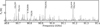 |
Fig. 1 Spectrum of IRAS16293 B Band 3 data for the continuum window. A few strong lines are highlighted; for the full line identification and fitting, readers can refer to Fig. B.1. We note that “X” indicates a line that has not been identified yet and that was not (fully) fitted with the considered molecules for this work. The spectrum of IRAS16293 B is line rich even at ALMA Band 3 wavelengths (~3 mm). |
2.2 Spectral modeling
For this work, we identified as many molecules as possible using the CASSIS1 spectral analysis tool (Vastel et al. 2015). We consider a molecule as detected if it has at least three lines at a peak of the ≥3σ level. We also report column densities of the molecules that have one or two detected lines without any overprediction of the emission in the spectrum. These column densities are only tentative and not as robust as those found for molecules with many detected lines because of the limited frequency coverage, but they should be reliable for the most abundant and common molecules such as 13CH3OH. Using CASSIS, we fit for the identified molecules. In the fitting procedure, the spectrum was considered as a whole; and all the lines of a molecule were fitted simultaneously assuming local thermodynamic equilibrium (LTE) conditions. The fitting followed a similar procedure as the fit-by-eye method used in Nazari et al. (2022a). This includes varying the column densities (N) and excitation temperatures (Tex) in the LTE models to produce a synthetic spectrum that matches the data (for more information on this process, see below). The line lists were taken from the CDMS (Müller et al. 2001, 2005) or the JPL database (Pickett et al. 1998). Appendix A gives more information on the spectroscopic studies used for our assignments and Table B.2 presents the transitions covered in the data.
In the fitting process, the FWHM was first fitted for the unblended line(s) of each molecule. Then it was fixed to that value when the column density and excitation temperature were being determined. The FWHM for all considered species is ~1.8 ± 0.5 km s−1, except for (formic acid) t-HCOOH, which is slightly lower (i.e., ~1 km s−1). The typical FWHM here is ~1.5–2 times larger than the typical FWHM found in PILS (~1 km s−1). However, the spectral resolution for the continuum spectral window (i.e., the major spectral window where most lines lie; Fig. B.1) is ~0.8 km s−1 in this work. This implies that not all lines are spectrally resolved. Therefore, the higher FWHM measured here could be due to this low spectral resolution. The excitation temperature was only fitted if there were enough (≥2) detected lines of a molecule with a range of Eup (e.g., ~100–400 K). The typical uncertainty on the excitation temperature is ~ ± 50 K. If not enough lines with a range of Eup were detected, the temperature is fixed to 100 K, which is similar to excitation temperatures assumed or found for many species in PILS (Lykke et al. 2017; Calcutt et al. 2018b; Jørgensen et al. 2018). The exceptions to this rule were t-HCOOH and NH2CHO. Only one line was detected for each of these two molecules and their temperatures were fixed to 300 K to be consistent with PILS (Coutens et al. 2016; Jørgensen et al. 2018). Moreover, for the isotopologues for which a determination of the excitation temperature was not possible, the temperature was fixed to that of the other isotopologues with a determined Tex. Deuterated methanol, CH2DOH, has three detected lines, with upper energy levels of ~10 K, ~100 K, and ~400 K. It was not possible to fit all three lines of this molecule with a single excitation temperature. Therefore, we adopted the same temperature as the methanol isotopologue that has the most lines detected (i.e., CHD2OH). However, this temperature fits the ~100 K line better than the other two. For aGg′-(CH2OH)2, we note that again a single temperature cannot fit all of its lines. In particular, the line at 90.593 GHz with Eup = 19 K gets overestimated regardless of the temperature assumed. This could be because of this line being (marginally) optically thick; therefore, we ignored this line and fixed the temperature to that of gGg′-(CH2OH)2. A similar two-component temperature structure was found for glycolonitrile (HOCH2CN) toward IRAS 16293 B (Zeng et al. 2019). Using this method the rest of the lines are explained reasonably well (i.e., within ~20–30%; see Fig. B.1).
The column density was always treated as a free parameter. The uncertainty on column densities was measured from the same method explained in Nazari et al. (2022a) and the typical uncertainty from the fits is on the order of 20%. Figure B.1 shows the final fitted model for each molecule. As this figure shows, there are still unidentified lines in the spectrum (see Sect. 3.1 for more details). In this process, the source velocity was fixed to Vlsr = 2.7 km s−1 and a beam dilution of unity was assumed resulting in our column densities being representative of those within a beam. This is different from the assumption in PILS where the source size was set to 0.5″. Nevertheless, this assumption does not change the conclusions as long as the lines are optically thin. This is because only the number of molecules and their ratios are of interest here. The number of molecules (![$\[\boldsymbol{\mathcal{N}}\]$](/articles/aa/full_html/2024/06/aa47832-23/aa47832-23-eq1.png) ) is constant regardless of the source size assumed. The number of molecules is equal to N × A, where A is the emitting area. Hence a decrease in the emitting area increases the fitted column densities and vice versa such that the number of molecules stays the same as long as the lines stay optically thin (also see van Gelder et al. 2022a; Nazari et al. 2023c). However, we note that with this assumption, we ignored any potential differences between the emitting areas of various molecules. This assumption can only be improved with higher angular resolution data than presented in this work.
) is constant regardless of the source size assumed. The number of molecules is equal to N × A, where A is the emitting area. Hence a decrease in the emitting area increases the fitted column densities and vice versa such that the number of molecules stays the same as long as the lines stay optically thin (also see van Gelder et al. 2022a; Nazari et al. 2023c). However, we note that with this assumption, we ignored any potential differences between the emitting areas of various molecules. This assumption can only be improved with higher angular resolution data than presented in this work.
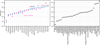 |
Fig. 2 Column density ratios of detected species and upper limits with respect to methanol. Left: column density ratios for the detected species with respect to methanol for our Band 3 data (blue). The same ratios from PILS in Band 7 (pink) are also shown for comparison (see the text for references). The hollow symbols show the species that only have one detected line. Right: ratios of the upper limits measured in this work (Table B.1) with respect to methanol. In both panels, the species are ordered from left to right by increasing Band 3 ratios with respect to methanol. |
3 Results
3.1 Deep search and the considered species
The spectrum of IRAS16293 B at ~3 mm wavelengths is line rich and crowded (see Fig. 1 for an overview). In total, 16 molecules were detected and 15 were tentatively detected (see Table 1). Ratios of the detected molecules with respect to methanol are presented in the left panel of Fig. 2 (see Sect. 4.2.3 for a discussion on the comparison with PILS). Among these species, many “standard” COMs such as methanol (CH3OH), ethanol (CH3CH2OH), ethyl cyanide (CH3CH2CN), acetaldehyde (CH3CHO), methyl formate (CH3OCHO), and dimethyl ether (CH3OCH3) with some of their isotopologues are apparent. The frequency range did not cover transitions of CH3CN and HNCO or their isotopologues. We also detected one carbon chain molecule, cyanoacetylene (HCCCN). It should be noted that the frequency range of the observations covers HC5N transitions, but this carbon chain was not detected toward IRAS16293 B. It was, however, detected ~12″ off-source to the west of IRAS16293 B (Murillo et al. 2022b).
This dataset was specifically taken to search for large species due to the expected lower line density and line confusion in Band 3 in comparison with Band 7 used for PILS. Moreover, at the same excitation temperature, heavier molecules have their Boltzmann distribution peak at lower frequencies, which increases the chance of detecting them in Band 3. Particularly, the frequency windows were selected to search for glycerol (HOCH2CH(OH)CH2OH) and propanol (C3H7OH). Isopropanol (i-C3H7OH) and normal-propanol (n-C3H7OH) have been detected previously in the ISM (Belloche et al. 2022; Jiménez-Serra et al. 2022), although not yet in IRAS16293 B (Taquet et al. 2018). In addition to these molecules, we searched for and detected large and complex species such as aGg’- and gGg’-ethylene glycol (CH2OH)2, glycolaldehyde (CH2OHCHO), and acetone (CH3COCH3).
Table B.1 presents the upper limits of the molecules we searched for but do not detect, including glycerol and isopropanol. The largest molecule that we searched for is cyanonaphthalene (C10H7CN; McNaughton et al. 2018) and its upper limit is given in Table B.1. Figures 3, B.2, and B.3 present the lines of g-Isopropanol, Ga-n-propanol, and G′Gg′gg′-Glycerol with the model upper limits. We note that in Fig. 3, the lines that seem to agree well with the data in the first two panels are well explained with other molecules (see the cyan line as the total fitted model for the detected or tentatively detected species), and thus they could not be the lines of g-Isopropanol. Moreover, the line at around 91.345 GHz overestimates the data. The ratio of measured upper limits with respect to methanol are presented in the right panel of Fig. 2. The ratios span a range of ~5 orders of magnitude from ~10−6 to ~0.1, which is similar to the range seen for the detected molecules (left panel of Fig. 2).
The line density of the lines detected at ≳6σ level in Band 3 (~100 GHz) data is one per ~8.5 MHz (see Fig. B.1 for the variations in line density across the frequency range), while the line density is one per ~3.5 MHz in Band 7 (~345 GHz; Jørgensen et al. 2016). Therefore, as expected, the spectrum has a lower line density in Band 3 than Band 7, although only by a factor of ~2.5, resulting in a relatively line-rich spectrum still. Although many lines (~70%) in the Band 3 spectrum of IRAS16293 B were identified, we could not associate any simple or complex species to ~25–30% of lines at the ≳6σ level. Potentially more high-resolution laboratory spectra are needed to identify those lines. This is particularly important for the (doubly) deuterated isotopologues of known COMs and larger COMs with more than eight atoms.
3.2 Fitting results for the detected species
Derived column densities and excitation temperatures are given in Table 1. The measured excitation temperatures span a range between ~50 and ~300 K. Figure B.4 presents the excitation temperatures where a determination was possible for molecules with sufficient detected lines. The species on the x-axis are roughly ordered by increasing binding energies in the ice from left to right (Minissale et al. 2022; Ligterink & Minissale 2023). The error bars are too large to robustly confirm whether there is any correlation between the excitation temperature and binding energy.
The column densities measured here span a range of ~4 orders of magnitude. The most abundant molecule is methanol, after that (and its isotopologues), CH3OCHO and CH3OCH3 were found to be the second and third most abundant species as found in many other protostellar systems (Coletta et al. 2020; Chen et al. 2023). The column density of CH3OH was determined by scaling the 13CH3OH column density by 12C/13C of 68 (Milam et al. 2005) and was found to be 8.2 × 1018 cm−2 in the ~1″ beam. We note that the 13CH3OH lines used for measurement of column density of this molecule are relatively weak and hence optically thin. They either have a large Eup(~500 K) or a low Aij (~6 × 10⁻⁸ s−1). Therefore, 13CH3OH in this study should robustly determine the column density of the major isotopologue without the need for CH318OH. The least abundant molecule at the 0.5″ offset location is HCCCN with a column density of 6.2 × 1013 cm−2 (see Murillo et al. 2022b for its map).
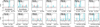 |
Fig. 3 Lines of g-Isopropanol and the model for its upper limit in red dashed lines (1.5 × 1016 cm−2). Gray is the data and cyan is the total fitted model from the detected and tentatively detected species. The vertical dotted lines show the transition frequency of each line. The Eup and Aij are printed in the top left of each panel. The line that was used to find the 3σ upper limit is indicated by an “X” in the top right. The horizontal dashed lines show the 3σ level. Only lines with Aij > 10−6 s−1 and Eup < 300 K are shown. |
3.3 Glycolonitrile and ethylene oxide
Here we focus on the tentative detection of HOCH2CN (glycolonitrile) and c-C2H4O (ethylene oxide). These two molecules are among the less common species studied toward protostars in Table 1. Glycolonitrile is an interesting interstellar molecule to study given that it is a rarely observed prebiotic molecule. Ethylene oxide is an interesting molecule because it is the only species in Table 1 with a cyclic structure.
Glycolonitrile was detected toward IRAS 16293 B using lower frequency (≲266 GHz) observations than PILS (Zeng et al. 2019). Later it was also detected in PILS by Ligterink et al. (2021), mainly toward the half-beam offset position (~0.25″ offset from the continuum peak) and not the full-beam offset position (0.5″ offset). It is interesting that in the Band 3 data, HOCH2CN was tentatively detected toward the full-beam offset position of PILS. This could be due to the larger beam size of the Band 3 observations and the inclusion of the hotter gas close to the protostar in the beam given that the binding energy of this molecule is relatively high (~10400 K; Ligterink & Minissale 2023).
Our tentative column density ratio of HOCH2CN/CH3OH (~10−4) agrees well with what Ligterink et al. (2021) found for this source in Band 7. Moreover, our column density for HOCH2CN, after correction for beam dilution (see Sect. 4.2.2), is within a factor of about two of what Zeng et al. (2019) found for their warm component of the same source from their Band 3 data. Moreover, glycolonitrile has been (tentatively) detected toward other objects such as the Serpens SMM1-a protostar and the G+0.693–0.027 molecular cloud with similar HOCH2CN/CH3OH ratios of a few 10−4 (Requena-Torres et al. 2006; Ligterink et al. 2021; Rivilla et al. 2022). A recent study searched for its minor isotopologues in IRAS 16293B and SMM1-a, but it resulted in non-detections (Margulès et al. 2023).
Ethylene oxide has been detected toward several objects, mainly high-mass protostars, but also pre-stellar cores and the comet 67P (Dickens et al. 1997; Nummelin et al. 1998; Ikeda et al. 2001; Requena-Torres et al. 2008; Bacmann et al. 2019; Drozdovskaya et al. 2019). This molecule has also been detected toward IRAS 16293 A and B by PILS (Lykke et al. 2017; Manigand et al. 2020). The ratio for ethylene oxide to methanol from this work is ~7 × 10⁻⁴, which agrees well with the ratio from PILS of ~3–6 × 10⁻⁴ (Lykke et al. 2017; Jørgensen et al. 2016, 2018). Its deuterated species were studied and detected toward IRAS 16293 B by Müller et al. (2023a,b). We also tentatively detected one of its deuterated species, c-C2H3DO, in our Band 3 data. The ratio of this molecule with respect to methanol in our data is ~1–2 × 10⁻⁴ which agrees well with the same ratio in PILS (~9 × 10⁻⁵; Jørgensen et al. 2018; Müller et al. 2023a).
4 Discussion
4.1 Dust optical depth
For this section we calculated the continuum optical depth at ~348.815 GHz (corresponding to ALMA Band 7) and at ~91 GHz (corresponding to ALMA Band 3). The continuum optical depth as a zeroth-order approximation is given by (see Rivilla et al. 2017 and van Gelder et al. 2022b)
![$\[\tau_v=-\ln \left(1-\frac{F_v}{\Omega_{\text {beam }} B_v\left(T_{\text {dust }}\right)}\right),\]$](/articles/aa/full_html/2024/06/aa47832-23/aa47832-23-eq2.png) (1)
(1)
where Fν is the continuum flux density within the beam, Ωbeam = πθminθmaj/(4 ln(2)) is the beam solid angle with θmin and θmaj as the beam minor and major axes, Bν is the Planck function, and Tdust is the dust temperature. We took the continuum image of the PILS survey at ν~348.815 GHz from the ALMA archive and found Fν to be within the beam of those observations at the peak of the continuum and at the ~0.5″ offset position where the spectrum was extracted. For this measurement we used CASA (McMullin et al. 2007) version 6.5.2.26 and found the continuum flux density to be ~1.16 Jy beam−1 and ~0.55 Jy beam−1 at the peak and the offset position. We did the same for the Band 3 data at a frequency of ~91 GHz and found the Band 3 continuum flux density to be ~9.07 × 10⁻² Jy beam−1 and ~5.25 × 10⁻² Jy beam−1 at the peak and the offset positions, respectively. Next, we calculated τdust for a range of dust temperatures that are feasible for IRAS 16293B as suggested by Jacobsen et al. (2018).
Figure 4 presents the continuum optical depth for the various temperatures. The temperature of the inner regions based on models of Jacobsen et al. (2018) is ~90 K. At 90 K, both the PILS and Band 3 peak continuum are marginally optically thick with the PILS continuum having an optical depth of ~1.5 times larger. However, at the location off-source, the dust optical depth for the PILS continuum is almost the same as that of Band 3, which is ~0.15. Therefore, it is safe to assume that the dust at the offset location at Tdust = 90 K is almost completely optically thin in Band 3 and Band 7 datasets. Even assuming the unrealistic worst case scenario of Tdust = 30 K in Fig. 4 and assuming that all the dust is in a column between the observer and the protostar, the difference between Band 3 and Band 7 dust attenuation (i.e., e−τ) is around 25% at the offset location at most.
Fitted parameters for detected and tentatively detected Band 3 species toward IRAS 16293 B.
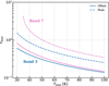 |
Fig. 4 Continuum optical depth as a function of temperature at the peak of the continuum (dashed) and the 0.5″ offset position where the spectrum was extracted (solid line). Blue shows the optical depth for the Band 3 continuum at a frequency of ~91 GHz and pink shows the PILS continuum at a frequency of ~348.815 GHz. |
4.2 Comparison with PILS
In this section we compare the excitation temperatures and column densities of the same molecules detected in the PILS Band 7 survey and this work.
4.2.1 Excitation temperature
The measured excitation temperatures are presented in Fig. B.4. The species are roughly ordered by increasing binding energy (a measure of how strongly bound a molecule is in ices) from left to right. However, given that the uncertainties are relatively large, the number of detected lines for each species is small, and the lines are biased toward lower Eup; it is not possible to identify a clear trend between the binding energies (or sublimation temperatures) and excitation temperatures. Another effect that can complicate the picture and change Fig. B.4 is that the molecules with lower binding energies than water are expected to desorb with water if initially mixed with it (Collings et al. 2004; Busch et al. 2022; Garrod et al. 2022). This would be in line with the measured excitation temperatures of the molecules toward the left hand side of Fig. B.4 being at around ~100 K (i.e., the desorption temperature of water). Therefore, a strong trend might not be expected in Fig. B.4.
Nevertheless, our excitation temperatures mostly agree with those found by Jørgensen et al. (2018) for IRAS 16293 B. The only exceptions are CH3OCHO and CH3CH2OH where their excitation temperatures are found to be higher in PILS. This could be due to the lines that are covered in the Band 3 data having a lower Eup than those covered in the Band 7 data. For example, if the two lines of CH3CH2OH with Eup~80–90 K are ignored, a fit at Tex~240 K (i.e., agreeing with the PILS temperature) can match the brightness temperatures of the rest of the lines within ~40–50%. Our excitation temperatures also agree well with what is found for the companion source, IRAS 16293A, in PILS (Manigand et al. 2020).
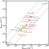 |
Fig. 5 Column density of the various molecules from the ALMA Band 7 observations (PILS; ~345 GHz) as a function of those from Band 3 (~100 GHz). Beam dilution was corrected for the column densities in this figure. Dashed lines present where the values of the y-axis are the same as the values of the x-axis, where they are ten times higher and ten times lower than the values of the x-axis. |
4.2.2 Column density
Making a direct comparison of the column densities from PILS and this work should be done with caution due to the different beam sizes in the two sets of observations. Therefore, before comparison, column densities of Band 7 were corrected to match the Band 3 results. PILS studies use a source size of 0.5″ in their analysis, while we found the column densities averaged over the Band 3 beam. Our assumption corresponds to the Band 3 emission filling the beam uniformly (i.e., θs ≫ θb). The PILS column densities were converted to an average over the PILS beam (or filling the PILS beam uniformly) by multiplication with their beam dilution factor of ![$\[\\frac{0.5^2}{0.5^2+0.5^2}\]$](/articles/aa/full_html/2024/06/aa47832-23/aa47832-23-eq73.png) = 0.5. After this modification, we also investigated how the different beam sizes in PILS and our study can affect the comparison (assuming that the column densities are averaged over the respective beams). Figure B.5 presents a two-dimensional Gaussian distribution with two circular regions representing the beams of Band 3 and Band 7. Assuming a uniform beam, we calculated the mean in the two beams and found around a 10% difference between these two, which is smaller than the typical uncertainties on the column densities and it was thus ignored.
= 0.5. After this modification, we also investigated how the different beam sizes in PILS and our study can affect the comparison (assuming that the column densities are averaged over the respective beams). Figure B.5 presents a two-dimensional Gaussian distribution with two circular regions representing the beams of Band 3 and Band 7. Assuming a uniform beam, we calculated the mean in the two beams and found around a 10% difference between these two, which is smaller than the typical uncertainties on the column densities and it was thus ignored.
Figure 5 presents the column densities from PILS and this work after correction for beam dilution. The column densities of PILS are taken from Coutens et al. (2016; NH2CHO), Jørgensen et al. (2016; CH2OHCHO, CHDO-HCHO, gGg-(CH2OH)2, and CH3COOH), Calcutt et al. (2018b; CH3CH2CN, HC3N), Jørgensen et al. (2018; CH3OH, 13CH3CHO, CH3CDO, CH3CHO, CH2DOH, CH3CH2OH, a-CH3CHDOH, CH3OCH3, CH3OCHO, a-a-CH2DCH2OH, and t-HCOOH), Persson et al. (2018; D2CO), Manigand et al. (2020; CH2DCHO), Drozdovskaya et al. (2022; CHD2OH), Ilyushin et al. (2022; CD3OH), Drozdovskaya et al. (2018; CH3SH), Ferrer Asensio et al. (2023; CHD2CHO), and Lykke et al. (2017; CH3COCH3). In addition, we did not include 13CH2OHCHO and gGg-(CH2OH)2 in Fig. 5 because our measured column densities are approximate. Moreover, the column density of CH3COOH in PILS was found from old spectroscopic data (Jørgensen et al. 2016). To avoid a bias, we redid the fit to CH3COOH in the Band 7 data using new spectroscopic data (Ilyushin et al. 2013; see Appendix A), and found that the column density in Jørgensen et al. (2016) was underestimated by a factor of about two. Therefore, in this work we refer to the updated column density of CH3COOH using the new spectroscopic data (~1.2 × 10¹⁶).
Figure 5 shows that the column densities from the Band 3 observations generally agree with those of PILS. There are a few data points where the Band 3 column densities are ≳3 times higher than those of Band 7. Among those molecules, NH2CHO and CH3CH2CN seem to be outliers that have Band 3 column densities that are ten times higher than Band 7. However, because the column densities of these two molecules in this work were measured based on only one line, those values should be considered with caution. Therefore, we excluded these two molecules from further analysis.
Taking only the molecules with at least three detected lines in Band 3 (see Table 1), the average of (log10 of) the Band 3 column densities weighted by the uncertainty on each data point is 4.4 × 1016 cm−2. This value for Band 7 column densities (measured using many more lines per molecule due to the larger frequency coverage) is 2.7 × 1016 cm−2. These two agree well within the uncertainties. Moreover, the scatter around the line of NBand3 = NBand7 is a factor of 1.9 below the line and 1.8 above the line. Therefore, it can be concluded that there is a tight, one-to-one correlation between the two column densities with a scatter of less than a factor of two. This agrees well with the low dust optical depth found for the Band 3 and Band 7 observations at the offset location where the spectra were extracted.
4.2.3 Ratios
The column density ratios are normally more informative than absolute column densities because the latter depends on the beam and the assumed beam dilution factor. The left panel of Fig. 2 shows that the ratios with respect to methanol from Band 3 agree well with those from Band 7 (PILS) for almost all molecules. Figure 6 presents the ratio between the Band 3 and Band 7 results for individual molecules. This figure shows, even more clearly, that the results from the Band 3 data (this work) generally agree within a factor of about two with the results from the Band 7 data. Four molecules show larger than a factor of two difference between the two datasets and they are marked with an ellipse. This could be due to the lines of these species becoming optically thick. This argument is more convincing for CH3CHO and CH3CH2OH given that there is good agreement between Band 3 and Band 7 results for their minor isotopologues. Moreover, the value for CH2DOH is likely uncertain given that no single temperature could be fitted to its lines and hence the assumed Tex does not fit all its lines equally well in this work (see Sect. 2.2). The slight variations between the Band 3 and Band 7 ratios could be due to the smaller number of lines covered in the Band 3 dataset compared with the PILS dataset, which also sets looser constraints on the excitation temperatures. Another factor in these variations could be the different beam sizes in the two datasets (see Sect. 4.2.2).
We found a good match between Band 3 and Band 7 data when comparing the ratios of the various COMs relative to methanol. The molecules that have column densities with a factor of >2 difference between Band 3 and Band 7 in Fig. 5 (i.e., t-HCOOH, CD3OH, and CHD2CHO) show good agreement (factor of <2) when their column density ratios with respect to methanol are compared between the two sets of observations.
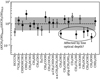 |
Fig. 6 Ratio between Band 3 and PILS column density ratios with respect to methanol (i.e., the ratio of blue to pink from the left panel of Fig. 2). The horizontal dashed line indicates where the ratio between Band 3 and PILS are the same. The shaded gray area indicates the region with a factor of two difference between Band 3 and PILS results. The species are ordered in the same way as in the left panel of Fig. 2. The hollow symbols show the species that have only one detected line. |
4.3 Comparison with other studies
In this section we put some of the measured ratios (Fig. 2) in the context of other works. We mainly focus on the upper limit ratios because similar comparisons have been made in the PILS papers between the measured column density ratios of IRAS 16293 B and other sources. The ratios of aGg′- and gGg′-(CH2OH)2 to CH3OH from our observations is between ~4 × 10⁻³ and ~2 × 10⁻². The laboratory experiments and Monte Carlo simulations found the (CH2OH)2/CH3OH ratio to be ~10−2 − 9 × 10⁻² and ~2 × 10⁻² − 4 × 10⁻² (Fedoseev et al. 2015), which agrees with our observations. Moreover, Fedoseev et al. (2017) found a ratio of glycerol/ethylene glycol upper limit of around 0.01 in laboratory experiments which, from the ethylene glycol/methanol ratio of Fedoseev et al. (2015), gives a glycerol/methanol upper limit of between 10−4 and 9 × 10⁻⁴. Our upper limit ratios of GGag′g′-and G′Gg′gg′-glycerol to methanol are <10−4 and <8 × 10⁻⁴, which are on the same order of magnitude as reported in laboratory experiments and Monte Carlo simulations (Fedoseev et al. 2015, 2017).
Propanal was found to form n-propanol (Qasim et al. 2019a,b), and both were not detected in the Band 3 data. However, we note that propanal was detected toward IRAS 16293 B by PILS (Lykke et al. 2017) and Qasim et al. (2019a) found that the ratio of their upper limit ratio for n-propanol/propanal for IRAS 16293 B is consistent with their laboratory experiments. Our upper limit ratio of Ga-n-propanol/methanol is <7 × 10⁻⁴, which is a factor of about six lower than the detected ratio toward G+0.693-0.027 (~4 × 10⁻³; Jiménez-Serra et al. 2022 and methanol from Rodríguez-Almeida et al. 2021). Our upper limit ratios of g-, a-Isopropanol, and Ga-n-propanol with respect to methanol agree within a factor of about two with those detected toward Sgr B2(N2b) (~0.002; Belloche et al. 2022). Band 3 ratios of s- and g-propanal/methanol are <2 × 10⁻⁴ and <0.04, respectively. These are in agreement with the abundance ratios of propanal/methanol in TMC-1 (around 0.01, Agúndez et al. 2023) and PILS (around 2 × 10⁻⁴; Lykke et al. 2017). Moreover, the abundance of indene with respect to H2 toward TMC-1 (Cernicharo et al. 2021) is on the same order of magnitude as our upper limit ratio of indene/H2, assuming a lower limit on the H2 column density of 1025 cm−2 from Jørgensen et al. (2016) for IRAS 16293 B. However, using the same lower limit column density for H2 toward IRAS 16293 B, our upper limit abundances of 1-CNN, 2-CNN, and benzonitrile are a factor of about two to ten lower than what is found for TMC-1 (Gratier et al. 2016; McGuire et al. 2021).
The Band 3 upper limit ratio of urea/methanol is <2 × 10⁻⁵, which is in-line and on the lower end of the observed range (either upper limit or detected) in the literature toward SgrB2 (Belloche et al. 2019), NGC 63341 (Ligterink et al. 2020), and G+0.693-0.027 systems (Zeng et al. 2023). The upper limit NH13CHO/CH3OH in this work is consistent with the detected ratios toward NGC 6334I (Ligterink et al. 2020; methanol from Bøgelund et al. 2018) and G+0.693-0.027 systems (Zeng et al. 2023; methanol from Rodríguez-Almeida et al. 2021). Moreover, the upper limit ratios of z-cyanomethanimine and glyceraldehyde to methanol toward G+0.693-0.027 (Jiménez-Serra et al. 2020) are consistent with our upper limit ratios. However, the ratio of ethanolamine/methanol toward this source (Rivilla et al. 2021) was found to be around one order of magnitude higher than the Band 3 upper limit measurement of IRAS 16293 B. The discussed ratios in this section may be generally higher in G+0.693-0.027 than IRAS 16293 B. Given the small sample size and the upper limit nature of our results, it is not possible to draw further conclusions on the significance of these differences and similarities. This is particularly the case, because of the upper limits reported here tend to depend on the assumed excitation temperature and more importantly the lines covered in our data.
5 Conclusions
We analyzed the deep ALMA Band 3 (~100 GHz) data of IRAS 16293 B in this work. We searched for large organic species in this dataset and derived the corresponding column densities and excitation temperatures of various oxygen-, nitrogen-, and sulfur-bearing molecules. Below are the main conclusions of this work.
The line density for lines detected at a ≳ 6σ level in Band 3 observations is one per ~8.5 MHz, which is only ~2.5 times lower than that of PILS: the spectrum is relatively rich and crowded even at ~3 mm observations;
We detected around 31 molecules (including minor isotopologues), thereof ~ 15 tentatively, in the Band 3 dataset. These include O-bearing COMs such as CH3OH, CH2OHCHO, CH3OCH3, CH3OCHO, gGg-(CH2OH)2, CH3COCH3, and c-C2H4O. We also tentatively detected a few N- and S-bearing species such as HOCH2CN and CH3SH;
We searched for many large COMs among which are glycerol and isopropanol, but we did not detect them. The upper limits on the 41 non-detected species are also provided, which generally agree with the previous laboratory experiments and observations;
In the Band 3 spectrum, ~25–30% of all lines at the ≳6σ level were not identified. This points to the need for additional spectroscopic information;
We find good agreement between the column densities of Band 3 and Band 7 observations with a scatter of less than a factor of two. Moreover, the Band 3 ratios with respect to methanol agree within a factor of about two with those from the Band 7 observations;
We conclude that around IRAS 16293 B, the dust optical depth does not affect the column densities and the ratios of various molecules, especially for the spectrum extracted from a position off-source (where the dust column density is lower than on-source).
Acknowledgements
We thank the referee for the helpful and constructive comments. We thank A. Hacar for his invaluable help with the data reduction. Astrochemistry in Leiden is supported by the Netherlands Research School for Astronomy (NOVA), by funding from the European Research Council (ERC) under the European Union’s Horizon 2020 research and innovation programme (grant agreement No. 101019751 MOLDISK), and by the Dutch Research Council (NWO) grant 618.000.001. Support by the Danish National Research Foundation through the Center of Excellence “InterCat” (Grant agreement no.: DNRF150) is also acknowledged. J.K.J. acknowledges support from the Independent Research Fund Denmark (grant number 0135-00123B). M.N.D. acknowledges the Swiss National Science Foundation (SNSF) Ambizione grant number 180079, the Center for Space and Habitability (CSH) Fellowship, and the IAU Gruber Foundation Fellowship. G.F. acknowledges the financial support from the European Union’s Horizon 2020 research and innovation program under the Marie Sklodowska-Curie grant agreement No. 664931. R.T.G. acknowledges funding from the National Science Foundation Astronomy & Astrophysics program (grant number 2206516). H.S.P.M. acknowledges support by the Deutsche Forschungsgemeinschaft (DFG) via the collaborative research grant SFB 956 (project ID 184018867). S.F.W. acknowledges the financial support of the SNSF Eccellenza Professorial Fellowship (PCEFP2_181150). This paper makes use of the following ALMA data: ADS/JAO.ALMA#2017.1.00518.S and #2013.1.00278.S. ALMA is a partnership of ESO (representing its member states), NSF (USA) and NINS (Japan), together with NRC (Canada), MOST and ASIAA (Taiwan), and KASI (Republic of Korea), in cooperation with the Republic of Chile. The Joint ALMA Observatory is operated by ESO, AUI/NRAO and NAOJ. The National Radio Astronomy Observatory is a facility of the National Science Foundation operated under cooperative agreement by Associated Universities, Inc.
Appendix A Spectroscopic data
Spectroscopic information
The spectroscopic information are summarized in Table A.1. The vibrational correction factor is assumed as one for all molecules except for the following species. The vibrational correction factor of 1.457 was used for CH2DOH at a temperature of 300 K (Lauvergnat et al. 2009; Jørgensen et al. 2018). For CH2OHCHO, a factor of 2.86 was adopted at 300K to take the higher (than ground state) vibrational states into account, which were calculated in the harmonic approximation. For 13CH2OHCHO and CHDOHCHO, a vibrational factor of 2.8 was used at a temperature of 300 K (Jørgensen et al. 2016). An upper limit vibrational factor of 2.824 at 300 K (Durig et al. 1975; Jørgensen et al. 2018) was assumed for a-a-CH2DCH2OH and a-CH3CHDOH. Moreover, following Jørgensen et al. (2018), we multiplied the column densities of these two species by an additional factor of ~2.69 to account for the presence of the gauche conformer. We assumed a vibration correction factor of 4.02 for aGg-(CH2OH)2 and gGg-(CH2OH)2 and added an additional factor of ~1.38 to include the contribution from the higher gGg conformer at 300 K (Müller & Christen 2004; Jørgensen et al. 2016). A vibrational correction factor of 1.09 at 100 K was used for HCCCN (Mallinson & Fayt 1976; Calcutt et al. 2018b). For CH3CH2CN, a vibrational correction factor of 1.113 was assumed at 100 K. A vibrational correction factor of 1.5 was assumed for NH2CHO at 300 K. For t-HCOOH, a vibrational correction factor of 1.103 at 300 K was assumed (Perrin et al. 2002; Baskakov et al. 2006; Jørgensen et al. 2018).
Appendix B Additional plots and tables
Figure B.1 presents the fitted models of each molecule to the Band 3 data, highlighting a number of lines that are yet to be determined. Figures B.2 and B.3 present the transitions of Ga-n-propanol and G′Gg′gg′-Glycerol with the models determining their upper limits in orange. The total fit to the detected and tentative molecules is also shown in cyan. Figure B.4 presents the excitation temperatures when a measurement was possible for Band 3 results (PILS temperatures are shown for comparison). Figure B.5 shows the comparison of Band 3 and Band 7 beams on top of a two-dimensional Gaussian distribution, representing the spatial extents of COMs (e.g., see Jørgensen et al. 2016). This was done to examine the difference between the mean flux in the two beams, which is around 10%. Table B.1 shows the upper limits found for the molecules searched for but not detected. Table B.2 presents the covered transitions of the (tentatively) detected molecules in the data.
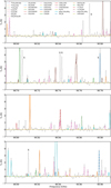 |
Fig. B.1 Fitted model for each molecule on top of the Band 3 data in gray. For readability, the y-axis limit was set to 5 K; however, no line was overestimated except those of methanol and one line of aGg′-(CH2OH)2, which are potentially optically thick. The lines that have an intensity higher than 2 K (i.e., detected at a ≳7 − 10σ level) but that were not identified are indicated by an “X”. |
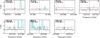 |
Fig. B.2 Lines of Ga-n-propanol and the model for its upper limit (6 × 1015 cm−2) in red. The symbols are the same as in Fig. 3. |
 |
Fig. B.3 Lines of G′Gg′gg′-Glycerol and the model for its upper limit (7 × 1015 cm−2) in red. The symbols are the same as in Fig. 3. |
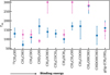 |
Fig. B.4 Excitation temperatures for molecules where a determination was possible. The species are ordered by their binding energies taken from Minissale et al. (2022) and Ligterink & Minissale (2023). The binding energy of the isotopologues was assumed to be the same as the major isotopologue. Band 3 results are shown in blue and Band 7 (PILS) in pink. PILS results with a fixed temperature are not shown. The temperatures for molecules from Jørgensen et al. (2018) are shown with either 300 ± 60 K or 125 ± 25 K depending on the group with which they were associated. |
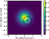 |
Fig. B.5 Two-dimensional Gaussian function with a total integration of one and a FWHM of 0.5″ (color scale). This was assumed as a typical emission distribution for COMs based on the results of PILS (e.g., Jørgensen et al. 2016). Two circular regions with radii of 0.25″ and 0.5″ are overplotted, representing beams of PILS (white) and Band 3 (black), respectively. The crosses show the peak position, 0.25″, and 0.5″ offset positions. |
Upper limits of non-detections.
Transitions of the species studied here in the data that have Eup < 1000 K and Aij > 10−9 s−1 (not all were detected).
References
- Agúndez, M., Loison, J. C., Hickson, K. M., et al. 2023, A&A, 673, A34 [NASA ADS] [CrossRef] [EDP Sciences] [Google Scholar]
- Bacmann, A., Taquet, V., Faure, A., Kahane, C., & Ceccarelli, C. 2012, A&A, 541, A12 [NASA ADS] [CrossRef] [EDP Sciences] [Google Scholar]
- Bacmann, A., Faure, A., & Berteaud, J. 2019, ACS Earth Space Chem., 3, 1000 [Google Scholar]
- Barone, V., Latouche, C., Skouteris, D., et al. 2015, MNRAS, 453, L31 Baskakov, O. I., Alekseev, E. A., Motiyenko, R. A., et al. 2006, J. Mol. Spectrosc., 240, 188 [NASA ADS] [CrossRef] [Google Scholar]
- Belloche, A., Müller, H. S. P., Menten, K. M., Schilke, P., & Comito, C. 2013, A&A, 559, A47 [NASA ADS] [CrossRef] [EDP Sciences] [Google Scholar]
- Belloche, A., Garrod, R. T., Müller, H. S. P., et al. 2019, A&A, 628, A10 [NASA ADS] [CrossRef] [EDP Sciences] [Google Scholar]
- Belloche, A., Maury, A. J., Maret, S., et al. 2020, A&A, 635, A198 [NASA ADS] [CrossRef] [EDP Sciences] [Google Scholar]
- Belloche, A., Garrod, R. T., Zingsheim, O., Müller, H. S. P., & Menten, K. M. 2022, A&A, 662, A110 [NASA ADS] [CrossRef] [EDP Sciences] [Google Scholar]
- Bergner, J. B., Öberg, K. I., Garrod, R. T., & Graninger, D. M. 2017, ApJ, 841, 120 [Google Scholar]
- Bianchi, E., López-Sepulcre, A., Ceccarelli, C., et al. 2022, ApJ, 928, L3 [NASA ADS] [CrossRef] [Google Scholar]
- Bisschop, S. E., Jørgensen, J. K., Bourke, T. L., Bottinelli, S., & van Dishoeck, E. F. 2008, A&A, 488, 959 [NASA ADS] [CrossRef] [EDP Sciences] [Google Scholar]
- Blake, G. A., Sutton, E. C., Masson, C. R., & Phillips, T. G. 1987, ApJ, 315, 621 [Google Scholar]
- Bocquet, R., Demaison, J., Cosléou, J., et al. 1999, J. Mol. Spectrosc., 195, 345 [NASA ADS] [CrossRef] [Google Scholar]
- Bøgelund, E. G., McGuire, B. A., Ligterink, N. F. W., et al. 2018, A&A, 615, A88 [Google Scholar]
- Booth, A. S., Walsh, C., Terwisscha van Scheltinga, J., et al. 2021, Nat. Astron., 5, 684 [NASA ADS] [CrossRef] [Google Scholar]
- Bouchez, A., Margulès, L., Motiyenko, R. A., et al. 2012, A&A, 540, A51 [NASA ADS] [CrossRef] [EDP Sciences] [Google Scholar]
- Brauer, C. S., Pearson, J. C., Drouin, B. J., & Yu, S. 2009, ApJS, 184, 133 [CrossRef] [Google Scholar]
- Brunken, N. G. C., Booth, A. S., Leemker, M., et al. 2022, A&A, 659, A29 [NASA ADS] [CrossRef] [EDP Sciences] [Google Scholar]
- Busch, L. A., Belloche, A., Garrod, R. T., Müller, H. S. P., & Menten, K. M. 2022, A&A, 665, A96 [NASA ADS] [CrossRef] [EDP Sciences] [Google Scholar]
- Butner, H. M., Charnley, S. B., Ceccarelli, C., et al. 2007, ApJ, 659, L137 [Google Scholar]
- Calcutt, H., Fiechter, M. R., Willis, E. R., et al. 2018a, A&A, 617, A95 [NASA ADS] [CrossRef] [EDP Sciences] [Google Scholar]
- Calcutt, H., Jørgensen, J. K., Müller, H. S. P., et al. 2018b, A&A, 616, A90 [NASA ADS] [CrossRef] [EDP Sciences] [Google Scholar]
- Cazaux, S., Tielens, A. G. G. M., Ceccarelli, C., et al. 2003, ApJ, 593, L51 [CrossRef] [Google Scholar]
- Ceccarelli, C., Bacmann, A., Boogert, A., et al. 2010, A&A, 521, L22 [NASA ADS] [CrossRef] [EDP Sciences] [Google Scholar]
- Ceccarelli, C., Codella, C., Balucani, N., et al. 2022, arXiv e-prints [arXiv:2206.13270] [Google Scholar]
- Cernicharo, J., Agúndez, M., Cabezas, C., et al. 2021, A&A, 649, L15 [EDP Sciences] [Google Scholar]
- Chen, Y., van Gelder, M. L., Nazari, P., et al. 2023, A&A, 678, A137 [NASA ADS] [CrossRef] [EDP Sciences] [Google Scholar]
- Christen, D., & Müller, H. S. P. 2003, Phys. Chem. Chem. Phys. (Incorp. Faraday Trans.), 5, 3600 [NASA ADS] [CrossRef] [Google Scholar]
- Christen, D., Coudert, L. H., Suenram, R. D., & Lovas, F. J. 1995, J. Mol. Spectrosc., 172, 57 [NASA ADS] [CrossRef] [Google Scholar]
- Christen, D., Coudert, L. H., Larsson, J. A., & Cremer, D. 2001, J. Mol. Spectrosc., 205, 185 [NASA ADS] [CrossRef] [Google Scholar]
- Chuang, K. J., Fedoseev, G., Qasim, D., et al. 2020, A&A, 635, A199 [NASA ADS] [CrossRef] [EDP Sciences] [Google Scholar]
- Chuang, K. J., Fedoseev, G., Scirè, C., et al. 2021, A&A, 650, A85 [NASA ADS] [CrossRef] [EDP Sciences] [Google Scholar]
- Chuang, K. J., Jäger, C., Krasnokutski, S. A., Fulvio, D., & Henning, T. 2022, ApJ, 933, 107 [CrossRef] [Google Scholar]
- Coletta, A., Fontani, F., Rivilla, V. M., et al. 2020, A&A, 641, A54 [NASA ADS] [CrossRef] [EDP Sciences] [Google Scholar]
- Collings, M. P., Anderson, M. A., Chen, R., et al. 2004, MNRAS, 354, 1133 [NASA ADS] [CrossRef] [Google Scholar]
- Coudert, L. H., Margulès, L., Vastel, C., et al. 2019, A&A, 624, A70 [NASA ADS] [CrossRef] [EDP Sciences] [Google Scholar]
- Coutens, A., Jørgensen, J. K., van der Wiel, M. H. D., et al. 2016, A&A, 590, L6 [NASA ADS] [CrossRef] [EDP Sciences] [Google Scholar]
- Coutens, A., Loison, J. C., Boulanger, A., et al. 2022, A&A, 660, L6 [NASA ADS] [CrossRef] [EDP Sciences] [Google Scholar]
- Creswell, R. A., & Schwendeman, R. H. 1974, Chem. Phys. Lett., 27, 521 [NASA ADS] [CrossRef] [Google Scholar]
- Creswell, R. A., Winnewisser, G., & Gerry, M. C. L. 1977, J. Mol. Spectrosc., 65, 420 [CrossRef] [Google Scholar]
- Dangoisse, D., Willemot, E., & Bellet, J. 1978, J. Mol. Spectrosc., 71, 414 [NASA ADS] [CrossRef] [Google Scholar]
- De Simone, M., Ceccarelli, C., Codella, C., et al. 2020, ApJ, 896, L3 [NASA ADS] [CrossRef] [Google Scholar]
- de Zafra, R. L. 1971, ApJ, 170, 165 [NASA ADS] [CrossRef] [Google Scholar]
- Dickens, J. E., Irvine, W. M., Ohishi, M., et al. 1997, ApJ, 489, 753 [NASA ADS] [CrossRef] [Google Scholar]
- Drozdovskaya, M. N., van Dishoeck, E. F., Jørgensen, J. K., et al. 2018, MNRAS, 476, 4949 [Google Scholar]
- Drozdovskaya, M. N., van Dishoeck, E. F., Rubin, M., Jørgensen, J. K., & Altwegg, K. 2019, MNRAS, 490, 50 [Google Scholar]
- Drozdovskaya, M. N., Coudert, L. H., Margulès, L., et al. 2022, A&A, 659, A69 [NASA ADS] [CrossRef] [EDP Sciences] [Google Scholar]
- Durig, J. R., Bucy, W. E., Wurrey, C. J., & Carreira, L. A. 1975, J. Phys. Chem., 79, 988 [CrossRef] [Google Scholar]
- Endres, C. P., Drouin, B. J., Pearson, J. C., et al. 2009, A&A, 504, 635 [NASA ADS] [CrossRef] [EDP Sciences] [Google Scholar]
- Fedoseev, G., Cuppen, H. M., Ioppolo, S., Lamberts, T., & Linnartz, H. 2015, MNRAS, 448, 1288 [NASA ADS] [CrossRef] [Google Scholar]
- Fedoseev, G., Chuang, K. J., Ioppolo, S., et al. 2017, ApJ, 842, 52 [Google Scholar]
- Fedoseev, G., Qasim, D., Chuang, K.-J., et al. 2022, ApJ, 924, 110 [NASA ADS] [CrossRef] [Google Scholar]
- Ferrer Asensio, J., Spezzano, S., Coudert, L. H., et al. 2023, A&A, 670, A177 [NASA ADS] [CrossRef] [EDP Sciences] [Google Scholar]
- Fukuyama, Y., Odashima, H., Takagi, K., & Tsunekawa, S. 1996, ApJS, 104, 329 [NASA ADS] [CrossRef] [Google Scholar]
- Garrod, R. T., Jin, M., Matis, K. A., et al. 2022, ApJS, 259, 1 [NASA ADS] [CrossRef] [Google Scholar]
- Gratier, P., Majumdar, L., Ohishi, M., et al. 2016, ApJS, 225, 25 [Google Scholar]
- Groner, P., Albert, S., Herbst, E., et al. 2002, ApJS, 142, 145 [NASA ADS] [CrossRef] [Google Scholar]
- Haykal, I., Motiyenko, R. A., Margulès, L., & Huet, T. R. 2013, A&A, 549, A96 [NASA ADS] [CrossRef] [EDP Sciences] [Google Scholar]
- Herbst, E., & van Dishoeck, E. F. 2009, ARA&A, 47, 427 [NASA ADS] [CrossRef] [Google Scholar]
- Hirose, C. 1974, ApJ, 189, L145 [NASA ADS] [CrossRef] [Google Scholar]
- Hirota, E., Sugisaki, R., Nielsen, C. J., & Sørensen, G. O. 1974, J. Mol. Spectrosc., 49, 251 [NASA ADS] [CrossRef] [Google Scholar]
- Hsu, S.-Y., Liu, S.-Y., Liu, T., et al. 2022, ApJ, 927, 218 [NASA ADS] [CrossRef] [Google Scholar]
- Ikeda, M., Ohishi, M., Nummelin, A., et al. 2001, ApJ, 560, 792 [Google Scholar]
- Ilyushin, V., Kryvda, A., & Alekseev, E. 2009, J. Mol. Spectrosc., 255, 32 [NASA ADS] [CrossRef] [Google Scholar]
- Ilyushin, V. V., Endres, C. P., Lewen, F., Schlemmer, S., & Drouin, B. J. 2013, J. Mol. Spectrosc., 290, 31 [NASA ADS] [CrossRef] [Google Scholar]
- Ilyushin, V. V., Müller, H. S. P., Jørgensen, J. K., et al. 2022, A&A, 658, A127 [NASA ADS] [CrossRef] [EDP Sciences] [Google Scholar]
- Ioppolo, S., Fedoseev, G., Chuang, K. J., et al. 2021, Nat. Astron., 5, 197 [NASA ADS] [CrossRef] [Google Scholar]
- Jaber, A. A., Ceccarelli, C., Kahane, C., & Caux, E. 2014, ApJ, 791, 29 [Google Scholar]
- Jacobsen, S. K., Jørgensen, J. K., van der Wiel, M. H. D., et al. 2018, A&A, 612, A72 [NASA ADS] [CrossRef] [EDP Sciences] [Google Scholar]
- Jiménez-Serra, I., Vasyunin, A. I., Caselli, P., et al. 2016, ApJ, 830, L6 [Google Scholar]
- Jiménez-Serra, I., Martín-Pintado, J., Rivilla, V. M., et al. 2020, Astrobiology, 20, 1048 [Google Scholar]
- Jiménez-Serra, I., Rodríguez-Almeida, L. F., Martín-Pintado, J., et al. 2022, A&A, 663, A181 [NASA ADS] [CrossRef] [EDP Sciences] [Google Scholar]
- Jones, B. M., Bennett, C. J., & Kaiser, R. I. 2011, ApJ, 734, 78 [Google Scholar]
- Jørgensen, J. K., Schöier, F. L., & van Dishoeck, E. F. 2002, A&A, 389, 908 [CrossRef] [EDP Sciences] [Google Scholar]
- Jørgensen, J. K., Bourke, T. L., Nguyen Luong, Q., & Takakuwa, S. 2011, A&A, 534, A100 [NASA ADS] [CrossRef] [EDP Sciences] [Google Scholar]
- Jørgensen, J. K., Favre, C., Bisschop, S. E., et al. 2012, ApJ, 757, L4 [Google Scholar]
- Jørgensen, J. K., van der Wiel, M. H. D., Coutens, A., et al. 2016, A&A, 595, A117 [Google Scholar]
- Jørgensen, J. K., Müller, H. S. P., Calcutt, H., et al. 2018, A&A, 620, A170 [Google Scholar]
- Jørgensen, J. K., Belloche, A., & Garrod, R. T. 2020, ARA&A, 58, 727 [Google Scholar]
- Kahane, C., Ceccarelli, C., Faure, A., & Caux, E. 2013, ApJ, 763, L38 [CrossRef] [Google Scholar]
- Kleiner, I., Lovas, F. J., & Godefroid, M. 1996, J. Phys. Chem. Ref. Data, 25, 1113 [CrossRef] [Google Scholar]
- Kryvda, A. V., Gerasimov, V. G., Dyubko, S. F., Alekseev, E. A., & Motiyenko, R. A. 2009, J. Mol. Spectrosc., 254, 28 [NASA ADS] [CrossRef] [Google Scholar]
- Kukolich, S. G., & Nelson, A. C. 1971, Chem. Phys. Lett., 11, 383 [NASA ADS] [CrossRef] [Google Scholar]
- Lauvergnat, D., Coudert, L. H., Klee, S., & Smirnov, M. 2009, J. Mol. Spectrosc., 256, 204 [NASA ADS] [CrossRef] [Google Scholar]
- Ligterink, N. F. W., & Minissale, M. 2023, A&A, 676, A80 [NASA ADS] [CrossRef] [EDP Sciences] [Google Scholar]
- Ligterink, N. F. W., El-Abd, S. J., Brogan, C. L., et al. 2020, ApJ, 901, 37 [Google Scholar]
- Ligterink, N. F. W., Ahmadi, A., Coutens, A., et al. 2021, A&A, 647, A87 [NASA ADS] [CrossRef] [EDP Sciences] [Google Scholar]
- López-Sepulcre, A., Sakai, N., Neri, R., et al. 2017, A&A, 606, A121 [NASA ADS] [CrossRef] [EDP Sciences] [Google Scholar]
- Lykke, J. M., Coutens, A., Jørgensen, J. K., et al. 2017, A&A, 597, A53 [NASA ADS] [CrossRef] [EDP Sciences] [Google Scholar]
- Mallinson, P., & Fayt, A. 1976, Mol. Phys., 32, 473 [NASA ADS] [CrossRef] [Google Scholar]
- Manigand, S., Calcutt, H., Jørgensen, J. K., et al. 2019, A&A, 623, A69 [NASA ADS] [CrossRef] [EDP Sciences] [Google Scholar]
- Manigand, S., Jørgensen, J. K., Calcutt, H., et al. 2020, A&A, 635, A48 [NASA ADS] [CrossRef] [EDP Sciences] [Google Scholar]
- Manigand, S., Coutens, A., Loison, J. C., et al. 2021, A&A, 645, A53 [NASA ADS] [CrossRef] [EDP Sciences] [Google Scholar]
- Margulès, L., Motiyenko, R. A., Ilyushin, V. V., & Guillemin, J. C. 2015, A&A, 579, A46 [NASA ADS] [CrossRef] [EDP Sciences] [Google Scholar]
- Margulès, L., McGuire, B. A., Senent, M. L., et al. 2017, A&A, 601, A50 [NASA ADS] [CrossRef] [EDP Sciences] [Google Scholar]
- Margulès, L., Coutens, A., Ligterink, N. F. W., et al. 2023, MNRAS, 524, 1211 [CrossRef] [Google Scholar]
- Maureira, M. J., Pineda, J. E., Segura-Cox, D. M., et al. 2020, ApJ, 897, 59 [NASA ADS] [CrossRef] [Google Scholar]
- McClure, M. K., Rocha, W. R. M., Pontoppidan, K. M., et al. 2023, Nat. Astron., 7, 431 [NASA ADS] [CrossRef] [Google Scholar]
- McGuire, B. A. 2022, ApJS, 259, 30 [NASA ADS] [CrossRef] [Google Scholar]
- McGuire, B. A., Burkhardt, A. M., Loomis, R. A., et al. 2020, ApJ, 900, L10 [Google Scholar]
- McGuire, B. A., Loomis, R. A., Burkhardt, A. M., et al. 2021, Science, 371, 1265 [Google Scholar]
- McMullin, J. P., Waters, B., Schiebel, D., Young, W., & Golap, K. 2007, in ASP Conf. Ser., 376, Astronomical Data Analysis Software and Systems XVI, eds. R. A. Shaw, F. Hill, & D. J. Bell, 127 [NASA ADS] [Google Scholar]
- McNaughton, D., Jahn, M. K., Travers, M. J., et al. 2018, MNRAS, 476, 5268 [CrossRef] [Google Scholar]
- Medcraft, C., Thompson, C. D., Robertson, E. G., Appadoo, D. R. T., & McNaughton, D. 2012, ApJ, 753, 18 [Google Scholar]
- Milam, S. N., Savage, C., Brewster, M. A., Ziurys, L. M., & Wyckoff, S. 2005, ApJ, 634, 1126 [Google Scholar]
- Minissale, M., Aikawa, Y., Bergin, E., et al. 2022, ACS Earth Space Chem., 6, 597 [NASA ADS] [CrossRef] [Google Scholar]
- Motiyenko, R. A., Tercero, B., Cernicharo, J., & Margulès, L. 2012, A&A, 548, A71 [NASA ADS] [CrossRef] [EDP Sciences] [Google Scholar]
- Müller, H. S. P., & Christen, D. 2004, J. Mol. Spectrosc., 228, 298 [CrossRef] [Google Scholar]
- Müller, H. S. P., Thorwirth, S., Roth, D. A., & Winnewisser, G. 2001, A&A, 370, L49 [Google Scholar]
- Müller, H. S. P., Schlöder, F., Stutzki, J., & Winnewisser, G. 2005, J. Mol. Struct., 742, 215 [Google Scholar]
- Müller, H. S. P., Belloche, A., Xu, L.-H., et al. 2016, A&A, 587, A92 [NASA ADS] [CrossRef] [EDP Sciences] [Google Scholar]
- Müller, H. S. P., Jørgensen, J. K., Guillemin, J.-C., Lewen, F., & Schlemmer, S. 2023a, MNRAS, 518, 185 [Google Scholar]
- Müller, H. S. P., Jørgensen, J. K., Guillemin, J.-C., Lewen, F., & Schlemmer, S. 2023b, J. Mol. Spectrosc., 394, 111777 [CrossRef] [Google Scholar]
- Murillo, N. M., Hsieh, T. H., & Walsh, C. 2022a, A&A, 665, A68 [NASA ADS] [CrossRef] [EDP Sciences] [Google Scholar]
- Murillo, N. M., van Dishoeck, E. F., Hacar, A., Harsono, D., & Jørgensen, J. K. 2022b, A&A, 658, A53 [NASA ADS] [CrossRef] [EDP Sciences] [Google Scholar]
- Nazari, P., van Gelder, M. L., van Dishoeck, E. F., et al. 2021, A&A, 650, A150 [EDP Sciences] [Google Scholar]
- Nazari, P., Meijerhof, J. D., van Gelder, M. L., et al. 2022a, A&A, 668, A109 [NASA ADS] [CrossRef] [EDP Sciences] [Google Scholar]
- Nazari, P., Tabone, B., Rosotti, G. P., et al. 2022b, A&A, 663, A58 [NASA ADS] [CrossRef] [EDP Sciences] [Google Scholar]
- Nazari, P., Tabone, B., & Rosotti, G. P. 2023a, A&A, 671, A107 [NASA ADS] [CrossRef] [EDP Sciences] [Google Scholar]
- Nazari, P., Tabone, B., Rosotti, G. P., & van Dishoeck, E. F. 2023b, A&A, submitted [arXiv:2404.10045] [Google Scholar]
- Nazari, P., Tabone, B., van’t Hoff, M. L. R., Jørgensen, J. K., & van Dishoeck, E. F. 2023c, ApJ, 951, L38 [NASA ADS] [CrossRef] [Google Scholar]
- Nummelin, A., Dickens, J. E., Bergman, P., et al. 1998, A&A, 337, 275 [NASA ADS] [PubMed] [Google Scholar]
- Öberg, K. I., Garrod, R. T., van Dishoeck, E. F., & Linnartz, H. 2009, A&A, 504, 891 [NASA ADS] [CrossRef] [EDP Sciences] [Google Scholar]
- Öberg, K. I., Boogert, A. C. A., Pontoppidan, K. M., et al. 2011, ApJ, 740, 109 [Google Scholar]
- Öberg, K. I., Guzmán, V. V., Furuya, K., et al. 2015, Nature, 520, 198 [Google Scholar]
- Ordu, M. H., Zingsheim, O., Belloche, A., et al. 2019, A&A, 629, A72 [NASA ADS] [CrossRef] [EDP Sciences] [Google Scholar]
- Pearson, J. C., Sastry, K. V. L. N., Herbst, E., & De Lucia, F. C. 1994, ApJS, 93, 589 [Google Scholar]
- Pearson, J. C., Brauer, C. S., & Drouin, B. J. 2008, J. Mol. Spectrosc., 251, 394 [NASA ADS] [CrossRef] [Google Scholar]
- Pearson, J. C., Yu, S., & Drouin, B. J. 2012, J. Mol. Spectrosc., 280, 119 [NASA ADS] [CrossRef] [Google Scholar]
- Perrin, A., Flaud, J. M., Bakri, B., et al. 2002, J. Mol. Spectrosc., 216, 203 [NASA ADS] [CrossRef] [Google Scholar]
- Persson, M. V., Harsono, D., Tobin, J. J., et al. 2016, A&A, 590, A33 [NASA ADS] [CrossRef] [EDP Sciences] [Google Scholar]
- Persson, M. V., Jørgensen, J. K., Müller, H. S. P., et al. 2018, A&A, 610, A54 [NASA ADS] [CrossRef] [EDP Sciences] [Google Scholar]
- Pickett, H. M., Poynter, R. L., Cohen, E. A., et al. 1998, J. Quant. Spec. Radiat. Transf., 60, 883 [Google Scholar]
- Qasim, D., Fedoseev, G., Chuang, K. J., et al. 2019a, A&A, 627, A1 [NASA ADS] [CrossRef] [EDP Sciences] [Google Scholar]
- Qasim, D., Fedoseev, G., Lamberts, T., et al. 2019b, ACS Earth Space Chem., 3, 986 [NASA ADS] [CrossRef] [Google Scholar]
- Requena-Torres, M. A., Martín-Pintado, J., Rodríguez-Franco, A., et al. 2006, A&A, 455, 971 [NASA ADS] [CrossRef] [EDP Sciences] [Google Scholar]
- Requena-Torres, M. A., Martín-Pintado, J., Martín, S., & Morris, M. R. 2008, ApJ, 672, 352 [Google Scholar]
- Rivilla, V. M., Beltrán, M. T., Cesaroni, R., et al. 2017, A&A, 598, A59 [NASA ADS] [CrossRef] [EDP Sciences] [Google Scholar]
- Rivilla, V. M., Jiménez-Serra, I., Martín-Pintado, J., et al. 2021, PNAS, 118, e2101314118 [NASA ADS] [CrossRef] [Google Scholar]
- Rivilla, V. M., Jiménez-Serra, I., Martín-Pintado, J., et al. 2022, Front. Astron. Space Sci., 9, 876870 [NASA ADS] [CrossRef] [Google Scholar]
- Rocha, W. R. M., Rachid, M. G., Olsthoorn, B., et al. 2022, A&A, 668, A63 [NASA ADS] [CrossRef] [EDP Sciences] [Google Scholar]
- Rodríguez-Almeida, L. F., Jiménez-Serra, I., Rivilla, V. M., et al. 2021, ApJ, 912, L11 [Google Scholar]
- Sánchez-Monge, Á., Schilke, P., Ginsburg, A., Cesaroni, R., & Schmiedeke, A. 2018, A&A, 609, A101 [Google Scholar]
- Schutte, W. A., Boogert, A. C. A., Tielens, A. G. G. M., et al. 1999, A&A, 343, 966 [NASA ADS] [Google Scholar]
- Scibelli, S., & Shirley, Y. 2020, ApJ, 891, 73 [NASA ADS] [CrossRef] [Google Scholar]
- Taniguchi, K., Sanhueza, P., Olguin, F. A., et al. 2023, ApJ, 950, 57 [CrossRef] [Google Scholar]
- Taquet, V., van Dishoeck, E. F., Swayne, M., et al. 2018, A&A, 618, A11 [NASA ADS] [CrossRef] [EDP Sciences] [Google Scholar]
- Theulé, P., Duvernay, F., Danger, G., et al. 2013, Adv. Space Res., 52, 1567 [CrossRef] [Google Scholar]
- Thorwirth, S., Müller, H. S. P., & Winnewisser, G. 2000, J. Mol. Spectrosc., 204, 133 [NASA ADS] [CrossRef] [Google Scholar]
- van Dishoeck, E. F., Blake, G. A., Jansen, D. J., & Groesbeck, T. D. 1995, ApJ, 447, 760 [Google Scholar]
- van Gelder, M. L., Tabone, B., Tychoniec, Ł., et al. 2020, A&A, 639, A87 [NASA ADS] [CrossRef] [EDP Sciences] [Google Scholar]
- van Gelder, M. L., Jaspers, J., Nazari, P., et al. 2022a, A&A, 667, A136 [NASA ADS] [CrossRef] [EDP Sciences] [Google Scholar]
- van Gelder, M. L., Nazari, P., Tabone, B., et al. 2022b, A&A, 662, A67 [NASA ADS] [CrossRef] [EDP Sciences] [Google Scholar]
- Vastel, C., Bottinelli, S., Caux, E., Glorian, J. M., & Boiziot, M. 2015, in SF2A-2015: Proceedings of the Annual meeting of the French Society of Astronomy and Astrophysics, 313 [Google Scholar]
- Vazart, F., Ceccarelli, C., Balucani, N., Bianchi, E., & Skouteris, D. 2020, MNRAS, 499, 5547 [Google Scholar]
- Walsh, C., Loomis, R. A., Öberg, K. I., et al. 2016, ApJ, 823, L10 [NASA ADS] [CrossRef] [Google Scholar]
- Walters, A., Schäfer, M., Ordu, M. H., et al. 2015, J. Mol. Spectrosc., 314, 6 [NASA ADS] [CrossRef] [Google Scholar]
- Winnewisser, M., Winnewisser, B. P., Stein, M., et al. 2002, J. Mol. Spectrosc., 216, 259 [NASA ADS] [CrossRef] [Google Scholar]
- Wootten, A. 1989, ApJ, 337, 858 [NASA ADS] [CrossRef] [Google Scholar]
- Xu, L.-H., & Lovas, F. J. 1997, J. Phys. Chem. Ref. Data, 26, 17 [Google Scholar]
- Yamada, K. M. T., Moravec, A., & Winnewisser, G. 1995, Z. Naturf. A, 50, 1179 [NASA ADS] [CrossRef] [Google Scholar]
- Yang, Y.-L., Sakai, N., Zhang, Y., et al. 2021, ApJ, 910, 20 [Google Scholar]
- Yang, Y.-L., Green, J. D., Pontoppidan, K. M., et al. 2022, ApJ, 941, L13 [NASA ADS] [CrossRef] [Google Scholar]
- Zakharenko, O., Ilyushin, V. V., Lewen, F., et al. 2019, A&A, 629, A73 [NASA ADS] [CrossRef] [EDP Sciences] [Google Scholar]
- Zeng, S., Quénard, D., Jiménez-Serra, I., et al. 2019, MNRAS, 484, L43 [Google Scholar]
- Zeng, S., Rivilla, V. M., Jiménez-Serra, I., et al. 2023, MNRAS, 523, 1448 [NASA ADS] [CrossRef] [Google Scholar]
All Tables
Fitted parameters for detected and tentatively detected Band 3 species toward IRAS 16293 B.
Transitions of the species studied here in the data that have Eup < 1000 K and Aij > 10−9 s−1 (not all were detected).
All Figures
|
Fig. 1 Spectrum of IRAS16293 B Band 3 data for the continuum window. A few strong lines are highlighted; for the full line identification and fitting, readers can refer to Fig. B.1. We note that “X” indicates a line that has not been identified yet and that was not (fully) fitted with the considered molecules for this work. The spectrum of IRAS16293 B is line rich even at ALMA Band 3 wavelengths (~3 mm). |
| In the text | |
|
Fig. 2 Column density ratios of detected species and upper limits with respect to methanol. Left: column density ratios for the detected species with respect to methanol for our Band 3 data (blue). The same ratios from PILS in Band 7 (pink) are also shown for comparison (see the text for references). The hollow symbols show the species that only have one detected line. Right: ratios of the upper limits measured in this work (Table B.1) with respect to methanol. In both panels, the species are ordered from left to right by increasing Band 3 ratios with respect to methanol. |
| In the text | |
|
Fig. 3 Lines of g-Isopropanol and the model for its upper limit in red dashed lines (1.5 × 1016 cm−2). Gray is the data and cyan is the total fitted model from the detected and tentatively detected species. The vertical dotted lines show the transition frequency of each line. The Eup and Aij are printed in the top left of each panel. The line that was used to find the 3σ upper limit is indicated by an “X” in the top right. The horizontal dashed lines show the 3σ level. Only lines with Aij > 10−6 s−1 and Eup < 300 K are shown. |
| In the text | |
|
Fig. 4 Continuum optical depth as a function of temperature at the peak of the continuum (dashed) and the 0.5″ offset position where the spectrum was extracted (solid line). Blue shows the optical depth for the Band 3 continuum at a frequency of ~91 GHz and pink shows the PILS continuum at a frequency of ~348.815 GHz. |
| In the text | |
|
Fig. 5 Column density of the various molecules from the ALMA Band 7 observations (PILS; ~345 GHz) as a function of those from Band 3 (~100 GHz). Beam dilution was corrected for the column densities in this figure. Dashed lines present where the values of the y-axis are the same as the values of the x-axis, where they are ten times higher and ten times lower than the values of the x-axis. |
| In the text | |
|
Fig. 6 Ratio between Band 3 and PILS column density ratios with respect to methanol (i.e., the ratio of blue to pink from the left panel of Fig. 2). The horizontal dashed line indicates where the ratio between Band 3 and PILS are the same. The shaded gray area indicates the region with a factor of two difference between Band 3 and PILS results. The species are ordered in the same way as in the left panel of Fig. 2. The hollow symbols show the species that have only one detected line. |
| In the text | |
|
Fig. B.1 Fitted model for each molecule on top of the Band 3 data in gray. For readability, the y-axis limit was set to 5 K; however, no line was overestimated except those of methanol and one line of aGg′-(CH2OH)2, which are potentially optically thick. The lines that have an intensity higher than 2 K (i.e., detected at a ≳7 − 10σ level) but that were not identified are indicated by an “X”. |
| In the text | |
|
Fig. B.2 Lines of Ga-n-propanol and the model for its upper limit (6 × 1015 cm−2) in red. The symbols are the same as in Fig. 3. |
| In the text | |
|
Fig. B.3 Lines of G′Gg′gg′-Glycerol and the model for its upper limit (7 × 1015 cm−2) in red. The symbols are the same as in Fig. 3. |
| In the text | |
|
Fig. B.4 Excitation temperatures for molecules where a determination was possible. The species are ordered by their binding energies taken from Minissale et al. (2022) and Ligterink & Minissale (2023). The binding energy of the isotopologues was assumed to be the same as the major isotopologue. Band 3 results are shown in blue and Band 7 (PILS) in pink. PILS results with a fixed temperature are not shown. The temperatures for molecules from Jørgensen et al. (2018) are shown with either 300 ± 60 K or 125 ± 25 K depending on the group with which they were associated. |
| In the text | |
|
Fig. B.5 Two-dimensional Gaussian function with a total integration of one and a FWHM of 0.5″ (color scale). This was assumed as a typical emission distribution for COMs based on the results of PILS (e.g., Jørgensen et al. 2016). Two circular regions with radii of 0.25″ and 0.5″ are overplotted, representing beams of PILS (white) and Band 3 (black), respectively. The crosses show the peak position, 0.25″, and 0.5″ offset positions. |
| In the text | |
Current usage metrics show cumulative count of Article Views (full-text article views including HTML views, PDF and ePub downloads, according to the available data) and Abstracts Views on Vision4Press platform.
Data correspond to usage on the plateform after 2015. The current usage metrics is available 48-96 hours after online publication and is updated daily on week days.
Initial download of the metrics may take a while.