| Issue |
A&A
Volume 686, June 2024
|
|
|---|---|---|
| Article Number | A20 | |
| Number of page(s) | 27 | |
| Section | Catalogs and data | |
| DOI | https://doi.org/10.1051/0004-6361/202346439 | |
| Published online | 27 May 2024 | |
Characterizing B stars from Kepler/K2 Campaign 11
Optical analysis and seismic diagnostics
1
Observatório Nacional, MCTI,
20921-400
Rio de Janeiro, RJ, Brazil
e-mail: This email address is being protected from spambots. You need JavaScript enabled to view it.
2
Instituto de Astronomia, Geofísica e Ciências Atmosféricas, Universidade de São Paulo,
05509-090
São Paulo, SP, Brazil
e-mail: This email address is being protected from spambots. You need JavaScript enabled to view it.
3
Universidade Estadual de Ponta Grossa,
84030-900
Ponta Grossa, PR, Brazil
4
Laboratório Nacional de Astrofísica,
Rua Estados Unidos 154,
37504-364
Itajubá, MG, Brazil
5
Institute for Astronomy, University of Hawaii,
Maui, HI
96768, USA
6
W. W. Hansen Experimental Physics Laboratory, Stanford University,
Stanford, CA
94305, USA
Received:
17
March
2023
Accepted:
18
September
2023
Abstract
Aims. In this study, we analyze 122 B-type star candidates observed during Campaign 11 of the Kepler/K2 mission to investigate their variability and pulsation characteristics. A subset of 45 B star candidates was observed during the Kepler/K2 mission’s Campaign 11 between September and December 2016. Our analyses aim to gain a deeper understanding of the physical characteristics of these massive stars. Our methods involve both spectroscopy and seismology. The spectroscopic analysis was performed through mediumresolution blue spectra, which also allowed us to perform a spectral classification of the objects. Our results will contribute to the ongoing effort to expand our knowledge of variable B stars and the processes that drive their variability.
Methods. We used the iterative prewhitening and wavelet frequency searching algorithms to analyze the light curves to identify the different types of variability in the data. The frequencies were carefully chosen based on the signal-to-noise ratio and the magnitude of errors. We applied spectroscopic analysis techniques to enhance our understanding of the observed stars, including SME and MESA algorithms. A spectral classification was performed based on the observed spectra. The resulting astrophysical parameters were compared to Gaia mission data. Additionally, a seismology technique was applied to determine the average internal rotation frequency (vrot) and buoyancy travel time (P0) for selected stars in the sample.
Results. We detected several types of variability among the B-type stars, including slowly pulsating B (SPB) stars, hybrid pulsators showing both β Cep and SPB pulsations, stars with stochastic low-frequency (SLF) variability, Maia variables, and SPB/Maia hybrids. Their positions in our Gaia and classical HR diagrams are compatible with the theoretical expectations. We also found stars exhibiting variability attributed to binarity and rotation. We determined the physical characteristics for 45 of our targets and conducted a seismic analysis for 14 objects. Two SPB/Maia stars show internal velocities comparable to those of fast SPB stars. The derived average rotation frequencies, vrot, for these 14 stars lie between the critical vcritRoche and the minimal frequency values of vlimrot implied by the υ sin i measured from the spectra.
Conclusions. Our analysis classified 41 stars as SPB stars and attributed the primary variability of 53 objects to binarity, rotation, or both. We identified five stars as Maia/fast-rotating SPB variables. Two stars were classified as hybrid SPB/β Cep pulsators, and one as a β Cep binary. Thirteen stars exhibited prominent, low-frequency power excess, indicating SLF variability. Additionally, we found a positive correlation between the dominant fg frequency and the internal average rotation frequency.
Key words: techniques: spectroscopic / stars: fundamental parameters / stars: massive / stars: oscillations
© The Authors 2024
 Open Access article, published by EDP Sciences, under the terms of the Creative Commons Attribution License (https://creativecommons.org/licenses/by/4.0), which permits unrestricted use, distribution, and reproduction in any medium, provided the original work is properly cited.
This article is published in open access under the Subscribe to Open model. This email address is being protected from spambots. You need JavaScript enabled to view it. to support open access publication.
1 Introduction
Stars are undoubtedly the main players in our Universe. As described in Aerts et al. (2010), the chemical enrichment of galaxies, with all elements heavier than lithium, began in the interior of stars through nuclear fusion and has continued ever since. Stars bathe the interstellar medium with photon energy, playing an essential role in forming new stars and contributing to creating molecules essential for life. Lastly, stars serve as sources of the Universe’s dynamics and trace its gravitational behavior to an enormous extent. Therefore, understanding stars is essential in the field of astrophysics.
Variable stars serve as privileged laboratories for studying stellar physics and evolution. They offer additional parameters not available from non-variable stars, such as amplitudes and timescales. These parameters provide unique information that can be compared with theoretical models, leading to their improvement. For an extensive text on variable stars, we refer to Percy (2007). For more recent texts on the subject, including space data analysis, we refer to works such as Alexeev (2017) and Debosscher et al. (2007, 2009, 2011). This paper is focused on the various types of variable stars under investigation, elaborated upon in Sect. 4.
Recent advancements in space-based photometry using long time-series data have significantly improved our understanding of stellar interiors. Missions such as MOST (Walker et al. 2003), CoRoT (Viard et al. 2006), BRITE (Weiss et al. 2014), Kepler (Borucki et al. 2009), Kepler/K2 (Howell et al. 2014), and TESS (Ricker et al. 2015) have provided a wealth of high-precision, high-cadence data that have enabled the use of asteroseismology to probe the internal structure of stars. Analyzing stellar oscillations through asteroseismology represents a significantly powerful approach to extending our grasp of stellar structure properties and evolution models. This advancement is estimated at least one order of magnitude, as stated by Aerts et al. (2010). Therefore, asteroseismic modeling can be considered the ultimate objective of variability photometry investigations from space. These studies have revolutionized asteroseismological analyses by providing extensive databases spanning several years, thereby significantly enhancing the accuracy of observed frequency determinations. Many authors have presented asteroseismic analyses of B stars observed during the Kepler and K2 missions. Notable works in this area include Michielsen et al. (2021); Moravveji et al. (2015, 2016); Pâpics et al. (2017); Pedersen et al. (2021b); Szewczuk & Daszyńska-Daszkiewicz (2018); Szewczuk et al. (2021, 2022).
Slowly pulsating B (SPB) stars are mid to late B-type objects with effective temperatures ranging from ~ 10 000 to 19 000 K and masses typically between 2.5 and 8 M⊙. These stars exhibit high-order (n ≫ ℓ) gravity modes (g-modes) of non-radial pulsation, which are driven by the buoyancy force and excited by the κ mechanism (Dziembowski et al. 1993; Aerts et al. 2010, and references therein). In this mass range, a main-sequence star has a convective core, where nuclear fusion occurs, surrounded by a radiative envelope where the pulsations are trapped (Grotsch-Noels et al. 2016).
Ground-based detections of variability in the period range of 0.3–5 day−1 for SPB stars had proven challenging until the advent of space observations with high-precision uninterrupted photometry, marking a breakthrough in detecting non-radial pulsations in these stars.
In order to expand the number of observed B-type stars from space and better understand their variability classes, we proposed observing a sample of B stars during Campaign 11 of the K2 mission. These stars have not been studied as extensively as those from the original mission. We thoroughly analyzed the photometric data for 122 B-type star candidates in light of recent literature. We obtained spectroscopic data from ground-based observations for 45 stars in our sample, which provided valuable insights into the properties and characteristics of these stars, deepening our understanding of their nature.
Our sample includes a diverse range of B-type stars, including a small number of early-A and late-O type stars. The performed variability analysis revealed that the dominant group of pulsators were SPB stars. Additionally, many stars exhibited variations in their light curves due to rotation or binarity. A big fraction of stars showed indications of low-frequency variability (SLF, see Sect. 4.4). A small number of hybrid β Cep/SPB pulsators were also identified.
We also derived astrophysical parameters for 45 stars through spectroscopic analysis and performed a seismic analysis for fourteen targets. Our seismic analysis benefits from using the same frequencies used to classify the variability of our sample, enhancing the robustness of the results. By combining the spectroscopic and seismic studies, we explored the internal structure of the B star candidates, sought information on their evolutionary status and compared their assigned variability types with theoretical predictions. Our results showed that most of the B star candidates in our sample exhibited SPB-like pulsations consistent with their effective temperatures and masses. This paper provides an overview of the ground-based observations, including the data reduction and analysis procedures and the seismic and spectroscopic analyses.
This paper is organized as follows. Section 2 provides a detailed description of the data used in this study. Section 3 presents the results of the performed frequency analysis. The classification of the frequency spectra according to their variability characteristics is presented in Sect. 4. Section 5 provides an overview of the ground-based observations including the instrument setup, determination of stellar parameters through spectral synthesis and evolution models, and the method used for measuring projected rotational velocities. Section 6 discusses how to use g-modes to probe the interior of B stars. Section 7 presents a seismic method for calculating vrot and P0 values and presents the results, including identifying and characterizing pulsation modes and their associated frequencies. We also examine correlations between spectroscopic and seismic parameters in Sect. 8. Finally, in Sect. 9, we summarize our findings and discuss the implications of our study for understanding B-type stars.
2 Kepler and Gaia data
The original Kepler mission was designed to monitor the light fluxes of over a hundred thousand stars in a single patch of the sky in the Cygnus-Lyra region using a 1.4 m primary mirror and 42 CCDs integrated simultaneously (Van Cleve & Caldwell 2016). The mission successfully discovered thousands of new exoplanets, but the failure of two reaction wheels in May 2013 hindered the spacecraft’s ability to observe the original field stably. The K2 follow-on mission was developed as a solution, using the two remaining reaction wheels and solar radiation pressure to observe fields near the ecliptic for about 80 days per field (Van Cleve & Bryson 2017). Due to data storage and capacity constraints, most targets were observed with a 30 min or long cadence and a short mode of 1 min was reserved for selected targets.
During K2 Campaign 11, 122 B-type star candidates from our Guest Observer proposition were observed for 71 days between September and December 2016. The stars chosen for observation were of O9–B–A0 spectral types selected from the SIMBAD database. However, the campaign was divided into two segments due to an error in the initial roll-angle used to minimize solar torque on the spacecraft. The measurements were taken using a single, wide filter that overlapped with the B, V, R, and I Johnson filters. The measurements for this paper were taken at a 30-min cadence among 32 884 long cadence targets in Campaign 11.
In Fig. 1, we present the color-absolute-magnitude diagram (caMD) of our K2 Campaign 11 star sample using data from Data Release 3 (DR3) of the Gaia mission (Gaia Collaboration 2019, 2023b). The G-band absolute magnitude is calculated using the formula MG = G + 5 – 5 log10 r – AG, where G is the G-band apparent magnitude, r is the distance, and AG is the line-of-sight extinction in the G-band. The photogeometric distances used are those published by Bailer-Jones et al. (2021), also based on DR3 parallaxes and magnitudes. We also used the GALExtin service (Amôres et al. 2021) to obtain our targets’ 3D maps of extinction and reddening, using their coordinates and distances as well as their error bars. For most targets, extinction values were taken from Chen et al. (2019). The map from Green et al. (2019) was used for targets not covered by Chen et al. (2019), and the coefficients of these authors were used to convert from the Pan-STARRS1 to the Gaia color system. A few targets were not covered by both maps and for those targets, we used AG from Gaia DR3.
The colored symbols in Fig. 1 represent the stars’ variability types. Our classification method is described in Sect. 4. In the background of Fig. 1, we plot 200 000 stars observed by Gaia and Kepler for reference, highlighting the positions of the main sequence and the red clump. The evolutionary tracks of MIST (MESA Isochrones and Stellar Tracks) for 2, 4, and 8 M⊙ and the Sun’s position are also indicated (Dotter 2016). Most of the stars in our sample have locations consistent with spectral types B to A and luminosity classes I through V.
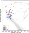 |
Fig. 1 Observational HR Gaia color-magnitude diagram of OBA stars from Campaign 11 of the K2 mission. On the x-axis the Gaia colour is shown, which is the difference in magnitude between the star’s measurement in the blue and red passbands. The y-axis gives the G-band absolute magnitude of the stars. The type of variability is indicate by different colours in the inset. The horizontal error bars represents primarily the uncertainty in the reddening of the stars (Amôres et al. 2021). The vertical error bar results from the sum of the distance uncertainty (Bailer-Jones et al. 2021) and the extinction uncertainty (Amôres et al. 2021). The background of the diagram is populated with gray points, representing 200 000 stars that are used to mark the main sequence and red clump regions, using data from Gaia Collaboration (2018). Evolutionary tracks of MIST for 2, 4, and 8 M⊙ and the position of the Sun as calculated by Casagrande & VandenBerg (2018) are also shown. |
3 Light curves and frequency spectra
The light curves provided by NASA’s Ames Research Center go through a three-step pipeline. The first step is the Calibration (CAL) module, where pixel-level calibrations are performed, such as bias, dark, gain, and flat-field, among others (Caldwell et al. 2010; Clarke et al. 2017). Next, the photometric analysis module ensures that the light curve data are accurate and reliable by applying various calibration techniques to the raw data (e.g., cosmic ray cleaning, background removal, astrometric solution and the aperture photometry, Morris et al. 2017).
The last step in the Kepler Science Pipeline is the Pre-search Data Conditioning (PDC). This complex step tries to remove systematic errors of two kinds using ancillary spacecraft data: 1) by searching and evaluating correlations between the detected flux and the error sources from the telescope and spacecraft systems, and 2) within the CCD itself, correcting for thermal gradients and consequent changes in focus or oscillations of the target centroid in the CCD plane, at pixel and subpixel level (Smith et al. 2017). The pipeline documentation warns that this step may introduce noise for complex light curves.
Lastly, while highly effective for optimal planet transit detection, it is essential to note that the PDC module may not be ideal for studying pulsations in hot pulsating stars. The module is primarily designed to eliminate systematic trends, discontinuities, and outliers, which could inadvertently remove or distort the pulsation signals of these stars. These unwanted side effects were significantly reduced after the adoption of the Bayesian maximum a posteriori approach to cotrending (PDC-MAP) on Kepler SOC version 8.0 and later (Stumpe et al. 2012), as the data used in this paper. Very long-period signals and brightness changes are still strongly affected but outside our analysis’s variability domains.
The standard masks automatically defined by the K2 pipeline were examined, and custom masks were defined for ten targets to avoid potential contamination from other sources. The custom masks were defined using the PYKE tool, and new light curves were extracted from the TPFs (Target Pixels File) provided by the MAST archive. It is only for EPIC 225962122 that the custom mask definition displays a significant effect due to light contamination from a nearby bright star. A standard light curve was obtained from the MAST data archive for all other targets.
The light curves were then corrected for systematic errors using K2SC (Aigrain et al. 2016, K2 Systematic Correction), which is intended to minimize the jitter effect on the data. In particular, K2SC employs a Gaussian process to correlate the star’s two-dimensional positional vector in the CCD with its light variability. This approach involves using a covariant function between pairs of observables, with the kernel of this function containing additive terms that allow for the separation of jitter-related systematics from astrophysical variability. The K2SC method was found to have performance equivalent to the K2SFf (K2 self-flatfielding) method from Vanderburg & Johnson (2014) but was considered more suitable for studies of stellar variability. Additionally, K2SC considers the inter-pixel and intra-pixel sensitivity variations between stars, which can result in different behavior even between similar stars close to the CCD (White et al. 2017). As a result, the functional form of the correction can vary from one star to another, making it a more robust method for correcting systematic errors in K2 data.
Signal detection methods such as the CLEANEST (Foster 1995) algorithm and the Lomb-Scargle (Scargle 1982) peri-odogram are used for time series data analysis, assuming that the data only contain white noise. However, in practice, the data often include additional noise sources, such as color noise, which can introduce bias and spectral leakage. Therefore, we employed a prewhitening technique to extract and study the properties of individual periodic components or frequencies on the time series. By removing the dominant signals, the prewhitened data allow for a more precise identification and analysis of the remaining signals or residuals.
In this work, we used the iterative prewhitening method described by Degroote et al. (2009)1, part of the IVS Python package from the Institute of Astronomy, KU Leuven. The approach fits a function to the original signal in steps. At each stage the Lomb–Scargle periodogram (Scargle 1982) is calculated to identify the frequency with highest amplitude. The current and previous frequencies are used in a non-linear least-square fit of the initial light curve (see equation 1 from Burssens et al. 2019). A new stage initiates with the periodogram of residuals. The iteration is repeated until the signal-to-noise ratio (S/N) drops below five. The S /N ≥ 5 limit was adopted following the practice of Baran et al. (2015) and Burssens et al. (2019) with K2 data. To further minimize the occurrence of spurious signals, frequencies with abnormally high associated errors were discarded. These criteria are conservative in the number of detected frequencies and aim to mitigate ambiguity in the variability classification while still allowing seismic analysis. Given that the iterative prewhitening only provides the resulting frequencies, we have included the CLEANEST spectrum in the plots in Appendix C for visual comparison. Periods shorter than the long cadence time of 30 min (ν = 48 day−1) and longer than 2.5/T (Loumos & Deeming 1978) ~0.035 day−1 (corresponding to the period of ~28.5 days), where T is the total time of the run (T = 71 days), are outside our detection window.
Additionally, we used wavelet plots to evaluate the stability of frequency signals throughout Campaign 11 and identify any potential spurious effects. Wavelet analysis allows for assessing variability behavior in a two-dimensional (2D) time-frequency plane (Daubechies & Heil 1992). One of the key advantages of wavelet analysis is that it allows for the detection of signals that are localized in terms of both time and frequency, which is difficult to achieve with traditional Fourier-based methods. In Appendix C, we present the frequency spectra alongside the wavelet plots made with the SCALOGRAM2 package. This package employs the continuous wavelet transform from the Python library PYWAVELET3 (Lee et al. 2019).
4 Variability classification
Our criteria for variability classification were manifold. First, we conducted a literature search on each object using the SIMBAD and Vizier catalogs and some of their main references. Second, some of us examined independently the light curves one-by-one, which often revealed the star’s characteristics, such as a pulsational variable, a supergiant or a particular binary type. Third, we similarly examined the frequency spectrum obtained using the iterative prewhitening (see Degroote et al. 2009). Finally, we cross-checked all the information with the star’s position in the Hertzsprung-Russell diagram from Gaia’s database.
As many authors have noted, the second and third classification criteria have the important advantage that, after a while, it is easy to distinguish between the various types of stars. We primarily adopted the variability types proposed by Balona et al. (2011) and McNamara et al. (2012), which follow the classifications in the General Catalogue of Variable Stars (GCVS; Samus’ et al. 2017). For example, SPB are B stars that pulsate with frequencies between 0.5 and 3.5 day−1 (which we extended to 5 day−1 as some B-Be stars may show pulsations up to that level). β Cep stars are defined as stars pulsating with frequencies between 3.5 to 20 day−1, and Hybrid stars (β Cep/SPB) possess frequencies of both of these classes, between 0.5 and 20 day−1. In addition to these classifications, we added the class SLF, as proposed recently by several authors, based on the observed characteristics of some stars. They typically have frequencies between 0.1 and 10 day−1 (Bowman et al. 2019a,b). Finally, we added the Maia variables, which Balona & Ozuyar (2020) recently brought back to the literature (see Sect. 4.2). For stars where rotation or binarity is the leading cause of variability, a ROT label was used. ELL means that ellipsoidal variations are conspicuous, and EBIN indicates the presence of eclipses in the light curve.
Multiple classifications have been a common practice in the literature of the last decade. Indeed, a star may bear more than one physical process that will lead to different types of variability, such as with SPB + SLF (a + sign separates the two or more types of variability). Another current classification in the literature (and in our paper) is SPB + ROT. We also have one star with an HYB + EBIN classification. This list is not complete. In cases of multiple classifications, we first mention the type that is dominant. Multiple classifications may also reveal the impossibility of untangling the types of variability from the available data alone. For instance, Pedersen et al. (2019) assigned multiple or dubious variability types for 74 O-B stars out of 154 observed by TESS. Bowman et al. (2019b) found 91 objects showing at least two types of variability out of 167 B stars observed in the K2 mission and by TESS (cf. their supplementary material). Finally, Burssens et al. (2020) classified 38 O–B stars observed in the TESS mission with more than one variability type (including several SLF + SPB) out of a sample of 98 O–B stars.
The process of evaluating potential contamination from background stars in crowded fields, such as the K2 Campaign 11 field, was performed in this work following a three-step approach: (1) the area of each target pixel mask was determined using data from the light curve file headers; (2) we searched for stars in Gaia’s database for each target, using a search circle with an area equivalent to the target pixel mask; and (3) we established the difference in magnitude between the target and the closest brightest star in the mask as a magnitude difference Δm in the G-band. For 90% of the targets, Δm was greater than 4.0, indicating that the science object is at least 40 times brighter than any background star. However, for three targets, Δm was less than 2.5, indicating that another star within the search radius has a light flux greater than a tenth of the science object. These stars were excluded from our analysis as well as any star showing an erratic light curve and/or an ambiguous periodogram.
Table A.1 presents a comprehensive list of our stellar sample of 122 stars. The table includes several essential pieces of information about each star, including in successive columns the EPIC number, other identification numbers, the variability class assigned in this study, or by Bowman et al. (2019b) or both, the total number of frequencies present in the star’s light curve, the frequency with the highest amplitude (vmax) and its corresponding amplitude (Amax) measured in parts per million (ppm). We note that the frequency and amplitude information is not provided for stars with only a “ROT” or “EBIN” classification. In addition, the table may have notes about each star, including their spectral type from SIMBAD or determined by us (labeled as “this paper”).
Table 1 presents a breakdown of the different variability classes observed in our sample of targets from K2 Campaign 11. While it is not feasible to provide a detailed analysis of each object, a selection of particularly noteworthy stars are highlighted and discussed in Appendix B as potential candidates for further study.
Variability distribution of our targets by number of times the class is the leading cause of variability and total occurrences of a given class, as determined by our classification scheme.
4.1 SPB stars
Slowly pulsating B stars (SPB) were first described by Waelkens (1991). They are main-sequence B-type stars that show nonradial g-mode pulsations driven by the κ mechanism. The SPB stars are characterized by their multi-periodicity, which is dominated by the presence of frequencies in the range 0.5 < ν < 3.5 day−1 (extended by us to 5 day−1 as some B-Be stars may show pulsations up to that level), often displayed in at least two different groups of frequencies. In addition to their pulsations, SPB stars are often characterized by their position in the HertzsprungRussell diagram. This information can provide valuable insights into the evolutionary stage of these stars. As such, SPB stars are of particular interest to researchers as they can be used to study the internal structure and evolution of B-type stars. These stars cover a range of spectral types from B2 to B9 and typically have masses between 3 to 7 M⊙. For 41 stars in our sample we found that the SPB phenomenon is the main variability source, which appears also in other 27 stars (see Table A.1).
4.2 Maia variables or fast-rotating SPB stars
The existence of Maia variables as an independent class is still controversial in the literature. They would be a class of late B- to early A-type stars exhibiting high-frequency pulsations well beyond the SPB region (above 20 day−1) but being too cool to be classified as β Cep variables. Struve et al. (1955; 1957) first proposed and then disavowed its existence (named after the Maia star of the Pleiades), however, the subject has been revived in recent times. New possible Maia candidates were provided by Degroote et al. (2009) among B-type variables observed by CoRoT. Salmon et al. (2014) and, more recently, Gebruers et al. (2022) proposed that these are fast-rotating, late B stars that can mimic the frequency spectra of Cep variables because their g-mode frequencies are shifted to higher values due to their rotation (Mowlavi et al. 2016, called them FaRPB, fast-rotating pulsating B). On the other hand, Gaia results (Gaia Collaboration 2023a) shows that many close binary systems consist of an SPB and a δ Sct, which would look like a Maia variable. White et al. (2017) showed that the star Maia itself is a rotational modulation star, not a pulsator. In yet another direction, Balona & Ozuyar (2020) showed that the rapid pulsations in these stars are not caused by rapid rotation and confirmed the existence of a group of stars between the SPB and δ Sct instability strips.
Recently, Balona (2023) analyzed about 500 stars/Maia variables showing high-frequency pulsations observed by TESS and proposed to characterize them as a group of main-sequence stars with 10000 < Teff < 18 000 K that show on the average rotation velocities similar to those of SPB variables. In addition, Balona (2023) also showed that the instability strips for g-mode pulsations between SPB, late A, and γ Dor stars show a blurring in their limits. Similarly, the instability strips of p-mode pulsations of β Cep merge smoothly with the Maia stars that do the same with δ Sct stars. Consequently, it is challenging to set defined limits for the temperature and frequency of these groups of stars. Balona (2023) also argues that the current pulsation models involving deep internal core pulsations have their limitations (e.g., they are unable to account for the very high Maia pulsation frequencies, but this could be due to rapid rotation) and that convection and the presence of starspots in at least some A and B stars may also play a role in the driving pulsation mechanisms. There may be an interplay of different mechanisms with varying roles for each type of variable star.
Maia variables would then add to the complexity of classifying B−A stars based on their variability. These stars are particularly interesting to researchers as they can provide insights into B-type stars’ internal structure and evolution and the physical processes that drive their pulsations. Further studies of Maia stars are needed to prove their existence as an independent group, to fully understand their properties, and place them in the overall scheme of pulsating stars. Eleven stars from our K2 Campaign 11 sample have been classified as Maia variables, representing the main variability (frequencies in the region of 20 day−1) for five of these.
4.3 β Cephei/SPB Hybrid stars
Beta Cephei stars are a class of variable objects that exhibit mainly nonradial pulsation p-modes driven by the κ mechanism. They are characterized by their early B spectral type and have a typical mass range of 7 to 20 M⊙ (Stankov & Handler 2005). The main feature of β Cephei stars is their variability, which is caused by the pulsations of their surface. These pulsations are characterized by their relatively high frequencies, typically in the range of 3.5–20 day−1. The variability of β Cephei stars can be observed in both photometric and spectroscopy data. These stars are also known for their high luminosity and temperature, making them ideal objects to study the internal structure of massive stars. For instance, using asteroseismology modeling, Burssens et al. (2023) demonstrated non-rigid radial rotation and deduced the convective core mass of the β Cephei star HD 192575, and Handler et al. (2019) showed that kinematics of runway stars of this type together with asteroseismology can provide constraints on the evolutionary understanding of massive objects.
Additionally, some stars show frequency characteristics of both p and g-modes and are called β Cep/SPB Hybrid stars or β Cep/SPB variables. They show, thus, a wide range of frequencies between 0.5 and 20 day−1, characteristic of both types of variable stars. These hybrid stars are also of great interest as they can provide new insights into the physics of massive stars and their variability. In our sample we found three stars exhibiting β Cep or SPB hybrid behaviour, with a possible fourth case.
4.4 SLF stars
Blomme et al. (2011) observed a power excess in the low-frequency region spectra of three young O stars observed by CoRoT, referred to as “red noise” due to its stochastic nature. This phenomenon has been found in a wide range of stars. It is now considered a common characteristic of stars in the upper main sequence, including hot, bright stars such as WRs and LBVs (Nazé et al. 2021) and O, B, A, and F dwarfs (Bowman et al. 2019b).
This phenomenon, often called stochastic low-frequency variability (SLF), is a type of variability observed in stars, characterized by low amplitude fluctuations (~ a few hundred μmag) in the light curve over a timescale of a few hours to several weeks, with frequencies ranging from 0.1 to 10 day−1. This kind of variability was attributed to internal gravity waves (IGWs). However, other phenomena, such as turbulent core convection or thin subsurface convection zones, are thought to be responsible for generating the IGWs, or yet waves generated from tides in binary systems (see a discussion in Bowman 2020).
The detection of SLF variability has increased significantly in recent years, thanks to the observations of hundreds of hot stars by missions such as CoRoT, Kepler, Kepler/K2, and TESS (e.g., Pedersen et al. 2019; Bowman et al. 2019b,a; Bowman 2020, and references therein).
It is important to note that these proposed physical mechanisms are not mutually exclusive, and more than one may be at play in producing SLF variability (see Bowman 2020; Rauw & Nazé 2021). Lately, two prevalent explanations have emerged: a) internal gravity waves (IGW) excited by turbulent core convection in massive stars, which can transport angular momentum over large distances and could explain a series of phenomena involving hot stars (Rogers et al. 2013) and b) sub-photospheric convection motions generating small-scale stochastic photometric variability and surface turbulence (Cantiello et al. 2009, 2021). SLF variability was initially predicted to occur in bright, luminous OB stars. However, the discovery of SLF variability in late B, A, and F stars, attributed by Bowman et al. (2019a) to IGW, awaits further theoretical developments to explain the generation of stochastic low-frequency waves in these cooler and less luminous stars.
In addition, our research found SLF variability for 59 stars in our K2 campaign, 20 of which are in common with Bowman et al. (2019a). The SLF variability is the main phenomenon for thirteen stars from the 122 total. Our sample also has two X-ray binaries (EPIC 223217668 and 240255386), whose primary stars are bright supergiants. They both show SLF-type frequency spectra (see Appendix B for a description of remarkable stars from our sample).
4.5 Binary and rotation modulation stars
Stellar pulsations are most of the time characterized by somewhat regular fluctuations in the flux level of a star, which may show a constant average amplitude or a steady beat pattern (see, e.g., the light curve and spectra of EPIC 222085402 and EPIC 236219386 in Appendix C). Various mechanisms, such as pressure and gravity waves, convection, and magnetic activity, can cause these fluctuations. In contrast, stars exhibiting light variations due to binarity or spots on the surface exhibit smoother light curves often, as remarked, for instance, by McNamara et al. (2012). In this paper, we use manifold criteria for variability classification (see Sect. 4), which simultaneously distinguishes between pulsating and binary stars. When an optical spectrum was available, the question was quickly answered. If not, the frequency spectrum was the most powerful tool for variability classification, which shows the richness of pulsation frequencies. Various authors have extensively studied the phenomenon of the semi-sinusoidal rotational modulation caused by unevenly distributed star spots on a stellar surface (e.g., Lanza et al. 2003, 2007; de Medeiros et al. 2013; Basri 2018; Basri & Nguyen 2018).
In binary systems, the variability can be attributed to a variety of proximity effects such as light reflection, deformation of the components, mutual eclipses of the stars, or a combination. These stars often display only one frequency in their spectra, associated with binary motion or rotational modulation. However, it can be challenging to distinguish between orbital and rotational variations without additional information from spectroscopy. Synchronization of the orbital and rotation periods is expected for B-type stars, but due to their relatively young age, some deviations from full synchronization may occur (Balona et al. 2011). Additionally, differential rotation can also cause beating in the light curve. Finally, it is worth noting that B stars in binary systems may also show pulsations, resulting in a diverse spectrum of frequencies due to both pulsations and orbital rotation (Southworth et al. 2020, 2021). This complexity can only be quickly resolved in the case of eclipsing binaries. Additionally, studying binary and rotation modulation stars can provide valuable information about stellar internal structure and dynamics and a deeper understanding of the diversity of stellar populations in the galaxy. Examples of light curves and periodograms of binary stars and eclipsing binaries from our sample can be seen in Appendix C.
5 Spectroscopic observations and stellar parameters
Spectra of 45 stars of Kepler/K2 mission Campaign 11 were obtained at Pico dos Dias/Laboratório Nacional de Astrofísica (OPD/LNA) in Brazil, using the 1.6 m Perkin-Elmer Telescope. For 36 stars the observations were carried out in three separate epochs (in September 2017, March 2018, and May 2018) and were conducted using the Cassegrain spectrograph with a 1200 lines mm−1 grating. This configuration allowed for a dispersion of ~0.5 Å pixel−1 and a resolving power of about 9600, covering the blue region (approximately 3900–4800 Å).
In addition to these spectra, nine other stars were observed in August and October 2021 using the Coudé spectrograph of the same telescope, with a 600 lines mm-1 grating. This configuration provided a dispersion of ~0.25 Å pixel−1 and a resolving power of about 19 100, covering the region between 4400 and 4900 Å. Appendix D shows the 45 spectra in the blue region. Other spectra of 74 stars were also obtained with the Cassegrain spectrograph in the red region (centered on the Hα line 6562.8 Å), with a resolving power of about 16 000, to check for the presence of emission line B stars. Calibration images were taken for all observations and the reduction process was performed with IRAF using the standard procedure for long-slit spectra.
Classical stellar classification criteria based on the appearance of the Balmer line wings and He I, O II, Si III and Mg II line ratios were also applied to the spectra (Morgan et al. 1978; Gray & Corbally 2009; Giridhar 2010; and references in these papers). Spectral types assigned by us can be found in Table A.1 (labeled as “this paper”).
5.1 Atmospheric parameters determination
The Spectroscopy Made Easy package (sme, Valenti & Piskunov 1996) was used for fitting observations with synthetic spectra, with Kurucsz’s Atlas12 (Kurucz 2005) atmospheric model and atomic lines lists from the Vienna Atomic Line Database (VALD, Heiter et al. 2008) as inputs to derive the stellar parameters. First, the initial parameters were set as the temperature and surface gravity compatible with the previously known spectral type from the SIMBAD database and solar composition. The parameters were then obtained through interpolated atmospheric models that were allowed to vary freely until the best possible fit was achieved through χ2 minimization. Finally, Monte Carlo simulations were performed to construct the parameter space, with 100 iterations per parameter. The resulting uncertainties were obtained from the 1 σ confidence interval and represented the region in parameter space that yielded a sufficiently small variation in χ1 (see Wall & Jenkins 2012; Avni & Bahcall 1976). The fit between observed spectra and the SME model can be found in Appendix D. In some cases, the normalization procedure is distorted in the Ηδ region. For these cases, the region was masked out of the model and denoted by a dotted line.
The output from SME yielded the effective temperature (Teff) and surface gravity (log g), along with their corresponding uncertainties, presented in the third and fourth columns of the Table 2. The line broadening effect of ν sin i and macroturbulence were taken together and are discussed in Sect. 5.4. Figure 2 shows a revised version of the HR diagram using the temperatures derived, with focus on the targets pulsation behavior. The positions of the Hybrid star and the SPB stars are consistent with the β Cep and SPB instability regions calculated by Miglio et al. (2007).
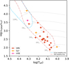 |
Fig. 2 HR diagram of our target stars with spectra in the blue region. The luminosity came from Gaia DR3 data bolometric corrected (see Sect. 5.3 for details). The effective temperatures were deduced with the SME package (see Sect. 5). The colors in the diagram represent the type of stellar variability. The instability strips calculated by Miglio et al. (2007) for β Cep and SPB stars are also shown. Some evolutionary tracks have been plotted to provide further information. The error bars in the diagram represent the uncertainties discussed in the text. |
5.2 Evolutionary trajectories
To determine the parameters of log (L/L⊙), M/M⊙, R/R⊙, and age presented in Table 2, we used the MESA code (Paxton et al. 2013, Modules for Experiments in Stellar Astrophysics, version r10398)4. This code allowed us to calculate the evolutionary trajectories of stars in the non-rotating regime. Our calculations were conducted with a burning shell overshooting prescription, where the overshooting parameter (fov) was set to 0.02, expressed in pressure scale heights. We considered a range of central hydrogen mass fraction variation between 0.001 to 1.0 from the zero-age main sequence, to terminal-age main sequence, and base metallicity (Z) of 0.02.
For the opacity tables and chemical mixtures, we relied on the standard data provided by MESA. Specifically, we used the OPAL Type 2 opacities developed by Iglesias & Rogers (1993) for the pre-main sequence and the Asplund et al. (2009) for the main sequence. Our calculations progressed with the initial hydrogen nucleus’s burning until the final helium nucleus was burned. This comprehensive process allowed us to determine the evolutionary trajectories of stars in the pre-main sequence, which served as the input parameters for calculating the main sequence trajectories.
The obtained trajectories represent the main sequence and are considered the outputs of our simulations. We generated a grid encompassing a range of stellar masses from 1.8 to 12 solar masses, spanning pre-sequence and main-sequence stages. The step size was 0.02 solar masses up to 4.0 solar masses, and a step size of 0.05 solar masses was used between 4.0 and 12 solar masses. We extracted the desired parameters by systematically scanning the grid and considering the effective temperature Teff and log g values previously determined. Cross-referencing these data with the grid, we obtained corresponding values for stellar luminosities, masses, radii, and ages. The uncertainties associated with those parameters were determined by using the same grid and the combinations of the upper and lower 1σ limits of Teff and log g. We have included the pre-main and main sequence inlist files in Appendix F for reproducibility purposes.
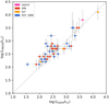 |
Fig. 3 Comparing the luminosities obtained from the MESA code, using our spectral observations, with those from the Gaia database. |
5.3 Luminosity distance
The luminosity obtained from our spectral observations using the MESA evolutionary code was compared in Fig. 3 with the one derived from the Gaia DR3 parallax (Gaia Collaboration 2016, 2023b). The comparison was performed following the documentation release 1.2 for Gaia’s Release 25. First, a geometric distance estimation was made using a Galaxy model by Bailer-Jones et al. (2018), which smoothly varies as a function of Galactic longitude and latitude. Bolometric corrections were then performed using tables provided by Bessell et al. (1998). As shown in Fig. 3, most of our luminosity determinations are consistent with Gaia’s within a 2 σ uncertainty.
We transformed the Gaia catalog’s extinction in the G filter to V magnitudes using the photometric relationship provided in the Gaia’s documentation aforementioned. Finally, the 1 σ error bars for the stellar parameters were calculated by considering the deviations from both parallax and bolometric correction.
5.4 Rotation and υ sin i
The projected surface rotation velocities for stars with blue spectra were estimated using a standard measurement procedure by means of the half-width at half-maximum (HWHM) of three photospheric lines: He I 4388 Å, He I 4471 Å and Mg II 4481 Å. The instrumental resolution was determined from the width of the calibration lines and quadratically subtracted from the υ sin i values in the spectra by a Gaussian fit. In some cases, the He I 4471 Å and Mg II 4481 Å lines were blended, making it difficult to measure the HWHM. If both He i lines were available, the average value was used. Otherwise, we took only the measurement for the He I 4471 Å line. If a measurement of the He I line was not possible, the Mg II measurement was used, corrected by a linear relationship obtained by comparing the υ sin i results from the He I 4471 Å and Mg II 4481 Å lines. In Sect. 7, a method is employed to estimate the average internal rotation frequency of some stars in the sample.
6 Probing inside the stars with g-modes
The presence of high-order (n ≫ ℓ) g-modes in chemically homogeneous, non-rotating stars with a convective core and a radiative envelope were predicted to be equally spaced in period through an asymptotic analysis (Tassoul 1980). The advent of high precision and long-duration space photometry has enabled the detection of consecutive g-modes in radial order with the same ℓ value and nearly equidistant spacings for γ Dor, SPB, and hybrid SPB/β Cep pulsators (Degroote et al. 2010, 2012; Pâpics et al. 2012).
The effects of rotation on the g-modes were rigorously calculated by Ballot et al. (2012). Rotation can substantially modify the stellar oscillation properties due to the centrifugal acceleration and the Coriolis force (see Bouabid et al. 2013). However, their results are valid only when the rotation rate is small relative to the mode frequencies and the Keplerian break-up rotation rate, which is often the case in SPB and γ Dor stars. Nevertheless, their results agree with the traditional approximation of rotation (TAR), introduced by Eckart & Gillis (1961) in geophysics and derived for stellar nonradial pulsations by Unno et al. (1989) and Lee & Saio (1997). The use of TAR simplifies the treatment of the pulsation equations even when the star’s rotation is considered. Under TAR, it has been shown that for a star with a convective core, the periods of low-degree, high-order g-modes have an asymptotic spacing (e.g., Basu & Chaplin 2017)
 (1)
(1)
where
 (2)
(2)
with N being the Brunt-Väisälä or buoyancy frequency and ℓ being the spherical degree of the pulsation. The limits of the radiative zone, where g-modes are trapped, are marked by r1 and r2. The characteristic time of gravity mode propagation within the star, often referred to as the buoyancy travel time (P0), is an essential factor in analyzing g-modes (Aerts 2021). Within the TAR, Ballot et al. (2012) demonstrated that for sufficiently high radial order pulsation numbers and in the presence of rotation, the asymptotic formula for the period spacing of g-modes could be written as follows:
 (3)
(3)
where m is the azimuthal order of a pulsation, s is the spin parameter, proportional to the ratio between the core’s angular rotation frequency and the angular pulsation frequency in the corotation frame (s = 2Ωcore/ωnℓm), and λℓ,m(s) represents the eigenvalues of the Laplace tidal equation in the longitudinal direction (as described in Unno et al. 1989). Also, λℓ,m(s) → ℓ(ℓ + 1) as s → 0, meaning that in the absence of rotation, the ΔPℓ formula is reduced to Eq. (1). It is worth noting that ΔPℓ decreases as ℓ increases. The typical ΔPℓ values for g-mode pulsations in SPB stars range between 5000 and 12 000 s (Aerts et al. 2019), which translates to P0 values between ~7000 and 17 000 s.
As high-order g-modes are observed to propagate deeply within main-sequence stars, the detected series of g-modes with the same degree (ℓ) and consecutive radial orders, along with their period-spacing patterns, provide a direct method to estimate the size of the star’s convective core (Degroote et al. 2010), the overshooting parameter and the mixing processes in the radiative region just above the core (Miglio et al. 2008; Aerts et al. 2010).
Aerts et al. (2018) proposed a robust, multi-step, iterative scheme to perform forward asteroseismic modeling of stars with convective cores based on observed gravity-mode oscillations of consecutive radial orders (n). Using the TAR framework, the authors analyzed high-precision Kepler data and, following the work of Van Reeth et al. (2016) and Ouazzani et al. (2017), made the assumption that the mode degree, azimuthal order, and the core rotation frequency (Ωcore) can be determined simultaneously from the rotational splitting or period spacing patterns. This method enables them to estimate the star’s mass, metallicity (X, Z), and core hydrogen content (Xcore) and to place constraints on the amount of convective core overshooting and the chemical mixing process in the radiative zone (see Aerts et al. 2018, and references therein for details).
The scheme also gives insight into the star’s evolution, as Xcore is a proxy for the age during the main sequence. Notably, the forward seismic modeling approach proposed by Aerts et al. (2018) is observationally driven, requiring unambiguous mode identifications in terms of spherical harmonic wavenumbers (ℓ, m) and observed frequencies that fit with theoretically predicted frequencies derived from stellar models. Furthermore, at a minimum, the seismic modeling method involves a five-dimensional (5D) optimization problem, as Ωcore must be estimated along with (M, X, Z, and Xcore). In recent years, a great number of SPB and γ Dor stars observed from space have been seismologically analyzed (e.g., Saio et al. 2021; Aerts 2021, and references therein).
7 Seismic diagnosis
Seismic analysis, as performed by Aerts et al. (2018), is beyond the scope of this paper. On the other hand, the expressions above for the period spacing (Eqs. (2) and (3)) are implicit because s depends on the pulsation frequencies. Then, the model-dependent and statistical methods proposed by Van Reeth et al. (2015), Christophe et al. (2018), and Li et al. (2019, 2020) to estimate Ωcore, P0 and the spherical harmonics wave numbers ℓ and m, employ multidimensional parameter spaces that result in cumbersome and time-consuming computations. Therefore, even estimating these parameters (as a first step in the seismic analysis of the stars) is not a straightforward task.
Fortunately, Takata et al. (2020) have come to our rescue. These authors have proposed a simplified, iterative method to perform mode identification and a simplified seismic diagnosis working in the frequency domain. The method uses the same simplifications mentioned above (asymptotic approach and TAR) and is only valid for prograde sectoral g-modes. Its application is relatively simple and efficient. They thus showed that for prograde g-modes (see details in their paper):
 (4)
(4)
(Takata et al. 2020, Eq. (11)) in which the factor fk(vrot) is written as:
![Mathematical equation: ${f_k}\left( {{v_{{\rm{rot}}}}} \right) = {\left[ {{{ - 1} \over {\left( {m{{\rm{\Delta }}_k}v} \right){{\rm{\Delta }}_k}}}\left( {{{\sqrt {{\lambda _{m,m}}(s)} } \over {{v_{{\rm{co}}}}}}} \right)} \right]^{{1 \over 2}}}\,\left( {{v_{k + {1 \over 2}}} - m{v_{{\rm{rot}}}}} \right),$](/articles/aa/full_html/2024/06/aa46439-23/aa46439-23-eq276.png) (5)
(5)
(Takata et al. 2020, Eq. (12)), where vrot is the average rotation frequency, k a counter and Δkν = vk+1 – vk is the difference between the (k + 1) and kth frequencies and  and vco = ν – mvrot. Bildsten et al. (1996) and Townsend (2003) showed that, for prograde sectoral modes, (ℓ = m > 0) and for s > 1,
  . Takata et al. (2020) validated their method by applying it to three γ Dor and one SPB star for which previous seismic analyses were done using Kepler data.
The iterative scheme of the method is as follows: (1) iteration 1: set fk to fk(1) = 1 and perform a least-squares fitting for Eq. (4) to estimate  and P0 = P0(1). (2) Iteration 2: calculate fk with
  into Eq. (5) and perform a least-squares fitting again for Eq. (4) to estimate
  and P0 = P0(2). (3) Iteration 3: repeat the same procedure as step 2 to estimate
  and P0 = P0(i+1) from the preceding
  (iteration i + 1) for i = 2, 3, … The process converges when both [
 ] and [
 ] are small enough.
As for other methods cited above that use the P – ΔP diagram, the Takata et al. (2020) method operates in the ν versus  plane and can only be applied to prograde sectoral g-modes of stars with a convective core surrounded by a radiative envelope, such as γ Dor and SPB stars, and allows for (a) mode identification performance, along with identifying prograde sectoral g-modes and distinguishing them from r (Rossby) and retrograde modes; (b) estimating the average rotation rate and the buoyancy travel time; (c) detecting the presence of buoyancy glitches in the stars.
The method given above is model-independent and based on a linear relationship between the oscillation frequency and successive square roots of frequency differences. As a matter of fact, Van Reeth et al. (2015) and Pâpics et al. (2017) showed that prograde sectoral modes are dominant in γ Dor and SPB stars and Li et al. (2019) reinforced this fact with a large sample of 611 γ Dor stars observed by Kepler. Indeed, 62% of the stars showed ℓ =1, m =1 (dipole) prograde modes. We expect many SPB stars to behave similarly and decided to check it by applying the simplified method to the stars in our sample. Aerts et al. (2019), in analyzing data issued from seismic analysis covering various stages of stellar evolution, showed that low- and intermediate-mass stars rotate quasi-rigidly during their core-hydrogen-burning phase. The average rotation rate estimated through Takata et al. (2020) method is thus a good estimation of For stars having prograde sectoral g-modes, the slope of the ν versus  line is the buoyancy travel time, P0, and the intercept is the average rotation frequency vrot. Last but not least, the wavy structure (signature of buoyancy glitches) appearing in the P-ΔP diagrams, caused by the presence of a chemical gradient near the stellar core (Miglio et al. 2008), is also seen in the ν versus
  diagram, although the method does not provide tools for exploring further this phenomenon.
For both SPB and γ Dor stars, frequency values are often grouped in more than one region, corresponding to the same ℓ but different m = 1, 2, 3… or corresponding to g and r modes (Kurtz et al. 2015; Saio et al. 2018). The frequency intensity decreases with increasing m (Van Reeth et al. 2016; Christophe et al. 2018; Saio et al. 2018; Takata et al. 2020). Moreover, the frequency groups can be easily distinguished by their different slopes in the ν versus  diagram. An important point to consider when applying Takata et al. (2020) method is that in the sequence of observed frequencies for a star, “jumps” in the radial order Δkn of 2, 3, 4,…units may occur. In the ν versus
  diagram, these points will be distant from the line corresponding to the n =1 frequencies by
  ,
,  ,
,  … (see Eq. (4)). The lines corresponding to these successive “jumps” have the same abscissa intercept as the baseline but a steeper slope by a factor
  with j = 2, 3, 4, … They can thus be interpreted as missing j–1 radial orders with Δkn = j (Takata et al. 2020). This method thus allows us to determine not only vrot and P0, but also Δkn.
7.1 Testing our frequency detection pipeline method
Christophe et al. (2018) analyzed nearly 670 days of Kepler data of the γ Dor star KIC 12066947 and identified 22 frequencies that were grouped in two clusters, around 22 μΗz and 32 μΗz. Takata et al. (2020) applied their method to the observed frequencies between 27 μΗz and 35 μΗz, which they had previously identified as prograde sectoral g-modes with m = 1. The results, shown in their Fig. 6, yielded an average rotation frequency of vrot = 24.88 ± 0.04 μΗz and a characteristic period of P0 = 4.08 ± 0.04 × 10³ s.
To verify the consistency of our results with previous studies, we applied our frequency detection pipeline to the same data of the γ Dor star KIC 12066947 obtained by Christophe et al. (2018). We obtained the same 22 frequencies within the acceptable errors and grouped them similarly to those reported by those authors. Furthermore, when using the method proposed by Takata et al. (2020) to analyze the frequencies within the range of 27 μΗz and 35 μΗz, we obtained results shown in Fig. 4, which are comparable to those presented in Fig. 6 of Takata et al. (2020). A linear regression analysis of our results yielded a rotation frequency of vrot = 24.8 ± 0.2 μΗz and P0 = 3.99 ± 0.05 × 10³ s, in agreement with the values of Takata et al. (2020). This further supports the consistency and validity of our methods and results.
7.2 Applying Takata’s method to the K2 shorter light curves
To further investigate the potential for using Takata et al.’s method to shorter observation spans, we applied it to the frequencies deduced from a 93.4 d light curve of KIC 12066947, observed during quarter ten only (compared to the almost 670 days of data used in the previous test). The results, shown in the diagram ν versus  in Fig. 5 were promising and yielded similar results to those obtained from the more extended data set, with a rotation frequency of vrot = 24.8 ± 0.3 μΗz and a buoyancy travel time of P0 = 4.0 ± 0.1 × 10³ s. Therefore, the regression line calculated with a much shorter data set, yields consistent results for the rotation frequency (vrot) and characteristic period of gravity modes (P0) as for the analysis of 670 days of data shown previously. However, it should be noted that the first two shorter frequencies appearing in Fig. 4 do not show up in the analysis of the shorter data set (from quarter 10, shown in Fig. 5). This suggests that while the results may still be reliable for shorter observation periods, they may be less accurate or less robust when using shorter data sets.
We applied the Takata et al. (2020) method to frequencies deduced for the SPB stars in our sample to try to estimate their average rotation rate, vrot and the buoyancy travel time, P0, for some of our stars. It should be remembered that the method only works for prograde g-modes and that Van Reeth et al. (2015) and Pâpics et al. (2017) showed that prograde sectoral modes are dominant in γ Dor and SPB stars. Indeed, Li et al. (2019) showed that 62% of 611 γ Dor stars observed by Kepler exhibited dipole prograde sectoral modes (i.e., with ℓ =1, m =1). As far as vrot value is concerned, it can range from very small for very slow rotators up to the Roche critical rotation frequency vcrit. This critical frequency depends on the stellar mass and radius (see below). For B0-B9 main-sequence stars,  . Table 3 shows the vrot and P0 values obtained for 14 B-type stars of Kepler Campaign 11 for which the method gave coherent results. The corresponding ν versus
  diagrams can be seen in Figs. E.1–E.6, where the frequencies corresponding to different radial orders are shown in different colors.
The B stars in Table 3 have luminosity classes from I to V. Giant stars have larger radii, but their internal structure is similar to main-sequence stars, in the sense that they also have a convective core surrounded by a radiative envelope (Langer et al. 2010; Kippenhahn et al. 2012).
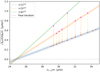 |
Fig. 4 ν versus |


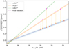 |
Fig. 5 ν versus |

Average rotation frequencies and buoyancy travel times for 14 B stars of Kepler/K2 campaign 11 estimated, using the method from Takata et al. (2020).
8 Correlations between spectroscopic and seismic parameters
Correlations between spectroscopic and seismic parameters were predicted by theory and have been confirmed during the last decade.
8.1 Nonradial pulsation excitation and the dependence of pulsation periods on stellar temperature
Theoretical calculations by Dziembowski et al. (1993) and Dziembowski (1998) indicate that the κ mechanism in the metal-bump zone at T ≈ 2 × 10⁵ K is responsible for nonradial pulsation excitation across the main sequence, from late B to O spectral types. In the SPB region, high-order g-modes, particularly the strong dipole (ℓ = 1) and quadrupole (ℓ = 2) modes, with frequencies ranging from around 0.3–5 day−1 are unstable (Pedersen et al. 2021a). The κ mechanism suggests that pulsation modes in stars are only excited if their periods are comparable to or longer than the thermal timescale in the Z-bump zone. In SPB stars, this timescale is approximately 2.5 times greater than that for β Cep stars, which is compatible with the observed pulsation periods. The longer thermal timescale in the Z-bump zone of SPB stars leads to a preference for the excitation of higher period modes. Additionally, Fig. 8 of Dziembowski et al. (1993) shows that hotter stars have shorter pulsation periods for each SPB stellar-mass interval. As the timescale of the Z-bump zone decreases with increasing Teff, this implies that the dominant frequency should also increase with temperature (e.g. Pamyatnykh 1998, Fig. 1; Pamyatnykh 1999, Fig. 2).
8.2 Observed multivariate correlations between spectroscopic and seismic parameters
The study of γ Dor and SPB stars exhibiting g-mode pulsations has led to the discovery of multivariate relationships between physical and seismic parameters (De Cat & Aerts 2002; Bouabid et al. 2013; Aerts et al. 2014; Van Reeth et al. 2015; Pâpics et al. 2017, and references in these papers). For example, Aerts et al. (2014) observed a significant correlation between Teff and the dominant frequency fg of g-modes in a sample of 68 OB stars, with the coolest stars exhibiting higher observed dominant frequencies than hotter stars (their Fig. 2). We found a similar trend in our sample of 45 SPB stars. However, this observed temperature-frequency dependence does not agree with theoretical predictions (see above). To further discuss this question with its untangling with the stellar rotation is beyond the scope of this paper.
Van Reeth et al. (2015) studied correlations between physical and seismic parameters for a sample of 41 γ Dor stars that showed prograde sectoral g-modes and were observed by the Kepler spacecraft. The researchers employed multivariate analyses to examine the relationships between various stellar parameters obtained from spectroscopy and pulsation parameters. Their analysis revealed a strong correlation between the longest detected pulsation period PMax of the downward pulsation pattern and the stellar rotation (measured through ν sin i) (their Figs. 9 and 10) and a weaker correlation between the frequency of the dominant g-mode fg and ν sin i. Furthermore, they note that PMax can be considered indicative of the cutoff frequency at which radiative damping of the pulsations becomes dominant over the excitation mechanism. Therefore, PMax provides information on the physical conditions governing the existence of unstable g-modes and the boundaries of the instability strip (Dupret et al. 2005; Bouabid et al. 2013; Van Reeth et al. 2015; Pâpics et al. 2017, and references therein). For the γ Dor stars, the researchers found the expected correlation between Teff and fg, with the dominant frequency increasing with temperature. They attributed the difference in trend between Teff and fg for γ Dor and SPB stars to the difference in the extent of the instability strip of the two types of stars. The main physical parameter contributing to the trend for the former group is the stellar radius, while it is the initial mass for the latter group.
Values of PMax and the frequency of the dominant mode are significantly influenced by rotation. A faster rotation of the star causes greater shifts in pulsation frequencies, resulting in a period spacing pattern with a steeper downward slope and more closed spacing. As a result, prograde modes have shorter pulsating periods. However, Bouabid et al. (2013) demonstrated that the upper limit of unstable modes for prograde sectoral modes increases with rotation for γ Dor stars, while the number of unstable modes decreases. Conversely, non-prograde sectoral modes display the opposite trend, resulting from the competition between driving at the base of the convective envelope and damping in the g-mode cavity. Finally, it is worth noting that Van Reeth et al. (2015) found a trend opposite to the one predicted by Bouabid et al. (2013).
Our analysis of Kepler/K2 SPB data from Campaign 11 has thus revealed a correlation between astrophysical and seismic parameters for our stars, specifically between the dominant g-mode frequency (fg) and υ sin i. Our correlation agree with that found by Aerts et al. (2014). In order to better understand this correlation and eliminate the effect of the inclination angle as a physical parameter, we examined the relationship between (fg) and the average internal rotation estimated using Takata’s method for some of our stars (see Sect. 7). To improve our sample, we included SPB stars from Kepler data analyzed seismically by Pedersen (2022, priv. comm.), who determined the average internal rotation velocity by modeling the dipole period spacing patterns. Our results are shown in Fig. 6, which indicate an increase in (fg) with increasing rotation rate. However, the correlation has a considerable dispersion, suggesting that other physical parameters are contributing to the observed trend.
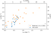 |
Fig. 6 Relationship between the dominant frequency of g-modes fg and the average internal rotation frequency for SPB stars. Blue points represent values deduced using the Takata et al. (2020) method (this work), while orange points are values estimated by Pedersen et al. (2021a) from modeling the dipole period spacing patterns, in a data set from original Kepler mission. Error bars are generally smaller than the plot symbols. The observed trend indicates an increase in the dominant frequency of g-modes with the internal rotation frequency, although the loose correlation suggests that other physical factors are also at play. |
8.3 Determining stellar rotation frequencies limits
We can verify whether the average rotation frequencies estimated using the technique outlined in Takata et al. (2020) are compatible with the Roche critical rotation frequency. Zorec et al. (2016) described this critical frequency as:

Alternatively, we can establish a minimum value for the rotational frequency using the equatorial velocity calculated for an inclination angle of sin i = 90°. This value can be obtained as follows:

with the frequency  in d−1, in km s−1, and R in R⊙ (Balona et al. 2019). In this expression, veq = υ sin i for i = 90°.
The stellar rotation frequency’s upper and lower limits depend on the star’s mass and radius. To determine these limits for the fourteen stars in our sample, we used evolutionary data from Straizys & Kuriliene (1981) and data for main sequence stars measured in binary systems (Torres et al. 2010). Using the Takata et al. (2020) method, we estimated each star’s average internal rotation frequency, which are given in Table 3. In all cases, these frequencies happen to lie between the critical and minimal frequency values.
9 Summary and conclusions
We analyzed the light curves of 122 B-type star candidates observed during quarter 11 of the Kepler/K2 mission campaign. Variability types were determined through frequency analysis, light curve characteristics, spectroscopic observations, comparisons to previous observations, and contextual information. For each star, the frequency with the largest amplitude and the total number of frequencies detected are indicated, including harmonics and frequency combinations. We classified the variability types following criteria proposed by Balona et al. (2011), McNamara et al. (2012), and Bowman et al. (2019a). Our results show that 41 stars are SPB stars. For 53 objects, the primary variability was attributed to binarity, rotation, or both. We also identified five stars showing Maia/fast-rotating SPB variables, with two classified as hybrid SPB/β Cep pulsators and one as a β Cep binary. Thirteen stars in our sample exhibit a dominant, low-frequency power excess, indicative of SLF variability. In addition, we pointed out six objects of interest that warrant further investigation.
We also present an analysis of a subset of 45 B stars out of the 122 B star candidates observed in Kepler/K2 Campaign 11. Their mid-resolution spectra were obtained in the blue region at OPD/LNA, Brazil. Physical parameters such as spectral classification, projected rotation velocities υ sin i, and luminosity values were determined using SME and MESA algorithms. A classical stellar classification based on the appearance of the wings of the Balmer lines and on He I, O II, Si III, and Mg II line ratios were also applied to the spectra. Our spectroscopic analysis showed that the luminosity values obtained are compatible with the photometric results obtained with Gaia data. Combining the frequency analysis, variability classification, and seismic analysis of these stars provided consistent results. Using the ν versus  Takata et al. (2020) method, we estimated the average internal rotation frequency and the buoyancy travel time for 14 stars in our sample. Two of these stars were classified as SPB + Maia variables. They showed high internal rotation frequencies, which agree with the conclusion by Balona (2023) that Maia variables do not rotate faster than SPB stars, on average. The fact that applying the method to these stars with coherent results suggests that these hybrid stars exhibit sectoral dipole nonradial pulsations. Further investigations of these stars could provide insights into the type of mechanism driving their pulsations.
Many authors found multivariate relationships between physical (e.g. Teff and υ sin i) and seismic (e.g. the dominant frequency, fg, and the maximum observed period, PMax) parameters for γ Dor and SPB stars. To improve this analysis and eliminate the unknown inclination angle, we used the internal rotation frequency estimated in this paper as one of the variables. Our analysis revealed a positive correlation between the dominant frequency fg and the internal rotation frequency, vrot, for our sample of B stars, which was extended with the data of Pedersen et al. (2021b) obtained from Kepler observations. They deduced the internal rotation from modeling the dipole period spacing patterns. Specifically, we found that the dominant frequency increases with increasing rotation frequency. However, the high correlation dispersion suggests that other factors contribute to the relationship.
Furthermore, SPB stars and β Cephei stars are types of B stars characterized by nonradial pulsations. SPB stars pulsate in g-modes, while β Cephei stars pulsate in p-modes. Both types of pulsations are believed to be driven by the κ mechanism. Current models involving deep internal core pulsations of B stars have limitations and other factors, such as convection and the presence of starspots, may play a role in the driving of pulsation mechanisms. Therefore, a more complex scenario may be necessary to explain the pulsation behavior of B stars, with different roles for each type of star. In addition, further studies using spatial-frequency precision and high-resolution spectroscopy will be decisive in enabling detailed asteroseismic analyses. These studies could provide a better understanding of the long-term variability behavior, structure, and evolution of these stars.
Acknowledgements
We thank Dr. May G. Pedersen for kindly providing us with her data on internal rotation of SPB stars observed with the Kepler satellite. This study was financed in part by the Coordenaçâo de Aperfeiçoa-mento de Pessoal de Nivel Superior - Brazil (CAPES) - Finance Code 001, by Fundaçâo de Amparo à Pesquisa do Estado de Sâo Paulo (FAPESP) through grant 2016/13750-6, and by the State of Parana Secretary of Science, Technology and Higher Education - Fundo Parana. This research was partly supported by NASA Contract NAS5-02139 to Stanford University. M.E. gratefully acknowledges the financial support of the “Fenômenos Extremos do Universo” of the Fundaçâo Araucaria. This paper includes data collected by the Kepler mission and obtained from the MAST data archive at the Space Telescope Science Institute (STScI). Funding for the Kepler mission is provided by the NASA Science Mission Directorate. STScI is operated by the Association of Universities for Research in Astronomy, Inc., under NASA contract NAS 5-26555. This work has made use of data from the European Space Agency (ESA) mission Gaia (https://www.cosmos.esa.int/gaia), processed by the Gaia Data Processing and Analysis Consortium (DPAC, https://www.cosmos.esa.int/web/gaia/dpac/consortium). Funding for the DPAC has been provided by national institutions, in particular the institutions participating in the Gaia Multilateral Agreement. This work made use of the https://Gaia-kepler.fun crossmatch database created by Megan Bedell. All light curves analyzed in this work were retrieved from public K2 data hosted on the Mikulski Archive for Space Telescopes (MAST) Portal at https://archive.stsci.edu/. Spectroscopic data underlying this article are available in the article and in its online supplementary material. This paper is also based on observations obtained at the Pico dos Dias Observatory/LNA/MCTI. This work has made use of the VALD database, operated at Uppsala University, the Institute of Astronomy RAS in Moscow, and the University of Vienna.
Appendix A Table featuring classifications for all targets
We summarize the variability characteristics of the stars in our sample in the table below. The variability class symbols are SPB for Slowly Pulsating B-type stars; HYB for stars with both β Cep and SPB frequencies; MAIA for stars belonging to the MAIA group of variables (Balona & Ozuyar 2020) or fast-rotating SPB stars; ROT for stars with rotation effect present; EBIN for eclipsing binary; SLF for Stochastic Low-Frequency variability. We refer to Section 4 for more details. We report the number of detected frequencies and the highest-amplitude frequency for pulsating targets. In the last column, we use the following symbols: “n Fg” for n frequency groups, “ELL” for ellipsoidal-type variation (non-eclipsing close binary systems with gravitationally distorted components and additional reflection and beaming periodicity, see Morris 1985), and “spots” for light curve with spot signatures.
Program stars and their main variability characteristics.
Appendix B Especially interesting stars
We highlight below a selection of stars from our sample that are of particular interest and merit further study. They occupy the upper part of the Gaia HR diagram. (see Table A.1 for a complete listing by EPIC number).
EPIC 223160833 (CD −26 12352/ALS 4393) is a V = 10.20 eclipsing binary with a primary star classified as a β Cep. Before our analysis, information about this binary was scarce in the literature it being simply listed in catalogs. The SIMBAD database classifies the star as “OB,” a type of classification first introduced by Slettebak & Stock (1957) based on spectra taken with photographic plates. They also concluded that the majority of OBstars out of 61 objects, occurred for luminosity classes III and V. However, a few supergiants (class Ib) and luminous giants (class II) were also observed. The presence of β Cep stars in binary systems is rather rare. Indeed, the first two high-precision measurements of masses and radii of β Cep stars were performed only recently (Southworth et al. 2020; 2021). EPIC 223160833 is thus a β Cep eclipsing binary that deserves further study. It occupies a position in the Gaia HR diagram in the region of β Cep stars. The K2 light curve (Fig. B.1, upper panel) is typical of an eclipsing binary with unequal depths, with an orbital period of approximately ~4.9 d. The frequency spectrum (Fig. B.1, middle panel) shows frequencies characteristic of both β Cep and SPB stars, and we classified this object as a hybrid star. It’s possible that the main component of this system is a non-hybrid β Cep, given that most of the frequencies below 5 day−1 are due to the eclipses, and pulsations can also be seen in the fainter partner. The Balmer lines are generally well marked in this class of stars, but the He I lines are weak. However, as shown in our spectrum of this object in Fig. B.1, lower panel, the He I lines are rather conspicuous.
Despite it being an eclipsing binary, the blue spectrum of the star and the results of our SME/MESA analysis are consistent with a B2 III object located in the β Cep instability strip in the HR diagram (see Fig. 1). Additional observations of this binary star will determine its components’ mass and radii precisely and could add a deeper understanding of the internal rotation and mixing of the primary. Those observations will help to shed light on the evolutionary status of the system and provide insight into the physical processes that drive the variability.
EPIC 223207465 (HD 161610) is a V = 9.07 star classified as B5 II in the SIMBAD database. Our spectrum analysis supports this classification (see Fig. B.2, lower panel). However, the line ratios in the spectrum do not provide enough information to differentiate between luminosity classes III and IV. Our SME/MES A analysis of the spectrum indicates that this object has left the Main Sequence and shows the following physical parameters:  ,
,  ,
,  ,
,  and
and  . The light curve, shown in Fig. B.2, upper panel, suggests the presence of a rotation modulation with period ~3.5 d. Bowman et al. (2019b) have reported the detection of SLF frequencies in this object, also seen in our K2 frequency spectrum, as shown in Fig. B.2, middle panel. Based on these observations, we classify this star as a B5 III ROT. It is thus a typical early SPB star showing also the SLF phenomenon. Through a simplified seismic diagnostics, we concluded that this star rotates with an average frequency of 4.3 μHz (~0.37 day−1 ) and a characteristic period of gravity modes (also called the buoyancy travel time) P0 = 4.3 · 103 s. A more detailed asteroseismic analysis of this object would be important to gain a deeper understanding of the properties and behavior of this kind of giant star.
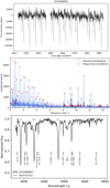 |
Fig. B.1 Light curve, frequency spectrum, and blue spectrum of the binary star EPIC 223160833 (ALS 4393) whose primary is a β Cep variable. The K2 light curve in the upper panel is characteristic of an eclipsing binary with an orbital period of ~4.9 d. The middle panel displays the frequency spectrum, which shows frequencies typical of both β Cep and SPB variables. The star is thus classified as a hybrid. The frequency corresponding to the binary period is marked with a red dot, at ~0.2 day−1. The lower panel shows the blue spectrum of the star, with prominent Balmer and He He I lines which is consistent with a B2 III spectral classification. The lines of the companion of this bright β Cep star are not visible. |
EPIC 223217668 (IGRJ 17541–2619) is an X-ray source discovered by the INTEGRAL and RXTE high-energy satellites in the inner arms of the galaxy, as reported by Pellizza et al. (2006, and references therein). It is a heavily reddened highmass X-ray binary with an O9 Ib primary and a neutron star companion, where the primary dominates the visible-IR flux. It is thus a bright star and is the reddest one in our sample. The light curve, as shown in the upper panel of Fig. B.3, is typical of a hot, supergiant object that exhibits apparently erratic variations. We detected low frequencies in this star which we interpret as stochastic SLF-type variability and frequencies typical of gmodes currently observed in SPB (see Fig. B.3, lower panel). Stochastic variability is often found in massive X-ray sources, as noted by Bult (2017). This star was classified by us as SPB + SLF (see Table A.1). As for the previous star, a simplified seismic diagnostics applied to EPIC 223217668 estimates that the star rotates with an average frequency of 4.3 μHz (~0.37 day−1 ) and has a characteristic period of gravity modes (buoyancy travel time) P0 = 13.4 · 103 s. A deeper seismic analysis would be important in this case to further understand the presence and consequences of stochastic low-frequencies in a late O supergiant star.
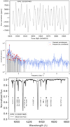 |
Fig. B.2 Same details as in Fig. B.1, but for EPIC 223207465 (HD 161610), which is classified as a B5II star in the Simbad database. The K2 light curve in the upper panel exhibits a periodicity of approximately 3.5 d, probably due to a rotation modulation effect. Indeed, the frequency spectrum in the middle panel shows a prominent peak at frequency 0.28 day−1, corresponding to this period, in addition to many low-frequency periodicities, consistent with the SLF phenomenon, as noted by Bowman et al. (2019b). Lower panel: Star’s blue spectrum, which confirms a B5II-III classification (see text). |
EPIC 230819479 (BD –18 4436/LSE 3/IRAS 17074-1845) is a hot, “post-AGB proto-planetary nebula” (PEAGB or PPN) (Parthasarathy et al. 2000). Such objects are intermediate-mass stars in the fast transition between the late asymptotic giant branch (AGB) phase and the subsequent planetary nebula (PN) phase, which typically lasts for a thousand years. These post-early AGB (PEAGB) stars leave the AGB, cross the HR diagram, and descend the WD cooling curve (e.g., Kastner 2005; Brown et al. 2008; Kippenhahn et al. 2012). Since their late stages in the AGB, the star undergoes violent structural changes and mass ejection episodes, usually showing many absorption and emission lines, both permitted and forbidden, and P-Cyg profiles in Balmer lines, typical of a substantial mass loss (e.g., Arkhipova et al.). The position of EPIC 230819479 in the Gaia HR diagram is compatible with a bright star of about 6 M⊙, having already left the main-sequence. Its K2 light curve shows semi-regular variability, with one strong outburst lasting ~eq6.5 d (at about BJD 2860, see Fig. B.4, upper panel). The power spectrum shows a bunch of frequencies typical of SLF and a few frequencies characteristic of SPB stars. The star has been fainter by about two mags since the 1950’s. (Arkhipova et al. 2014), and its IR colors are typical of hot post-AGB stars. Understanding these stars’ variability patterns and trends could help refine their theoretical evolutionary tracks (Carmona et al. 2010). Carmona et al. (2010) made a detailed spectral analysis of this star from FEROS high-resolution (R ~eq 45 000) rich line spectrum and classified it as a B5 Ibe object. Mello et al. (2012) made an abundance analysis using the same instrument and estimated a spectral type of B3 IIIe, but their log g value of 2.05 is more typical of a luminous supergiant star and its position in Gaia HR diagram is compatible with a bright star of about 5 M⊙, having already left the main-sequence. Its IR colors are typical of hot post-AGB stars (Parthasarathy et al. 2000). We thus adopt for this star the Carmona et al. (2010)’s spectral classification of B5 Ib e. Understanding the variability patterns and trends of PEAGB stars would help to refine their theoretical evolutionary tracks.
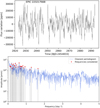 |
Fig. B.3 K2 light curve of the O9 Ib X-ray binary EPIC 223217668 (IGRJ 17541–2619), which displays erratic variations typical of a hot, supergiant object, shown in the upper panel. The lower panel depicts the frequency spectrum, displaying both SLF and SPB frequencies. It could be interesting to further analyze the presence and impact of SLF variations in a late O supergiant X-ray binary. |
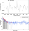 |
Fig. B.4 K2 light curve of EPIC 230819479 (BD–184436), a post-AGB/PPN star, shown in the upper panel. An outburst seems to occur near BJD 2860, and the star shows variations in a timescale of ~ days, as reported by Henson & Deskins (2009). Lower panel shows the star’s frequency spectrum which shows an intense concentration of low-frequencies characteristic of the SLF phenomenon plus several frequencies in the SPB region. |
EPIC 231153467 (CD–24 13065) is also a post-AGB/proto-PN (PPN) star, as discovered by Schiavon et al. (2012). The same general comments concerning PEAGBs apply here. However, the two light curves are rather different. EPIC 231153467 has a standard, sinusoidal light curve (see Fig. B.5, upper panel), with an apparent periodicity of ~6 d. It also shows two more outstanding frequencies at ~10.3 day−1 and ~1.1 day−1 perceived on top of the more prolonged modulation. The power spectrum shows frequencies typical of the SLF phenomenon and some that could be attributed to SPB variables, plus many periodicities above 5 day−1, typical of β Cep stars (Fig. B.5, middle panel). The SME/MESA analysis of our blue spectrum (Fig. B.5, lower panel) yields  , log
, log  ,
,  ,
,  and
and  . Based on the Balmer and line ratios, these physical parameters are compatible with our B3 III classification. The star is a PEAGB younger than the previous EPIC 230819479 (BD–18 4436), as suggested by the form of the light curve and the lack of emission in the Balmer lines (Suárez et al. 2006). Again, it is essential to study PEAGB stars to better understand their evolutionary tracks.
EPIC 240255386 (CD–29 13906) is classified as a B0 Ia star in the SIMBAD database. This star is also an X-ray source detected by XMM and Chandra satellites (Nazé 2009; Rauw et al. 2015). The log LX/ log Lbol ratio is typical of single O stars, which means that the X-rays are probably produced by shocks in the radiatively driven wind Rauw et al. (2015). The light curve is characteristic of a hot, luminous object, as seen in the upper panel of Fig. B.6. The frequency spectrum displays mainly low-frequency periodicities (SLF) and a few ones in the SPB region, which is compatible with the B0 Ia classification (Fig. B.6, lower panel). A deeper asteroseismic analysis would be important to better understand this single luminous B0 star.
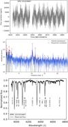 |
Fig. B.5 K2 light curve of EPIC 231153467 (CD-24 13065), another post-AGB/PPN star, shown in the upper panel. Note the apparent periodicity of ~6 d. The star’s frequency spectrum, is shown in the middle panel, exhibiting frequencies characteristic of the SLF phenomenon plus some that could be attributed to SPB variables and many frequencies above 5 day−1, typical of Beta Cephei stars. Blue spectrum of the star obtained in Brazil, which is consistent with a B3 III classification, shown in the bottom panel. The absence of emission in the Balmer lines suggests that the star is likely a young post-AGB star. |
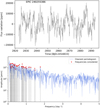 |
Fig. B.6 K2 light curve of EPIC 240255386 (CD–2913906/J 174350.9–295911), shown in the upper panel, displays the typical variability of a hot, luminous star. The lower panel displays its frequency spectrum, showing frequencies both in the SLF and SPB regions, as expected for a B0 Ia star, quoted in the Simbad database. |
Appendix C Light curves and frequency spectra
The upper panel displays the light curves of the star, with its EPIC identifier6. The middle panel shows the wavelet transform of the light curves. The lower panel presents the frequency spectra of the stars, with the blue line indicating the frequencies obtained using the CLEANEST method and triangles indicating the frequencies found with the IVS-KULeuven iterative prewhitening routine (Degroote et al. 2009). Each star is identified by its EPIC number.
Appendix D Spectra
This plot contains the blue spectra of 45 stars obtained at Pico dos Dias Observatory (black line)7. Main lines are signaled. Red lines represent the spectral model from SME with the parameters shown in Table 2. In some cases the normalization procedure ended up distorting the Hδ region. For these cases, the region was masked out of the model and denoted by a dotted line.
Appendix E ν versus  diagrams and results
In this appendix, we present the obtained diagrams with the application of Takata et al. (2020) method, for the stars present in Table 3. The following paragraphs highlight some results.
EPIC 221788083 (HD 316214) is a SPB + SLF B8 star with 57 detected frequencies, 11 of which correspond to ℓ =1, m =1. The ν versus  diagram reveals vrot = 6.1 ± 0.1 μHz, P0 = 4.9 ± 0.2 · 103 s (Fig. E.1).
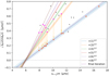 |
Fig. E.1 ν versus |


EPIC 223217668 (IGRJ 17544–2619) is a SPB + SLF O9 Ib X-ray binary star with 25 detected frequencies, seven corresponding to ℓ = 1, m = 1 seismic pulsations. The ν versus  reveals vrot = 4.3 ± 0.2 μHz, P0 = 13 ± 1 · 103 s (Fig. E.2). This quite large P0 value is consistent with the star being a supergiant O9Ib.
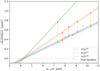 |
Fig. E.2 Same details as in Fig. E.1, but for EPIC 223217668. The diagram shows frequencies between 7.0 and 10.8 μHz attributed to prograde sectoral modes with m =1. The results obtained are: vrot = 4.3 ± 0.2 μHz, P0 = 13 ± 1 · 103. |
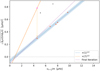 |
Fig. E.3 Same details as in Fig. E.1, but for EPIC 227807830. The diagram shows frequencies between 4.2 and 11.0 μHz attributed to pro-grade sectoral modes with m = 1. The results are: vrot = 1.1 ± 0.2 μHz, P0 = 8 ± 1 · 103. |
EPIC 227807830 (HD 158661) is a SLF B0II star with 18 detected frequencies, six corresponding to ℓ = 1, m = 1 seismic pulsations. Through the ν versus  diagram analyses we found vrot = 1.1 ± 0.2 μHz, P0 = 8 ± 1 · 103 s (Fig. E.3). The low rotation frequency confirms the results of Jönsson et al. (2020) that report for the star v sin i = 3.3 km s−1.
EPIC 231532027 (HD 155311) is a SPB B7II-III star with 64 detected frequencies, 12 corresponding to ℓ =1, m =1 pulsations. Our spectral analyses yields  ,
,  ,
,  ,
,  ,
,  , v sin i = 100 ± 25, and age
  and the B7 II-III spectral classification. The ν versus
  diagram indicates vrot = 6.2 ± 0.1 μHz, P0 = 4.4 ± 0.2 · 103 s (Fig. E.4).
EPIC 235178852 (CD-23 13201) is a faint (V = 12.6) blue star classified simply as “OB +” in the SIMBAD database. We detected in this star 46 SLF + SPB frequencies, 13 of which corresponding to ℓ = 1, m = 1 pulsations. Takata et al’s method applied to this star yields vrot = 4.5 ± 0.1 μHz, P0 = 11.3 ± 0.3 · 103 s. The light curve is typical of a highly variable supergiant star. Its position in the Gaia HRD (Fig. 1, Paper I) indicates that this is a rather luminous object, situated near the 8 M⊙ evolutionary track. We thus estimate for this star a spectral classification B II-I, in accordance with its great P0 = 11.3 value (Table 3).
EPIC 238194885 (HD 158195) is a SPB + SLF B2III star with 31 detected frequencies, 9 of which correspond to ℓ = 1, m = 1 pulsations. The ν versus  diagram yields vrot = 7.0 ± 0.3 μHz, P0 = 6.4 ± 0.5 · 103 s (Fig. E.5).
EPIC 240255386 (CD–29 13906) is a SPB + SLF B0Ia X-ray source with 39 detected frequencies, 9 corresponding to ℓ =1, m =1 pulsations. Applying Takata et al.’s method yields for this star vrot = 6.0 ± 0.1 μHz, P0 = 7.1 ± 0.3 · 103 s (Fig. E.6).
There are two stars classified as SPB + Maia variables (EPIC 240276653 and 242049665) in Table 3. It is quite interesting to verify what results we get for these stars in terms of the seismic parameters vrot and P0. It can be seen that they show two of the highest vrot values in the table, but that there are other SPB variables that rotate relatively fast as well. These results are compatible with the conclusions of Balona (2023), that the two groups of Maia and SPB stars show on the average similar rotation velocities. Figures E.7 to E.14 show the remaining ν versus  diagrams from stars in table 3.
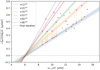 |
Fig. E.4 Same details as in Fig. E.1, but for EPIC 231532027, using frequencies between 8.5 and 15.0 μHz attributed to prograde sectoral modes with m =1. The results indicate a rotation frequency of vrot = 6.2 ± 0.1 μHz and a characteristic period of P0 = 4.4 ± 0.2 · 103 s. |
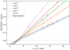 |
Fig. E.5 Same details as in Fig. E.1, but for EPIC 238194885, based on the frequencies used (8.7 and 13.7 μHz) attributed to prograde sectoral modes with m = 1. For this star, the results are: vrot = 7.0 ± 0.3 μHz, P0 = 6.4 ± 0.5 · 103 s. |
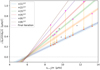 |
Fig. E.6 Same details as in Fig. E.1, but for EPIC 240255386. Frequencies between 8.4 and 13.7 μΗz were used, attributed to prograde sectoral modes with m =1. For this star, we find vrot = 6.0 ± 0.1 μHz, P0 = 7.1 ± 0.3 · 103 s. |
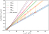 |
Fig. E.7 ν versus |

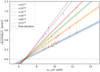 |
Fig. E.8 ν versus |

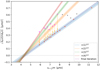 |
Fig. E.9 ν versus |

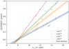 |
Fig. E.10 ν versus |

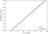 |
Fig. E.11 ν versus |

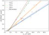 |
Fig. E.12 ν versus |

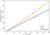 |
Fig. E.13 ν versus |

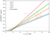 |
Fig. E.14 ν versus |

Appendix F Mesa files
inlist load
&star_job
    ! start a run from a saved model
      load_saved_model = .false.
      saved_model_name = ’1.8M_at_ZAMS.mod’
    ! display on-screen plots
      pgstar_flag = .true.
/ !end of star_job namelist
&controls
    ! use C/O enhanced opacities
    ! important for He-burning onwards
      use_Type2_opacities = .true.
      Zbase = 0.02
    ! configure mass loss on RGB & AGB
      cool_wind_RGB_scheme = ’Dutch’
      cool_wind_AGB_scheme = ’Dutch’
      RGB_to_AGB_wind_switch = 1d-4
      Dutch_scaling_factor =0.8
/ ! end of controls namelist
    inlist project - pre main sequence
! inlist to evolve a 2.0 solar mass star
! For the sake of future readers of this file (yourself included),
! ONLY include the controls you are actually using.  DO NOT include
! all of the other controls that simply have their default values.
&star_job
    ! begin with a pre-main sequence model
      create_pre_main_sequence_model = .true.
    ! save a model at the end of the run
      save_model_when_terminate = .true.
      save_model_filename = ’2.0M_at_ZAMS.mod’
    ! display on-screen plots
      pgstar_flag = .true.
/ !end of star_job namelist
&controls
    ! starting specifications
      initial_mass = 2.00 ! in Msun units
    ! stop when the star nears ZAMS (Lnuc/L > 0.99)
      Lnuc_div_L_zams_limit = 0.99d0
      stop_near_zams = .true.
    ! stop when the center mass fraction of h1 drops below this limit
      xa_central_lower_limit_species(1) = ’hi’
      xa_central_lower_limit(1) = 1d-3
/ ! end of controls namelist
    inlist project - main sequence
! For the sake of future readers of this file (yourself included),
! ONLY include the controls you are actually using.  DO NOT include
! all of the other controls that simply have their default values.
&star_job
    ! begin with a pre-main sequence model
      create_pre_main_sequence_model = .false.
    mesa_dir = ’../../../mesa-r10398’
    load_saved_model = .true.
    saved_model_name = ’2.0M_at_ZAMS.mod’
    ! save a model at the end of the run
      save_model_when_terminate = .true.
      save_model_filename = ’2.0M_final.mod’
    ! display on-screen plots
      pgstar_flag = .true.
/ !end of star_job namelist
&controls
    ! this stopping condition should get triggered
    log_L_upper_limit = 3.6
    ! this stopping condition should not get triggered
    Teff_lower_limit = 4700
    ! starting specifications
    ! initial_mass =4.94 ! in Msun units
    ! stop when the star nears ZAMS (Lnuc/L > 0.99)
    ! Lnuc_div_L_zams_limit = 0.99d0
    ! stop_near_zams = .true.
    ! stop when the center mass fraction of h1 drops below this limit
    ! xa_central_lower_limit_species(1) = ’hi’
    ! xa_central_lower_limit(1) = 1d-3
/ ! end of controls namelist
References
- Aerts, C. 2021, Rev. Mod. Phys., 93, 015001 [Google Scholar]
- Aerts, C., Christensen-Dalsgaard, J., & Kurtz, D. W. 2010, Asteroseismology (Springer) [Google Scholar]
- Aerts, C., Molenberghs, G., Kenward, M. G., & Neiner, C. 2014, ApJ, 781, 88 [Google Scholar]
- Aerts, C., Molenberghs, G., Michielsen, M., et al. 2018, ApJS, 237, 15 [Google Scholar]
- Aerts, C., Mathis, S., & Rogers, T. M. 2019, ARA&A, 57, 35 [Google Scholar]
- Aigrain, S., Parviainen, H., & Pope, B. J. S. 2016, MNRAS, 459, 2408 [NASA ADS] [Google Scholar]
- Alexeev, B. V. 2017, in Nonlocal Astrophysics (Elsevier), 321 [CrossRef] [Google Scholar]
- Amôres, Ε. B., Jesus, R. M., Moitinho, A., et al. 2021, MNRAS, 508, 1788 [CrossRef] [Google Scholar]
- Arkhipova, V. P., Burlak, M. A., Esipov, V. F., et al. 2014, Astron. Lett., 40, 485 [NASA ADS] [CrossRef] [Google Scholar]
- Arkhipova, V. P., Parthasarathy, M., Ikonnikova, N. P., et al. 2018, MNRAS, 481, 3935 [NASA ADS] [CrossRef] [Google Scholar]
- Asplund, M., Grevesse, N., Sauval, A. J., & Scott, P. 2009, ARA&A, 47, 481 [NASA ADS] [CrossRef] [Google Scholar]
- Avni, Y., & Bahcall, N. A. 1976, ApJ, 209, 16 [CrossRef] [Google Scholar]
- Bailer-Jones, C. A. L., Rybizki, J., Fouesneau, M., Mantelet, G., & Andrae, R. 2018, AJ, 156, 58 [Google Scholar]
- Bailer-Jones, C. A. L., Rybizki, J., Fouesneau, M., Demleitner, M., & Andrae, R. 2021, VizieR Online Data Catalog, I/352 [Google Scholar]
- Ballot, J., Lignières, F., Prat, V., Reese, D. R., & Rieutord, M. 2012, ASP Conf. Ser., 462, 389, Progress in Solar/Stellar Physics with Helio- and Asteroseismology, eds. H. Shibahashi, M. Takata, & A. Ε. Lynas-Gray [Google Scholar]
- Balona, L. A. 2023, Front. Astron. Space Sci., 10, 1266750 [CrossRef] [Google Scholar]
- Balona, L. A., & Ozuyar, D. 2020, MNRAS, 493, 5871 [CrossRef] [Google Scholar]
- Balona, L. A., Pigulski, A., De Cat, P., et al. 2011, MNRAS, 413, 2403 [Google Scholar]
- Balona, L. A., Handler, G., Chowdhury, S., et al. 2019, MNRAS, 485, 3457 [Google Scholar]
- Baran, A. S., Koen, C., & Pokrzywka, B. 2015, MNRAS, 448, L16 [NASA ADS] [CrossRef] [Google Scholar]
- Basri, G. 2018, ApJ, 865, 142 [Google Scholar]
- Basri, G., & Nguyen, H. T. 2018, ApJ, 863, 190 [NASA ADS] [CrossRef] [Google Scholar]
- Basu, S., & Chaplin, W. J. 2017, Asteroseismic Data Analysis: Foundations and Techniques (Princeton University Press) [Google Scholar]
- Bessell, M. S., Castelli, F., & Plez, B. 1998, A&A, 333, 231 [NASA ADS] [Google Scholar]
- Bildsten, L., Ushomirsky, G., & Cutler, C. 1996, ApJ, 460, 827 [NASA ADS] [CrossRef] [Google Scholar]
- Bird, A. J., Malizia, A., Bazzano, A., et al. 2007, ApJS, 170, 175 [Google Scholar]
- Blomme, R., Mahy, L., Catala, C., et al. 2011, A&A, 533, A4 [NASA ADS] [CrossRef] [EDP Sciences] [Google Scholar]
- Borucki, W., Koch, D., Batalha, N., et al. 2009, in Transiting Planets, 253, eds. F. Pont, D. Sasselov, & M. J. Holman, 289 [NASA ADS] [Google Scholar]
- Bouabid, M. P., Dupret, M. A., Salmon, S., et al. 2013, MNRAS, 429, 2500 [Google Scholar]
- Bowman, D. M. 2020, Front. Astron. Space Sci., 7, 70 [Google Scholar]
- Bowman, D. M., Aerts, C., Johnston, C., et al. 2019a, A&A, 621, A135 [NASA ADS] [CrossRef] [EDP Sciences] [Google Scholar]
- Bowman, D. M., Burssens, S., Pedersen, M. G., et al. 2019b, Nat. Astron., 3, 760 [Google Scholar]
- Brown, T. M., Smith, Ε., Ferguson, H. C., et al. 2008, ApJ, 682, 319 [NASA ADS] [CrossRef] [Google Scholar]
- Bult, P. 2017, ApJ, 837, 61 [CrossRef] [Google Scholar]
- Burssens, S., Bowman, D., Aerts, C., et al. 2019, MNRAS, 489, 1304 [NASA ADS] [CrossRef] [Google Scholar]
- Burssens, S., Simón-Díaz, S., Bowman, D. M., et al. 2020, A&A, 639, A81 [NASA ADS] [CrossRef] [EDP Sciences] [Google Scholar]
- Burssens, S., Bowman, D. M., Michielsen, M., et al. 2023, Nat. Astron., 7, 913 [NASA ADS] [CrossRef] [Google Scholar]
- Caldwell, D. A., Kolodziejczak, J. J., Van Cleve, J. Ε., et al. 2010, ApJ, 713, L92 [NASA ADS] [CrossRef] [Google Scholar]
- Cantiello, M., Langer, N., Brott, I., et al. 2009, A&A, 499, 279 [NASA ADS] [CrossRef] [EDP Sciences] [Google Scholar]
- Cantiello, M., Lecoanet, D., Jermyn, A. S., & Grassitelli, L. 2021, ApJ, 915, 112 [NASA ADS] [CrossRef] [Google Scholar]
- Carmona, A., van den Ancker, M. Ε., Audard, M., et al. 2010, A&A, 517, A67 [NASA ADS] [CrossRef] [EDP Sciences] [Google Scholar]
- Casagrande, L., & VandenBerg, D. A. 2018, MNRAS, 479, L102 [NASA ADS] [CrossRef] [Google Scholar]
- Chen, B. Q., Huang, Y., Yuan, H. B., et al. 2019, MNRAS, 483, 4277 [Google Scholar]
- Christophe, S., Ballot, J., Ouazzani, R. M., Antoci, V., & Salmon, S. J. A. J. 2018, A&A, 618, A47 [NASA ADS] [CrossRef] [EDP Sciences] [Google Scholar]
- Clarke, B. D., Caldwell, D. A., Quintana, Ε. V., et al. 2017, Kepler Data Processing Handbook: Pixel Level Calibrations, Kepler Science Document KSCI-19081-002 [Google Scholar]
- Daubechies, I., & Heil, C. 1992, Comput. Phys., 6, 697 [NASA ADS] [CrossRef] [Google Scholar]
- Debosscher, J., Sarro, L. M., Aerts, C., et al. 2007, A&A, 475, 1159 [NASA ADS] [CrossRef] [EDP Sciences] [Google Scholar]
- Debosscher, J., Sarro, L. M., López, M., et al. 2009, A&A, 506, 519 [CrossRef] [EDP Sciences] [Google Scholar]
- Debosscher, J., Blomme, J., Aerts, C., & De Ridder, J. 2011, A&A, 529, A89 [NASA ADS] [CrossRef] [EDP Sciences] [Google Scholar]
- De Cat, P., & Aerts, C. 2002, A&A, 393, 965 [NASA ADS] [CrossRef] [EDP Sciences] [Google Scholar]
- Degroote, P., Aerts, C., Ollivier, M., et al. 2009, A&A, 506, 471 [NASA ADS] [CrossRef] [EDP Sciences] [Google Scholar]
- Degroote, P., Aerts, C., Baglin, A., et al. 2010, Nature, 464, 259 [Google Scholar]
- Degroote, P., Aerts, C., Michel, Ε., et al. 2012, A&A, 542, A88 [NASA ADS] [CrossRef] [EDP Sciences] [Google Scholar]
- de Medeiros, J. R., Ferreira Lopes, C. Ε., Leao, I. C., et al. 2013, VizieR Online Data Catalog, J/A+A/555/A63 [Google Scholar]
- Dotter, A. 2016, ApJS, 222, 8 [Google Scholar]
- Dupret, M. A., Grigahcène, A., Garrido, R., Gabriel, M., & Scuflaire, R. 2005, A&A, 435, 927 [NASA ADS] [CrossRef] [EDP Sciences] [Google Scholar]
- Dziembowski, W. A. 1998, in New Eyes to See Inside the Sun and Stars, IAU Symp. 185, eds. F.-L. Deubner, J. Christensen-Dalsgaard, & D. Kurtz, 355 [NASA ADS] [CrossRef] [Google Scholar]
- Dziembowski, W. A., Moskalik, P., & Pamyatnykh, A. A. 1993, MNRAS, 265, 588 [NASA ADS] [Google Scholar]
- Eckart, C., & Gillis, J. 1961, Phys. Today, 14, 52 [NASA ADS] [CrossRef] [Google Scholar]
- Fabricius, C., Høg, Ε., Makarov, V. V., et al. 2002, A&A, 384, 180 [NASA ADS] [CrossRef] [EDP Sciences] [Google Scholar]
- Foster, G. 1995, AJ, 109, 1889 [CrossRef] [Google Scholar]
- Gaia Collaboration (Prusti, T., et al.) 2016, A&A, 595, A1 [NASA ADS] [CrossRef] [EDP Sciences] [Google Scholar]
- Gaia Collaboration (Brown, A. G. A., et al.) 2018, A&A, 616, A1 [NASA ADS] [CrossRef] [EDP Sciences] [Google Scholar]
- Gaia Collaboration (Eyer, L., et al.) 2019, A&A, 623, A110 [NASA ADS] [CrossRef] [EDP Sciences] [Google Scholar]
- Gaia Collaboration (De Ridder, J., et al.) 2023a, A&A, 674, A36 [CrossRef] [EDP Sciences] [Google Scholar]
- Gaia Collaboration (Vallenari, A., et al.) 2023b, A&A, 674, A1 [NASA ADS] [CrossRef] [EDP Sciences] [Google Scholar]
- Gebruers, S., Tkachenko, A., Bowman, D. M., et al. 2022, A&A, 665, A36 [NASA ADS] [CrossRef] [EDP Sciences] [Google Scholar]
- Giridhar, S. 2010, Bull. Astron. Soc. India, 1, 1 [Google Scholar]
- Gray, R. O., & Corbally, Christopher, J. 2009, Stellar Spectral Classification (Princeton University Press) [Google Scholar]
- Green, G. M., Schlafly, Ε., Zucker, C., Speagle, J. S., & Finkbeiner, D. 2019, ApJ, 887, 93 [NASA ADS] [CrossRef] [Google Scholar]
- Grotsch-Noels, A., Deheuvels, S., & CoRot Team. 2016, in The CoRoT Legacy Book: The Adventure of the Ultra High Precision Photometry from Space (EDP Sciences), 181 [Google Scholar]
- Handler, G., Pigulski, A., Daszyńska-Daszkiewicz, J., et al. 2019, ApJ, 873, L4 [NASA ADS] [CrossRef] [Google Scholar]
- Heiter, U., Barklem, P., Fossati, L., et al. 2008, J. Phys. Conf. Ser., 130, 012011 [NASA ADS] [CrossRef] [Google Scholar]
- Henson, G. D., & Deskins, W. R. 2009, ASP Conf. Ser., 412, 229, The Biggest, Baddest, Coolest Stars, eds. D. G. Luttermoser, B. J. Smith, & R. Ε. Stencel [NASA ADS] [Google Scholar]
- Hiltner, W. A. 1954, ApJ, 120, 41 [CrossRef] [Google Scholar]
- Houk, N. 1982, Michigan Catalogue of Two-dimensional Spectral Types for the HD Stars, 3. Declinations −40_f0 to −26_f0. [Google Scholar]
- Houk, N., & Smith-Moore, M. 1988, Michigan Catalogue of Two-dimensional Spectral Types for the HD Stars, 4, Declinations −26°.0 to −12°.0. [Google Scholar]
- Howell, S. B., Sobeck, C., Haas, M., et al. 2014, PASP, 126, 398 [Google Scholar]
- Iglesias, C. A., & Rogers, F. J. 1993, ApJ, 412, 752 [Google Scholar]
- Jönsson, H., Holtzman, J. A., Allende Prieto, C., et al. 2020, AJ, 160, 120 [Google Scholar]
- Kastner, J. H. 2005, AAS Meet. Abstr., 206, 28.04 [NASA ADS] [Google Scholar]
- Kippenhahn, R., Weigert, A., & Weiss, A. 2012, Stellar Structure and Evolution (Springer-Verlag) [Google Scholar]
- Kurtz, D. W., Shibahashi, H., Murphy, S. J., Bedding, T. R., & Bowman, D. M. 2015, MNRAS, 450, 3015 [NASA ADS] [CrossRef] [Google Scholar]
- Kurucz, R. L. 2005, Mem. Soc. Astron. Ital. Suppl., 8, 14 [Google Scholar]
- Langer, N., Brott, I., Cantiello, M., et al. 2010, in Light Elements in the Universe, 268, eds. C. Charbonnel, M. Tosi, F. Primas, & C. Chiappini, 411 [NASA ADS] [Google Scholar]
- Lanza, A. F., Rodonò, M., Pagano, I., Barge, P., & Llebaria, A. 2003, A&A, 403, 1135 [NASA ADS] [CrossRef] [EDP Sciences] [Google Scholar]
- Lanza, A. F., Bonomo, A. S., & Rodonò, M. 2007, A&A, 464, 741 [NASA ADS] [CrossRef] [EDP Sciences] [Google Scholar]
- Lee, U., & Saio, H. 1997, ApJ, 491, 839 [Google Scholar]
- Lee, G., Gommers, R., Waselewski, F., Wohlfahrt, K., & O’Leary, A. 2019, J. Open Source Softw., 4, 1237 [NASA ADS] [CrossRef] [Google Scholar]
- Li, G., Van Reeth, T., Bedding, T. R., Murphy, S. J., & Antoci, V. 2019, MNRAS, 487, 782 [Google Scholar]
- Li, G., Van Reeth, T., Bedding, T. R., et al. 2020, MNRAS, 491, 3586 [Google Scholar]
- Loumos, G. L., & Deeming, T. J. 1978, Ap&SS, 56, 285 [NASA ADS] [CrossRef] [Google Scholar]
- McNamara, B. J., Jackiewicz, J., & McKeever, J. 2012, AJ, 143, 101 [NASA ADS] [CrossRef] [Google Scholar]
- Mello, D. R. C., Daflon, S., Pereira, C. B., & Hubeny, I. 2012, A&A, 543, A11 [NASA ADS] [CrossRef] [EDP Sciences] [Google Scholar]
- Michielsen, M., Aerts, C., & Bowman, D. M. 2021, A&A, 650, A175 [NASA ADS] [CrossRef] [EDP Sciences] [Google Scholar]
- Miglio, A., Montalbán, J., & Dupret, M. A. 2007, Commun. Asteroseismol., 151, 48 [NASA ADS] [CrossRef] [Google Scholar]
- Miglio, A., Montalbán, J., Noels, A., & Eggenberger, P. 2008, MNRAS, 386, 1487 [Google Scholar]
- Moravveji, E., Aerts, C., Pápics, P. I., Triana, S. A., & Vandoren, B. 2015, A&A, 580, A27 [NASA ADS] [CrossRef] [EDP Sciences] [Google Scholar]
- Moravveji, E., Townsend, R. H. D., Aerts, C., & Mathis, S. 2016, ApJ, 823, 130 [NASA ADS] [CrossRef] [Google Scholar]
- Morgan, W. W., Abt, H. A., & Tapscott, J. W. 1978, Revised MK Spectral Atlas for stars Earlier than the Sun (Kitt Peak National Observatory) [Google Scholar]
- Morris, S. L. 1985, ApJ, 295, 143 [Google Scholar]
- Morris, R. L., Twicken, J. D., Smith, J. C., et al. 2017, Kepler Data Processing Handbook: Photometric Analysis, Kepler Science Document KSCI-19081-002 [Google Scholar]
- Mowlavi, N., Saesen, S., Semaan, T., et al. 2016, A&A, 595, A1 [NASA ADS] [CrossRef] [EDP Sciences] [Google Scholar]
- Nazé, Y. 2009, A&A, 506, 1055 [NASA ADS] [CrossRef] [EDP Sciences] [Google Scholar]
- Nazé, Y., Rauw, G., & Gosset, E. 2021, MNRAS, 502, 5038 [CrossRef] [Google Scholar]
- Nesterov, V. V., Kuzmin, A. V., Ashimbaeva, N. T., et al. 1995, A&AS, 110, 367 [NASA ADS] [Google Scholar]
- Ouazzani, R.-M., Salmon, S. J. A. J., Antoci, V., et al. 2017, MNRAS, 465, 2294 [Google Scholar]
- Pamyatnykh, A. A. 1998, ASP Conf. Ser., 135, 268, A Half Century of Stellar Pulsation Interpretation, eds. P. A. Bradley, & J. A. Guzik [NASA ADS] [Google Scholar]
- Pamyatnykh, A. A. 1999, Acta Astron., 49, 119 [Google Scholar]
- Pâpics, P. I., Briquet, M., Baglin, A., et al. 2012, A&A, 542, A55 [NASA ADS] [CrossRef] [EDP Sciences] [Google Scholar]
- Pâpics, P. I., Tkachenko, A., Van Reeth, T., et al. 2017, A&A, 598, A74 [NASA ADS] [CrossRef] [EDP Sciences] [Google Scholar]
- Parthasarathy, M., Vijapurkar, J., & Drilling, J. S. 2000, A&AS, 145, 269 [NASA ADS] [CrossRef] [EDP Sciences] [Google Scholar]
- Parthasarathy, M., Drilling, J. S., Vijapurkar, J., & Takeda, Y. 2012, PASJ, 64, 57 [CrossRef] [Google Scholar]
- Paxton, B., Cantiello, M., Arras, P., et al. 2013, ApJS, 208, 4 [Google Scholar]
- Pedersen, M. G., Chowdhury, S., Johnston, C., et al. 2019, ApJ, 872, L9 [Google Scholar]
- Pedersen, M. G., Aerts, C., & Pápics, P. I. 2021a, AAS Meet. Abstr., 53, 323.05 [Google Scholar]
- Pedersen, M. G., Aerts, C., Pápics, P. I., et al. 2021b, Nat. Astron., 5, 715 [NASA ADS] [CrossRef] [Google Scholar]
- Pellizza, L. J., Chaty, S., & Negueruela, I. 2006, A&A, 455, 653 [NASA ADS] [CrossRef] [EDP Sciences] [Google Scholar]
- Percy, J. R. 2007, Understanding Variable Stars (Cambridge University Press) [CrossRef] [Google Scholar]
- Rauw, G., & Nazé, Y. 2021, MNRAS, 500, 2096 [Google Scholar]
- Rauw, G., Nazé, Y., Wright, N. J., et al. 2015, ApJS, 221, 1 [NASA ADS] [CrossRef] [Google Scholar]
- Ricker, G. R., Winn, J. N., Vanderspek, R., et al. 2015, J. Astron. Telescopes Instrum. Syst., 1, 014003 [Google Scholar]
- Rogers, T. M., Lin, D. N. C., McElwaine, J. N., & Lau, H. H. B. 2013, ApJ, 772, 21 [NASA ADS] [CrossRef] [Google Scholar]
- Saio, H., Bedding, T. R., Kurtz, D. W., et al. 2018, MNRAS, 477, 2183 [Google Scholar]
- Saio, H., Takata, M., Lee, U., Li, G., & Van Reeth, T. 2021, MNRAS, 502, 5856 [Google Scholar]
- Salmon, S. J. A. J., Montalbán, J., Reese, D. R., Dupret, M. A., & Eggenberger, P. 2014, A&A, 569, A18 [NASA ADS] [CrossRef] [EDP Sciences] [Google Scholar]
- Samus’, N. N., Kazarovets, E. V., Durlevich, O. V., Kireeva, N. N., & Pastukhova, E. N. 2017, Astron. Rep., 61, 80 [Google Scholar]
- Scargle, J. D. 1982, ApJ, 263, 835 [Google Scholar]
- Schiavon, R. P., Dalessandro, E., Sohn, S. T., et al. 2012, AJ, 143, 121 [NASA ADS] [CrossRef] [Google Scholar]
- Slettebak, A., & Stock, J. 1957, ZAp, 42, 67 [NASA ADS] [Google Scholar]
- Smith, J. C., Stumpe, M. C., Jenkins, J. M., et al. 2017, Kepler Data Processing Handbook: Presearch Data Conditioning, Kepler Science Document KSCI-19081-002 [Google Scholar]
- Southworth, J., Bowman, D. M., Tkachenko, A., & Pavlovski, K. 2020, MNRAS, 497, L19 [Google Scholar]
- Southworth, J., Bowman, D. M., & Pavlovski, K. 2021, MNRAS, 501, L65 [NASA ADS] [CrossRef] [Google Scholar]
- Stankov, A., & Handler, G. 2005, ApJS, 158, 193 [NASA ADS] [CrossRef] [Google Scholar]
- Stephenson, C. B., & Sanduleak, N. 1971, Publ. Warner Swasey Observatory, 1, 1 [NASA ADS] [Google Scholar]
- Straizys, V., & Kuriliene, G. 1981, Ap&SS, 80, 353 [CrossRef] [Google Scholar]
- Struve, O. 1955, S&T, 14, 461 [NASA ADS] [Google Scholar]
- Struve, O., Sahade, J., Lynds, C. R., & Huang, S. S. 1957, ApJ, 125, 115 [NASA ADS] [CrossRef] [Google Scholar]
- Stumpe, M. C., Smith, J. C., Van Cleve, J. E., et al. 2012, PASP, 124, 985 [Google Scholar]
- Suárez, O., García-Lario, P., Manchado, A., et al. 2006, A&A, 458, 173 [NASA ADS] [CrossRef] [EDP Sciences] [Google Scholar]
- Szczerba, R., Siódmiak, N., Stasińska, G., & Borkowski, J. 2007, A&A, 469, 799 [NASA ADS] [CrossRef] [EDP Sciences] [Google Scholar]
- Szewczuk, W., & Daszyńska-Daszkiewicz, J. 2018, MNRAS, 478, 2243 [Google Scholar]
- Szewczuk, W., Walczak, P., & Daszyńska-Daszkiewicz, J. 2021, MNRAS, 503, 5894 [NASA ADS] [CrossRef] [Google Scholar]
- Szewczuk, W., Walczak, P., Daszyńska-Daszkiewicz, J., & Mozdzierski, D. 2022, MNRAS, 511, 1529 [NASA ADS] [CrossRef] [Google Scholar]
- Takata, M., Ouazzani, R. M., Saio, H., et al. 2020, A&A, 635, A106 [NASA ADS] [CrossRef] [EDP Sciences] [Google Scholar]
- Tassoul, M. 1980, ApJS, 43, 469 [Google Scholar]
- Torres, G., Andersen, J., & Giménez, A. 2010, A&A Rev., 18, 67 [Google Scholar]
- Townsend, R. H. D. 2003, MNRAS, 340, 1020 [Google Scholar]
- Unno, W., Osaki, Y., Ando, H., Saio, H., & Shibahashi, H. 1989, Nonradial Oscillations of Stars (University of Tokyo Press) [Google Scholar]
- Valenti, J. A., & Piskunov, N. 1996, A&AS, 118, 595 [NASA ADS] [CrossRef] [EDP Sciences] [Google Scholar]
- Van Cleve, J. E. & Caldwell, D. A. 2016, Kepler Instrument Handbook, Kepler Science Document KSCI-19033-002 [Google Scholar]
- Van Cleve, J. E., & Bryson, S. T. 2017, K2 Handbook, Kepler Science Document KSCI-19116-001 [Google Scholar]
- Vanderburg, A., & Johnson, J. 2014, PASP, 126, 948 [NASA ADS] [CrossRef] [Google Scholar]
- Van Reeth, T., Tkachenko, A., Aerts, C., et al. 2015, ApJS, 218, 27 [Google Scholar]
- Van Reeth, T., Tkachenko, A., & Aerts, C. 2016, A&A, 593, A120 [NASA ADS] [CrossRef] [EDP Sciences] [Google Scholar]
- Venn, K. A., Smartt, S. J., Lennon, D. J., & Dufton, P. L. 1998, A&A, 334, 987 [NASA ADS] [Google Scholar]
- Viard, T., Mathieu, J. C., Fer, Y., et al. 2006, in ESA SP, 1306, The CoRoT [Google Scholar]
- Mission Pre-Launch Status - Stellar Seismology and Planet Finding, eds. M. Fridlund, A. Baglin, J. Lochard, & L. Conroy, 187 [Google Scholar]
- Vijapurkar, J., & Drilling, J. S. 1993, ApJS, 89, 293 [NASA ADS] [CrossRef] [Google Scholar]
- Waelkens, C. 1991, A&A, 246, 453 [NASA ADS] [Google Scholar]
- Walker, G., Matthews, J., Kuschnig, R., et al. 2003, PASP, 115, 1023 [Google Scholar]
- Wall, J. V., & Jenkins, C. R. 2012, Practical Statistics for Astronomers (Cambridge University Press) [Google Scholar]
- Wallenquist, À. 1939, Ann. Bosscha Observatory Lembang (Java) Indonesia, 5, E1 [Google Scholar]
- Weiss, W. W., Rucinski, S. M., Moffat, A. F. J., et al. 2014, PASP, 126, 573 [Google Scholar]
- White, T. R., Pope, B. J. S., Antoci, V., et al. 2017, MNRAS, 471, 2882 [Google Scholar]
- Wraight, K. T., White, G. J., Bewsher, D., & Norton, A. J. 2011, MNRAS, 416, 2477 [NASA ADS] [CrossRef] [Google Scholar]
- Zorec, J., Frémat, Y., Domiciano de Souza, A., et al. 2016, A&A, 595, A132 [NASA ADS] [CrossRef] [EDP Sciences] [Google Scholar]
The iterative prewhitening code is available and documented at https://github.com/IvS-KULeuven/IvSPythonRepository
Available at http://mesa.sourceforge.net/
Available at http://gea.esac.esa.int/archive/documentation/GDR2/
The light curve, wavelet transform, and frequency spectra analysis of each star in our sample are available on Zenodo: https://doi.org/10.5281/zenodo.8423601.
Spectral data used for characterization are available on Zenodo: https://doi.org/10.5281/zenodo.8423625.
All Tables
Variability distribution of our targets by number of times the class is the leading cause of variability and total occurrences of a given class, as determined by our classification scheme.
Average rotation frequencies and buoyancy travel times for 14 B stars of Kepler/K2 campaign 11 estimated, using the method from Takata et al. (2020).
All Figures
|
Fig. 1 Observational HR Gaia color-magnitude diagram of OBA stars from Campaign 11 of the K2 mission. On the x-axis the Gaia colour is shown, which is the difference in magnitude between the star’s measurement in the blue and red passbands. The y-axis gives the G-band absolute magnitude of the stars. The type of variability is indicate by different colours in the inset. The horizontal error bars represents primarily the uncertainty in the reddening of the stars (Amôres et al. 2021). The vertical error bar results from the sum of the distance uncertainty (Bailer-Jones et al. 2021) and the extinction uncertainty (Amôres et al. 2021). The background of the diagram is populated with gray points, representing 200 000 stars that are used to mark the main sequence and red clump regions, using data from Gaia Collaboration (2018). Evolutionary tracks of MIST for 2, 4, and 8 M⊙ and the position of the Sun as calculated by Casagrande & VandenBerg (2018) are also shown. |
| In the text | |
|
Fig. 2 HR diagram of our target stars with spectra in the blue region. The luminosity came from Gaia DR3 data bolometric corrected (see Sect. 5.3 for details). The effective temperatures were deduced with the SME package (see Sect. 5). The colors in the diagram represent the type of stellar variability. The instability strips calculated by Miglio et al. (2007) for β Cep and SPB stars are also shown. Some evolutionary tracks have been plotted to provide further information. The error bars in the diagram represent the uncertainties discussed in the text. |
| In the text | |
|
Fig. 3 Comparing the luminosities obtained from the MESA code, using our spectral observations, with those from the Gaia database. |
| In the text | |
|
Fig. 4 ν versus |
| In the text | |
|
Fig. 5 ν versus |
| In the text | |
|
Fig. 6 Relationship between the dominant frequency of g-modes fg and the average internal rotation frequency for SPB stars. Blue points represent values deduced using the Takata et al. (2020) method (this work), while orange points are values estimated by Pedersen et al. (2021a) from modeling the dipole period spacing patterns, in a data set from original Kepler mission. Error bars are generally smaller than the plot symbols. The observed trend indicates an increase in the dominant frequency of g-modes with the internal rotation frequency, although the loose correlation suggests that other physical factors are also at play. |
| In the text | |
|
Fig. B.1 Light curve, frequency spectrum, and blue spectrum of the binary star EPIC 223160833 (ALS 4393) whose primary is a β Cep variable. The K2 light curve in the upper panel is characteristic of an eclipsing binary with an orbital period of ~4.9 d. The middle panel displays the frequency spectrum, which shows frequencies typical of both β Cep and SPB variables. The star is thus classified as a hybrid. The frequency corresponding to the binary period is marked with a red dot, at ~0.2 day−1. The lower panel shows the blue spectrum of the star, with prominent Balmer and He He I lines which is consistent with a B2 III spectral classification. The lines of the companion of this bright β Cep star are not visible. |
| In the text | |
|
Fig. B.2 Same details as in Fig. B.1, but for EPIC 223207465 (HD 161610), which is classified as a B5II star in the Simbad database. The K2 light curve in the upper panel exhibits a periodicity of approximately 3.5 d, probably due to a rotation modulation effect. Indeed, the frequency spectrum in the middle panel shows a prominent peak at frequency 0.28 day−1, corresponding to this period, in addition to many low-frequency periodicities, consistent with the SLF phenomenon, as noted by Bowman et al. (2019b). Lower panel: Star’s blue spectrum, which confirms a B5II-III classification (see text). |
| In the text | |
|
Fig. B.3 K2 light curve of the O9 Ib X-ray binary EPIC 223217668 (IGRJ 17541–2619), which displays erratic variations typical of a hot, supergiant object, shown in the upper panel. The lower panel depicts the frequency spectrum, displaying both SLF and SPB frequencies. It could be interesting to further analyze the presence and impact of SLF variations in a late O supergiant X-ray binary. |
| In the text | |
|
Fig. B.4 K2 light curve of EPIC 230819479 (BD–184436), a post-AGB/PPN star, shown in the upper panel. An outburst seems to occur near BJD 2860, and the star shows variations in a timescale of ~ days, as reported by Henson & Deskins (2009). Lower panel shows the star’s frequency spectrum which shows an intense concentration of low-frequencies characteristic of the SLF phenomenon plus several frequencies in the SPB region. |
| In the text | |
|
Fig. B.5 K2 light curve of EPIC 231153467 (CD-24 13065), another post-AGB/PPN star, shown in the upper panel. Note the apparent periodicity of ~6 d. The star’s frequency spectrum, is shown in the middle panel, exhibiting frequencies characteristic of the SLF phenomenon plus some that could be attributed to SPB variables and many frequencies above 5 day−1, typical of Beta Cephei stars. Blue spectrum of the star obtained in Brazil, which is consistent with a B3 III classification, shown in the bottom panel. The absence of emission in the Balmer lines suggests that the star is likely a young post-AGB star. |
| In the text | |
|
Fig. B.6 K2 light curve of EPIC 240255386 (CD–2913906/J 174350.9–295911), shown in the upper panel, displays the typical variability of a hot, luminous star. The lower panel displays its frequency spectrum, showing frequencies both in the SLF and SPB regions, as expected for a B0 Ia star, quoted in the Simbad database. |
| In the text | |
|
Fig. E.1 ν versus |
| In the text | |
|
Fig. E.2 Same details as in Fig. E.1, but for EPIC 223217668. The diagram shows frequencies between 7.0 and 10.8 μHz attributed to prograde sectoral modes with m =1. The results obtained are: vrot = 4.3 ± 0.2 μHz, P0 = 13 ± 1 · 103. |
| In the text | |
|
Fig. E.3 Same details as in Fig. E.1, but for EPIC 227807830. The diagram shows frequencies between 4.2 and 11.0 μHz attributed to pro-grade sectoral modes with m = 1. The results are: vrot = 1.1 ± 0.2 μHz, P0 = 8 ± 1 · 103. |
| In the text | |
|
Fig. E.4 Same details as in Fig. E.1, but for EPIC 231532027, using frequencies between 8.5 and 15.0 μHz attributed to prograde sectoral modes with m =1. The results indicate a rotation frequency of vrot = 6.2 ± 0.1 μHz and a characteristic period of P0 = 4.4 ± 0.2 · 103 s. |
| In the text | |
|
Fig. E.5 Same details as in Fig. E.1, but for EPIC 238194885, based on the frequencies used (8.7 and 13.7 μHz) attributed to prograde sectoral modes with m = 1. For this star, the results are: vrot = 7.0 ± 0.3 μHz, P0 = 6.4 ± 0.5 · 103 s. |
| In the text | |
|
Fig. E.6 Same details as in Fig. E.1, but for EPIC 240255386. Frequencies between 8.4 and 13.7 μΗz were used, attributed to prograde sectoral modes with m =1. For this star, we find vrot = 6.0 ± 0.1 μHz, P0 = 7.1 ± 0.3 · 103 s. |
| In the text | |
|
Fig. E.7 ν versus |
| In the text | |
|
Fig. E.8 ν versus |
| In the text | |
|
Fig. E.9 ν versus |
| In the text | |
|
Fig. E.10 ν versus |
| In the text | |
|
Fig. E.11 ν versus |
| In the text | |
|
Fig. E.12 ν versus |
| In the text | |
|
Fig. E.13 ν versus |
| In the text | |
|
Fig. E.14 ν versus |
| In the text | |
Current usage metrics show cumulative count of Article Views (full-text article views including HTML views, PDF and ePub downloads, according to the available data) and Abstracts Views on Vision4Press platform.
Data correspond to usage on the plateform after 2015. The current usage metrics is available 48-96 hours after online publication and is updated daily on week days.
Initial download of the metrics may take a while.