| Issue |
A&A
Volume 685, May 2024
|
|
|---|---|---|
| Article Number | A69 | |
| Number of page(s) | 17 | |
| Section | Interstellar and circumstellar matter | |
| DOI | https://doi.org/10.1051/0004-6361/202347984 | |
| Published online | 07 May 2024 | |
Temperature stratification in a molecular shock: Analysis of the emission of H2 pure rotational lines in IC443G
1
Laboratoire de Physique de l'École Normale Supérieure, ENS, Université PSL, CNRS, Sorbonne Université, Université Paris Cité,
75005
Paris,
France
e-mail: pierre.dellova@ens.fr
2
Observatoire de Paris, PSL University, Sorbonne Université, LERMA,
75014
Paris,
France
3
LERMA, Observatoire de Paris, PSL Research University, CNRS, Sorbonne Université,
75014
Paris,
France
4
Univ. Grenoble Alpes, CNRS, IPAG,
38000
Grenoble,
France
5
William H. Miller III Department of Physics & Astronomy, Johns Hopkins University,
Baltimore,
MD
21218,
USA
6
Universities Space Research Association, NASA Ames Research Center,
Moffett Field,
CA
94035,
USA
7
Max Planck Institute for Radio Astronomy,
53121
Bonn,
Germany
8
Space Telescope Science Institute,
3700 San Martin Drive,
Baltimore,
MD
21218,
USA
9
Observatoire de Paris, PSL Research University, LUTH,
5 Place J. Janssen,
92195
Meudon,
France
Received:
15
September
2023
Accepted:
8
February
2024
Context. Supernovae remnants (SNRs) represent a major source of feedback from stars on the interstellar medium of galaxies. During the latest stage of supernova explosions (which lasts 10–100 kyr), shock waves produced by the initial blast modify the chemistry of gas and dust, inject kinetic energy in the surroundings, and may alter star formation characteristics. Simultaneously, γ-ray emission is generated by the interaction between the ambient medium and cosmic rays, in particular those locally accelerated in the early stages of the explosion.
Aims. We aim to estimate the total molecular mass, local density, and total column density of H2 and the temperature structure in a shocked clump interacting with the supernova remnant IC443 located in a region where cosmic rays interact with the interstellar medium. Measuring the mass of the dense and neutral component of the medium is a prerequisite to understanding the chemistry, energetics, and GeV to TeV γ-ray emission.
Methods. Assuming that the emission of H2 pure rotational lines is produced by a collection of gas layers with variable temperature, we compared Spitzer/IRS emission maps for the ν = 0–0 S(0) to S(7) lines with a thermal admixture model. Our description is based on a power-law distribution of thermalized components with temperatures varying between Tmin = 25 K and Tmax = 1500 K.
Results. Our thermal admixture model allows the level populations of H2 to be described by a power-law distribution dN = ΛT−ΓdT, with Γ ~ 2.2−4.7. We measured a total mass MH2 = 220−80+110 M⊙ across the Spitzer/IRS field of observations.
Conclusions. Our analysis shows that an estimate of the cold molecular gas temperature is paramount to accurately constraining the H2 mass, although the mass remains affected by significant uncertainties due to the assumptions on the gas temperature distribution.
Key words: shock waves / cosmic rays / ISM: kinematics and dynamics / ISM: supernova remnants / ISM: individual objects: IC443
© The Authors 2024
 Open Access article, published by EDP Sciences, under the terms of the Creative Commons Attribution License (https://creativecommons.org/licenses/by/4.0), which permits unrestricted use, distribution, and reproduction in any medium, provided the original work is properly cited.
This article is published in open access under the Subscribe to Open model. Subscribe to A&A to support open access publication.
1 Introduction
Supernova explosions that occur in the vicinity of molecular clouds drive shocks through the cold, dense molecular gas, providing mechanical and energetic feedback over tens of parsecs and thus playing a key role in the evolution of galaxies. About ~30 kyr ago, one such explosion produced the Galactic supernova remnant (SNR) IC443, an appropriate candidate to study this type of SNR-cloud interaction during the late radiative phase (e.g., Reach et al. 2019). In IC443, slow shocks (υs ≪ 102 km s−1) are still propagating into nearby molecular regions, where they modify the physical and chemical state of the gas, thereby altering the local star formation rate. Estimating the total mass of shocked clumps of gas in IC443 gained a particular interest with the detection of teraelectronvolt emission along the molecular shell of the remnant (MAGIC, Albert et al. 2007; VERITAS, Acciari et al. 2009; Fermi, Abdo et al. 2010), which is the product of interactions between cosmic rays (CRs) accelerated in the early phase of the SNR and the local ISM (Tavani et al. 2010; Tang & Chevalier 2015; Xu 2021). Molecular hydrogen (H2) is the most abundant molecule in the universe, and it is one of the main coolants in structures processed by slow (5–25 km s−1) molecular shocks (Godard et al. 2019; Kristensen et al. 2023, and references therein). Therefore, it constitutes an effective tracer of the molecular gas phase during the radiative phase of an SNR as well as a means to evaluate the energetic impact of the SNR on its environment. In addition, measuring the H2 column density (hereafter  ) allows one to proportionately constrain chemical abundances in a molecular environment. Consequently, the value of a measurement of
  is at least four-fold, providing constraints on the molecular density, mass and temperature for future studies of energetics, star formation, γ-ray emission, and chemistry in IC443. However, since the two lowest rotational transitions of H2 have upper-level energies E/k ≃ 510 K and 1015 K above the ground level (Dabrowski 1984), the emission from rovibrational lines of H2 mainly traces warm shocked gas (T > 100 K). For this reason, cold molecular hydrogen is essentially invisible, and it remains a challenge to weigh the total mass of a molecular clump from the emission of H2 infrared lines only.
In the following, we show that this limitation can be overcome by constraining the temperature distribution of the molecular gas based on 12CO and 13CO (J = 1−0, J = 2−1, J = 3−2) observations of the cold phase in the same region (Dell’Ova et al. 2020). We first briefly present the SNR IC443 and previous studies of this object (Sect. 2). The observational details of the Spitɀer/IRS spectral-line maps are presented in Sect. 3. In order to measure the column density of H2 and the temperature of the molecular gas, we used a two-temperature approach, which is described in Sect. 4. Then, we adopted a second method, outlined in Sect. 5, in which we reproduced the emission of H2 lines with a power-law distribution of gas temperatures. Finally, the conclusions are summarized in Sect. 6.
2 The IC443 supernova remnant
The SNR IC443 (G189.1+3.0) is located at a distance of 1.8 kpc (Ambrocio-Cruz et al. 2017; Yu et al. 2019). Notably, IC443 is one of the most studied mixed-morphology evolved SNR for its interaction with nearby interstellar gas and molecular clouds (see Fig. 1, Lee et al. 2008, 2012; Dell’Ova et al. 2020; Ritchey et al. 2020 and references therein). Recent studies have provided an estimate of approximately 30 kyr for the age of IC443 (Ambrocio-Cruz et al. 2017). Observations of radio, optical, infrared, and X-ray continuum have indicated a shell-like structure where the SNR interacts with an inhomogeneous interstellar environment (Braun & Strom 1986; Castelletti et al. 2011; Alarie & Drissen 2019; Reach et al. 2019; Troja et al. 2006). In the southern part of the remnant, the SNR blast is encountering a molecular cloud, in which shock-excited broad molecular lines are detected (Denoyer 1979a; Burton et al. 1988; Dickman et al. 1992; van Dishoeck et al. 1993). Along the southwestern H2 ridge of the SNR, several shocked clumps have been identified, including the shocked clump G (Dickman et al. 1992). The molecular emission, shock chemistry, and kinematics in IC443G were investigated by Ziurys et al. (1989), Turner et al. (1992), van Dishoeck et al. (1993), Tauber et al. (1994), Snell et al. (2005) and Cosentino et al. (2022). The shock in IC443G is mostly perpendicular to the line of sight, and no single shock type can account for the observations. Several species were detected, including SiO, CS, SO, H2CO, H2O, CN, NH3, and C I. Infrared spectral observations of H2 in IC443G were performed from the ground by Richter et al. (1995), Kokusho et al. (2020), and Deng et al. (2023); in flight by SOFIA (Reach et al. 2019); and from space by the Infrared Space Observatory (Cesarsky et al. 1999), Spitɀer (Neufeld et al. 2007; Noriega-Crespo et al. 2009), and AKARI (Shinn et al. 2011). However, to this day there is no systematic pixel-per-pixel analysis of the emission from pure rotational lines of H2 in IC443G.
3 Spitzer/IRS spectral-line maps
3.1 Observations by Spitzer/IRS
The IC443G clump was mapped with Spitɀer/IRS by D.A. Neufeld et al. in 2007 and later by Noriega-Crespo et al. (2009). Neufeld et al. (2007) mapped eight pure rotational transitions of H2 in a ~2′ × 2′ field of observations (the spectroscopic parameters of the transitions are shown in Table 1). In their initial proposal, Neufeld et al. (2004) aimed to perform spectral-line mapping toward four SNRs (IC443, 3C391, W28 and W44) in order to constrain the molecular shock parameters in these regions. The analysis of the IC443C clump was published by Neufeld et al. (2007) and Yuan & Neufeld (2011), but the IC443G maps obtained with the SL module present several horizontal and vertical stripe-like artifacts and patterns (shown in Fig. A.1). The location of the ~2′ × 2′ field of H2 observations is shown in Fig. 2, with respect to the IRAM-30m field of 12CO observations presented by Dell’Ova et al. (2020). The Spitɀer/IRS field of observation was centered on the shocked clump, with no contribution from the quiescent cloud to the northwest. To measure the line intensities, the lines were fit with a Gaussian plus a first-order baseline. The S(0) to S(7) spectralline maps were projected on 100 × 100 grids (pixel size: 1″.6) that were spatially calibrated (i.e., for any (i, j) a pixel (x0, y0) of the Si map corresponds to the same line of sight as the pixel (x0, y0) in the Sj map).
Spectroscopic parameters corresponding to the observed lines.
3.2 Morphology
The maps of the spectral emission from lines S(0) to S(7) are represented in Fig. 3. The 2′ × 2′ region was centered on a shocked molecular clump interacting with the SNR blast, labeled ‘IC443G’ (Dickman et al. 1992). The spatial correlation between the different H2 lines is significant: the bright, shocked structure along the northwest-southeast axis is shown in each panel of the figure, albeit with slightly varying structures at the smallest available angular scales. The shocked clump ‘G’ is encompassed by the southern H2 ridge described by Burton et al. (1988) along the shell A. The higher spatial resolution offered by the spectralline maps S(4) to S(7) shows that the apparent extended emission in the S(0) map resolves into several knots of shocked gas to the west of the main structure.
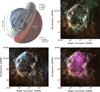 |
Fig. 1 Overview of the SNR IC443. Top-left panel: schematic drawing of the SNR morphology. The two-shell model proposed by Troja et al. (2006) is shown as a colored background image: the gray torus represents the molecular cloud discovered by Cornett et al. (1977) and is highlighted by white curved lines based on the higher resolution observations by Lee et al. (2012). The blue hemisphere labeled “subshell A” represents the shock front in the eastern region. In the northeast, where it has been confined by the encounter with the neutral H I cloud of Denoyer (1978), the ionic shock front is traced by optical, infrared and very soft X-ray emission (Alarie & Drissen 2019, dashed-dotted black lines). In the southern region, the thick black curved lines represent the areas of interaction with the molecular cloud and the shocked H2 ridges of Burton et al. (1988). The labels and positions of the different molecular clumps identified by Denoyer (1979b) and Dickman et al. (1992) are indicated with capital letters (B, C, D, E, F, G, H). The red hemisphere labeled “subshell B” represents the shock front in the western region, where it is expanding in a homogeneous and less dense medium. The position of the PWN discovered by Olbert et al. (2001) is indicated by a white star. The extension of the radio continuum halo is shown by dashed black lines (Lee et al. 2008, later confirmed by Castelletti et al. 2011). Locations and extensions of the four gamma-ray peaks at different energy ranges are indicated: EGRET centroid (∘), MAGIC centroid (□), VERITAS centroid (◊), and Fermi LAT centroid (∆), respectively measured by Esposito et al. (1996), Albert et al. (2007), Acciari et al. (2009) and Abdo et al. (2010). The respective localization errors are shown as crosses of size 0.5 σ. We note that the high-energy emission is extended, and hence the relation between Fermi LAT, VERITAS, and MAGIC observations may be better characterized by the extent of the emission rather than the centroids. The sizes of typical instrumental beams are indicated in the bottom-right corner of the figure. The other panels represent color composite images of IC443, with H I 21 cm line emission (Lee et al. 2008) in yellow and 24 µm (Spitɀer/MIPS) emission in white in all three panels. The third color channel represents a distinct signal in each panel: top-right panel: 12CO J = 1–0 (Lee et al. 2012, green); bottom-left panel: DSS optical observations (York et al. 2000, blue); bottom-right panel: XMM-Newton observations at 1.4–5 keV (Greco et al. 2018, purple). |
3.3 Spitzer/IRS SH versus SL map comparison
The H2 υ = 0–0 S(2) line was mapped both by the SH and SL modules. Hence, we could estimate the uncertainty introduced by the noisy vertical stripe (see Fig. A.1). The relative difference between the total flux of the S(2)[SH] and S(2)[SL] maps is ~5.5% (with ISL > ISH). We performed a pixel-per-pixel comparison of the S(2) spectral-line maps to estimate the uncertainty associated with the data (see Fig. 4). The left panel displays a small number of obvious outliers in the SL map (for ISL = [100−125] × 10−5 erg cm−2 s−1 sr−1 and ƒSH = [15–35] × 10−5 erg cm−2 s−1 sr−1) that are related to the noisy vertical stripe. These outliers were removed by the preprocessing transformations that we applied to the spectral-line maps (see Appendix A, and right panel of Fig. 4). In order to obtain a first estimate of the systematic and random uncertainties on the integrated intensity, we measured the statistical variables that describe the relation between the SL map and the SH map. First, we modeled the sample of data points ƒSL = f (ISH) by a linear function x ↦ ax + b. Then, we computed the standard deviation between the model Imod and the SL data points ISL. The results are presented in Table 2. Our pre-processing transformations enhanced the signal-to-noise ratio and reduced the systematic uncertainties (with respect to the raw SL maps).
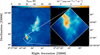 |
Fig. 2 Finderchart of the Spitɀer/IRS field of observations. Left: 12CO J = 2−1 10′ × 10′ map of the peak temperature obtained with the IRAM-30m telescope at an angular resolution of 11″.2 (Dell’Ova et al. 2020). Right: H2 υ = 0–0 S(1) map of the integrated line intensity obtained with Spitɀer/IRS. |
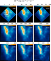 |
Fig. 3 H2 υ = 0–0 S(0) to S(7) pre-processed maps obtained with Spitɀer/IRS toward the region IC443G. The S(1) to S(7) maps were convolved to the spatial resolution of the S(0) map (8″.3, see Sect. 4.2). The S(0) line was mapped by the LH module, the S(1) and S(2) lines were mapped by the SH modules, and the rest were mapped by the SL module. The S(2) line was mapped by both the SH (top row) and SL (second row) modules. The coordinates of the field of observations are indicated in Fig. 2. Raw maps are shown in Fig. A.1. The array of white circles indicates the positions in which we extracted the signals of the S(0) to S(7) spectral-line maps to produce the population diagram mosaics presented in Fig. 5 (model 1: standard LTE approach) and Fig. 9 (model 2: H2 thermal admixture model). The size of the circles corresponds to the angular resolution of the S(0) observations, that is, 8″.3 in diameter. |
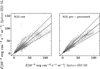 |
Fig. 4 Pixel-per-pixel comparison of the integrated intensity S(2) maps measured by the Spitɀer/IRS SH and SL modules before (left panel) and after pre-processing (rightpanel). The solid lines represents the 1:1 relation expected if the SH and SL data arrays were identical, and the dashed lines represent the ±25% relative errors. |
3.4 Spitɀer/IRS versus ISO comparison
The H2 S(2) to S(7) rotational lines were also observed with ISO (Cesarsky et al. 1999). In order to check the reliability of the data, we compared the Spitɀer/IRS and ISO measurements toward the positions A, B, and C (Table 1 of Cesarsky et al. 1999). We found an average relative error of 26% between the IRS and ISO spectra. To take this discrepancy in our study into account, we defined the uncertainties on any IRS measurements Iν∆ν as follows:
 (1)
(1)
where σMAD is the mean absolute deviation measured in the background of each spectral map. Therefore, the total uncertainty is representative of both the intrinsic noise of the images (σMAD) and the absolute flux calibration errors suggested by the discrepancy between the ISO and IRS measurements (26%).
4 Two-temperature model
We aim to produce maps of the column density and excitation temperature of the molecular phase toward the shocked clump IC443G. Our main goal is to provide a measurement of the H2 column density  that accounts for the mass of cold gas. To this end, we first performed a two-temperature population diagram analysis of H2 lines in each pixel of the Spitɀer/IRS spectral-line maps.
4.1 Assumptions
(i) Line opacity. We assumed that the emission of the pure rotational lines S(0) to S(7) is in the optically thin regime. Given the low Einstein coefficients Aul of the quadrupolar transitions of H2 (see Table 1), the emission of H2 rovibrational transitions remains optically thin even in proto-planetary disks, where the H2 column density can be larger than 1023 cm−2 (e.g., Bitner et al. 2008).
(ii) Thermalization. We assumed that the gas is at local thermodynamic equilibrium (LTE). This condition is verified if the local medium is sufficiently dense for a collisional equilibrium to settle, that is, if the following condition on the local density n is satisfied:
 (2)
(2)
 (3)
(3)
where Aul and Cul are respectively the Einstein coefficient of spontaneous emission and the collisional de-excitation rate. Wrathmall et al. (2007) presented the results of calculations of the collisional rate coefficients of H2 for a kinetic temperature T = 1000 K, T = 2500 K, and T = 4500 K. To test our assumption, we combined their calculations of Cul with the Aul coefficients shown in Table 1 to estimate the critical density ncrit of the H2 pure rotational lines. Depending on the kinetic temperature, the critical density of the S(7) line is ncrit ~ 1 × 10⁴−4 × 105 cm−3 (C97 (1000 K) = 4.6 × 10⁻¹³ cm3 s−1; C97(4500 K) = 1.9 × 10⁻¹¹ cm3 s−1). The critical densities of the other lines are lower. Cesarsky et al. (1999) estimated a pre-shock density ~104 cm−3 in the clump G. Thus, the low-J H2 lines are likely thermalized, although the high-J H2 lines might not be (see also van Dishoeck et al. 1993; Shinn et al. 2011). Assuming a density compression ratio of 10, all the lines would be thermalized in the post-shock.
(iii) Extinction. The scattering and absorption of incident photons by interstellar dust is expected to cause the extinction of H2 lines (e.g., Draine 2011). The S(0) to S(7) lines are characterized by λul = 5.5–28.2 µm (Table 1), a wavelength range in which the extinction is potentially non-negligible, depending on the magnitude of the visual extinction (Aυ). For a given wavelength λ, the observed intensity ƒ is related to the emitted signal I0 by the following equation:
 (4)
(4)
where Aλ is the extinction at wavelength λ. This equation is correct when the extinction is caused by a screen external to the source, which is the case here. The quantity Aλ/Aυ can be found in Rieke & Lebofsky (1985) for λ = 4.8, 7.0, 9.7, 14.3, 19, 30 µm. We performed a bicubic interpolation of this sample of data points to obtain the quantity Aλ/Aυ for the exact wavelength corresponding to each H2 pure rotational line. Following Shinn et al. (2011), we adopted a visual extinction Aυ = 10.8, inferred from A2.12 = 1.3, obtained by Richter et al. (1995), employing the ‘Milky Way, Rυ = 3.1’ extinction curve. Our correction of the extinction alters the flux by a few percentage points only.
(iv). We assumed a standard H2 ortho-to-para ratio (o/p = 3). We discuss the impact of choosing a different ortho-to-para ratio below.
4.2 Pixel-per-pixel method
Using Gaussian kernels, we first convolved the S(1) to S(7) maps (λ = 5.5−17 µm) to the spatial resolution of the S(0) map (8″.3 at λ = 28.2 µm). We then applied the following steps in each pixel (x, y) of the maps: (1) Correct the integrated intensity of each pixel for dust extinction (Eq. (4)). (2) Convert the integrated intensity I into an upper-level population Nup (Eq. (B.3)). (3) Build the population diagram, that is, log(Nup/𝑔up) with respect to Eup, where 𝑔up includes the nuclear spin degeneracy (2I + 1)(2J + 1), where I = 0/1 for J even/odd (cf. Table 1), and infer the column density and temperature from the linear fit of the data points.
4.3 Results: Population diagrams
We performed a systematic population diagram analysis in each pixel of the Spitɀer/IRS spectral-line maps. We performed two separate linear fits of the H2 energy levels respectively traced by the S(0), S(1), S(2) and S(3), S(4), S(5), S(6), S(7) lines to take into account temperature stratification (see the following developments). The results of our analysis are presented in Fig. 5. We extracted nine population diagrams in different locations of the IC443G clump (these locations are indicated in Fig. 3, first panel). We selected regions with low signal-to-noise ratios (first column of the mosaic) and regions with high signal-to-noise ratios (third column of the mosaic). The diagrams are shown in Fig. 5. In order to check the quality of the best-fits, we performed a chi-square test on the data points, defined by the reduced chi-square (or chi-square per degree of freedom):
 (5)
(5)
where Nup is the column density; f is the adopted linear model (which is distinct for the energy levels traced by the S(0)–S(2) and S(3)–S(7) lines, following our decomposition into two components); σ(Nup) is the uncertainty on Nup derived from Eq. (1); and N = 8 is the number of data points. Lastly, p = 4 is the number of free parameters (i.e., the excitation temperature and total column density for the warm and cold components). In the extracted population diagrams, χ2 varies between 0.95 and 2.67 (see Fig. 5). The value of χ2 increases for the high signal-to-noise beams (3, 6, 9) since the small error bars make the data harder to reproduce with our model. The linear fit of the Jup = 5–9 upper levels (gray curve in Fig. 5) systematically fails to reproduce the column density of the population level Jup = 2. Conversely, the linear fit of the remaining data points (Jup = 2–4, red curve) does reproduce the lower energy levels, although it is completely off for higher energy levels. Classically, at least two excitation temperatures are required to reproduce the H2-level populations with a ‘cold’ component (dominating levels Jup = 2–4) and a ‘warm’ component (dominating levels Jup = 3–9). We found, however, that the levels J = 3 and J = 4 are not well reproduced by our two-temperature model, which we interpret as evidence that a continuous distribution of temperature would better represent the data than a bimodal distribution. Naturally, the total column density is given by the sum of the column densities inferred from each component (‘warm’ and ‘cold’).
4.4 Discussion
We have obtained an estimate of the total H2 column density inferred from the emission of the S(0) to S(7) lines (see Table 3, first and second rows). The fit of the S(0), S(1), S(2) (in red in Fig. 5) traces the ‘cold component’ of H2 (Tex = 370–470 K,  cm−2) and the bulk of the molecular mass. Similarly, the fit of the S(3), S(4), S(5), S(6), S(7) (in gray in Fig. 5) traces the ‘warm component’ of H2 (Tex = 740–840 K,
  cm−2). As expected, the transitions of H2 cannot be reproduced by a single excitation temperature; hence, our results indicate that the medium is characterized by thermal stratification along the line of sight. Both the column density and excitation temperature increase toward the shocked clump: low signal-to-noise beams (1, 4, 7) are characterized by a column density
  cm−2 and temperature Tex ~ 370 K (for the cold component), while the high signal-to-noise beams (3, 6, 9) are characterized by a column density
  cm−2 and temperature Tex ~ 470 K (for the cold component).
The energies Eup of the upper levels (J = 2–9) are 510–7200 K (Table 1). It is unlikely that the result of our analysis yields the total H2 column density since the rotational energy levels J = 0 and J = 1 are expected to hold the greater part of the ‘cold mass’ of molecular hydrogen and perhaps another component should be considered for the first two levels. In other words, it is likely that these two levels are not thermalized with the others. It is well known that the ‘standard’ population diagram analysis of H2 pure rotational lines is a poor method to measure the total column density. Roussel et al. (2007) presented results of the analysis of warm H2 lines in the Spitzer SINGS (Spitzer Infrared Nearby Galaxy Survey) galaxy sample. Under a conservative assumption about the distribution of temperatures, they found that the column densities of warm H2 derived from Spitzer/IRS observations amount to between 1% and 30% of the total mass of H2 (their estimate of the mass of cold H2 was derived from velocity-integrated 12CO J = 1–0 observations). Therefore, it is possible that our estimate of the H2 column density from the sum of the 'gray' and 'red' fits (Fig. 5) lies between 1% and 30% of the true column density.
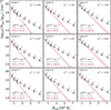 |
Fig. 5 Population diagrams extracted from the positions shown in Fig. 3. The corresponding positions are indicated in the top-left corner of each panel. The black data points represent the Nup measurements and their uncertainties. The gray curve represents the linear model obtained for the S(3) to S(7) transitions. The red curve represents the linear model obtained for the S(0) to S(2) transitions. Gray circles represent the sum of the two models for each transition. The errors associated with the best linear models are represented by a filled area around the curves. The corresponding excitation temperatures are shown in the bottom-left corner of the diagrams ('cold' component in red and 'warm' component in gray). The total column density is also shown (in black). The results of the χ2 test (see text and Eq. (5)) are presented in the top-right corner of the diagrams. The order of the diagrams (from left to right and top to bottom) is the same as the order of the white circles in Fig. 3. |
Results of our analysis of the H2 S(0) to S(7) pure rotational lines.
5 Thermal admixture model
5.1 Assumptions
Following the method presented by Neufeld & Yuan (2008, referred to as the H2 thermal admixture model), we assumed that the molecular hydrogen probed along a line of sight has a column density that can be described by the following power-law distribution with respect to the kinetic temperature of H2 (denoted T):
 (6)
(6)
where Λ and Γ are two constants. If Γ is known, Λ can be determined by integrating Eq. (6) between Tmin and Tmax:
 (7)
(7)
This power-law description is driven by the observation that the population diagrams shown in Fig. 5 are better described by two components than a single Tex (the 'cold' and 'warm' components). Equation (6) is a continuous generalization of this multi-temperature analysis. We assumed that the emission of the H2 lines is produced by a mixture of gas temperatures (both along the line of sight and possibly across the plane of sky probed by the beam of Spitzer/IRS). Our adopted description (Eq. (6)) relies on the physical assumption that the shocked medium is stratified in temperature in a way that can be reproduced by a power-law distribution between a minimum gas temperature (Tmin) and a maximum gas temperature (Tmax). This assumption is supported by the expected temperature profile in a parabolic C-type bow shock in steady state (Shinn et al. 2011; Smith & Brand 1990). If we fix Tmin and Tmax, we have the same amount of parameters to fit as in the previous section (alin, blin in the standard population diagram model and Λ, Γ in this model). Once Tmin and Tmax are fixed, the two remaining parameters of this model are the steepness of the distribution (the power-law index Γ) and the total H2 column density Ntot(T ≥ Tmin). The value of Tmax has a marginal effect on the resulting H2 column density since most of the mass is held by cold gas. Based on the excitation temperature maps found previously (see Fig. 5), we first fixed Tmax = 1500 K. We then verified that higher temperatures do not modify the results (up to Tmax = 4000 K, the temperature at which H2 is rapidly dissociated in a shock, Le Bourlot et al. 2002). Determining the correct value of Tmin is paramount since it controls the column density of H2. We can estimate the lower boundary of the temperature distribution based on the results of our previous pixel-per-pixel radiative transfer analysis of 12CO and 13CO J = 1−0, J = 2−1 and J = 3−2 lines (Eup = 5.5, 16.6, 33.2 K), where we found that the temperature of the cold gas is  across the inner regions of the shocked clump (Dell'Ova et al. 2020). Hence, we fixed Tmin(H2) = 25 K accordingly with the average temperature of the molecular gas determined toward the shocked clump, and then we estimated the error on the derived H2 column density by comparing our results with complementary models obtained with Tmin = 15 K and Tmin = 40 K.
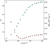 |
Fig. 6 Average chi-square (‘χ2’, i.e., the average chi-square across the map, indicated by red diamonds) and average column density ( |


5.2 Method: LTE and non-LTE admixture models
Based on the power-law description of the temperature distribution, we experimented with two distinct admixture models. The first model assumes LTE. The assumptions and discretization method are described in Appendix B. The second model is based on statistical equilibrium (hereafter SE). We used the code developed by Gusdorf et al. (2008) and Godard et al. (2019). This code computes the excitation and radiative transfer in a collection of gas slabs defined by the user. Our modeled gas consists of H2, H, He, and electrons only, with n(H) = 10−2 n(H2), n(He) = 0.2 n(H2), and n(e−) = 10−7 n(H2). In order to account for possible deviations from LTE, we performed a series of calculations with variable H2 local density, between  and
and  (see Fig. 6, where we show the variation of the average chi-square and average column density within the map with respect to the adopted local density). For each model, the remaining free parameters were the column density and the kinetic temperature.
We produced a discrete parameter grid [Γ, Ntot(T ≥ Tmin)] for each model. We then performed a chi-square test to compare the observations of H2 lines to the integrated intensity models. We measured the following quantity in each cell of the model grid:
 (8)
(8)
where sJ→J–2 is the integrated intensity measurement corrected for dust extinction (see previous section), mJ→J–2 is the modeled integrated intensity (Eq. (B.7)), σJ→J–2 is the uncertainty (derived via Eq. (1)), and N = 8 is the number of data points. Lastly, p = 2 is the number of free parameters (the power-law index and total column density). The best-fit was then found by locating the minimum;χ2 value in the array resulting from the chi-square test.
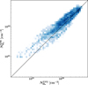 |
Fig. 7 Pixel-per-pixel comparison between the column densities derived from our best LTE and non-LTE thermal admixture models. The blue color map is a linear representation of the number of counts in the bins. The non-LTE model shown here was computed assuming a local density of n = 2.5 × 105 cm−3 (we explored a range: n = 104−107 cm−3). |
5.3 Results
We performed a chi-square test based on Spitzer/IRS mapping observations of the S(0) to S(7) lines and their comparison with model grids, adopting the parameter boundaries Γ = 0,5-5 (linearly spaced) and Ntot(T ≥ Tmin) = 1020–1024 cm–2 (logarithmically spaced), and we explored a range of local densities  with our non-LTE approach. A direct comparison between our LTE and non-LTE results is shown in Fig. 7. The results of the non-LTE admixture model are presented in Figs. 6, 8, 9, and 10. All the pixels across the spectral maps have been reproduced within a confidence level of 3σ by the LTE and non-LTE models.
Our best-fit non-LTE model corresponds to a local density n = 2.5 × 105 cm–3 (see Fig. 6); hence, we fixed the input density to this value, which explains the small discrepancies between our LTE and non-LTE results (see Fig. 7). In Fig. 8, we present the chi-square grids resulting from the application of Eq. (8) toward the same locations as presented in Fig. 3 and which we initially analyzed in the previous section. The chi-square grids shown in the first column of the mosaic display the lowest ;χ2 values because they correspond to low signal-to-noise regions of the map; hence, sJ→J–2/σJ→J–2 is systematically lower and so is the product of Eq. (8). In all cases, the first black contour level (corresponding to  , where
  is the minimal value of ;χ2 across the model grid) indicates the values of Γ and Ntot that best reproduce the observations. We found that column densities of the order 1022 cm–2 and power-law indices Γ = 2.2–4.7 reproduce the observations, although with some degeneracy between the parameters. In IC443C, Shinn et al. (2011) found variations of Γ over the range 3-6, with the majority of sight lines in the range 4-5. In addition, they showed that spatially unresolved parabolic C-type bow shocks in steady state (Smith & Brand 1990) would produce a temperature stratification dN ∝ T–3.8dT (i.e., Γ = 3.8). One would expect Γ to get closer to this predicted value within the shocked clump, but our measurements show the opposite: Γ decreases toward the shocked clump, suggesting a variation in the shock physical conditions. In fact, it is likely that there is a mixing of physical conditions along the line of sight, including both cold quiescent gas and warm high-velocity shocked gas. In addition, using different temperature boundaries (Tmin, Tmax) has an impact on the value of Γ, and Shinn et al. (2011) performed their analysis with Tmin = 100 K, Tmax = 4000 K, so it contributes to the discrepancies with our measurements of Γ in IC443G.
Based on our determinations of the best-fit parameters [Γ, Ntot(T ≥ Tmin)] for each location of the map shown in Fig. 3, we built synthetic population diagrams (see Fig. 9) to compare our non-LTE results with the population diagrams presented in the previous section (Fig. 5). Toward these locations, the minimized;χ2 varies between 0.85 and 2.13. The systematic deviation of the Jup = 5 level population above our best-fit model indicates that our power-law distribution might be unable to reproduce the break between the dynamic of the lower-J level populations (tracing cold molecular hydrogen) and the rest of the data points.
Additional tests and remarks. (i) We tried to modify the fixed parameter Tmax from 1500 K to 2000 K, 3000 K and 4000 K to check how the best-fit is modified. These modifications increase the average ;χ2, and they have little effect on the total H2 column density (the relative difference is lower than 10%). Therefore, we kept our initial Tmax. (ii) Similarly, we tried to adopt a lower value of Tmin (down to 10 K), which increased the average ;χ2 as well. (iii) We adopted a standard H2 ortho-to-para ratio (o/p = 3) and checked that a two-fold variation in the ortho-to-para ratio has a negligible impact on the best-fit column density (less than 2%).
(i) Total column density map. The column density map obtained from the comparison of the S(0) to S(7) transitions with our model grid is shown in the left panel of Fig. 10. The column density varies between N ~ 1021 cm–2 and N ~ 6 × 1022 cm–2 between the outer edges and the core of the clump G. The peak column density is approximately 40 times higher than with the two-temperature population diagrams.
(ii) Average temperature map. The average temperature map obtained from the comparison of the S(0) to S(7) transitions with our model grid is shown in the right panel of Fig. 10. The average temperature map is produced by determining the contribution of each layer of molecular hydrogen to the temperature measured along the line of sight and dividing by the total column density:
 (9)
(9)
The average temperature varies between T ~ 60 K and T ~ 140 K; hence, we succeeded in tracing colder gas. The spatial distribution of the temperature is uncorrelated to the column density map, and several localized ‘warm spots’ were found both within the clump and on the outer edges. We discuss the nature of these warm spots in Sect. 6.4.
(iii) H2 temperature tomography. Since we had determined the best-fit parameters (Λ, Γ), Eq. (B.4) allowed us to build the partial column density of a layer of molecular hydrogen at any temperature Tmin ≤ Tlayer ≤ Tmax. Using ΔT = 15 K and ΔT = 150 K temperature bins (respectively in the intervals 25–925 K and 925–1500 K), we built a partial column density map mosaic, shown in Fig. 11. This figure shows the variation in column density with respect to the temperature of distinct ther-malized layers of molecular hydrogen along the line of sight. We observed that the very high temperature molecular hydrogen (fourth row: T = 925–1500 K) is more clumpy than the warmer molecular hydrogen (second row: T = 325–475 K). The coldest molecular hydrogen (first row: T = 25–100 K) is also clumpy and more extended, and it has a higher column density. These maps show that the cold molecular hydrogen holds the bulk of the mass. The morphology of the warm gas (second and third rows: T = 325–925 K) is well correlated to the S(0) to S(2) lines, whereas the clumpy morphology of the hot gas (fourth row: T = 925–1500 K) is more correlated to the S(3) to S(7) lines (see Fig. 3 for comparison).
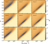 |
Fig. 8 Results of the chi-square test applied to our observations and the non-LTE model grid of the S(0) to S(7) H2 lines integrated intensities (see Eq. (8)). Each panel of the mosaic corresponds to the panels shown in Fig. 9 (positions indicated in Fig. 3). The term Γ is the power-law index, and Ntot is the total column density for T > Tmin = 25 K (see Eqs. (6) and (7)). The background color indicates the absolute value of χ2, and the set of black contours indicate the inner areas corresponding to the 1σ, 2σ, and 3σ levels, that is, |
![${\chi ^2} \le \left[ {1.17{\chi _{{{\min }^2}}},1.67{\chi _{{{\min }^2}}},2.5{\chi _{{{\min }^2}}}} \right]$](/articles/aa/full_html/2024/05/aa47984-23/aa47984-23-eq41.png)

![$(\Delta {\chi ^2}(n\sigma ) = [1 + n/(N - p)]\chi _{\min }^2$](/articles/aa/full_html/2024/05/aa47984-23/aa47984-23-eq43.png)
6 Discussion
We have estimated the total H2 column density and temperature maps from the analysis of the S(0) to S(7) pure rotational lines using three distinct models: a two-temperature description, an LTE admixture, and a non-LTE admixture (results are shown in Table 3, in which the uncertainty on Tmin has been taken into account for the estimate of the column density  and mass
  ). Comparison between our three models shows that with respect to the thermal admixture model, the ‘standard’ LTE analysis of the Spitzer/IRS H2 lines might underestimate the total column density by ~97% in the region IC443G, which would be consistent with the conclusions of Roussel et al. (2007) in nearby galaxies (they found that between 1% and 30% of the total column density is traced by the allowed rotational transitions). Nonetheless, the true temperature distribution of the gas remains unknown, and the discrepancy between our models is mainly representative of the uncertainty associated with our assumptions.
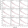 |
Fig. 9 Population diagrams extracted from the positions shown in Fig. 3 and corresponding to the chi-square test shown in Fig. 8. The black data points represent the Nup measurements and their uncertainties. The red circles represent the best-fit non-LTE model obtained for the S(0) to S(7) transitions. The corresponding power-law indices and total column densities are shown in the bottom-left corner of the diagrams. The results of the χ2 test (see text) are presented in the top-right corner of the diagrams. The order of the diagrams (from left to right and top to bottom) is the same as the order of the white circles in Fig. 3. |
6.1 Local density in IC443G
We aim to infer an estimate of the local density from the total H2 column density, and we propose an approximate geometrical model for the shocked clump (for the sake of simplicity). We describe this structure by a cylinder of length l = 3′ and diameter D = 1′. At a distance of 1.8 kpc (Ambrocio-Cruz et al. 2017; Yu et al. 2019), this corresponds to 1–1.5 pc and D = 0.5 pc. Assuming that other sources of emission along the line of sight are negligible, the local density is given by the ratio of the measured column density and the length of shocked clump crossed. Hence, we have  . The local density would be larger toward unresolved knots of H2. In fact, if we assume that in any line of sight, all H2 molecules are confined in a single quasi-spherical knot of diameter ~0.1 pc (~10″), then we would have
  . Assuming Tkin = 1000 K, our first estimate (
 ) implies that the S(6) and S(7) lines might not be fully thermalized. The second estimate (
 ) is consistent with the minimization of the local density in our non-LTE models (see Fig. 6), and it implies a thermalization of the S(0) to S(6) lines at Tkin = 1000 K.
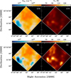 |
Fig. 10 Resulting images from the LTE and SE analyses. Top panel: column density (left) and excitation temperature (right) derived from the analysis of the S(0) to S(7) H2 pure rotational lines, following the LTE method described in Sect. 5.2. Bottom panel: column density (left) and kinetic temperature (right) derived from the SE analysis described in Sect. 5.2. |
6.2 Gas mass in IC443G
We estimated the H2 molecular gas mass in IC443G by summing up all pixels in our column density map (see Fig. 10):
![${M_{{{\rm{H}}_2}}} = 2{m_{\rm{u}}}\sum\limits_{i,j} {{N_{{{\rm{H}}_2}}}} [i,j]\Delta s,$](/articles/aa/full_html/2024/05/aa47984-23/aa47984-23-eq50.png) (10)
(10)
where ![${N_{{{\rm{H}}_2}}}[i,j]$](/articles/aa/full_html/2024/05/aa47984-23/aa47984-23-eq51.png) is the column density of a pixel (i, j), Δs[cm2] ≃ 1.5 × 10¹⁰ ΔΩ[″]dkpc is the physical (sky) surface of a pixel, and mu ≃ 1.66 × 10⁻²⁷ kg is the atomic mass unit. Assuming dkpc = 1.8 ± 0.2 (Ambrocio-Cruz et al. 2017; Yu et al. 2019) and taking into account the uncertainty on the cold gas temperature (
is the column density of a pixel (i, j), Δs[cm2] ≃ 1.5 × 10¹⁰ ΔΩ[″]dkpc is the physical (sky) surface of a pixel, and mu ≃ 1.66 × 10⁻²⁷ kg is the atomic mass unit. Assuming dkpc = 1.8 ± 0.2 (Ambrocio-Cruz et al. 2017; Yu et al. 2019) and taking into account the uncertainty on the cold gas temperature ( ), we obtained a mass
  (solar masses). This mass measurement does not correspond to the total mass of the shocked clump since the Spitzer/IRS field of observations does not cover the entire structure (see Fig. 2). We note, however, that our measurement is consistent with the shocked clump mass estimate inferred from our 12CO observations (performed in a 10′ × 10′ box),
  (Dell’Ova et al. 2020).
6.3 H2-to-12CO abundance
Using a Gaussian kernel, we re-convolved and re-sampled our H2 column density map into the same angular resolution and spatial grid as our IRAM-30m and APEX 12CO column density maps (Fig. 2; Dell'Ova et al. 2020). A total of 54 pixels can be directly compared between the two column density maps, all characterized by high signal-to-noise ratios (s/n ≥ 6). The pixel-per-pixel comparison between the H2 and 12CO column density maps is shown in Fig. 12. We found a quasi-linear relation between the column densities, and the H2-to-12CO column density ratio estimated from the linear fit is 3.6 × 10⁴. The inferred ratio is in agreement with the standard value derived from visual extinction studies in molecular clouds, albeit a bit higher ( Dickman 1978; Frerking et al. 1982). Toward the shocked clump, it is possible that ionization might decrease the 12CO abundance with respect to H2 via the conversion of 12CO into C+, C, CH3OH, or CH4, resulting in a departure from
  In order to prepare a future study of the chemistry in IC443G, we report the values of
  and
and  toward two positions using variable beam sizes in Tables 4 and 5.
6.4 Young stellar object candidates
In Fig. 13, we compare the spatial distribution of young stellar object candidates (YSOs) with the H2 temperature map derived from our non-LTE analysis. This sample of YSO candidates was selected using color-color filtering of WISE and 2MASS infrared point sources (Dell’Ova et al. 2020). We used the Python package mistree to produce the minimal spanning trees corresponding to our samples of point sources (Naidoo 2019). The minimal spanning tree is defined as the network of lines, or branches, that connect a set of points together such that the total length of the branches is minimized and there are no closed loops (Cartwright & Whitworth 2004; Gutermuth et al. 2009). We found signs of clustering along the warm shocked clump and that a few point sources are correlated with hot knots of gas. We assumed that a few protostars could contribute to the localized heating shown in our map. In Fig. 13, there is only one warm spot that is not associated with a YSO candidate (to the eastern end of the Spitzer/IRS maps). We checked the XMM-Newton observations between 0.4 keV and 7.2 keV (Troja et al. 2006) for a local source of X-ray radiation in this area, and we found a source with a ~20″ shift with respect to the warm spot (see Fig. B.1). It is still possible that one or several embedded Class 0 protostar(s), which cannot be detected from color-color filtering of WISE and 2MASS infrared point sources, could be the cause of the heating toward this eastern position. It is important to note that associations between these point sources and the SNR IC443 can be coincidental. Additionally, considering the protostellar collapse phase timescale of approximately ~105 yr (e.g., Lefloch & Lazareff 1994), we cannot conclude that the mid-infrared point sources are unequivocally linked to YSOs triggered by the IC443 SNR. In fact, these YSO candidates may belong to the same generation as the progenitor of the supernova, which may have evolved more rapidly due to its increased mass.
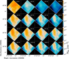 |
Fig. 11 Tomographic representation of |

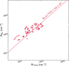 |
Fig. 12 Pixel-per-pixel comparison of the 12CO and H2 total column density maps. The maps are restricted to the field of observations mapped by both Spitzer/IRS, IRAM-30m, and APEX telescopes. The 12CO data points were obtained with opacity-corrected population diagrams Dell’Ova et al. (2020). The H2 data points correspond to the results obtained with the thermal admixture SE description (see Sect. 5.2). We show the best linear fit associated with the sample of data points and the corresponding H2-to-12CO molecular abundance. |
H2 and 12CO column density measurements toward 6h 16m , 22°32′15″.

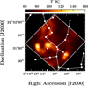 |
Fig. 13 Gas temperature map derived from our non-LTE thermal admixture model. The 2MASS and WISE young stellar object candidates are represented by a minimal spanning tree. |
7 Summary
We performed an analysis of the Spitzer/IRS H2 spectral-line maps toward the IC443G region. Our main findings are the following:
(a) The level populations traced by the H2 S(0) to S(7) pure rotational lines cannot be reproduced by a single excitation temperature. This is as expected. When a mixture of shock velocities is involved, the shocked clump is stratified in temperature. Thus, using a power-law distribution of temperatures better represents the data, although it remains an approximation that cannot account for the complex mixing of physical conditions in IC443G, where the emission is driven by both cold quiescent gas and warm high-velocity shocked gas. In fact, even a single shock model may struggle to precisely replicate the observations, primarily because different shocks can be present within the observational beam, as discussed by Kristensen et al. (2023).
(b) Assuming that the temperature distribution of H2 spans the range 25–1500 K, our thermal admixture model allows (within a confidence level of 3σ) the level populations to be successfully reproduced, with a power-law index Γ ~ 2.2–4.7, although with a substantial degeneracy between Γ and the total column density  . In IC443C, Shinn et al. (2011) showed that parabolic C-type bow shocks in a steady state can produce such power-law temperature stratification, as had been proposed for other shocked regions by Smith & Brand (1990). In this scenario, spatial variation of Γ across our field of observation would correspond to variations in the distributions of velocities at the head of unresolved bow shocks. Our average estimate of Γ is below the value predicted by shock models (Γ ~ 3.8). We note, however, that our degenerate model (see Fig. 8) is consistent with Γ ~ 3.8. More importantly, Shinn et al. (2011) used different temperature boundaries to predict this value of Γ.
(c) The total column density of H2 inferred from our two-.temperature excitation diagram accounts for approximately 3% of the total column density deduced from our thermal admixture model. Our analysis shows that an estimate of the cold molecular gas temperature is paramount to constraining the total H2 mass. The 12CO rotational transitions, thanks to their low-temperature energy levels (E1 = 5.53 K, E2 = 16.6 K, E3 = 33.2 K), can provide such a temperature estimate. We acknowledge, however, that small inaccuracies in the assumed boundaries and shape of the temperature distribution may result in significant errors for the derived column densities.
(d) The agreement between the observations and our thermal admixture model suggests that the S(0) to S(7) H2 lines could be thermalized. However, the local density inferred from our column density measurement is in the range 0.2−2 × 105 cm−3, depending on the adopted geometry. Our χ2 -minimization also suggests a local density of n = 2.5 × 105 cm−3. This range of. local densities is not consistent with a full thermalization of the S(6) and S(7) lines.
(e) Taking into account the uncertainty on the minimal temperature of the gas ( K, estimated from 12CO observations), we measured a molecular gas mass
  M⊙ across the Spitzer/IRS field of observations. This measurement represents a lower bound of the mass of protons available for CRs to interact with in IC443G since there is also atomic gas along the line of sight (Lee et al. 2008).
(f) We compared our findings with the analysis of 12CO rotational lines toward IC443G (Dell’Ova et al. 2020). Our mea. surements are consistent with a H2-to-12CO abundance ratio of 3.6 × 10⁴, indicating that some of the carbon may exist in the form of C or C+ in this region.
The analysis of the Spitzer/IRS H2 spectral-line maps toward the IC443G region provides an insight into the complex dynamics of shocked molecular gas. The observed temperature distribution, reflecting both quiescent and shock-excited components, emphasizes the need for shock models to capture these dynamics fully. Additionally, our findings stress the importance of accounting for multi-temperature environments when attempting to measure the gas mass. Future work should focus on comprehensive shock modeling and higher resolution observations, to disentangle the emission of protostellar outflows from the large-scale shock structure.
Acknowledgements
This project has received funding from the French Agence Nationale de la Recherche (ANR) through the project COSMHIC (ANR-20-CE31-0009), and the French Programme National de Physique et Chimie du Milieu Interstellaire (PCMI) of CNRS/INSU (with INC/INP/IN2P3).
Appendix A Description of the pre-processing transformations: Systematic noise reduction
Using Python, we applied the following pre-processing steps to. the Spitzer/IRS spectral-line maps:
- 1.
The S(0) spectral-line map is strongly affected by the continuum emission of two stars at α[J2000] = 6h16m41s, δ[J2000] = 22º30′58″ and
![${\alpha _{[{\rm{J}}2000]}} = {6^{\rm{h}}}{16^{\rm{m}}}{44^{\rm{s}}}.5$](/articles/aa/full_html/2024/05/aa47984-23/aa47984-23-eq84.png) , δ[J2000] = 22º31′33″. We used two 2D Gaussian functions (G1, G2, re-normalized between zero and one) and the S(1) map as an emission model to remove these components in the pixels (x, y):
, δ[J2000] = 22º31′33″. We used two 2D Gaussian functions (G1, G2, re-normalized between zero and one) and the S(1) map as an emission model to remove these components in the pixels (x, y):
![$\matrix{ {} & {{S^0}(x,y) = {S^0}(x,y)\left[ {1 - \left( {{G_1}(x,y) + {G_2}(x,y)} \right)} \right]} \cr {} & {\quad + M \times {S^1}(x,y)\left[ {{G_1}(x,y) + {G_2}(x,y)} \right],} \cr } $](/articles/aa/full_html/2024/05/aa47984-23/aa47984-23-eq85.png) (A.1)
(A.1)where S0 and S1 are respectively the S(0) and S(1) maps, and M = median(S0/S1) is a re-scaling factor.
- 2.
The S(6) spectral-line map has the most severe horizontal stripes (see Fig. A.1). We used the S(5) map as an emission model to isolate the emission from the stripes and generate a noise model N(x, y) from a data array initially filled with. zeros:
![$\alpha (x,y) = \left[ {{S^6}(x,y)/\max \left( {{S^6}} \right) - {S^5}(x,y)/\max \left( {{S^5}} \right)} \right]$](/articles/aa/full_html/2024/05/aa47984-23/aa47984-23-eq86.png) (A.2)
(A.2)
 (A.3)
(A.3)where S6 and S5 are respectively the S(6) and S(5) maps, and αtreshold is an arbitrary threshold that controls the separation between the signal and the systematic stripes. The pre-processed S(6) map is then given by S6(x,y) = S 6(x,y) −N (x,y).
- 3.
All the SL maps (i.e., S(2) to S(7)) were systematically presenting a strong vertical stripe. This stripe was located on the columns 52 and 53 of the data arrays. To correct this artifact, we performed the following interpolation:
 (A.4)
(A.4)
 (A.5)
(A.5) - 4.
Using Gaussian kernels, we convolved the S(1) to S(7) maps to the resolution of the S(0) map
 . This convolution lowers the contribution from the horizontal stripes in all maps..
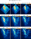 |
Fig. A.1 H2 v = 0 − 0 S(0) to S(7) raw maps obtained with Spitzer/IRS toward the region IC443G (Neufeld et al. 2004). The S(0) line was mapped by the LH module, the S(1) and S(2) lines were mapped by the SH modules, and the rest by the SL module. The S(2) line was mapped by both the SH (top row) and SL (second row) modules. The coordinates of the field of observations are indicated in Fig. 2. Pre-processed maps are shown in Fig. 3 |
The results of these pre-processing steps are presented in Fig. 3. The systematic vertical stripe as well as the horizontal stripes in the S(6) map have both been removed. The average flux variation across the map between the raw and pre-processed images is ~1.02%; hence it should not significantly modify the average results, and it is lower than the relative difference between the raw S(2)[SH] and S(2)[SL] maps (~5.5%).
Appendix B Thermal admixture model (LTE)
We built model grids of the integrated intensity for the S(0) to S(7) lines based on the H2 thermal admixture description. The H2 total column density at a temperature T = Tlayer (referred to as Ntot(T = Tlayer)) can be determined from Eq. 6 and Eq. 7. If we adopt the same LTE assumptions as in Section 4.1 for each layer of molecular hydrogen at a temperature Tlayer, then the upper-level populations can be derived from the Boltzmann distribution for Ntot(T = Tlayer):
 (B.1)
(B.1)
where 𝑔up is the degeneracy, Eup is the energy of the level, kB is the Boltzmann constant and T is the temperature of the gas, and Z(T) is the partition function defined by:
 (B.2)
(B.2)
The integrated intensity produced by the layer of molecular hydrogen can then be inferred from the following relation:
 (B.3)
(B.3)
where h is the Planck constant, νul is the frequency of the spectral line, and Aul is the Einstein coefficient for spontaneous. de-excitation. The sum of the integrated intensity contributions over the column density distribution yields an estimate of the integrated intensity measured along the line of sight.
Appendix B.1 Discretization of the column density distribution N(T)
The discretization of Eq. 6 yields
 (B.4)
(B.4)
where ∆N = Ntot(T = Tlayer) is the column density of a layer of molecular hydrogen at temperature T and ∆T = (Tmax − Tmin)/Nbin is a temperature bin (Nbin is the total number of bins). We produced a discretized column density distribution that satisfies the following condition:
 (B.5)
(B.5)
Appendix B.2 I(Λ, Γ) model grid
For a choice of parameter (Γ, Ntot(T ≥ Tmin)), we produced a model of the S(0) to S(7) lines integrated intensity by performing the following computations:
- 1.
Assuming LTE, we computed the upper-level populations of each molecular hydrogen layer, applying Eq. B.1:
 (B.6)
(B.6)where Z(T) is the partition function defined by Eq. B.2.
- 2.
Then, we computed the integrated intensity of the S(0) to S(7) lines produced by each layer of gas, applying Eq. B.3:
 (B.7)
(B.7)
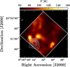 |
Fig. B.1 Gas temperature map derived from our non-LTE thermal admixture model. White contours represent hard X-ray emission (2–7.2 keV) detected by XMM-Newton (Troja et al. 2006)). |
References
- Abdo, A. A., Ackermann, M., Ajello, M., et al. 2010, ApJ, 712, 459 [NASA ADS] [CrossRef] [Google Scholar]
- Acciari, V. A., Aliu, E., Arlen, T., et al. 2009, ApJ, 698, L133 [NASA ADS] [CrossRef] [Google Scholar]
- Alarie, A., & Drissen, L. 2019, MNRAS, 489, 3042 [NASA ADS] [CrossRef] [Google Scholar]
- Albert, J., Aliu, E., Anderhub, H., et al. 2007, ApJ, 664, L87 [NASA ADS] [CrossRef] [Google Scholar]
- Ambrocio-Cruz, P., Rosado, M., de la Fuente, E., Silva, R., & Blanco-Piñon, A. 2017, MNRAS, 472, 51 [NASA ADS] [CrossRef] [Google Scholar]
- Bitner, M. A., Richter, M. J., Lacy, J. H., et al. 2008, ApJ, 688, 1326 [NASA ADS] [CrossRef] [Google Scholar]
- Braun, R., & Strom, R. G. 1986, A&A, 164, 193 [NASA ADS] [Google Scholar]
- Burton, M. G., Geballe, T. R., Brand, P. W. J. L., & Webster, A. S. 1988, MNRAS, 231, 617 [NASA ADS] [Google Scholar]
- Cartwright, A., & Whitworth, A. P. 2004, MNRAS, 348, 589 [Google Scholar]
- Castelletti, G., Dubner, G., Clarke, T., & Kassim, N. E. 2011, A&A, 534, A21 [NASA ADS] [CrossRef] [EDP Sciences] [Google Scholar]
- Cesarsky, D., Cox, P., Pineau des Forêts, G., et al. 1999, A&A, 348, 945 [NASA ADS] [Google Scholar]
- Cornett, R. H., Chin, G., & Knapp, G. R. 1977, A&A, 54, 889 [NASA ADS] [Google Scholar]
- Cosentino, G., Jiménez-Serra, I., Tan, J. C., et al. 2022, MNRAS, 511, 953 [NASA ADS] [CrossRef] [Google Scholar]
- Dabrowski, I. 1984, Can. J. Phys., 62, 1639 [NASA ADS] [CrossRef] [Google Scholar]
- Dell’Ova, P., Gusdorf, A., Gerin, M., et al. 2020, A&A, 644, A64 [NASA ADS] [CrossRef] [EDP Sciences] [Google Scholar]
- Deng, Y., Zhang, Z.-Y., Zhou, P., et al. 2023, MNRAS, 518, 2320 [Google Scholar]
- Denoyer, L. K. 1978, MNRAS, 183, 187 [NASA ADS] [CrossRef] [Google Scholar]
- Denoyer, L. K. 1979a, ApJ, 232, L165 [NASA ADS] [CrossRef] [Google Scholar]
- Denoyer, L. K. 1979b, ApJ, 228, L41 [NASA ADS] [CrossRef] [Google Scholar]
- Dickman, R. L. 1978, ApJS, 37, 407 [CrossRef] [Google Scholar]
- Dickman, R. L., Snell, R. L., Ziurys, L. M., & Huang, Y.-L. 1992, ApJ, 400, 203 [Google Scholar]
- Draine, B. T. 2011, Physics of the Interstellar and Intergalactic Medium (Princeton University Press) [Google Scholar]
- Endres, C. P., Schlemmer, S., Schilke, P., Stutzki, J., & Müller, H. S. P. 2016, J. Mol. Spectrosc., 327, 95 [NASA ADS] [CrossRef] [Google Scholar]
- Esposito, J. A., Hunter, S. D., Kanbach, G., & Sreekumar, P. 1996, ApJ, 461, 820 [NASA ADS] [CrossRef] [Google Scholar]
- Frerking, M. A., Langer, W. D., & Wilson, R. W. 1982, ApJ, 262, 590 [Google Scholar]
- Godard, B., Pineau des Forêts, G., Lesaffre, P., et al. 2019, A&A, 622, A100 [NASA ADS] [CrossRef] [EDP Sciences] [Google Scholar]
- Greco, E., Miceli, M., Orlando, S., et al. 2018, A&A, 615, A157 [NASA ADS] [CrossRef] [EDP Sciences] [Google Scholar]
- Gusdorf, A., Cabrit, S., Flower, D. R., & Pineau Des Forêts, G. 2008, A&A, 482, 809 [NASA ADS] [CrossRef] [EDP Sciences] [Google Scholar]
- Gutermuth, R. A., Megeath, S. T., Myers, P. C., et al. 2009, ApJS, 184, 18 [Google Scholar]
- Kokusho, T., Torii, H., Nagayama, T., et al. 2020, ApJ, 899, 49 [NASA ADS] [CrossRef] [Google Scholar]
- Kristensen, L. E., Godard, B., Guillard, P., Gusdorf, A., & Pineau des Forêts, G. 2023, A&A, 675, A86 [NASA ADS] [CrossRef] [EDP Sciences] [Google Scholar]
- Le Bourlot, J., Pineau des Forêts, G., Flower, D. R., & Cabrit, S. 2002, MNRAS, 332, 985 [NASA ADS] [CrossRef] [Google Scholar]
- Lee, J.-J., Koo, B.-C., Yun, M. S., et al. 2008, AJ, 135, 796 [CrossRef] [Google Scholar]
- Lee, J.-J., Koo, B.-C., Snell, R. L., et al. 2012, ApJ, 749, 34 [NASA ADS] [CrossRef] [Google Scholar]
- Lefloch, B., & Lazareff, B. 1994, A&A, 289, 559 [NASA ADS] [Google Scholar]
- Müller, H. S. P., Thorwirth, S., Roth, D. A., & Winnewisser, G. 2001, A&A, 370, A49 [Google Scholar]
- Müller, H. S. P., Schlöder, F., Stutzki, J., & Winnewisser, G. 2005, J. Mol. Struct., 742, 215 [Google Scholar]
- Naidoo, K. 2019, J. Open Source Softw., 4, 1721 [NASA ADS] [CrossRef] [Google Scholar]
- Neufeld, D. A., & Yuan, Y. 2008, ApJ, 678, 974 [NASA ADS] [CrossRef] [Google Scholar]
- Neufeld, D., Bergin, E., Hollenbach, D., et al. 2004, IRS Spectroscopy of Shocked Molecular Gas in Supernova Remnants: Probing the Interaction of a Supernova with a Molecular Cloud, Spitzer Proposal ID 3266 [Google Scholar]
- Neufeld, D. A., Hollenbach, D. J., Kaufman, M. J., et al. 2007, ApJ, 664, 890 [Google Scholar]
- Noriega-Crespo, A., Hines, D. C., Gordon, K., et al. 2009, in The Evolving ISM in the Milky Way and Nearby Galaxies, 46 [Google Scholar]
- Olbert, C. M., Clearfield, C. R., Williams, N. E., Keohane, J. W., & Frail, D. A. 2001, ApJ, 554, L205 [NASA ADS] [CrossRef] [Google Scholar]
- Pickett, H. M., Poynter, R. L., Cohen, E. A., et al. 1998, J. Quant. Spec. Radiat. Transf., 60, 883 [Google Scholar]
- Reach, W. T., Tram, L. N., Richter, M., Gusdorf, A., & DeWitt, C. 2019, ApJ, 884, 81 [NASA ADS] [CrossRef] [Google Scholar]
- Richter, M. J., Graham, J. R., & Wright, G. S. 1995, ApJ, 454, 277 [NASA ADS] [CrossRef] [Google Scholar]
- Rieke, G. H., & Lebofsky, M. J. 1985, ApJ, 288, 618 [Google Scholar]
- Ritchey, A. M., Jenkins, E. B., Federman, S. R., et al. 2020, ApJ, 897, 83 [NASA ADS] [CrossRef] [Google Scholar]
- Roussel, H., Helou, G., Hollenbach, D. J., et al. 2007, ApJ, 669, 959 [NASA ADS] [CrossRef] [Google Scholar]
- Shinn, J.-H., Koo, B.-C., Seon, K.-I., & Lee, H.-G. 2011, ApJ, 732, 124 [NASA ADS] [CrossRef] [Google Scholar]
- Smith, M. D., & Brand, P. W. J. L. 1990, MNRAS, 245, 108 [NASA ADS] [CrossRef] [Google Scholar]
- Snell, R. L., Hollenbach, D., Howe, J. E., et al. 2005, ApJ, 620, 758 [CrossRef] [Google Scholar]
- Tang, X., & Chevalier, R. A. 2015, ApJ, 800, 103 [NASA ADS] [CrossRef] [Google Scholar]
- Tauber, J. A., Snell, R. L., Dickman, R. L., & Ziurys, L. M. 1994, ApJ, 421, 570 [NASA ADS] [CrossRef] [Google Scholar]
- Tavani, M., Giuliani, A., Chen, A. W., et al. 2010, ApJ, 710, L151 [NASA ADS] [CrossRef] [Google Scholar]
- Troja, E., Bocchino, F., & Reale, F. 2006, ApJ, 649, 258 [NASA ADS] [CrossRef] [Google Scholar]
- Turner, B. E., Chan, K.-W., Green, S., & Lubowich, D. A. 1992, ApJ, 399, 114 [NASA ADS] [CrossRef] [Google Scholar]
- van Dishoeck, E. F., Jansen, D. J., & Phillips, T. G. 1993, A&A, 279, 541 [NASA ADS] [Google Scholar]
- Wrathmall, S. A., Gusdorf, A., & Flower, D. R. 2007, MNRAS, 382, 133 [NASA ADS] [CrossRef] [Google Scholar]
- Xu, S. 2021, ApJ, 922, 264 [NASA ADS] [CrossRef] [Google Scholar]
- York, D. G., Adelman, J., Anderson, John E., J., et al. 2000, AJ, 120, 1579 [NASA ADS] [CrossRef] [Google Scholar]
- Yu, B., Chen, B. Q., Jiang, B. W., & Zijlstra, A. 2019, MNRAS, 488, 3129 [NASA ADS] [CrossRef] [Google Scholar]
- Yuan, Y., & Neufeld, D. A. 2011, ApJ, 726, 76 [NASA ADS] [CrossRef] [Google Scholar]
- Ziurys, L. M., Snell, R. L., & Dickman, R. L. 1989, ApJ, 341, 857 [NASA ADS] [CrossRef] [Google Scholar]
All Tables
All Figures
|
Fig. 1 Overview of the SNR IC443. Top-left panel: schematic drawing of the SNR morphology. The two-shell model proposed by Troja et al. (2006) is shown as a colored background image: the gray torus represents the molecular cloud discovered by Cornett et al. (1977) and is highlighted by white curved lines based on the higher resolution observations by Lee et al. (2012). The blue hemisphere labeled “subshell A” represents the shock front in the eastern region. In the northeast, where it has been confined by the encounter with the neutral H I cloud of Denoyer (1978), the ionic shock front is traced by optical, infrared and very soft X-ray emission (Alarie & Drissen 2019, dashed-dotted black lines). In the southern region, the thick black curved lines represent the areas of interaction with the molecular cloud and the shocked H2 ridges of Burton et al. (1988). The labels and positions of the different molecular clumps identified by Denoyer (1979b) and Dickman et al. (1992) are indicated with capital letters (B, C, D, E, F, G, H). The red hemisphere labeled “subshell B” represents the shock front in the western region, where it is expanding in a homogeneous and less dense medium. The position of the PWN discovered by Olbert et al. (2001) is indicated by a white star. The extension of the radio continuum halo is shown by dashed black lines (Lee et al. 2008, later confirmed by Castelletti et al. 2011). Locations and extensions of the four gamma-ray peaks at different energy ranges are indicated: EGRET centroid (∘), MAGIC centroid (□), VERITAS centroid (◊), and Fermi LAT centroid (∆), respectively measured by Esposito et al. (1996), Albert et al. (2007), Acciari et al. (2009) and Abdo et al. (2010). The respective localization errors are shown as crosses of size 0.5 σ. We note that the high-energy emission is extended, and hence the relation between Fermi LAT, VERITAS, and MAGIC observations may be better characterized by the extent of the emission rather than the centroids. The sizes of typical instrumental beams are indicated in the bottom-right corner of the figure. The other panels represent color composite images of IC443, with H I 21 cm line emission (Lee et al. 2008) in yellow and 24 µm (Spitɀer/MIPS) emission in white in all three panels. The third color channel represents a distinct signal in each panel: top-right panel: 12CO J = 1–0 (Lee et al. 2012, green); bottom-left panel: DSS optical observations (York et al. 2000, blue); bottom-right panel: XMM-Newton observations at 1.4–5 keV (Greco et al. 2018, purple). |
| In the text | |
|
Fig. 2 Finderchart of the Spitɀer/IRS field of observations. Left: 12CO J = 2−1 10′ × 10′ map of the peak temperature obtained with the IRAM-30m telescope at an angular resolution of 11″.2 (Dell’Ova et al. 2020). Right: H2 υ = 0–0 S(1) map of the integrated line intensity obtained with Spitɀer/IRS. |
| In the text | |
|
Fig. 3 H2 υ = 0–0 S(0) to S(7) pre-processed maps obtained with Spitɀer/IRS toward the region IC443G. The S(1) to S(7) maps were convolved to the spatial resolution of the S(0) map (8″.3, see Sect. 4.2). The S(0) line was mapped by the LH module, the S(1) and S(2) lines were mapped by the SH modules, and the rest were mapped by the SL module. The S(2) line was mapped by both the SH (top row) and SL (second row) modules. The coordinates of the field of observations are indicated in Fig. 2. Raw maps are shown in Fig. A.1. The array of white circles indicates the positions in which we extracted the signals of the S(0) to S(7) spectral-line maps to produce the population diagram mosaics presented in Fig. 5 (model 1: standard LTE approach) and Fig. 9 (model 2: H2 thermal admixture model). The size of the circles corresponds to the angular resolution of the S(0) observations, that is, 8″.3 in diameter. |
| In the text | |
|
Fig. 4 Pixel-per-pixel comparison of the integrated intensity S(2) maps measured by the Spitɀer/IRS SH and SL modules before (left panel) and after pre-processing (rightpanel). The solid lines represents the 1:1 relation expected if the SH and SL data arrays were identical, and the dashed lines represent the ±25% relative errors. |
| In the text | |
|
Fig. 5 Population diagrams extracted from the positions shown in Fig. 3. The corresponding positions are indicated in the top-left corner of each panel. The black data points represent the Nup measurements and their uncertainties. The gray curve represents the linear model obtained for the S(3) to S(7) transitions. The red curve represents the linear model obtained for the S(0) to S(2) transitions. Gray circles represent the sum of the two models for each transition. The errors associated with the best linear models are represented by a filled area around the curves. The corresponding excitation temperatures are shown in the bottom-left corner of the diagrams ('cold' component in red and 'warm' component in gray). The total column density is also shown (in black). The results of the χ2 test (see text and Eq. (5)) are presented in the top-right corner of the diagrams. The order of the diagrams (from left to right and top to bottom) is the same as the order of the white circles in Fig. 3. |
| In the text | |
|
Fig. 6 Average chi-square (‘χ2’, i.e., the average chi-square across the map, indicated by red diamonds) and average column density ( |
| In the text | |
|
Fig. 7 Pixel-per-pixel comparison between the column densities derived from our best LTE and non-LTE thermal admixture models. The blue color map is a linear representation of the number of counts in the bins. The non-LTE model shown here was computed assuming a local density of n = 2.5 × 105 cm−3 (we explored a range: n = 104−107 cm−3). |
| In the text | |
|
Fig. 8 Results of the chi-square test applied to our observations and the non-LTE model grid of the S(0) to S(7) H2 lines integrated intensities (see Eq. (8)). Each panel of the mosaic corresponds to the panels shown in Fig. 9 (positions indicated in Fig. 3). The term Γ is the power-law index, and Ntot is the total column density for T > Tmin = 25 K (see Eqs. (6) and (7)). The background color indicates the absolute value of χ2, and the set of black contours indicate the inner areas corresponding to the 1σ, 2σ, and 3σ levels, that is, |
| In the text | |
|
Fig. 9 Population diagrams extracted from the positions shown in Fig. 3 and corresponding to the chi-square test shown in Fig. 8. The black data points represent the Nup measurements and their uncertainties. The red circles represent the best-fit non-LTE model obtained for the S(0) to S(7) transitions. The corresponding power-law indices and total column densities are shown in the bottom-left corner of the diagrams. The results of the χ2 test (see text) are presented in the top-right corner of the diagrams. The order of the diagrams (from left to right and top to bottom) is the same as the order of the white circles in Fig. 3. |
| In the text | |
|
Fig. 10 Resulting images from the LTE and SE analyses. Top panel: column density (left) and excitation temperature (right) derived from the analysis of the S(0) to S(7) H2 pure rotational lines, following the LTE method described in Sect. 5.2. Bottom panel: column density (left) and kinetic temperature (right) derived from the SE analysis described in Sect. 5.2. |
| In the text | |
|
Fig. 11 Tomographic representation of |
| In the text | |
|
Fig. 12 Pixel-per-pixel comparison of the 12CO and H2 total column density maps. The maps are restricted to the field of observations mapped by both Spitzer/IRS, IRAM-30m, and APEX telescopes. The 12CO data points were obtained with opacity-corrected population diagrams Dell’Ova et al. (2020). The H2 data points correspond to the results obtained with the thermal admixture SE description (see Sect. 5.2). We show the best linear fit associated with the sample of data points and the corresponding H2-to-12CO molecular abundance. |
| In the text | |
|
Fig. 13 Gas temperature map derived from our non-LTE thermal admixture model. The 2MASS and WISE young stellar object candidates are represented by a minimal spanning tree. |
| In the text | |
|
Fig. A.1 H2 v = 0 − 0 S(0) to S(7) raw maps obtained with Spitzer/IRS toward the region IC443G (Neufeld et al. 2004). The S(0) line was mapped by the LH module, the S(1) and S(2) lines were mapped by the SH modules, and the rest by the SL module. The S(2) line was mapped by both the SH (top row) and SL (second row) modules. The coordinates of the field of observations are indicated in Fig. 2. Pre-processed maps are shown in Fig. 3 |
| In the text | |
|
Fig. B.1 Gas temperature map derived from our non-LTE thermal admixture model. White contours represent hard X-ray emission (2–7.2 keV) detected by XMM-Newton (Troja et al. 2006)). |
| In the text | |
Current usage metrics show cumulative count of Article Views (full-text article views including HTML views, PDF and ePub downloads, according to the available data) and Abstracts Views on Vision4Press platform.
Data correspond to usage on the plateform after 2015. The current usage metrics is available 48-96 hours after online publication and is updated daily on week days.
Initial download of the metrics may take a while.