| Issue |
A&A
Volume 644, December 2020
|
|
|---|---|---|
| Article Number | A64 | |
| Number of page(s) | 34 | |
| Section | Interstellar and circumstellar matter | |
| DOI | https://doi.org/10.1051/0004-6361/202038339 | |
| Published online | 01 December 2020 | |
Interstellar anatomy of the TeV gamma-ray peak in the IC443 supernova remnant★
1
Laboratoire de Physique de l’École Normale Supérieure, ENS, Université PSL, CNRS, Sorbonne Université, Université de Paris,
75005
Paris,
France
e-mail: This email address is being protected from spambots. You need JavaScript enabled to view it.
2
Observatoire de Paris, PSL University, Sorbonne Université, LERMA,
75014
Paris, France
3
Max-Planck-Institut für Radioastronomie (MPIfR),
Auf dem Hügel 69,
53121
Bonn,
Germany
4
Space Telescope Science Institute,
3700 San Martin Dr.,
Baltimore,
MD
21218, USA
5
Stratospheric Observatory for Infrared Astronomy, Universities Space Research Association, NASA Ames Research Center,
MS 232-11,
Moffett Field,
94035
CA, USA
6
University of Science and Technology of Hanoi, Vietnam Academy of Science and Technology,
18 Hoang Quoc Viet, Vietnam
7
Department of Physics and Astronomy, The University of Western Ontario,
London,
Ontario,
N6A 3K7, Canada
8
Institut d’Astrophysique de Paris, CNRS UMR 7095, Sorbonne Université,
75014
Paris, France
9
AIM, CEA, CNRS, Université Paris-Saclay, Université Paris Diderot, Sorbonne Paris Cité,
91191
Gif-sur-Yvette, France
10
Laboratoire Univers et Particules de Montpellier (LUPM) Université Montpellier, CNRS/IN2P3, CC72, place Eugène Bataillon,
34095,
Montpellier Cedex 5, France
11
INAF–Osservatorio Astrofisico di Arcetri,
Largo E. Fermi 5,
50125
Firenze, Italy
Received:
4
May
2020
Accepted:
13
October
2020
Abstract
Context. Supernova remnants (SNRs) represent a major feedback source from stars in the interstellar medium of galaxies. During the latest stage of supernova explosions, shock waves produced by the initial blast modify the chemistry of gas and dust, inject kinetic energy into the surroundings, and may alter star formation characteristics. Simultaneously, γ-ray emission is generated by the interaction between the ambient medium and cosmic rays (CRs), including those accelerated in the early stages of the explosion.
Aims. We study the stellar and interstellar contents of IC443, an evolved shell-type SNR at a distance of 1.9 kpc with an estimated age of 30 kyr. We aim to measure the mass of the gas and characterize the nature of infrared point sources within the extended G region, which corresponds to the peak of γ-ray emission detected by VERITAS and Fermi.
Methods. We performed 10′ × 10′ mapped observations of 12CO, 13CO J = 1–0, J = 2–1, and J = 3–2 pure rotational lines, as well as C18O J = 1–0 and J = 2–1 obtained with the IRAM 30 m and APEX telescopes over the extent of the γ-ray peak to reveal the molecular structure of the region. We first compared our data with local thermodynamic equilibrium models. We estimated the optical depth of each line from the emission of the isotopologs 13CO and C18O. We used the population diagram and large velocity gradient assumption to measure the column density, mass, and kinetic temperature of the gas using 12CO and 13CO lines. We used complementary data (stars, gas, and dust at multiple wavelengths) and infrared point source catalogs to search for protostar candidates.
Results. Our observations reveal four molecular structures: a shocked molecular clump associated with emission lines extending between −31 and 16 km s−1, a quiescent, dark cloudlet associated with a line width of ~2 km s−1, a narrow ring-like structure associated with a line width of ~1.5 km s−1, and a shocked knot. We measured a total mass of ~230, ~90, ~210, and ~4 M⊙, respectively, for the cloudlet, ring-like structure, shocked clump, and shocked knot. We measured a mass of ~1100 M⊙ throughout the rest of the field of observations where an ambient cloud is detected. We found 144 protostar candidates in the region.
Conclusions. Our results emphasize how the mass associated with the ring-like structure and the cloudlet cannot be overlooked when quantifying the interaction of CRs with the dense local medium. Additionally, the presence of numerous possible protostars in the region might represent a fresh source of CRs, which must also be taken into account in the interpretation of γ-ray observationsin this region.
Key words: ISM: supernova remnants / ISM: individual objects: IC443 / ISM: kinematics and dynamics / cosmic rays / stars: formation
The reduced datacubes are only available at the CDS via anonymous ftp to cdsarc.u-strasbg.fr (130.79.128.5) or via http://cdsarc.u-strasbg.fr/viz-bin/cat/J/A+A/644/A64
© P. Dell’Ova et al. 2020
 Open Access article, published by EDP Sciences, under the terms of the Creative Commons Attribution License (https://creativecommons.org/licenses/by/4.0), which permits unrestricted use, distribution, and reproduction in any medium, provided the original work is properly cited.
1 Introduction
The violent end of some stellar objects, a supernova (SN) explosion, is the beginning of an incredible sequence of energy injection in the surrounding interstellar medium (ISM). A SN explosion ejects material with mass ranging from ~1.4 to ~20 M⊙ and a typical energy of 1050−52 erg (see, e.g., Draine 2011) and drives fast shock waves about 104 km s−1 ahead of the ejecta (the expelled stellar material) through the ISM. Already at early stages, SNe play a crucial, multifaceted role in the evolution of galaxies. The explosion and subsequent dispersion of matter is itself the most important source of elements heavier than nitrogen in the gas phase (François et al. 2004). The fast shocks inject kinetic energy that gradually decays in turbulence, which is a key process in the regulation of star formation on galactic scales (Mac Low & Klessen 2004). Fast shock fronts are also a recognized site for the production of the bulk of cosmic rays, at least at gigaelectronvolt energies (CRs; see, e.g., Bykov et al. 2018; Tatischeff & Gabici 2018 and references therein for recent reviews), although alternative origins are drawing more and more attention (such as superbubbles and Fermi bubbles; see, e.g., Grenier et al. 2015; Gabici et al. 2019 and references therein for recent reviews). Finally, the hot (106–108K) and relatively dense (1–10 cm−3) conditions in the ejecta could be favorable to the synthesis of cosmic dust up to hundred years after the explosion (see recent reviews by Cherchneff 2014; Sarangi et al. 2018; Micelotta et al. 2018). After the first phases of expansion (free, then adiabatic), the temperature of the shock front drops to 106K, allowing the gas to radiatively cool down. At this stage, the so-called supernova remnant (SNR) resembles a spherical shell of 10–20 pc radius, delimitated by regions in which shocks interact with the ambient medium.
This evolved SNR stage is also of fundamental importance to many aspects of galactic evolution. The fastest remaining shocks (between ~30 and a few hundreds of kilometers per second) dissociate and ionize the pre- and post-shock medium and generate far-ultraviolet (FUV) photons (e.g., Hollenbach & McKee 1989). More generally, shocks heat, accelerate, and compress the ambient medium. They inject energy and trigger specific dust and gas-phase chemical processes (e.g., van Dishoeck et al. 1993), hence significantly participating in the cycle of matter in galaxies. Cosmic rays accelerated in the earlier stages of the explosion and trapped in the shock fronts now interact with the dense medium, producing observable X-ray to γ-ray photons (Gabici et al. 2009; Celli et al. 2019; Tang 2019 and references therein). Cosmic rays of Galactic origin can also be reaccelerated in the shock regions (such as in W44, e.g., Cardillo et al. 2016). Finally, evolved SNRs play a key role in star formation. Like all massive stars, the progenitor of a SN explosion forms in a cluster in a dense and inhomogeneous environment, where lower-mass stellar companions have a greater life expectancy (Montmerle 1979). During its life on the main sequence, the progenitor drives stellar winds in the surrounding medium, possibly triggering a second generation of star formation in the neighboring molecular clouds (e.g., Koo et al. 2008). The compression and cooling caused by SNR shocks might also generate star formation (e.g., Herbst & Assousa 1977). In any case, the injection of energy exerted by SNRs in all possible forms (CRs, energetic photons, and shocks) likely alters locally the characteristics of all possible star formation events over significant spatial scales and times.
With the present study we aim to start characterizing as precisely as possible, and on fields as large as possible, the mechanisms of energy injection (shocks, photons, and CRs) exerted by an evolved SNR, and its effects on local star formation. Such a study must be performed on an evolved object, since energy injection effects can spread over the full duration of the SNR phase, and are all the more visible when the SNR is old. In particular, we want to provide support for the study of CRs properties (acceleration, composition, and diffusion) in evolved SNRs. In these objects, CRs interact with the local medium through four processes that all generate γ-ray photons: pion decay from the collision of hadronic CRs with the dense material, Bremsstrahlung from the interaction of leptonic CRs with the local dense medium, inverse Compton scattering of leptonic CRs with the local radiation field, and synchrotron emissionof leptonic CRs gyrating around the local magnetic fields. Our first aim is to constrain the properties of the local medium that is the target of these interactions: the mass and density of all observed components, magnetic field structure, and radiation field structure.
Our second aim is to identify all possible sources of ongoing acceleration of “fresh” CRs additional to the “old” injection of CRs previously accelerated by the SNR. There can be two kinds of these sources: ionized regions in which kinetic energy is deposited and the magnetic field structure and ionization fraction make the acceleration possible (such as [H II] regions; see Padovani et al. 2019); or protostellar jets and outflows, where these conditions can be naturally combined. Our work can thus provide support for further studies of CR-related questions only if the study of local star formation is performed simultaneously. Indeed, Padovani et al. (2015, 2016) have shown that jets can accelerate low-energy CRs, which can be reaccelerated in the shock fronts of the remnant. Other studies have confirmed that supermassive star clusters neighboring SNRs can be a source of CRs (Hanabata et al. 2014). Conversely, an optimal characterization of CR action on the local formation is mandatory to better understand star formation in older galaxies. In fact, up to z ~ 2 the star formation efficiency is higher (Madau & Dickinson 2014). The star formation regime observed in SNRs is reminiscent of starburst galaxies, where SNe from a given generation of stars affect the next one.
The threefold and intertwined goals of our study (ISM, star formation, and CR) make the study of large fields mandatory. Cosmic ray studies rely on γ-ray spectra obtained with telescopes that only provide a limited spatial resolution, typically a few arcminutes. This extent is the minimum field for which we have to characterize the ISM and star formation as best as we can. This is why we have chosen to study a 10′ × 10′ field in the relatively evolved IC443 SNR (see Fig. 1). More particularly, with the present paper we investigate the physical conditions and dynamical structure of the molecular gas and its association with protostars in such a field located at the peak of γ-ray emission detected in the IC443 SNR, based on observations of the CO emission lines and its isotopologs. In Sect. 2 we present asummarized review of the source. In Sect. 3, we present our observations and propose a description of the morphology and kinematics of the region, emphasizing three distinct molecular components. Section 4 focuses on the measure of the gas mass for these components. First we perform a local thermodynamical equilibrium (LTE) analysis of the 12CO, 13CO, and C18O emission lines and we build pixel-per-pixel, channel-per-channel population diagrams corrected for optical depth. Then we propose a second method using a radiative transfer code based on the large velocity gradient (LVG) approximation. In Sect. 5, we study the spectral energy distribution (SED) of point sources identified in infrared survey catalogs as well as the spatial distribution of optical point sources detected with Gaia. Finally we summarize our findings in Sect. 6.
2 Supernova remnant IC443
IC443 is a mixed-morphology supernova remnant, located at a distance of 1.5–2 kpc (Denoyer 1978; Welsh & Sallmen 2003), with recent measures suggesting a kinematic distance of 1.9 kpc (Ambrocio-Cruz et al. 2017). IC443 is an evolved SNR, yet its exact age is a matter of debate. The literature contains two kinds of value (~ 3 and ~ 30 kyr), depending on the type of data that is analyzed. A compelling finding concerning the age and origin of the IC443 SNR was the discovery of the CXOU J061705.3+222127 pulsar wind nebula (PWN), based on Chandra X-ray observatory and Very Large Array (VLA) images (Olbert et al. 2001a). The motion of the PWN is consistent with an age of 30 kyr for the SN event, and its detection strongly supports a core-collapse formation scenario for the SNR.
IC443 displays a shell morphology in radio, with two atomic sub-shells (shells A and B, Braun & Strom 1986). It is one of the most striking examples of a SNR interacting with neighboring molecular clouds. The most up-to-date and complete description of the structure and kinematics of both the atomic and dense molecular environment of the SNR was offered by Lee et al. (2008, 2012). Their ~ 1° × 1° map of the J = 1–0 transition of 12CO allowed us to characterize both the incomplete molecular shell interacting with shocks (toward the southern part of the SNR) and the molecular cloud that is associated with the remnant. Continuum radio emission in IC443 is partly correlated with the molecular shell and the secondary [H I] shell; see Castelletti et al. (2011) for a detailed description of the low-frequency radio emission in IC443 at 74 and 330 MHz, and Egron et al. (2017), Loru et al. (2019) for high and very-high frequency studies at 7 and 21.4 GHz, respectively.
CO emission was observed by Denoyer (1979a) toward the SNR, revealing three shocked CO clumps along the southern molecular ridge (labeled A, B, and C). Follow-up observations of CO J = 1–0 over a 50′ × 50′ field by Huang et al. (1986) allowed the detection of new areas of shock-cloud interaction and to identify five previously unknown CO clumps, extending the classification started by Denoyer (1979a) and providing the first mention of the G knot. The OH 1720 MHz line is a powerful diagnostic for the classification of SNRs interacting with molecular clouds (Frail et al. 1996). Six masing spots were identified in IC443 by Claussen et al. (1997), all located in the G region delineated by Huang et al. (1986). The former authors proposed that OH masers spots could be promising candidates for the sites of CR acceleration. Lockett et al. (1999) improved the modeling of the shock origin for these maser lines, associated with moderate temperatures (50–125 K), local densities (~ 105 cm−3), and OH column densities on the order of 1016 cm−2, then Wardle (1999) added the effect of the dissociation of molecules by FUV photons in molecular clouds subject to CR and X-ray ionization (see Hoffman et al. 2003, Hewitt et al. 2006, 2008, 2009 for recent studies). From J = 1–0 12CO and HCO+ emission, Dickman et al. (1992) measured a mass of 41.6 M⊙ for “clump G”, and estimated that a total molecular mass of 500–2000 M⊙ is interacting with the SNR shocks, which corresponds to 5–10% of the SN energy considering that the average velocity of the clumps is 25 km s−1. Zhang et al. (2010) showed that two distinct structures are resolved in region G, labeling G1 the strongest 13CO peak and G2 the previously mentioned shocked clump. Lee et al. (2012) measured a mass of 57.7 ± 0.9 M⊙ for the clump G2. Oddly, Xu et al. (2011) measured a mass of 2.06 × 10³ M⊙ for “cloud G”, which is much higher than the previous estimates. Several molecular shocks were mapped within the SNR using 12CO lines (e.g., White et al. 1987, Wang & Scoville 1992 for clumps A, B, and C). In particular, the kinematics of clump G were characterized in detail by van Dishoeck et al. (1993), who presented observations of the rotational transition J = 3–2 of CO along the shocked molecular ring at a spatial resolution of 20′′ –30′′. In the last 10 yr, the large-scale molecular contents of IC443 have been scrutinized with increasing precision and completeness, since several authors have mapped the J = 1–0 transition of the isotopologs 12CO, 13CO, and C18 over large fields (from 40′ × 45′ to 1.5° × 1.5°; Zhang et al. 2010, Lee et al. 2012, Su et al. 2014). Several submillimeter observations of IC443 were performed to characterize the shocked molecular gas (e.g., van Dishoeck et al. 1993 for a study of the shock chemistry in the southern ridge toward the clumps B, C, and G). Notably, the ground state of shocked ortho-H2O was detected toward the clumps B, C, and G (Snell et al. 2005).
The incomplete shell-morphology is also observed in the J, H, K bands observed by 2MASS (Two-Micron All-Sky Survey; Rho et al. 2001), as well as in infrared and far-infrared observationsby Spitzer-MIPS (Pinheiro Gonçalves et al. 2011; Noriega-Crespo et al. 2009) and the Wide-field Infrared Survey Explorer (WISE; Wright et al. 2010). Excitation by shocks was suggested as the most likely scenario for the emission lines detected in IR, instead of X-ray or FUV mechanisms (e.g., [O I], Burton et al. 1990). Rho et al. (2001) analyzed the emission of [O I] with shock models, suggesting a fast J-type shock (~ 100 km s−1) in the NE atomic shell, and a C shock (vs = ~30 km s−1) propagatingin the southern molecular ridge. In an effort to study molecular shocks, H2 pure rotational transitions were mapped toward clump G by ISOCAM (ISO; Cesarsky et al. 1999) and compared to non-stationary shock models, as well as toward clumps C and G by Spitzer-IRS (Infrared Spectrograph; Neufeld et al. 2007). Molecular clumps B, C, and G were also observed by Akari (Shinn et al. 2011) and by the Stratospheric Observatoryfor Infrared Astronomy (SOFIA; Reach et al. 2019). All these studies were carried out in small fields (~ 1′ × 1′) and allowed to put constraints on the shock velocity (~ 30 km s−1) and pre-shock density (~ 104 cm−3), and to outline similarities with protostellar shocks in the southern ridge where we aim to focus on the extended G region.
The optical emission is well correlated with radio and [H I] features, reproducing shells A and B. In particular, the SNR displays bright, filamentary structures toward the northeastern part of the remnant (Fesen & Kirshner 1980; Alarie & Drissen 2019). IC443 was fully mapped by the Sloan Digital Sky Survey (SDSS; York et al. 2000). There are no bright features toward the extended G region, but optical studies offered constraints on the global characteristics of IC443. Ambrocio-Cruz et al. (2017) estimated an age of ~30 kyr and an energy of 7.2 × 1051 erg injected in the environment by the SNR from the comparison of observations of [Hα] with SNR models (Chevalier 1974).
The shell-like structure of IC443 in radio, centrally filled in X-rays, puts the remnant into the category of mixed-morphology SNRs (Petre et al. 1988; Rho & Petre 1998). Observations of the hard X-ray contents of IC443 (up to 100 keV) by BeppoSAX show hints of shock-cloud interaction (Bocchino & Bykov 2000). The X-ray Multi-Mirror mission (XMM-Newton) mapped IC443 in the ranges 0.3–0.5 and 1.4–5.0 keV with an unprecedented field of view and spatial resolution (Bocchino & Bykov 2003), and showed that the soft X-ray emission is partly absorbed by the nearby molecular cloud (Troja et al. 2006). Troja et al. (2008) reported the detection of a ring-shaped ejecta encircling the PWN, associated with a hot metal rich plasma for which the abundances are in agreement with a core-collapse scenario.
The CR content and γ-ray emission in IC443 have been scrutinized by multiple observatories. Fermi-LAT (Large Area Telescope) detected an extended γ-ray source in the 200 MeV–50 GeV energy band (Ackermann et al. 2013). Abdo et al. 2010 showed that the spectrum is well reproduced by the decay of neutral pions and pinpointed the clouds B, C, D, F, and G as targets of interaction. Tavani et al. (2010) reported the detection of γ-ray enhancement toward the NE shell in the 100 MeV–50 GeV range observed by AGILE (Astro-Rivelatore Gamma a Immagini Leggero). In their hadronic model, cloud “E” is the suggested target for interaction with CRs. Interestingly, the location of the γ-ray peak differs between the lower energy detections by Fermi and the Energetic Gamma Ray Experiment Telescope (EGRET, Esposito et al. 1996) and the very high energy detections by the Major Atmospheric Gamma-ray Imaging Cherenkov Telescope (MAGIC) and the Very Energetic Radiation Imaging Telescope Array System (VERITAS, Albert et al. 2007). This tendency is also verified by Tavani et al. (2010) who located the 100 MeV γ-ray peak close to the Fermi/EGRET position and further toward NE. Recently, VERITAS Collaboration (2015) presented an updated Fermi map where the position of the peak was shifted and consistent with VERITAS, exposing the uncertainty on the localization of the peak from the analysis of γ-ray observations. The choice of the region studied in this paper is based on the teraelectronvolt γ-ray significance map from VERITAS Collaboration (2015), which emphasizes the extended G region as a favorable target of high-energy CR interaction with dense molecular gas.
Explicit magnetic field studies toward IC443 are scarce. Wood et al. (1991) performed 6.1 cm polarimetric observations of the northeast rim of IC443. These authors found that the local magnetic field is rather correlated with the rim structure, but with no clear orientation (i.e., parallel or perpendicular) to it. Only Hezareh et al. (2013) conducted a polarization study toward clump G. These authors observed circular and linear polarization of the CO (1–0) and (2–1) lines with the Institut de Radioastronomie Millimétrique 30 m antenna (hereafter IRAM 30 m), and linear polarization maps from the dust continuum with the Acatama Pathfinder EXperiment (hereafter APEX). Their study constituted a crucial step toward the characterization of the interaction of CRs with the magnetic field in the extended G region.
Star formation in IC443 was the focus of a few studies, but early investigations lacked sufficient data to make clear findings. Recently, Xu et al. (2011) used color criteria for the point sources detected by the Infrared Astronomical Satellite (IRAS) and 2MASS to identify protostellar objects and young stellar object (YSO) candidates and showed their association to several regions of the SNR interacting with neighboring molecular structures, including clump G. Su et al. (2014) confirmed the shell structure of the distribution of YSO candidates using a selection method based on color-color diagrams inferred from WISE bands 1, 2, and 3 and 2MASS band K. Both studies concluded that the formation of this YSO population is likely to have been triggered by the stellar winds of the progenitor.
 |
Fig. 1 Spitzer/MIPS map (colors) of IC443 at 24 μm (Pinheiro Gonçalves et al. 2011; Noriega-Crespo et al. 2009). In contours, the VLA emission map shows the morphologyof the synchrotron emission at 330 MHz (Claussen et al. 1997). The white dot indicates the position of the PWN wind (Olbert et al. 2001b). The red box represents one of the fields observed by Spitzer-IRS (Neufeld et al. 2004), corresponding roughly to the G region defined by Huang et al. (1986). The white box represents the 10′ × 10′ field of our observations called “the extended G region”. The IRAM 30 m instrumental beam diameter corresponding to the 12CO(1–0) transition and the size of the typical PSF of γ-ray telescopes (5′) are indicated by white disks in the bottom left corner of the figure. |
3 Observations, reduction, and dataset
3.1 Observations
3.1.1 APEX
A mosaic of the IC443G extended region was carried out with APEX1. The APEX observations toward IC443G were conducted on September 11, 2018. The heterodyne receivers PI230 and FLASH345 (First Light APEX Submillimeter Heterodyne receiver; Heyminck et al. 2006), operating at 230 and 345 GHz, respectively, were used in combination with the FFTS4G and the Max-Planck-Institut für Radioastronomie (MPIfR) fast Fourier transform spectrometer backend (XFFTS; Klein et al. 2012). This setup allowed us to cover a total field of 10′ × 10′ toward the center of the molecular region G. The observations were performed in position-switching and on-the-fly mode using APECS software (Muders et al. 2006). Table 1 contains the spectroscopic parameters of the observed lines and Table 2 contains the corresponding observing setups2.
The central position of all observations was α[J2000] = 6h16m37.5s, δ[J2000] = + 22°35′00′′. The off-position used was α[J2000] = 6h17m35.8s, δ[J2000] = + 22°33′08′′, in the inner region of the SNR. We checked the focus during the observing session on the stars IK Tau and R Dor. We checked line and continuum pointing every hour locally on V370 Aur, Y Tau, IK Tau, and R Dor. The pointing accuracy was better than ~3′′ rms, regardless of which receiver we used. The absolute flux density scale was also calibrated on these sources. The absolute flux calibration uncertainty was estimated to be ≈ 15% during our observations. We used theGILDAS3 package to calibrate and merge the data of all subfields to produce a mosaic, and extract the spectralbands containing the signal corresponding to the (2–1) rotational transitions of 12CO, 13CO, C18O, and the (3–2) rotational transitions of 12CO and 13CO. The reduction included first order baseline subtraction, spatial, and spectral regridding. The final products of this reduction process are spectral cubes centered on the previously cited rotational lines with a resolution of 0.5 km s−1 to increase the signal-to-noise ratio (S/N), which is more than enough for the expected line widths (nominal spectral resolutions are indicated in Table 2). The observed area is shown in the white box in Fig. 1.
Spectroscopic parameters corresponding to the observed lines.
3.1.2 IRAM 30 m
The same mosaic of the IC443G extended region was carried out with the IRAM 30 m4. The IRAM observations toward IC443G were conducted during one week, from February 20, 2019 to February 24, 2019. The heterodyne receiver Eight MIxer Receiver (EMIR; Carter et al. 2012), operating at 115 and 230 GHz simultaneously, was used in combination with the FTS200 and Versatile SPectrometer Array (VESPA) backends. This setup allowed us to cover the same total field of 10′ × 10′ toward IC443. The observations were performed in position-switching and on-the-fly mode. Table 2 contains the corresponding observing setups.
The central position of all observations was the same as that used for APEX observations, α[J2000] = 6h16m37.5s, δ[J2000] = + 22°35′00′′. The off-position used was α[J2000] = 6h17m54s, δ[J2000] = + 22°47′40′′ in the northeastern ionized region of the SNR. We checked the continuum pointing and focus every hour during the observing sessions on several bright stars. The pointing accuracy was better than ~3′′ rms. The absolute flux calibration uncertainty was estimated to be ≈ 15%. We also used the GILDAS package to calibrate and merge the data of all subfields to produce a mosaic, and extract the spectral bands containing the signal corresponding to the (1–0) rotational transitions of 12CO, 13CO, C18O, and (2–1) rotational transition of 12CO. The reduction process and final products are identical to what was presented in the previous subsection. The observed area is shown in the white box in Fig. 1.
3.1.3 Comparison between the IRAM 30 m and APEX telescope data cubes
We estimated the systematic errors between the IRAM 30 m and APEX based on the data cubes corresponding to the observation of the rotational transition 12CO(2–1) by both telescopes. For a visual comparison of the two data cubes, the channel maps are given in Figs. 2 (IRAM 30 m) and D.3 (APEX). We found no evidence of systematic pointing error between the two data cubes. We also performed a quantitative comparison of the two spectral cubes. First, we resampled the data cubes to get the same spatial and spectral resolution. The spatial resolution was set to the nominal resolution of APEX θ = 28.7′′, and the spectral resolution was set to the nominal resolution of the IRAM 30 M Δv = 0.5 km s−1. Then, in each frequency channel and every single pixel of the mosaic we compared the signal detected by the two telescopes, for which the signal is greater than 3σ. The results of this complete investigation are represented on a  vs.
vs.  2D histogram shown in Fig. 3. We determined the best linear fit x↦ a ⋅ x + b corresponding to the data dispersion between the two telescopes. The parameters given by the χ2 minimization are a = 0.88; b = −0.35, indicating a slight overestimate in the measurement of the flux by the IRAM 30 m with respect to APEX measurements, at least in the scope of our observations. Thus, our measurements are characterized by a systematic error of approximately 12%. This could be due to inaccurate correction of telescope efficiencies and/or absolute flux calibration. Also, according to the dispersion around the instrumental linear model, our measurements are affected by a random error characterized by a standard deviation of 305 mK.
Observed lines and corresponding telescope parameters for the observations of the extended G region of IC443.
3.2 Morphology of the region
Our 10′ × 10′, ~10–30′′ resolution maps of 12CO and 13CO in the extended G region provide a detailed picture of the morphology of molecular clumps. Figure 4 (left panel) shows the emission in 12CO(2–1) integrated between v = −40.0 km s−1 and v = +30 km s−1 mapped with the IRAM 30 m. This wide interval of velocity includes all the components of the signal that are detected within the bandpass of our observations toward the extended G region. This map reveals a structured region with two main molecular structures that are spatially separated. The first structure (bottom center in Fig. 4) has a peak integrated intensity of 578 K km s−1, which is a magnitudehigher than the peak integrated intensity of the second structure (top right in Fig. 4) that is around 63 K km s−1.
Figure 2 shows the channel maps corresponding to the IRAM 30 m observations of the 12CO J = 2–1 transition, which gives the finest spatial resolution of all our observations: θ = 11.2′′, or ~0.1 pc at the adopted distance of 1.9 kpc. The channel maps corresponding to other transitions of 12CO and its isotopolog 13CO are also available in the appendix:
-
12CO(1–0) mapped with the IRAM 30 m (Fig. D.1);
-
13CO(1–0) mapped with the IRAM 30 m (Fig. D.2);
-
12CO(2–1) mapped with APEX (Fig. D.3);
-
12CO(3–2) mapped with APEX (Fig. D.4).
Several faint and sparse knots are detected over all the field of observations, especially around the systemic velocity of IC443 vLSR = −4.5 km s−1 (Hewitt et al. 2006). These structures, noticeable between v = −7.5 km s−1 and v = −1.5 km s−1, might either correspond to a slice of turbulent medium driven by the SN shockwave and/or belong to the ambient gas associated with the NW-SE molecular cloud in which IC443G is embedded (Lee et al. 2012). Other than that, the description of the region probed by our observations can be divided into the following six distinct structures:
- 1.
Cloudlet: in the upper part of the field we observe a large (~ 5′ × 2′, i.e., ~ 2.8 × 1.1 pc) elongated cloudlet detected between v = −7.0 km s−1 and v = −5.5 km s−1 (indicated by the letter “A” in Fig. 2), which is also detected in 12CO(3–2). This structure was labeled G1 by Zhang et al. (2010), as part of the double-peaked morphology of the extended G region. The 13CO J = 1–0 counterpart of this structure is much brighter than the other main structures in the field, and it is also detected in the transitions J = 2–1 and J = 3–2, and in C18O J = 1–0 and J = 2–1. This structure was also presented and characterized by Lee et al. (2012) who proposed the label SC 03, among a total of 12 SCs (of size ~1′) found in IC443.
- 2.
Ring-like structure: a ring-like structure seemingly lying in the center of the field (indicated by the letter “B” in Fig. 2), appearing between v = −5.5 km s−1 and v = −4.5 km s−1 and also detected in 12CO(3–2). It has a semimajor axis of 1.5′, or 0.8 pc. This structure might be spurious and is likely to be physically connected to the elongated cloudlet as both are spatially contiguous and their emission lines are spectrally close. It is partially detected as well in our observations of 13CO J = 1–0, J = 2–1 and J = 3–2, and also has a faint, partial counterpart in C18O J = 1–0 and J = 2–1. To understand the nature of this region we searched for counterparts in Spitzer Multiband Imaging Photometer (MIPS), WISE, DSS and XMM-Newton data; and in near-infrared and optical point source catalogs (Sect. 5), without success. Owing to projection effects, this apparent circular shape could also be explained by an unresolved and clumpy distribution of gas.
- 3.
Shocked clump: in the lower part of the field we identify a very bright clump emitting between v = −31.0 km s−1 and v = 16 km s−1. This structure of size ~2′ × 0.75′ (~ 1.1 × 0.4 pc), which is detected in the 12CO(3–2) transition as well, belongs to the southwestern ridge of the molecular shell of the SNR and has been described as a shocked molecular structure by several studies (van Dishoeck et al. 1993; Cesarsky et al. 1999; Snell et al. 2005; Shinn et al. 2011; Zhang et al. 2010). The core of the shocked clump (indicated by the letter “C” in Fig. 2) is also detected in 13CO in the transitions J = 1–0, J = 2–1, and J = 3–2, and in C18O J = 1–0 and J = 2–1.
- 4.
Shocked knot: an additional shocked knot (indicated by the letter “D” in Fig. 2) is also detected to the west of the previously described structure. This fainter and smaller structure is spatially separated from the main shocked clump.
- 5.
At the same position as the shocked clump and extending southward and westward, we find a faint, elongated clump emitting between v = 5.0 km s−1 and v = 7.5 km s−1. This structure (indicated by the symbol “*” in Fig. 2) spatially coincides with the shocked clump, yet the peak velocity is not exactly the same (see developments on kinematics of the region in Sect. 3.3). It has a faint counterpart in 13CO(1–0). Observations of the ambient molecular cloud by Lee et al. (2012) indicate this structure as part of a faint NE-SW complex of molecular gas in the velocity range +3 km s−1 < vLSR < +10 km s−1.
- 6.
Finally, the 13CO(1–0) map (Fig. 4, right panel and Fig. D.2) indicates a large clump of gas extending from the bottom center to the right end of the field, with a bright knot in the bottom right corner of the field. However, this structure has no bright, well-defined counterpart in any of the 12CO transitions maps. It is spatially and kinematically correlated with the faint and diffuse 12CO J = 1–0 and J = 2–1 emission seen in the velocity range −5.5 km s−1 < vLSR < −2 km s−1. From the comparison with the 12CO observations of Lee et al. (2012) and 13CO observations of Su et al. (2014) toward the SNR, we conclude that this structure is part of the western molecular complex observed in the velocity range −10 km s−1 < vLSR < 0 km s−1.
 |
Fig. 2 Channel maps of the 12CO(2–1) observations carried out with the IRAM 30 m telescope. Each panel represents the emission integratedover an interval of velocity along the line of sight. Velocity intervals are indicated on the top left corner of each panel. Velocity channels represented in this figure are between v = − 24 km s−1 and v = +12 km s−1, covering all the spectral features detected toward the extended G region. Structures described in Sect. 3.2are indicated with the corresponding letters. |
3.3 Kinematics of the region
Using the nominal spectral resolution of 0.5 km s−1 attained with our IRAM 30 m 12CO J = 2–1 observations, we identified several velocity components of the molecular gas in IC443G based on the determination of the first and second moment maps (Fig. 5, left and center) of the 12CO(2–1) data cube. We also produced the moments maps of the 12CO(3–2) data cube toward the ring-like structure (Fig. 5, right) to profit from the spectral resolution of 0.1 km s−1.
- 1.
The cloudlet has a mean velocity of about vLSR = −5.5 km s−1 that is remarkably uniform throughout the structure. We measured vLSR = −5.7 ± 0.3 km s−1 from the centroid of the 13CO lines, contrasting with the velocity of IC443 in the local standard of rest by more than 1 km s−1. It is likely thatthis discrepancy is due to a distinct velocity component with respect to the rest of the molecular gas in the extended G region. If this is not the case, this velocity shift could correspond to a maximum displacement of the kinematic distance Δd ≈ 300 pc (following Wenger et al. 2018). Yet, the velocity wings of the 12CO lines are still within the velocity range of the maser source in IC443G. The second moment map reveals a much lower velocity dispersion within the cloudet than for the shocked clump. It varies between ~5 and ~7 km s−1, which is slightly higher than the velocity dispersion across the background field, around ~4 km s−1.
- 2.
The apparent ring-like structure is further analyzed in the two right panels of Fig. 5, where the first and second moment maps are determined for the 12CO(3–2) data cube obtained with APEX. The superior spectral resolution of the APEX data cube offers a better precision in the determination of the moment maps, at the cost of a lower spatial resolution. In the first moment map the mean velocity gradient within the ring suggests that the structure is rotating or expanding isotropically, as the mean velocity field varies between vLSR = −4.7 km s−1 and vLSR = −5.8 km s−1 from the western to the eastern arc of the ring. This apparent velocity gradient could be also due to systematic velocity variations between two or more distinct sub-clumps that are not well resolved by our J = 3–2 observations (θ = 19.2′′, ~0.2 pc). The velocity dispersion measured within the ring-like structure varies between 1 and 3 km s−1, with a positive gradient from the eastern part to the western part of the structure where it spatially connects to the cloudlet.
- 3.
The shocked clump has a mean velocity varying between vLSR = −6 km s−1 and vLSR = −8.5 km s−1 throughout its structure. We caution that these mean velocities are uncertain because the self-absorption and asymmetric wings characterizing the line emissions of 12CO might bias the value of the centroid. In fact, careful measurement of the centroid of 13CO lines using a single Gaussian function favors a velocity centroid of − 4.4 ± 0.2 km s−1 for the shocked clump, which is consistent with the velocity vLSR = −4.5 km s−1 of the maser in IC443G (Hewitt et al. 2006). The second moment map represents important velocity dispersions, spanning from ~15 and up to ~36 km s−1 within the shocked gas, increasing toward the center of the clump.
- 4.
The shocked knot has a mean velocity v = −9 km s−1 that is slightly shifted with respect to the shocked clump. The second moment map shows a uniform velocity dispersion of ~ 25 km s−1, similar to the dispersion measured within the main shocked molecular structure.
The rest of the field of observation has a quasi-uniform mean velocity of ~ − 4.1 to ~ − 2.8km s−1, which is slightly different than the mean velocity of IC443G in the local standard of rest but consistent with the ambient NW-SE molecular cloud in which IC443G is embedded (Lee et al. 2012). The velocity dispersion of this ambient gas spans from <1 to ~10 km s−1 in a few areas where the velocity dispersion is locally enhanced, with an average of ~ 4 km s−1. Excluding the contribution of the shocked structures and localized high-velocity dispersion knots, velocity dispersions measured from the 12CO J = 2–1 line in the extended G field span a range of rms velocity σv = 0.4–1.3 km s−1 in the ambient gas, and σv = 1.2 to 1.8 km s−1 toward the cloudlet. At a temperature of 10 K, the thermal contribution is σv = 0.32 km s−1 and it is likely that small-scale motions within the complex of molecular gas contribute to the measured dispersion, hence the ambient cloud is mostly quiescent, with turbulent motions smaller than 1 km s−1. The velocity dispersion measured toward the cloudlet with the 13CO lines is σv = 0.8 ± 0.1 km s−1, which is consistent with typical molecular condensations (Larson 1981). Thus, we do not find any kinematic signature of interaction of the cloudlet nor the ambient cloud with the SNR shocks in the extended G region, except for the few localized high-velocity dispersion knots.
 |
Fig. 3 Two-dimensional histogram of |


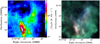 |
Fig. 4 Left: 0th moment of the 12CO(2–1) observationscarried out with the IRAM 30 m over the extended G region. This map corresponds to the signal integrated in the velocity interval [−40; +30] km s−1. The color scale used to represent data is logarithmic to enhance the dynamic range and emphasize the fainter molecular cloudlet. Right: composite image of our field of observations in the extended G region, using an IRAM 30 m data cube as well as Spitzer-MIPS data; 12CO(2–1) ([−40, +30] km s−1 as in the left panel) is coded in red, MIPS-24 μm in blue, and 13CO(1–0) [−4.0, −2.5] km s−1, corresponding to the emission spatially and kinematically associated with the ambient cloud described by Lee et al. (2012) in green. Color scale levels are based on the minimum and maximum value of each map. |
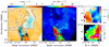 |
Fig. 5 Left: first moment map of the IRAM 30 m 12CO(2–1) data cube. Center: second moment map of the same data cube. Right, top panel: zoom into the dashed box on the first moment map of the APEX 12CO (3–2) data cube to enhance the spectral resolution. Right top and bottom panels: first and second moment maps of the APEX 12CO(3–2) data cube into the dashed box shown in the right and middle panels, respectively. The color bar of the left figure is centered on the velocity of IC443 in the local standard of rest, vLSR = −4.5 km s−1. |
4 Column density and mass measurements
4.1 Spatial separation of spectrally uniform structures
We aim to measure the mass associated with each molecular structures described in the previous section. We defined spatial boundaries enclosing these structures and independently studied the spectral data corresponding to each subregion of the field. The spatial boxes defined for the cloudlet (A), ring-like structure (B), shocked clump (C), and shocked knot (D) are shown in Fig. 6, and the average spectra obtained in these boxes are presented in Figs. 8 and 7 for every line from CO and its isotopologs, which are available in our IRAM 30 m and APEX data cubes. The choice of the boundaries is based on our morphological classification, but we carefully checked that the brightest spectral features are coherent across the different boxes that we defined (coordinates of these boxes are given in Table A.1). We performed that selection manually, as the size of our sample is not large enough to apply statistical methods (e.g., clustering, see Bron et al. 2018). Based on the analysis of the emission of 12CO, 13CO and C18O lines, our description of these spectral features is the following:
- 1.
Cloudlet: toward box A (Fig. 7, left-panel), the line profile of 12CO and 13CO lines are similarly double peaked and best modeled by the sum of two Gaussian functions centered on the systemic velocities vLSR = −5.7 ± 0.3 km s−1 (associated with the cloudlet) and vLSR = −3.3 ± 0.1 km s−1 (associated with the ambient cloud).
- 2.
Ring-like structure: toward box B (Fig. 7, right-panel), the 12CO and 13CO lines are double peaked as well. The use of two Gaussian functions to model the line profile yields the systemic velocities vLSR = −5.6 ± 0.2 km s−1 (associated with the ring-like structure) and vLSR = −3.3 ± 0.1 km s−1 (associated with the ambient cloud). The Gaussian decomposition is very similar to that of the cloudlet, suggesting that the apparent ring-like structure might be incidental despite its remarkable features in the first moment map (Fig. 5).
- 3.
Shocked clump: considering the geometry of the SNR and the locally perpendicular direction of propagation of the SNR shockwave (van Dishoeck et al. 1993), the high-velocity emission arises from at least two shock waves, if not a collection of transverse shocks propagating along the molecular shell. In other words, the projection along the line of sight of several distinct shocked knots with distinct systematic velocities could contribute to the broadening of the 12CO lines. We measure vs ≃ 27 km s−1 and vs ≃ 21 km s−1 for the blueshifted and redshifted transverse shocks, respectively. Except for the J = 1–0 spectrum for which the emission of the ambient gas contributes to the average spectra, all spectra of 12CO lines exhibit a significant absorption feature around the vLSR of IC443G, suggesting that there is strong self-absorption of the emission lines. Evidence of line absorption is found in the velocity range −6 km s−1 < vLSR < −2 km s−1, which is where we detect the spatially extended features associated with the NW-SE complex of molecular gas described by Lee et al. (2012). Hence, it is possible that the foreground cold molecular cloud is at the origin of the absorption of the 12CO J = 1–0 and J = 2–1 lines. A faint and thin emission line is detected around v = 6.5 km s−1 both in the 12CO and 13CO spectra. This signal is associated with the NE–SW complex of molecular gas described in Sect. 3.2.
- 4.
Shocked knot: the shock signature of this line is distinct from the shocked clump. As hinted by the moments map (Fig. 5), its fainter high-velocity wings are displaced toward negative velocities. A self-absorption feature is also observed in this structure. Between v = −5.5 km s−1 and v = −2 km s−1 a bright andthin feature traces the ambient gas shown on the channel maps in Fig. 2 (second row from bottom; first, second and third panels from left).
The line width measured from the 13CO line profiles when we consider only the spectral component that are physically associated with the cloudletand ring-like structure (discarding the contribution of the ambient cloud) are 2.0 ± 0.3 km s−1 and 1.6 ± 0.3 km s−1, respectively,measured by carefully defining much more constrained spatial boundaries around the structures. From the average spectra presented in this section, there is no spectral evidence for the propagation of molecular shocks and/or outflows within these two structures, except for the faint wings displayed by the 12CO lines in the box associated with the ring-like structure. These extended wings arise from the contamination by the high-velocity emission of the shocked substructures that are contained in box B (Fig. 5). We measured the peak temperature, velocity centroid, FWHM, and area of the 12CO and 13CO lines J = 1–0, J = 2–1 and J = 3–2 in each average spectrum and report our results in Table 3.
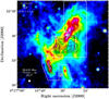 |
Fig. 6 Spitzer/MIPS map at 24.0 μm. In black contours, the emission of 12CO(2–1) observedwith the IRAM 30 m is shown over different intervals of velocities: A [−7; −5] km s−1 (cloudlet); B[−5.5; −4.5] km s−1 (ring-like structure); and C and D [−40; +30] km s−1 (shocked clump and shocked knot). The white boxes represent the area where the signal corresponding to each structure is integrated. The beam diameter of the IRAM 30 m observations of 12CO(2–1) is shown in the bottom left corner. |
4.2 LTE method
4.2.1 Two-dimensional histograms of CO data
In the next section, we aim to build population diagrams in which we correct the effect of optical depth on the column density of upper levels. To measure the optical depth of CO lines, we relied on several strong assumptions, in particular the adopted isotopic ratios and the identity of excitation temperature for 12CO and 13CO (see Sect. 4.2.2 for a description of our method, and Roueff et al. 2020 for a complete discussion of the corresponding assumptions). To assess the validity of this approach and estimate the key parameters (isotopic ratios and excitation temperature ratios), we built 2D histograms from the 12CO J = 1–0, J = 2–1, J = 3–2 data cubes, as well as 13CO and C18O J = 1–0 data cubes to compare the line intensity from different isotopologs and rotational transitions of CO with modified LTE models (Bron et al. 2018). These assumptions are also discussed in Sect. 4.2.3. We examined four different 2D data histograms:
- 1.
J = 1–0 line intensity, 13CO vs. 12CO.
- 2.
J = 1–0 line intensity, 13CO vs. C18O.
- 3.
J = 1–0 line intensity ratio, [13CO/C18O] vs. [12CO/13CO].
- 4.
12CO line intensity ratio, [3–2]/[2–1] vs. [2–1]/[1–0].
In order to build the first three data histograms, we convolved all IRAM 30 m data cubes to the nominal spatial resolution of C18O(1–0) (i.e., 23.6′′) and to the nominal spectral resolution of the FTS backend (i.e., 0.5 km s−1). To build the fourth histogram, we resampled IRAM 30 m 12CO(1–0), APEX 12CO(2–1), and APEX 12CO(3–2) data cubes to the nominal spatial resolution of 12CO(1–0) (i.e., 22.5′′) and to the nominal spectral resolution given by the FTS backend (i.e., 0.5 km s−1). We used a threshold of 3σ to select data points for which the signal is significantly above the noise level. The resulting 2D data histograms are shown in Fig. 9.
Results
The first histogram is characterized by a high (S/N) ratio and represents a large statistical sample (n = 20 531). The 13CO(1–0) vs. 12CO(1–0) relation presents at least two distinct branches. The lower quasi-horizontal branch, tracing bright 12CO(1–0) emission associated with faint 13CO(1–0) line emission (T13 < 1 K km s−1). This branch is spatially correlated with the shock structure and spectrally correlated with the high-velocity wings of the 12CO line, which have no bright 13CO counterpart because of insufficient integration time. It is spatially correlated mainly with the quiescent molecular gas that is found within the cloudlet and ring-like structure and the ambient cloud.
The 13CO(1–0) vs. C18O(1–0) histogram has a much smaller number of bins determined with a good (S/N) (n = 833) due to the faint emission of C18O(1–0) that is hardly detected at a 3σ confidence level within our data cube. Still, we find evidence of at least one statistically significant branch. As a result of to the small size of the sample, it is not possible to identify any spatial or spectral correlation with certainty.
The third histogram has a poor statistical sample for the same reason as the second one (n = 833). The [13CO(1–0)]/ [C18O(1–0)] ratio vs. [12CO(1–0)]/[13CO(1–0)] relationship is localized in an area with little dispersion. Hence, for high signal-to-noise measurements the isotopic ratios are almost uniform in the field of observations. Nonetheless, the lower signal-to-noise data bins display a statistically well-defined comet-shaped branch extending from this area. This branch might correspond to distinct physical conditions and/or isotopic ratios for a fraction of the field of observations. The high (S/N) area of this branch is spatially correlated with the cloudlet and ring-like structure, whereas the “tail” of the branch is spatially and spectrally associated with the shocked clump.
The fourth histogram is built on a large statistical sample with high signal-to-noise data (n = 9793), as the rotational lines J = 1–0, J = 2–1, and J = 3–2 are well detected in our data cubes. The 12CO [3–2]/[2–1] vs. [2–1]/[1–0] relationship is clearly bimodal. A quasi-vertical branch centered on [2–1]/[1–0] ≃ 0.5 can be distinguished from a crescent-shaped branch centered on [2–1]/[1–0] ≃2 and [3–2]/[2–1] ≃1.3. The crescent-shaped branch is highly correlated to the high-velocity wings of the 12CO lines tracing the emission of shocked gas, where it is expected to measure high, enhanced J = 2–1 / J = 1–0 ratio (e.g., Seta et al. 1998).
We compared the observational histograms with synthetic families of curves generated using modified LTE radiative transfer models of the observed rotational transition for 12CO, 13CO, and C18O. Assuming that CO is at thermal equilibrium, the intensity of the line integrated over an element of spectral resolution (Δv = 0.5 km s−1) is given by
 (1)
(1)
where α = 12, 13, 18 (histograms 1–3) or α = 1–0, 2–1, 3–2 (histogram 4) for the 12CO, 13CO, C18O isotopologs, respectively,and J = 1–0, J = 2–1, J = 3–2 rotational lines. The quantity Tα is the integrated intensity of the line, defined as
 (2)
(2)
where  is the temperature of the transition or energy of the upper level Eup, given in Table 1 for all studied lines; τα is the optical depth of the line; Tcmb is the cosmic microwave background temperature; and
  is the excitation temperature of the line. The optical depth τα and its dependence on the excitation temperature is described by
 (3)
(3)
where  is the optical depth at a kinetic temperature T0. We used the optical depth at T0 = 20 K as a reference. We made the assumption that the excitation temperature of the different isotopologs (
 ,
,  ,
,  ) and rotational lines (
 ,
,  ,
,  ) are distinct and controlled their ratios as four supplementary independent parameters of the modified LTE models (Roueff et al. 2020). The opacities of 12CO and C18O isotopologs were determined from the optical depth of 13CO using the corresponding isotopic ratio as follows:
![Mathematical equation: \begin{equation*} \dfrac{\tau_{12}}{\tau_{13}}\,{=}\,\dfrac{[^{12}\mathrm{CO}]}{[^{13}\mathrm{CO}]},~\dfrac{\tau_{13}}{\tau_{18}}\,{=}\,\dfrac{[^{13}\mathrm{CO}]}{[\mathrm{C^{18}O}]} .\end{equation*}](/articles/aa/full_html/2020/12/aa38339-20/aa38339-20-eq15.png) (4)
(4)
Lastly, we assumed a hierarchy in the optical depth of the different rotational lines such that τ1−0 ≥ τ2−1 ≥ τ3−2 and control their ratio as two supplementary parameters of the modified LTE models (Roueff et al. 2020). Hence, there are a total of nine control parameters that we can set: the optical depth τ13, isotopic ratio ![Mathematical equation: $[^{12}\mathrm{CO}] / [^{13}\mathrm{CO}]$](/articles/aa/full_html/2020/12/aa38339-20/aa38339-20-eq16.png) , isotopic ratio
, isotopic ratio ![Mathematical equation: $[^{13}\mathrm{CO}] / [\mathrm{C^{18}O}]$](/articles/aa/full_html/2020/12/aa38339-20/aa38339-20-eq17.png) , temperature ratios [
, temperature ratios [ /
/ ], [
], [ /
/ ], [T3−2/T2−1], [T2−1/T1−0], and optical depth ratios [τ3−2/τ2−1], [τ2−1/τ1−0]. We used the kinetic temperature of 13CO as a variable of the parametric equation
  to synthesize LTE models that we can plot on top of each 2D data histogram. Each curve in Fig. 9 corresponds to a given set of control parameters, with the kinetic temperature growing linearly along a curve. We produced a family of LTE models with linearly increasing optical depth and a kinetic temperature varying between 10 and 25 K, corresponding to the typical temperatures of cold molecular clouds. We adopted the isotopic ratio
 ![Mathematical equation: $[^{12}\mathrm{CO}] / [^{13}\mathrm{CO}]$](/articles/aa/full_html/2020/12/aa38339-20/aa38339-20-eq23.png) and
and ![Mathematical equation: $[^{13}\mathrm{CO}] / [\mathrm{C^{18}O}]$](/articles/aa/full_html/2020/12/aa38339-20/aa38339-20-eq24.png) that offers the best visual match with our data, and similarly fine-tuned the other control parameters to reproduce the branches observed in each 2D data histogram.
that offers the best visual match with our data, and similarly fine-tuned the other control parameters to reproduce the branches observed in each 2D data histogram.
All other parameters remaining constants, each control parameter has an effect on the pattern and location of a curve in the histogram space:
An increase in the isotopic ratio
![Mathematical equation: $[^{12}\mathrm{CO}] / [^{13}\mathrm{CO}]$](/articles/aa/full_html/2020/12/aa38339-20/aa38339-20-eq25.png) translates the curves downward in the histogram 1, does not modify the histogram 2, and translates the curves rightward in the histogram 3.
translates the curves downward in the histogram 1, does not modify the histogram 2, and translates the curves rightward in the histogram 3.An increase in the isotopic ratio
![Mathematical equation: $[^{13}\mathrm{CO}] / [\mathrm{C^{18}O}]$](/articles/aa/full_html/2020/12/aa38339-20/aa38339-20-eq26.png) does not modify the histogram 1, translates the curves upward in the histogram 2, and translates the curves upward in the histogram 3.
does not modify the histogram 1, translates the curves upward in the histogram 2, and translates the curves upward in the histogram 3.The modification of the temperature ratios alters the shape and orientation of the curves in histograms 3 and 4, and determines the boundaries of the 12CO and C18O curves.
The LTE models that visually best match our data are represented in Fig. 9 over the data histograms, and their corresponding set of control parameters are summarized in Table 4. A kinetic temperature in the range 10–25 K is sufficient to account for most of the data where the sample is statistically significant, and we did not need to assume that [ /
/ ] and [
 /
/ ] are different from 1 to find a satisfactory fit. However, to obtain a model that accounts for the high [3–2]/[2–1] and [2–1]/[1–0] data bins (histogram 4), it was necessary to set their temperature ratios as greater than 1, such that we inferred an average temperature of up to ~55 K traced by the J = 2–1 lines, and up to ~120 K for the J = 3–2 lines in the high-velocity wings. This area of the histogram 4 also required lower τ2−1∕τ1−0 and τ3−2∕τ1−0 ratios, that we set to 0.2 for our models, suggesting that optical depth decreases significantly in the high-velocity wings of the lines. Considering histogram 3, our best models indicate a value of the isotopic ratio
 ![Mathematical equation: $[^{12}\mathrm{CO}] / [^{13}\mathrm{CO}]\,{=}\,45$](/articles/aa/full_html/2020/12/aa38339-20/aa38339-20-eq31.png) –90 and
–90 and ![Mathematical equation: $[^{13}\mathrm{CO}] / [\mathrm{C^{18}O}]\,{=}\,20$](/articles/aa/full_html/2020/12/aa38339-20/aa38339-20-eq32.png) –45 to account for the emission of the different isotopologs observed in the extended G field. A large range of isotopic ratios can account for the observed data spread in histogram 3, hence this result does not provide a precise determination of the
–45 to account for the emission of the different isotopologs observed in the extended G field. A large range of isotopic ratios can account for the observed data spread in histogram 3, hence this result does not provide a precise determination of the ![Mathematical equation: $[^{12}\mathrm{CO}] / [^{13}\mathrm{CO}]$](/articles/aa/full_html/2020/12/aa38339-20/aa38339-20-eq33.png) and
and ![Mathematical equation: $[^{13}\mathrm{CO}] / [\mathrm{C^{18}O}]$](/articles/aa/full_html/2020/12/aa38339-20/aa38339-20-eq34.png) abundances. The higher boundary of our 12C/13C ratio estimate is anomalous with respect to the local ISM average of 62 ± 4 (Langer & Penzias 1993), however Wilson & Rood (1994) provide an estimate of the elemental abundances based on their distance to the Galactic center (GC):
abundances. The higher boundary of our 12C/13C ratio estimate is anomalous with respect to the local ISM average of 62 ± 4 (Langer & Penzias 1993), however Wilson & Rood (1994) provide an estimate of the elemental abundances based on their distance to the Galactic center (GC):
 (5)
(5)
If we adopt the distance of 1.9 kpc for IC443 (Ambrocio-Cruz et al. 2017) the SNR is located at a distance of ~10 kpc from the GC. Hence our estimate of the 12CO∕13CO ratio is in agreement with the expected abundance of 80 ± 30, but our measured 13CO∕C18O is much higher than the predicted ratio of 8 ± 2. The measured enhancement of the 13CO∕C18O ratio might be the product of the fractionation of carbon monoxide by photodissociation, as the shielding of the various isotopologs of CO provides a mechanism for the rarefaction of C18O with respectto the expected abundance (e.g., Glassgold et al. 1985). We checked the spatial distribution of data points corresponding to particular areas of the histograms presented in Fig. 9.
Histogram 3: interestingly, the data points corresponding to high (> 20) 13CO∕C18O line ratio are spatially correlated with the cloudlet only. If no protostars are positively identified toward the cloudlet (Sect. 5), radiative decay from X-ray irradiation seen in the SNR cavity with XMM-Newton might provide a source to account for the selective photodissociation of CO within the cloudlet (Troja et al. 2006; Troja et al. 2008).
Histogram 4: data points corresponding to high (>2) [J = 2 − 1]∕[J = 1−0] and [J = 3−2]∕[J = 2−1] ratios are spatially correlated with the shocked clump, and spectrally correlated with the high-velocity wings of themolecular line. The most striking spatial correlation is seen toward the eastern surface layer of the shocked clump, where the molecular gas seems to be systematically characterized by a large (> 2) [J = 3−2]∕[J = 2−1] and small (<1) [J = 2−1]∕[J = 1−0] ratio apparently tracing the shock front. However, this combination of line ratios is not predicted by RADEX models and could be due to an inaccurate registration between the data sets.
 |
Fig. 7 Spectra averaged over the regions of the cloudlet (left panels) and the ring (right panels) defined in Fig. 6 for the following lines: 12CO (1–0), 13CO (1–0) and C18O(1–0) (in black, IRAM-30m); 12CO(2–1), 13CO (2–1) and C18O(2–1) (in blue, APEX); 12CO(3–2) and 13CO(3–2) (in grey, APEX). Spectral cubes were resampled to allow a direct comparison between the different spectra. Spatial resolutions of all transitions were modified to the nominal resolution of C18O (2–1), θ = 30.2′′. Spectral resolutions were set to 0.5 km s−1 for IRAM 30m data and 0.25 km s−1 for APEX data. On both panels, the vLSR of IC443 is indicated with a vertical dashed line (at − 4.5 km s−1). |
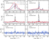 |
Fig. 8 Spectra averaged over the region of the shocked clump (left) and shocked knot (right) defined in Fig. 6 for the following lines: 12CO (1–0), 13CO (1–0) and C18O(1–0) (in black, IRAM 30 m); 12CO(2–1), 13CO (2–1) and C18O(2–1) (in blue, APEX); 12CO(3–2) and 13CO(3–2) (in grey, APEX). Spectral cubes were resampled to allow a direct comparison between the different spectra. Spatial resolutions of all transitions were modified to the nominal resolution of C18O (2–1), θ = 30.2′′. Spectral resolutions were set to 0.5 km s−1 for IRAM 30m data and 0.25 km s−1 for APEX data. On both panels, the vLSR of IC443 is indicated with a vertical dashed line (at − 4.5 km s−1). |
 |
Fig. 9 Data histograms and LTE models of the emission of the rotational transitions of 12CO and its isotopologs mapped in the extended G field with the IRAM 30 m and APEX: 1. 13CO (1–0) vs. 12CO(1–0); 2. 13CO (1–0) vs. C18O(1–0); 3. [13CO(1–0)] / [C18O (1–0)] vs. [12CO(1–0)] / [13CO (1–0)]; and 4. 12CO(3–2) / 12CO (2–1) vs. 12CO(2–1) / 12CO (1–0). The color map corresponds to the amount of data points (line of sight and velocity channels) that fall into a given bin of the histogram. The curves represent families of models of the LTE intensity as a function of the kinetic temperature of 13CO. The arrows indicate the direction in which the kinetic temperature grows along a given curve. Control parameters of the LTEmodels are given in Table 4 for each histogram. The dashed black lines represent the 3σ detection level for each axis (histograms 1 and 2). |
4.2.2 Population diagrams
We determined the physical conditions (column density NCO, and kinetic temperatureTkin) of the molecular gas in the extended G region assuming that the emission lines are thermalized. We used pixel-per-pixel population diagrams (Goldsmith & Langer 1999) corrected for optical depth for the 12CO(3–2), 12CO(2–1), and 12CO(1–0) transitions to measure the upper level column density Nup (hereafter level population) for Jup = 3, Jup = 2, Jup = 1. Systematically, the 13CO data is usedto correct the effect of optical depth in the population diagrams, for each element of resolution (i.e., for each of line of sight), and for all velocity channels. To perform this task we chose to use the APEX data cube over the IRAM 30 m data cube to measure the specific intensity corresponding to the 12CO(2–1) transition. The IRAM 30 m has the advantage of having lower noise (see Table 2). However, the 13CO(2–1) transition was only observed with the APEX telescope owing to receiver setup constraints. Hence to avoid intercalibration issues, we used the APEX data for 12CO(2–1) and 13CO(2–1). First, we convolved all maps to the same spatial resolution for consistency, using the nominal resolution of 13CO(2–1), such that we have a beamdiameter of 30.1′′ for the six maps considered. The spectral resolution was also modified and set to 2 km s−1 for each transition to increase the S/N. Then, the following measurements were performed pixel-per-pixel using a Python5 algorithm:
- 1.
Sigma-clipping was applied to the spectra of all transitions of the two isotopologs 12CO and 13CO, using a threshold of 3σ.
- 2.
In every single velocity channel remaining after sigma-clipping, the NJ = 3, NJ = 2, and NJ = 1 level populations were measured both for 12CO and 13CO to determine the optical depth of the three transitions using the adopted value of isotopic ratio. We measured the optical depths τ3−2, τ2−1 and τ1−0, assuming that 13CO lines are optically thin and that the excitation temperatures of the two isotopologs are approximately equal (this second assumption is supported by the results presented in Sect. 9). Under this assumption we have
 (6)
(6)
 (7)
(7)where βij = [1 −e−τij]∕τij is the escape probability of a photon, νij the frequency of the transition, Nup the level population, Aij the probability of the transition, and Iν the specific intensity. Based on the comparison of our data with modified LTE models (Sect. 4.2.1) we adopted different values for the expected isotopic ratio toward each region (indicated in Table 5).
- 3.
The estimates of 12CO level populations were corrected for optical depth using the correction factor
 , such that the corrected column density is given by
  .
. - 4.
We put the corrected level populations
 and their corresponding energies Eup = hνij∕kB into the population diagram
  and used a χ2-minimization algorithm6 to determine the best linear fit y = ax + b. The excitation temperature Tex is deduced from the slope, and the total column density NCO is determined by computing the partition function Q(Tex)7 and measuring the offset.
 - 5.
We finally derived the mass of the gas from the measured total column density NCO, using the expected
![Mathematical equation: $[\mathrm{H_2}] / [^{12}\mathrm{CO}]$](/articles/aa/full_html/2020/12/aa38339-20/aa38339-20-eq42.png) ratio toward dense molecular regions and assuming that the distance of IC443 is 1.9 kpc (Ambrocio-Cruz et al. 2017). We adopted the value of 104 for the H2 -to-12CO abundance ratio (Gordon & Burton 1976; Frerking et al. 1982), thus we have
ratio toward dense molecular regions and assuming that the distance of IC443 is 1.9 kpc (Ambrocio-Cruz et al. 2017). We adopted the value of 104 for the H2 -to-12CO abundance ratio (Gordon & Burton 1976; Frerking et al. 1982), thus we have  , where
  is the area of the box and mH the mass of hydrogen.
Results of the population diagrams analysis for each structure.
Uncertainties
The error bars on total CO column density, gas mass, and kinetic temperature are determined by the following: (i) instrumental errors, dominated by the systematic uncertainty on the flux (Sect. 3.1.3); (ii) the quality of the linear fit applied to the population diagram; and (iii) systematic errors on the adopted distance of IC443 and the 12CO/13CO isotopic ratio.
Results
Average population diagrams are presented in Figs. 10 and 11, based on the spatial boxes defined in Fig. 6 and integration ranges defined in Table 6. The measurements obtained are presented inTable 5, in which the minimum and maximum boundaries are given for the total CO column density, gas mass, and kinetic temperature. We measured the column densities and masses for the regions A (cloudlet), B (ring-like structure), C (shocked clump), and D (shocked knot) as indicated in Fig. 6, and also for the ambient cloud by averaging the signal over the entire field (regions A, B, C and D excluded). We also measured the mass of the foreground clump that spatially coincides with the shocked clump using a Gaussian model for the average CO lines in the velocity range [2.5; 12] km s−1. The result of this measurement is presented at the end of Table 5.
4.2.3 Discussion
As a first-order verification we compared our measurement of the mass based on the population diagram with a rough estimate of the mass using the CO(J = 1–0)-to-H2 conversion factor XCO (Dame et al. 2001; Bolatto et al. 2013). We adopted the following conversion factor, with a ± 30% uncertainty, which is written as
 (8)
(8)
The H2 column density was determined by the product of XCO with the area of the raw 12CO J = 1–0 line (without optical depth correction), and the mass was inferred from  in the same manner as described previously. We report the results of this measurement in the last column of Table 5, referred to as
  . Within error bars, almost all our measurements are consistent with this rough estimate of the mass, except for the line wings toward the shocked clump. With respect to the population diagram method, this method systematically overestimates the mass. The enhanced J = 2–1/J = 1–0 emission of the high-velocity gas accounts for a lower mass in the population diagram, as it traces a warmer gas for which the XCO conversion factor yields an overestimate.
We built a single population diagram for each spatial box, using a single value of Nup that is the spatial and spectral average of our sample of measurements. The resulting population diagrams are shown in Fig. 10; statistical information on the spread of the sample around these average values of Nup is also represented. As additional information on the thermalization of carbon monoxide, in Fig. 11 we show the average population diagrams obtained using the 13CO lines with the same method, without correction of the optical depth.
- 1.
Thermalization: at a temperature of 10 K, the critical density nij = Aij∕Cij of the 12CO J = 1–0, J = 2–1 and J = 3–2 lines are n1−0 = 2.2 × 103 cm−3, n2−1 = 2.3 × 104 cm−3, respectively, and n3−2 = 3.5 × 104 cm−38. Toward the shocked clump, it is likely that these critical densities are attained (Cesarsky et al. 1999), hence the lines should be thermalized. In the population diagrams shown in Fig. 10, the average data points are generally in satisfactory agreement with the assumption that the emission lines are thermalized, as there is no significant divergence from the Boltzmann distribution for any of the structure studied. The highest value of χ2 is obtained toward the ambient cloud, which also presents an abnormally low kinetic temperature, down to ~5 K. This might indicate that the J = 2–1 and J = 3–2 are sub-thermal, which is expected if some parts of the NW-SE molecular cloud we are probing have a density lower than 104 cm−3. There is a systematic discrepancy between the linear fit and the measured column density of the upper level J = 2, which is lower than expected in each structure. This anomaly can be solved if we adopt two distinct kinetic temperatures to model the relative distribution of the level populations. In the high-velocity wings of the lines, it is expected and it was hinted by our LTE analysis (Sect. 4.2.1) that the J = 2–1 and J = 3–2 lines trace a warmer gas than theJ = 1–0 line that is primarily tracing the quiescent and cold phase. In this case, the distribution in these population diagrams should be modeled by a linear fit of kinetic temperature T1 for the upper levels Jup = 1,2 (cold component) and a linear fit of temperature T2 for levels Jup = 2,3 (warm component), hence assuming that along a line of sight we observe two layer of gas thermalized at distinct temperatures, where T1 < T2. In Table 5 we present the temperature obtained for the warm component as well as the mass of the cold component. The statistical spread of our sample of measured level populations around the average linear distribution provides a strong motive for the use of pixel-per-pixel, channel-per-channel population diagrams, as it is evidence of a large range of physical conditions that require distinct LTE models.
- 2.
Filling factor: the filling factor used to infer column densities from the main beam temperature measured during our observations is set to 1. From the morphology of the gas mapped in 12CO(2–1) with the IRAM 30 m with a nominal resolution of 11.2′′ (Figs. 4, 2) we consider that we are probing extended, clumpy structures with dimensions that are greater than the beam diameter characterizing our observations, between and 19.2′′ and 30.1′′ for the data cubes used to measure the gas mass.
- 3.
Optical depth: the measurement of the optical depth from the comparison of the fluxes between 12CO and 13CO is shown in the appendix along with the measurement based on the 12CO/C18O isotopic ratio (Fig. F.1). The optical depth is non-negligible both in the ring-like structure and cloudlet. It is important in the self-absorbed component of the emission lines corresponding to the shocked clump where the cold, ambient cloud intervenes, and much lower in the high-velocity wings. We checked the assumption that 13CO is optically thin using the C18O J = 1–0 and J = 2–1 lines to estimate its optical depth based on the expected 13CO/C18O isotopic ratio. In our pixel-per-pixel, channel-per-channel population diagrams the correction of the optical depth is partially biased, as the detection of 13CO is limited by the noise level. At a certainty level of 5σ, we cannot measure a flux lower than 125, 420, and 400 mK for the J = 1–0, J = 2–1, and J = 3–2 transitions, respectively. As a consequence, toward a significant number of lines of sight and velocity channels the optical depth is measured for the J = 1–0 transition but not for J = 2–1 and J = 3–2. In the population diagram this results in the biased displacement of the level J = 1 with respect to the levels J = 2 and J = 3, hence the slope of the linear fit is artificially enhanced and the excitation temperature is lowered (Fig. 10, Table 5).
- 4.
Self-absorption of CO lines toward the shocked clump: we performed an independent measure of the temperature and column density of the absorbing envelope of the shocked clump from the absorption features of CO lines. Toward the position (6h 16m42.5s, + 22°32′12′′), we renormalized the signal in each frequency channel with respect to the profile of the emission lines and measured the optical depth for all transitions in a beam of radius 22.5′′. From the equivalent widths W of the transitions J = 1–2 and J = 0–1, we measured the temperature of the gas solving the following equation:
 (9)
(9)where T0 = hν∕k and F(u) = e−3ucosh(u) (see Appendix B). We obtained an excitation temperature of 18 ± 3K. We then built a population diagram of the lower population Nl levels from the measures of the optical depth, using the following relation:
 (10)
(10)where ful is the oscillator force, λ the wavelength of the transition, and σv the velocity dispersion of the absorbing medium, which we assume to be equal to the velocity dispersion of the lines associated with the shocked clump that we measured in Table 3. This population diagram yields a total column density of the absorbing medium NCO = 3.4 × 1016 cm−2, corresponding to a total mass of 20 M⊙ for the absorbing envelope of the shocked clump.
 |
Fig. 10 Average population diagrams of 12CO corrected for optical depth. The measured average, first quartile, third quartile, fifth percentile, and 95th percentile associated with our sample of level populations corresponding to Jup = 1, Jup = 2, and Jup = 3 are indicated for two adopted values of the 12CO/13CO isotopic ratio (12CO/13CO = 60 in black, 12CO/13CO = 100 in red). The black solid line represents the linear fit of the black data points. The boundaries of the filled areas are defined by the linear fits corresponding to the first and third quartiles for each value of the isotopic ratio adopted. The 5th percentile and 95th percentile are indicated by the caps, the first quartile and third quartile are indicated by the ends of the box, and the average is indicated by the cap inside of the box. Each diagram accounts for a sample of measurements performed in one of the spatial boxes defined in Fig. 6 and integration ranges defined in Table 6: (a) the shocked clump, (b) the cloudlet, (c) the ring, (d) the ambient cloud, and (e) the shocked knot. |
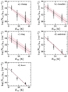 |
Fig. 11 Average population diagrams of 13CO. The measured average, first quartile, third quartile, 5th percentile, and 95th percentile associated with our sample of measured level populations are indicated for each level. The black solid line represents the linear fit of the average data points. The boundaries of the filled areas are defined by the linear fits corresponding to the first and third quartiles. Each diagram accounts for a sample of measurements performed in one of the spatial boxes, as in Fig. 10. |
4.3 LVG method
The results obtained in the previous section are based on several strong assumptions, in particular that the excitation temperature of 12CO and 13CO are equal. To address this issue, we investigated the application of a second method that does not require this assumption to determine the mass of the gas toward our field of observations using CO lines. We used the LVG model for an expanding spherical shell (e.g., Sobolev 1960, Surdej 1977) to model the lines observed. This model requires a local, LVG ∇v along the line of sight. We consider that this assumption is verified throughout the field of observation as the line width of 12CO lines suggests typical turbulent broadening (Sect. 3.3). We used the non-LTE radiative transfer RADEX code (van der Tak et al. 2007), a computer program that solves the radiative transfer equation based on the escape probability formulation in an isothermal and homogeneous medium characterized by a LVG. Three geometries are available. We selected the expanding spherical shell for which the escape probability is related to the optical depth τ by the following formula (Mihalas 1978):
 (11)
(11)
In the framework of the LVG assumption, the value of the optical depth at line center determined by RADEX is proportional to N/Δv, where N is the column density and Δv the full width at half-maximum of the line profile. Hence when using RADEX the choice of the parameter Δv is critical to model the expected intensities of atomic and molecular lines. The program solves the statistical equilibrium equations taking into account up to seven collisional partners, allowing us to analyze spectral line observations if the molecular collisional data is known. RADEX models require a total of seven input parameters: the column density N, local density  , kinetic temperature Tkin, line width Δv, and background temperature Tb. In return, RADEX estimates the excitation temperature Tex, optical depth τij, peak temperature TR, upper and lower level populations Nup, Nlow, and flux ∫ Tdv of an arbitrary number of transitions defined by the user.
We applied the LVG method to average spectra measured over the extent of each box defined in Fig. 6 and velocity ranges defined in Table 6. Using a χ2 minimization, we compared RADEX outputs with our measurements to constrain the physical conditions. We compared the line intensities of the three first rotational transitions of 12CO and 13CO with a grid of RADEX models. In the same manner as in the population diagram approach, for consistency we convolved all maps to the same spatial resolution, using the nominal resolution of 13CO(2–1), such that we have a beam diameter of 30.1′′ for the six maps considered. The spectral resolution was also set to 2 km s−1 for each transition to increase the S/N. Then we produced several 3D grids of RADEX models with the varying parameters (N,  , T) and fixed parameters (Tb, Δv). These parameters are specified in Table 7 for the different grids used. We used large ranges of column densities and kinetic temperature to probe a consistent fraction of the space of parameters, corresponding to a variety of physical conditions as wide as possible. We set the value of the parameter Δv based on the equivalent linewidth that we measured on average spectra using bi-Gaussian functions to model the line profiles. We took the following steps for each average spectrum using a Python algorithm:
- 1.
We applied sigma-clipping to the spectra of all transitions of 12CO and 13CO, using a threshold of 3σ.
- 2.
We measured the specific intensity of each transition on the velocity range corresponding to each spectral feature (e.g., the wings of the shocked clump are treated separately from the core of the line). Then, in each element of the model grid we computed the following quantity, corresponding to a combined reduced χ2 statistical estimator:
![Mathematical equation: \begin{equation*}\chi^2_{\mathrm{RADEX}}\,{=}\,\dfrac{1}{2} \sum\limits_{J_{\mathrm{up}}\,{=}\,1}^{3} \left[ \dfrac{\left(s_{12}^{\mathrm{RADEX}} - s_{12}^{\mathrm{obs}}\right)^2}{3 \sigma\left(s_{12}^{\mathrm{obs}}\right)^{2}} + \dfrac{\left(s_{13}^{\mathrm{RADEX}} - s_{13}^{\mathrm{obs}}\right)^2}{3 \sigma\left(s_{13}^{\mathrm{obs}}\right)^{2}} \right] .\end{equation*}](/articles/aa/full_html/2020/12/aa38339-20/aa38339-20-eq53.png) (12)
(12)In this equation, Jup indicates the upper levels of each transition,
 and
and  are respectively the specific intensity of 12CO and 13CO returned by a given RADEX model, sobs the observational intensity, and σ the uncertainty associated with the measurements of the intensity s.
 - 3.
The physical conditions for each average spectrum were deduced from the minimization of the quantity χ2, that is, we localized the minimum element of the resulting
 grid and inferred the quantities (N,
  , T) from the corresponding RADEX input.
The error bars on column density and kinetic temperature were estimated from the uncertainties on the flux and more importantly from the uncertainty on the isotopic ratio 12CO/13CO.
Summary of the results and parameters used in the LVG analysis.
Results
The results of our LVG analysis are presented in Table 7, in which the minimum and maximum boundaries are given for the CO column density and gas mass for the shocked clump, shocked knot, ring-like structure, cloudlet, and ambient cloud. As previously, we measured the molecular mass assuming that the H2 -to-12CO abundance ratio is equal to 104. The χ2 minimization was successfully attempted for the major part of our analysis. We present the χ2 diagrams for each region in Fig. 12, where the first and second term of Eq. (12) are independently represented by two sets of filled contours. For most structures, we were not able to determine a precise measurement of the local density from the χ2 minimization, as the variation of χ2 with respect to the choiceof the input  does not strongly favor any LVG model. In all cases we observe that χ2 increases significantly for densities
  cm−3, hence our analysis suggests that (i) the 12CO lines are thermalized; (ii) the local density is greater than 104 cm−3 across the field of observations.
4.4 Discussion
The gas masses measured with the LVG approach are systematically lower than the masses obtained using population diagrams corrected for optical depth (Table 5), except for the high-velocity wings for which the LVG estimate is higher by a factor ~3 and for the cloudlet for which both methods yield the same result. Deviation from a single excitation temperature is not sufficient to account for this discrepancy, since the LVG models that fit our data do not predict a disagreement higher than ~1 K for the excitation temperatures of 12CO and 13CO. This discrepancy is mainly due to the fact that the LVG method is applied to average spectra, whereas the LTE approach is applied pixel per pixel and channel per channel. The channel-per-channel measures of optical depth are particularly different from the average measures toward the shocked clump for which the optical depth varies strongly between thecenter of the line and high-velocity wings. The highest estimates of the mass are obtained using the CO-to-H2 conversion factor based on theemission of 12CO J = 1–0 only. In comparison to previous measures of the molecular mass in the extended G region:
Dickman et al. (1992) measured a mass of 41.6 M⊙ for the clump G assuming that 12CO J = 1–0 emission is optically thin.
Using a CO-to-H2 conversion factor, Lee et al. (2012) measured a mass of 57.7 ± 0.9 M⊙ for the cloudlet.
Xu et al. (2011) measured a mass of 2.06 × 10³ M⊙ for cloud G from the 12CO J = 3–2 line. Their measure included a larger field, and they lacked sufficient data to correctly estimate the optical depth.
Our new measurements of the mass are crucial for the interpretation of the interaction of CRs with the ISM. The extended G region is likely to be the main target of interaction with CRs, hence the source of teraelectronvolt γ-ray emission in IC443. Our results put constraints on the amount of molecular mass that is available to interact via bremsstrahlung and pion decay mechanisms. Torres et al. (2010) showed that the characteristics of the γ-ray spectra in IC443 suggest the interaction with two distinct molecular structures: a lower-mass cloud (~350 M⊙) at distance of 4 pc from the SNR and a higher-mass cloud (~4000 M⊙) at a distance of 10 pc. Their results were obtained from the analysis of the γ-ray spectra of the SNR in a larger field, yet they are consistent with our findings if we consider that the mass of the ambient gas that we measured could contribute to the distant component. As has been suggested by Lee et al. (2012), either the shocked clump or cloudlet and ring-like structure could correspond to the closer component, while the distant component might correspond to the ambient cloud. Within error bars, the mass we measured for these structures could fit with this scenario.
 |
Fig. 12 Diagrams of χ2 minimization of the comparison between 1 × 200 × 200 LVG grids modeled with sets of parameters ( |

![Mathematical equation: $\mathrm{log_{10}}(\chi^2_{\mathrm{RADEX}}) \leq [0.5, 0.45, 0.45, 0.5, 0.75, 0.75, 0.5]$](/articles/aa/full_html/2020/12/aa38339-20/aa38339-20-eq78.png)
5 Protostar candidates
In order to characterize the local star formation over the extent of the molecular structures characterized in the previous section, we studied the distribution of optical, infrared, and near-infrared point sources in the extended G region. We aimed to check if these infrared point sources can be identified as protostars and if so, to constrain their evolutionary stage based on their infrared fluxes. Finally, we aimed to study their spatial distribution and their association with the molecular clumps found in the extended G region.
5.1 Origin of the data
Our field was fully observed both by 2MASS and WISE. 2MASS operates between 1.235 and 2.159 μm, and WISE between 3.4 and 22 μm. The exact photometric parameters for each band of 2MASS and WISE are given in Table 8.
To recover point sources from these two catalogs, we used the NASA/IPAC infrared science archive to obtain all entries in a 10 arcmin sized square box around the field center α[J2000] = 6h16m37.5s, δ[J2000] = + 22°35′00′′, corresponding to the same field that was mapped with IRAM 30 m and APEX. A total of 487 point sources in the 2MASS All-Sky Point Source Catalog (PSC) and 515 point sources in the AllWISE Source Catalog were found using this query within the extended G region. Both catalogs provide position coordinates and photometric measurements for each band and their uncertainties, and S/Ns, along with several flags specifying contamination by extended emission, quality of the point spread function (PSF) profile-fit, and other possible sources of bias.
5.2 Selection of relevant IR point sources
In order to reject false positives, we applied several selection criteria to our primary catalogs of point sources detected by 2MASS and WISE:
- 1.
We required a complete detection in the WISE bands W1, W2, and 2MASS bands J, H, and K (i.e., the measurement is not an upper limit).
- 2.
We selected only the sources characterized by a signal-to-noise ratio greater than 2 for the photometric bands W1, W2, W3, J, H, and K.
- 3.
We rejected the WISE point sources that were flagged for confusion and/or contamination of the photometric bands by image artifacts.
- 4.
We rejected the 2MASS point sources that were flagged for low quality photometric measurements.
After this selection, 214/515 point sources remain for the AllWISE Source Catalog and 328/487 for the 2MASS PSC. A total of 99 point sources were detected both by 2MASS and WISE. AllWISE point sources marked with a value of ext_flg flag different than “0” are indicated as extended sources. Either their morphology is not consistent with the PSF of any band or they are spatially associated with a known extended source of the 2MASS Extended Source Catalog (XSC). 2MASS point sources with gal_contam = 0 are also sources that fall within the elliptical profile of a known extended source. A search in the 2MASS XSC catalog shows that 17 extended sources are found in our 10′ × 10′ field. The shocked clump is particularly crowded, suggesting that the extended emission of bright knot of shocked material are detected by the survey in this area. The photometric measurements are likely to be contaminated by this extended emission, hence the identification of these sources as protostar candidates is uncertain. Nonetheless, we do not completely rule out these entries in the catalog since this extended emission might be produced by outflows.
Photometric parameters for each band of the telescopes WISE, 2MASS and Gaia.
5.3 Color–color filtering
In order to select only the point sources that could possibly be YSOs, we applied a color–color criteria to our near-infrared point source catalogs. To identify the nature of a protostar candidate detected by 2MASS, we compared the relative flux in the J, K, and H photometric bands. We used the following empirical color criteria (Xu et al. 2011) based on the idea that protostars have an infrared excess in the 1.235–2.159 μm range that determines their position in the JHK color–color space and that is directly related to their evolutionary stage (Lada & Adams 1992) as follows:
 (13)
(13)
Within the color–color diagram, this system of equations defines the color-color domains that denote the different types of sources (see Fig. 13). This method allows us to filter the sample of point sources and to produce a subset of different types of candidate YSOs as follows: classical T Tauri stars (CTTS), Herbig Ae/Be stars (HAeBe), and other YSOs. Similarly, we used the following color–color criteria (Koenig & Leisawitz 2014) to characterize the point sources from the relative flux in the three first bands W1, W2, and W3. Fischer et al. (2016) proposed a slightly modified version of these filtering criteria that excludes an area of the color–color diagram that would be considered as Class II in the original diagram. That area is instead interpreted as shock emission, together with all the point sources that are beyond the left branches of the Class II and Class I areas. In this version of the diagram, there are two well-defined domains of color-color space:
- 1.
The first region is defined by the following system of four equations that constrain the infrared excess observed in Class I YSOs:
 (14)
(14) - 2.
The second, adjacent region is defined by the following system of five equations that constrain the infrared excess observed in Class II YSOs:
 (15)
(15)
In the color–color diagram represented in Fig. 13, this system of nine equations allows us to distinguish two samples from the rest of the catalog and enables us to sort the YSO candidates, based on their infrared excess, into the two distinct expected evolutionary stages of Class I and Class II protostars.
In addition to the shocked emission area of the color–color diagram, Fischer et al. (2016) added the labels “polycyclic aromatic hydrocarbon (PAH) emission”, “AGB stars”, “Tr. (transition) disks”, and “star-forming galaxies” to different parts of the diagram based on the expected emission of these objects in the WISE photometric bands. We defined arbitrary branches to separate the areas corresponding to each label and identified point sources falling into one of these areas.
After the color–color filtering of the catalogs, the total amount of remaining point sources is 79/328 for 2MASS and 65/214 for WISE. Nine point sources are detected both by 2MASS and WISE. One point source is detected by Gaia and detected as a Class II protostar by WISE. The uncertainty due to extended emission and their identification in the color-color space is the following:
2MASS. Of the protostar candidates found in the 2MASS PSC, 12.7% are contaminated by extended emission; 23 CTTS candidates, 8 HAeBe candidates, and 48 other YSO candidates are identified based on their JHK photometric measurements.
WISE. Of the protostar candidates found in the AllWISE catalog, 76.9% are contaminated by extended emission toward the crowded shocked clump; 53 class I protostar candidates and 12 class II protostar candidates are identified in our field.
 |
Fig. 13 Left: WISE census of protostar candidates in the extended G region. Cyan dots indicate Class II candidates, red dots indicate Class I candidates, and grey dots indicate point sources detected by WISE and rejected by our color–color filtering based on photometric bands W1, W2, and W3. Right: 2MASS census of protostar candidates in the extended G region. Cyan dots represent CTTS candidates, red dots denote HaeBe candidates, magenta dots indicate YSO candidates, and grey dots indicate point sources detected by 2MASS and rejected by our JHK color–color filtering. |
5.4 Spectral index α of protostar candidates in the range 3.4–2 μm
We measured the spectral index α = d log(λFλ)∕d logλ of our protostar candidates detected by 2MASS and WISE to derive an identification based on their infrared SED (Adams et al. 1987). We used the classification system of Greene et al. (1994) to attribute an evolutionary stages to each point source and rule outthe sources characterized by a flat SED as follows:
-
Class I: α ≥ 0.3
-
Flat-SED: − 0.3 ≤ α ≤ 0.3
-
Class II: − 1.6 ≤ α ≤−0.3
-
Class III:α < −1.6
The photometric fluxes of the bands W1, W2, and W3 were used to compute the slope of the SED in the range 3.4–12 μm for each protostar candidate found precedently and given in Table G.1, where we compare the classification based on color-color diagram with the results obtained with the measurement of α. We show the SEDs of 17 protostar candidates in Fig. E.1. With respect to the value of the infrared spectral index α, 33 flat-SED point sources are found within our sample of 65 AllWISE protostar candidates (ID 9–15 and ID 40–65). Every single point sources classified as Class I by our measurement of α were also identified as Class I using the color–color diagram (ID 1–4 and ID 16–34). On the contrary, there is only partial agreement between the two methods for the identification of Class II protostar candidates: excluding Flat-SED sources, 75% of the identifications were confirmed by both approaches (ID 5–8 and ID 35–39). No Class III were identified in our sample.
5.5 Gaia point sources
We used Gaia data (see Table 8 for exact photometric parameters) to complete our point source census with optical sources and search for multiple detection by Gaia, WISE, and 2MASS. We used the ESA Gaia science archive to obtain all entries in a 10 arcmin sized square box around the field center. A total of 468 point sources were found within our 10′ × 10′ field of observations. In order to estimate the amount of optical point sources that might be evolved stars physically associated with the SNR, we also used a distance criterion to filter the result. Assuming that the distance of IC443 is ~1.9 kpc, we rejected the point sources with relative distance greater than 2500 pc or lower than 1500 pc, based on the lower and upper bound on the confidence interval for the estimated distance determined by parallax measurements Bailer-Jones et al. (2018). There are 16 point sources in the interval 1500–2500 pc. We repeated the same process with a different distance criterion to assess the variability of the result with respect to the amplitude of distance interval applied as a filter. We found a total of 40 optical point sources whose relative distance is greater than 1250 pc and lower than 2750 pc. We checked if our samples of optical point sources are correlated with candidate protostars found in our WISE and 2MASS census. Among the 16 Gaia point sources found with the first distance check (1500 ≤ d ≤ 2500), 3 point sources were also detected by 2MASS, and 1 was spatially correlated with a WISE point source. For the 40 Gaia point sources detected with the second distance check (1250 ≤ d ≤ 2750), 5 point sources were also detected by 2MASS, and 5 with a WISE point source. Hence a fraction of the YSO detections by WISE and 2MASS are confirmed by Gaia, and the distance estimates allow us to strengthen the assumption that these sources are physically associated with the extended G region.
5.6 Discussion
A higher concentration of protostar candidates was found within the shocked clump by our WISE census, suggesting that this might be a star-forming region. However, the third photometric band of WISE W3 (λ = 11.56 μm, Δλ = 5.51 μm) is partially sensitive to three pure rotational transitions of H2, namely the transitions S(2) (λ = 12.28 μm), S(3) (λ = 9.665 μm), and S(4) (λ = 8.026 μm). Moreover, several H2 rovibrational transitions are detected by WISE bands. Hence our detections might be contaminated by the emission of warm H2 clumps thatare excited by the propagation of the shock. Gutermuth et al. (2009) reported that when trying to build YSO samples, unresolved knots of shock emission are regularly detected in all Infrared Array Camera (IRAC) bands (3.6–8 μm). As a consequence, warm and shocked condensations of H2 smaller than the spatial resolution might be detected as infrared point sources by the survey. Fischer et al. (2016) provides a quantitativedistinction between shock emission and the signature of protostar candidates in the WISE color-color diagram, yet none of the point sources located along the bright shocked clump are identified as shock emission, casting doubts about the reliability ofthis criterion to effectively detect shocks. Also, several point sources associated with faint, extended Spitzer-MIPS 24 μm northeast of the brightest shocked clump are identified as shock emission. The clumpy and filamentary morphology of the structure in which these point sources are embedded, seen in Spitzer-IRAC 4.5 μm, is similar to that of the main shocked clump. This spatial disparity in the identification of point sources might indicate that this region is dominated by shock emission, whereas the point sources detected in the shocked clump are dominated by protostar emission despite the contamination by extended shock structures. The 2MASS census is also biased by the emission of warm H2, as the band K (λ = 2.159 μm, Δλ = 0.262 μm) is sensitive to the rovibrational line v = 1 − 0 S(1) at 2.12 μm. The clumpy and bright extended emission displayed in the band K map of the southern ridge makes it clear that the flux of point sources might be contaminated by extended emission, in particular along the bright shocked clump. Rho et al. (2001) confirmed that the band K extended emission from this region of the remnant is dominated by H2 emission and to a lesser extent the bands J and H. On the one hand, if the flux of the band K is overestimated because of H2 emission, then the correction would lead to a displacement along the H-K axis, which means that more protostar candidates would be detected toward the shocked clump where the emission of warm H2 is significant. This might explain why the higher density of protostar candidates found in the WISE census is not reproduced by our 2MASS census. On the other hand, it is possible that a number of point sources detected by 2MASS are unresolved knots of shocked H2, in a similar fashion as that is expected for WISE.
A greater amount of point sources is found on the edges of the 24 μm bright knot that is spatially associated with the eastern edge of the quiescent molecular cloudlet. Excluding the shocked clump, there is an anti-correlation between both 2MASS and WISE sources and the MIPS-24 μm flux map, inparticular in the vicinity of the cloudlet. We suppose that the absence of optical point sources within this region is due to the extinction caused by this massive dark cloud. No IR point sources are found at the center of the gap within the ring-like structure.
Interestingly, the few point sources that were not flagged for contamination by extended sources are primarily organized intwo clusters in the eastern and northeastern part of the field (group 1 and group 2, Fig. 14). All these candidates were positively identified by both methods as Class I and Class II protostars. The Class I protostar candidates of group 2 are well associated with Spitzer-IRAC filamentary structures at 4.5 μm, at the edge of a faint structure detected by Spitzer-MIPS at 24 μm. This bright filament can be either part of the SNR shock or unresolved outflows. Most IR sources with protostar signatures are spatially correlated with the molecular shell in IC443G, suggesting enhanced star formation along the rims. Given the protostellar collapse phase timescale of ~105 yr (Lefloch & Lazareff 1994) we do not establish any causal relation between the SNR shocks and the formation of Class I and Class II protostars. Based on our color–color census for the 65 protostar candidates detected by WISE, the Class II/Class I ratio is equal to 0.23. Following Dunham et al. (2015), we assumed a Class II duration of 2 Myr and used the standard method to infer the age of a stellar population from this ratio (Wilking et al. 1989; Evans et al. 2009). We obtain an age of ~500 kyr for the YSOpopulation found in the extended G region, which is not consistent with the scenario in which the formation of these YSOs was triggered by interaction of the SNR with its environment. It is likely that the collapse of molecular clouds in the vicinity of the high-mass progenitor was triggered by the compression driven by stellar winds (Xu et al. 2011). Finding evidence of enhanced star formation in the SNR shocks would require us to detect deeply embedded prestellar cores, which is not attainable with the data at our disposal. In the future, high-resolution (~1′′) submillimeter and millimeter observations will be required to disentangle the kinematics of large-scale shock structure and outflows, and to eventually uncover prestellar cores in the extended G region (e.g., as Motte et al. 2018 did for the W43-MM1 star-forming region). Still, our sample of protostar candidates provides a unique opportunity to study star formation in an environment that is subject to intense γ-ray flux and shock dynamical feedback. The protons accelerated by young protostars might also provide a source of fresh mid-energy CRs (up to 10–13 and 26–37 GeV for jet acceleration and protostellar surface shock acceleration in lower-mass stars, respectively Padovani et al. 2016). With jet velocities up to 1000 km s−1, high-mass protostellar shocks could contribute to the teraelectronvolt γ-ray peak in the extended G region.
Point sources identified as star-forming galaxies from their location in the color–color diagram display a significant correlation with the spiral-shaped, bright, and extended infrared features mapped by Spitzer-MIPS at 24 μm. Most of these sources might as well be identified as PAH emission, as our arbitrary criterion of selection puts a significant uncertainty on the cut between the two categories of sources, in particular along the W1–W2 axis (Koenig et al. 2012). In fact, it is more likely that these point sources are associated with PAH, stellar, or protostellar emission. With our current criterion, only two sources identified as PAH emission are found and located in the same area as point sources that were labeled star-forming galaxies. If most of these detections are actually arising from PAH emission, this result would support the assumption that the bright infrared extended emission arise from a dark dust lane that is spatially associated with the molecular cloudlet detected by our CO observations. The findings of two relevant studies can be compared to the results presented in this section. Based on 2MASS point source catalogs, Xu et al. (2011) found a total of 1666 YSO candidates, 154 CTTS, and 419 HAeBe stars in a search circle around IC443 within a 25′ radius. Their candidates were mostly concentrated around the CO molecular shell, in particular, toward clump C and the extended G region where their YSO candidates are spatially correlated with the shocked clump. These authors proposed that the formation of these YSOs were triggered by the stellar wind of the IC443 progenitor. Based on 2MASS and WISE point source catalogs, Su et al. (2014) found a total of 98 YSO candidates. They proposed a sample of 62 YSO candidates concentrated along the boundary of the radio shell. They also proposed that the formation of these protostars is likely to have been triggered by the stellar winds of the SNR progenitor. In contrast with our results and the findings of Xu et al. (2011), their distribution does not show a strong correlation with the molecular structures in the extended G region.
 |
Fig. 14 Top left panel: WISE census of Class I and Class II protostar candidates, with shock emission indicated. Based on the selection criteria by Fischer et al. (2016). Top right panel: 2MASS census of YSO, CTTS, and HAeBe candidates. Based on the selection criteria by Xu et al. (2011). Center left panel: close-up on the box corresponding to group 2. Center rightpanel: transition disks, AGB star, star-forming galaxies emission, and PAH emission candidates, based on the selectioncriteria by Fischer et al. (2016); and Gaia point sources. Bottom panel: close-up on the box corresponding to group 1. On all panels, triangle-shaped markers correspond to well-detected point sources, and circle-shaped markers (labels marked with a “*”) correspond to point sources that were flagged for contamination by extended emission. Filled markers represent point sources that were detected both by 2MASS and WISE. |
6 Summary
In this work we report on new 10′ × 10′ fully sampled maps of the extended IC443G region for the first three rotational transitions of both 12CO and 13CO, as well as the two first rotational transitions of C18O obtained with the IRAM 30 m and APEX telescope. These maps allow us to probe the position of the teraelectronvolt γ-ray peak in IC443G and its surroundings with unprecedented spectral and angular resolution at millimeter and submillimeter wavelengths. We proposed a description of the morphology and kinematics of the extended G region based on the definition of four main molecular structures: (i) a shocked clump, (ii) a quiescent, ring-like structure that might be spurious, (iii) a quiescent cloudlet that is spatially connected to the ring-like structure, and (iv) a shocked knot. Based on this morphological description, our results are the following:
- 1.
The comparison of our data histograms with modified LTE radiative transfer models revealed enhanced 12CO J = 2–1/1–0 and J = 3–2/2–1 ratios toward the shocked clump, in particular within the high-velocity wings of the emission lines that are tracing warm CO (40–120 K). We provide a rough estimate of the isotopic ratio based on the best match between modified LTE models and the measured intensity of the 12CO, 13CO, and C18O J = 1–0 line.
- 2.
We measured the mass of the molecular gas in the extended G region using pixel-per-pixel, channel-per-channel population diagrams corrected for optical depth. We obtained a total molecular mass estimate of ~230 M⊙, ~90 M⊙, ~210 M⊙ and ~4 M⊙ for the cloudlet, ring-like structure, shocked clump, and shocked knot, respectively. We also measured a mass of ~1100 M⊙ for the ambient gas in the [−6.5, −1.5] km s−1 vLSR range. The estimate of the mass depends on the adopted 12CO/13CO isotopic ratio, but it is established that a total molecular mass 0.9–3.1 × 10³ M⊙ is available to interact with CRs via pion-decay in the extended G region.
- 3.
We proposed a second estimate of the mass using the LVG assumption with a grid of RADEX models. The χ2 minimization of the grid of models with respect to data in each structure yields results that are in partial agreement with the previous measurements, with an estimate that is systematically lower than the LTE estimate, except for the mass measurements of the high-velocity wings toward the shocked clump, which are higher by a factor ~3.
- 4.
We studied the SED of infrared and optical point sources using the 2MASS, WISE, and Gaia catalogs of point sources. Using color–color diagrams, we determined a sample of protostar candidates in the extended G region. We found 144 protostar candidates in that region and 16 stars in the Gaia census but a large fraction of these point sources are contaminated by extended emission (12.7% for 2MASS, and 76.9% for WISE). Based on the spatial distribution of these candidates, we propose three sites of possible star formation in IC443G (groups 1 and 2 in Fig. 14, and the shocked clump).
Our results indicate that the shocked clump holds only a fraction of the total molecular mass in the extended G region, hence the ring-like structure and the cloudlet should be taken into account to quantify the interaction of CRs with the dense local medium. Furthermore, the candidate protostars found in the region might constitute a source of CR injection that could contribute to the peak of γ-ray emission in IC443G.
Acknowledgments
This work was supported by the Programme National “Physique et Chimie du Milieu Interstellaire” (PCMI) of CNRS/INSU with INC/INP co-funded by CEA and CNES. This publication is based on observations made with ESO Telescopes at the Atacama Pathfinder EXperiment under programme M-0102.F-9508A-2018. This work has made use of data from the European Space Agency (ESA) mission Gaia (https://www.cosmos.esa.int/gaia), processed by the Gaia Data Processing and Analysis Consortium (DPAC, https://www.cosmos.esa.int/web/gaia/dpac/consortium). Funding for the DPAC has been provided by national institutions, in particular the institutions participating in the Gaia Multilateral Agreement. This research has made use of the NASA/ IPAC Infrared Science Archive, which is operated by the Jet Propulsion Laboratory, California Institute of Technology, under contract with the National Aeronautics and Space Administration. This publication makes use of data products from the Wide-field Infrared Survey Explorer, which is a joint project of the University of California, Los Angeles, and the Jet Propulsion Laboratory/California Institute of Technology, funded by the National Aeronautics and Space Administration. This publication makes use of data products from the Two Micron All Sky Survey, which is a joint project of the University of Massachusetts and the Infrared Processing and Analysis Center/California Institute of Technology, funded by the National Aeronautics and Space Administration and the National Science Foundation. This research made use of Astropy (http://www.astropy.org), a community-developed core Pythonpackage for Astronomy (Astropy Collaboration 2013, 2018). This research has made use of NASA’s Astrophysics Data System. M.P. acknowledges funding from the INAF PRIN-SKA 2017 program 1.05.01.88.04.
Appendix A Coordinates of the boxes
Appendix B Thermometry of absorption lines
Considering a transition between an upper level u and a lower level l, the extinction coefficient κν is given by
![Mathematical equation: \begin{equation*} \kappa_{\nu}\,{=}\,\dfrac{c^2}{8 \pi \nu_{\textrm{ul}}^2} A_{\textrm{ul}} n_{\textrm{l}} \dfrac{g_{\textrm{u}}}{g_{\textrm{l}}} \left[ 1 - \mathrm{exp} \left(\dfrac{h \nu_{\textrm{ul}}}{k T_{\textrm{ex}}} \right) \right] \phi(\nu) ,\end{equation*}](/articles/aa/full_html/2020/12/aa38339-20/aa38339-20-eq64.png) (B.1)
(B.1)
where Tex is the excitation temperature, ϕ(ν) the profile of the line, νul the frequency of the transition, Aul the Einstein coefficient of spontaneous emission, nl the density of the lower level, and gu and gl are the statistical weights. If u ↔ J + 1 and l ↔ J, then the Einstein coefficient is defined by
 (B.2)
(B.2)
where μ is the dipole moment of the considered molecule. Thus, by using this definition together with the definition of the statistical weights we get
![Mathematical equation: \begin{equation*} \kappa_{\nu}^{J \rightarrow J +1}\,{=}\,\dfrac{8 \pi^3 \mu^2}{3hc} \dfrac{J+1}{2J +1} \nu_{J} n_{J} \left[ 1 - \mathrm{exp} \left(- \dfrac{h \nu_J}{kT_{\textrm{ex}}} \right) \right] .\end{equation*}](/articles/aa/full_html/2020/12/aa38339-20/aa38339-20-eq66.png) (B.3)
(B.3)
If we introduce the partition function we get a relation linking nJ to the total density n written as
 (B.4)
(B.4)
where EJ and EJ+1 are the level energies. Therefore,
![Mathematical equation: \begin{align*} \kappa_{\nu}^{J \rightarrow J +1}\,{=}&\,\dfrac{8 \pi^3 \mu^2}{3hc} \nu_J n \dfrac{J+1}{Q(T_{\textrm{ex}})} \mathrm{exp} \left(- \dfrac{E_J}{k T_{\textrm{ex}}} \right)\nonumber\\ &\times\left[ 1 - \mathrm{exp} \left(\dfrac{E_J - E_{J+1}}{k T_{\textrm{ex}}} \right) \right] \phi (\nu) .\end{align*}](/articles/aa/full_html/2020/12/aa38339-20/aa38339-20-eq68.png) (B.5)
(B.5)
Thus the total column density N can be obtained by computing the following integral over the line of sight:
![Mathematical equation: \begin{eqnarray*} N &=& \int \mathrm{d}s \int n \phi (\nu) \mathrm{d} \nu \nonumber\\[5pt] &=& \int \mathrm{d} s \int \dfrac{\kappa_{\nu}^{J \rightarrow J +1} \dfrac{3hc}{8 \pi ^3 \mu^2} \dfrac{1}{\nu_J}\dfrac{Q(T_{\textrm{ex}})}{J+1}\mathrm{exp}\left(\dfrac{E_J}{kT_{\textrm{ex}}}\right)}{\left[ 1 - \mathrm{exp} \left(\dfrac{E_J - E_{J+1}}{k T_{\textrm{ex}} }\right)\right]} \mathrm{d} \nu. \end{eqnarray*}](/articles/aa/full_html/2020/12/aa38339-20/aa38339-20-eq69.png) (B.6)
(B.6)
Using the definition of the equivalent width W = ∫ τdv and the variable dν = νJdv∕c, we finally get the relation between column density and equivalent width for a given excitation temperature as follows:
 (B.7)
(B.7)
where Λ = 3h∕8π3μ2, h is the Planck constant, and νij the frequency of the transition. Applied to the transitions J = 1–0 and J = 2–1, this relation can be written for two different values of the equivalent width W corresponding to each line. As the total column density is constant in each equation, the ratio of these two relations yields
 (B.8)
(B.8)
If we define the temperature of the transition T0 = hνij∕k and use the variable u = T0∕Tex then we have
 (B.9)
(B.9)
or
 (B.10)
and, finally, we get the following relation, which permits us to determine the temperature from a measure of the ratio of the two equivalent widths:
 (B.11)
where F(u) = e−3ucosh(u).
Appendix C Spatial distribution of YSO candidates
 |
Fig. C.1 Spatial distribution of protostar candidates in our 10′ × 10′ field of observations. Left: Class I and Class II candidates detected by WISE. Right: YSO candidates detected by 2MASS. White contours represent the CO(2–1) emission in the velocity range [−7, +3] km s−1. |
Appendix D Complementary channel maps
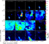 |
Fig. D.1 Channel map of the 12CO(1 − 0) observationscarried out with the IRAM 30 m telescope. The 10′ × 10′ field is shown in its entirety. Each panel represent the emission integrated over an interval of 0.5 km s−1 around a given velocity along the line of sight. Velocities are indicated on the top left corner of each panel. Velocity channels represented on this figure are between v = − 20 km s−1 and v = 8 km s−1, covering all the spectral features detected toward IC443G. |
 |
Fig. D.2 Channel map of the 13CO(1−0) observationscarried out with the IRAM 30 m telescope. The 10′ × 10′ field is entirely displayed. Each panel represent the emission integrated over an interval of velocity along the line of sight. Velocities are indicated on the top left corner of each panel. Velocity channels represented in this figure are between v = − 24 km s−1 and v = +12 km s−1, covering all the spectral features detected toward the extended G region. |
 |
Fig. D.3 Channel map of the 12CO(2−1) observationscarried out with the APEX. The 10′ × 10′ field is shown in its entirety. Each panel represent the emission integrated over an interval of velocity along the line of sight. Velocities are indicated on the top left corner of each panel. Velocity channels represented in this figure are between v = − 24 km s−1 and v = +12 km s−1, covering all the spectral features detected toward the extended G region. |
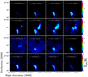 |
Fig. D.4 Channel map of the 12CO(3−2) observationscarried out with APEX. The 10′ × 10′ field is shown in its entirety. Each panel represent the emission integrated over an interval of velocity along the line of sight. Velocities are indicated on the top left corner of each panel. Velocity channels represented in this figure are between v = − 24 km s−1 and v = +12 km s−1, covering all the spectral features detected toward the extended G region. |
Appendix E Spectralenergy distributions of protostar candidates
 |
Fig. E.1 Spectral energy distributions of 17 protostar candidates. Their corresponding ID in Tables G.2and G.1 are indicated in the top left corner of each box when available (marked with an “*” if not corresponding to any point sources identified by a label). Red markers correspond to 2MASS photometric measures and black markers correspond to WISE measures. |
Appendix F Observational measure of the optical depth
 |
Fig. F.1 Spectra obtained over the region of the four boxes defined in Fig. 6, for the following lines: 12CO (in black), 13CO (in blue), and C18O (in red). First row: (1–0) transition, second row: (2–1) transition, and third row: (3–2) transition for: A, the cloudlet; B, the ring-likestructure; C, the shocked clump; and D, the shocked knot. Spectral cubes were resampled to allow a direct comparison between the different spectra. Spatial resolutions of all transitions were modified to the nominal resolution of C18O (2–1), θ = 30.2′′. Spectral resolution were set to 0.5 km s−1 for the IRAM 30 m data, and 0.25 km s−1 for APEX data. On both panels, the vLSR of IC443 is indicated with a vertical dashed line (at − 4.5 km s−1). The black data points with error bars represent the measurements of the optical depth τ corresponding to each channel of these spectra resampled with a spectral resolution of 2 km s−1, using the [12CO]/[13CO] ratio as a tracer, and the red data points represent the measurements of the optical depth obtained using the [12CO]/[C18O] ratio. The adopted values for the isotopic ratios are based on the results of Sect. 4.2.1 and indicated in Table 5. |
Appendix G WISE and 2MASS based classification of infrared point sources in the extended G region
Infrared photometric magnitudes of YSO candidates detected by WISE in the extended G region.
Infrared photometric magnitudes of YSO candidates detected by 2MASS in the extended G region.
References
- Abdo, A. A., Ackermann, M., Ajello, M., et al. 2010, ApJ, 712, 459 [NASA ADS] [CrossRef] [Google Scholar]
- Ackermann, M., Ajello, M., Allafort, A., et al. 2013, Science, 339, 807 [NASA ADS] [CrossRef] [PubMed] [Google Scholar]
- Adams, F. C., Lada, C. J., & Shu, F. H. 1987, ApJ, 312, 788 [NASA ADS] [CrossRef] [Google Scholar]
- Alarie, A., & Drissen, L. 2019, MNRAS, 489, 3042 [CrossRef] [Google Scholar]
- Albert, J., Aliu, E., Anderhub, H., et al. 2007, ApJ, 664, L87 [NASA ADS] [CrossRef] [Google Scholar]
- Ambrocio-Cruz, P., Rosado, M., de la Fuente, E., Silva, R., & Blanco-Piñon, A. 2017, MNRAS, 472, 51 [NASA ADS] [CrossRef] [Google Scholar]
- Astropy Collaboration (Robitaille, T. P., et al.) 2013, A&A, 558, A33 [NASA ADS] [CrossRef] [EDP Sciences] [Google Scholar]
- Astropy Collaboration (Price-Whelan, A. M., et al.) 2018, AJ, 156, 123 [Google Scholar]
- Bailer-Jones, C. A. L., Rybizki, J., Fouesneau, M., Mantelet, G., & Andrae, R. 2018, AJ, 156, 58 [NASA ADS] [CrossRef] [Google Scholar]
- Bocchino, F., & Bykov, A. M. 2000, A&A, 362, L29 [NASA ADS] [Google Scholar]
- Bocchino, F., & Bykov, A. M. 2003, A&A, 400, 203 [NASA ADS] [CrossRef] [EDP Sciences] [Google Scholar]
- Bolatto, A. D., Wolfire, M., & Leroy, A. K. 2013, ARA&A, 51, 207 [Google Scholar]
- Braun, R., & Strom, R. G. 1986, A&A, 164, 193 [NASA ADS] [Google Scholar]
- Bron, E., Daudon, C., Pety, J., et al. 2018, A&A, 610, A12 [NASA ADS] [CrossRef] [EDP Sciences] [Google Scholar]
- Burton, M. G., Hollenbach, D. J., Haas, M. R., & Erickson, E. F. 1990, ApJ, 355, 197 [NASA ADS] [CrossRef] [Google Scholar]
- Bykov, A. M., Ellison, D. C., Marcowith, A., & Osipov, S. M. 2018, Space Sci. Rev., 214, 41 [NASA ADS] [CrossRef] [Google Scholar]
- Cardillo, M., Amato, E., & Blasi, P. 2016, A&A, 595, A58 [NASA ADS] [CrossRef] [EDP Sciences] [Google Scholar]
- Carter, M., Lazareff, B., Maier, D., et al. 2012, A&A, 538, A89 [NASA ADS] [CrossRef] [EDP Sciences] [Google Scholar]
- Castelletti, G., Dubner, G., Clarke, T., & Kassim, N. E. 2011, A&A, 534, A21 [NASA ADS] [CrossRef] [EDP Sciences] [Google Scholar]
- Celli, S., Morlino, G., Gabici, S., & Aharonian, F. A. 2019, MNRAS, 487, 3199 [CrossRef] [Google Scholar]
- Cesarsky, D., Cox, P., Pineau des Forêts, G., et al. 1999, A&A, 348, 945 [NASA ADS] [Google Scholar]
- Cherchneff, I. 2014, ArXiv e-prints, [arXiv:1405.1216] [Google Scholar]
- Chevalier, R. A. 1974, ApJ, 188, 501 [NASA ADS] [CrossRef] [Google Scholar]
- Claussen, M. J., Frail, D. A., Goss, W. M., & Gaume, R. A. 1997, ApJ, 489, 143 [NASA ADS] [CrossRef] [Google Scholar]
- Dame, T. M., Hartmann, D., & Thaddeus, P. 2001, ApJ, 547, 792 [NASA ADS] [CrossRef] [Google Scholar]
- Denoyer, L. K. 1978, MNRAS, 183, 187 [NASA ADS] [CrossRef] [Google Scholar]
- Denoyer, L. K. 1979a, ApJ, 232, L165 [NASA ADS] [CrossRef] [Google Scholar]
- Dickman, R. L., Snell, R. L., Ziurys, L. M., & Huang, Y.-L. 1992, ApJ, 400, 203 [NASA ADS] [CrossRef] [Google Scholar]
- Draine, B. T. 2011, Physics of the Interstellar and Intergalactic Medium (Princeton: Princeton University Press) [Google Scholar]
- Dunham, M. M., Allen, L. E., Evans, Neal J., I., et al. 2015, ApJS, 220, 11 [NASA ADS] [CrossRef] [Google Scholar]
- Egron, E., Pellizzoni, A., Iacolina, M. N., et al. 2017, MNRAS, 470, 1329 [NASA ADS] [CrossRef] [Google Scholar]
- Endres, C. P., Schlemmer, S., Schilke, P., Stutzki, J., & Müller, H. S. P. 2016, J. Mol. Spectr., 327, 95 [NASA ADS] [CrossRef] [Google Scholar]
- Esposito, J. A., Hunter, S. D., Kanbach, G., & Sreekumar, P. 1996, ApJ, 461, 820 [NASA ADS] [CrossRef] [Google Scholar]
- Evans, Neal J., I., Dunham, M. M., Jørgensen, J. K., et al. 2009, ApJS, 181, 321 [NASA ADS] [CrossRef] [Google Scholar]
- Fesen, R. A., & Kirshner, R. P. 1980, ApJ, 242, 1023 [NASA ADS] [CrossRef] [Google Scholar]
- Fischer, W. J., Padgett, D. L., Stapelfeldt, K. L., & Sewiło, M. 2016, ApJ, 827, 96 [NASA ADS] [CrossRef] [Google Scholar]
- Frail, D. A., Goss, W. M., Reynoso, E. M., et al. 1996, AJ, 111, 1651 [NASA ADS] [CrossRef] [Google Scholar]
- François, P., Matteucci, F., Cayrel, R., et al. 2004, A&A, 421, 613 [NASA ADS] [CrossRef] [EDP Sciences] [Google Scholar]
- Frerking, M. A., Langer, W. D., & Wilson, R. W. 1982, ApJ, 262, 590 [NASA ADS] [CrossRef] [Google Scholar]
- Gabici, S., Aharonian, F. A., & Casanova, S. 2009, MNRAS, 396, 1629 [NASA ADS] [CrossRef] [Google Scholar]
- Gabici, S., Evoli, C., Gaggero, D., et al. 2019, Int. J. Mod. Phys. D., 28, 1930022–339 [CrossRef] [Google Scholar]
- Glassgold, A. E., Huggins, P. J., & Langer, W. D. 1985, ApJ, 290, 615 [NASA ADS] [CrossRef] [Google Scholar]
- Goldsmith, P. F., & Langer, W. D. 1999, ApJ, 517, 209 [NASA ADS] [CrossRef] [Google Scholar]
- Gordon, M. A., & Burton, W. B. 1976, ApJ, 208, 346 [NASA ADS] [CrossRef] [Google Scholar]
- Goss, W. M. 1968, ApJS, 15, 131 [NASA ADS] [CrossRef] [Google Scholar]
- Greene, T. P., Wilking, B. A., Andre, P., Young, E. T., & Lada, C. J. 1994, ApJ, 434, 614 [NASA ADS] [CrossRef] [Google Scholar]
- Grenier, I. A., Black, J. H., & Strong, A. W. 2015, ARA&A, 53, 199 [NASA ADS] [CrossRef] [Google Scholar]
- Gutermuth, R. A., Megeath, S. T., Myers, P. C., et al. 2009, ApJS, 184, 18 [NASA ADS] [CrossRef] [Google Scholar]
- Hanabata, Y., Katagiri, H., Hewitt, J. W., et al. 2014, ApJ, 786, 145 [NASA ADS] [CrossRef] [Google Scholar]
- Harris, D. E. 1962, ApJ, 135, 661 [NASA ADS] [CrossRef] [Google Scholar]
- Herbst, W., & Assousa, G. E. 1977, ApJ, 217, 473 [NASA ADS] [CrossRef] [Google Scholar]
- Hester, J. J. 1987, ApJ, 314, 187 [NASA ADS] [CrossRef] [Google Scholar]
- Hewitt, J. W., Yusef-Zadeh, F., Wardle, M., Roberts, D. A., & Kassim, N. E. 2006, ApJ, 652, 1288 [NASA ADS] [CrossRef] [Google Scholar]
- Hewitt, J. W., Yusef-Zadeh, F., & Wardle, M. 2008, ApJ, 683, 189 [NASA ADS] [CrossRef] [Google Scholar]
- Hewitt, J. W., Yusef-Zadeh, F., & Wardle, M. 2009, ApJ, 706, L270 [NASA ADS] [CrossRef] [Google Scholar]
- Heyminck, S., Kasemann, C., Güsten, R., de Lange, G., & Graf, U. U. 2006, A&A, 454, L21 [NASA ADS] [CrossRef] [EDP Sciences] [Google Scholar]
- Hezareh, T., Wiesemeyer, H., Houde, M., Gusdorf, A., & Siringo, G. 2013, A&A, 558, A45 [NASA ADS] [CrossRef] [EDP Sciences] [Google Scholar]
- Hildebrand, R. H. 1983, QJRAS, 24, 267 [NASA ADS] [Google Scholar]
- Hoffman, I. M., Goss, W. M., Brogan, C. L., Claussen, M. J., & Richards, A. M. S. 2003, ApJ, 583, 272 [NASA ADS] [CrossRef] [Google Scholar]
- Hollenbach, D., & McKee, C. F. 1989, ApJ, 342, 306 [NASA ADS] [CrossRef] [Google Scholar]
- Huang, Y. L., Dickman, R. L., & Snell, R. L. 1986, ApJ, 302, L63 [NASA ADS] [CrossRef] [Google Scholar]
- Hunter, J. D. 2007, Comput. Sci. Eng., 9, 90 [NASA ADS] [CrossRef] [Google Scholar]
- Indriolo, N., Blake, G. A., Goto, M., et al. 2010, ApJ, 724, 1357 [NASA ADS] [CrossRef] [Google Scholar]
- Jones, E., Oliphant, T., Peterson, P., et al. 2001, SciPy: Open Source Scientific Tools for Python [Google Scholar]
- Klein, B., Hochgürtel, S., Krämer, I., et al. 2012, A&A, 542, L3 [NASA ADS] [CrossRef] [EDP Sciences] [Google Scholar]
- Koenig, X. P., & Leisawitz, D. T. 2014, ApJ, 791, 131 [NASA ADS] [CrossRef] [Google Scholar]
- Koenig, X. P., Leisawitz, D. T., Benford, D. J., et al. 2012, ApJ, 744, 130 [NASA ADS] [CrossRef] [Google Scholar]
- Koo, B.-C., McKee, C. F., Lee, J.-J., et al. 2008, ApJ, 673, L147 [NASA ADS] [CrossRef] [Google Scholar]
- Koo, B.-C., Heiles, C., Stanimirović, S., & Troland, T. 2010, AJ, 140, 262 [NASA ADS] [CrossRef] [Google Scholar]
- Lada, C. J., & Adams, F. C. 1992, ApJ, 393, 278 [NASA ADS] [CrossRef] [Google Scholar]
- Langer, W. D., & Penzias, A. A. 1993, ApJ, 408, 539 [NASA ADS] [CrossRef] [Google Scholar]
- Larson, R. B. 1981, MNRAS, 194, 809 [CrossRef] [Google Scholar]
- Lee, J.-J., Koo, B.-C., Yun, M. S., et al. 2008, AJ, 135, 796 [NASA ADS] [CrossRef] [Google Scholar]
- Lee, J.-J., Koo, B.-C., Snell, R. L., et al. 2012, ApJ, 749, 34 [NASA ADS] [CrossRef] [Google Scholar]
- Lefloch, B., & Lazareff, B. 1994, A&A, 289, 559 [NASA ADS] [Google Scholar]
- Lockett, P., Gauthier, E., & Elitzur, M. 1999, ApJ, 511, 235 [NASA ADS] [CrossRef] [Google Scholar]
- Loru, S., Pellizzoni, A., Egron, E., et al. 2019, MNRAS, 482, 3857 [CrossRef] [Google Scholar]
- Mac Low, M.-M., & Klessen, R. S. 2004, Rev. Mod. Phys., 76, 125 [NASA ADS] [CrossRef] [Google Scholar]
- Madau, P., & Dickinson, M. 2014, ARA&A, 52, 415 [NASA ADS] [CrossRef] [Google Scholar]
- Micelotta, E. R., Matsuura, M., & Sarangi, A. 2018, Space Sci. Rev., 214, 53 [CrossRef] [Google Scholar]
- Mihalas, D. 1978, Stellar Atmospheres (San Francisco, USA: W.H. Freeman) [Google Scholar]
- Minkowski, R. 1946, PASP, 58, 305 [NASA ADS] [CrossRef] [Google Scholar]
- Montmerle, T. 1979, ApJ, 231, 95 [NASA ADS] [CrossRef] [Google Scholar]
- Moorhouse, A., Brand, P. W. J. L., Geballe, T. R., & Burton, M. G. 1991, MNRAS, 253, 662 [NASA ADS] [CrossRef] [Google Scholar]
- Motte, F., Nony, T., Louvet, F., et al. 2018, Nat. Astron., 2, 478 [NASA ADS] [CrossRef] [Google Scholar]
- Muders, D., Hafok, H., Wyrowski, F., et al. 2006, A&A, 454, L25 [NASA ADS] [CrossRef] [EDP Sciences] [Google Scholar]
- Mufson, S. L., McCollough, M. L., Dickel, J. R., et al. 1986, AJ, 92, 1349 [NASA ADS] [CrossRef] [Google Scholar]
- Müller, H. S. P., Thorwirth, S., Roth, D. A., & Winnewisser, G. 2001, A&A, 370, L49 [NASA ADS] [CrossRef] [EDP Sciences] [Google Scholar]
- Müller, H. S. P., Schlöder, F., Stutzki, J., & Winnewisser, G. 2005, J. Mol. Struct., 742, 215 [NASA ADS] [CrossRef] [Google Scholar]
- Neufeld, D., Bergin, E., Hollenbach, D., et al. 2004, IRS Spectroscopy of Shocked Molecular Gas in Supernova Remnants: Probing the Interaction of a Supernova with a Molecular Cloud, Spitzer Proposal [Google Scholar]
- Neufeld, D. A., Hollenbach, D. J., Kaufman, M. J., et al. 2007, ApJ, 664, 890 [NASA ADS] [CrossRef] [MathSciNet] [Google Scholar]
- Noriega-Crespo, A., Hines, D. C., Gordon, K., et al. 2009, in The Evolving ISM in the Milky Way and Nearby Galaxies, 46 [Google Scholar]
- Olbert, C. M., Clearfield, C. R., Williams, N. E., Keohane, J. W., & Frail, D. A. 2001a, ApJ, 554, L205 [NASA ADS] [CrossRef] [Google Scholar]
- Olbert, C. M., Clearfield, C. R., Williams, N. E., Keohane, J. W., & Frail, D. A. 2001b, AIP Conf. Ser., 565, 341 [CrossRef] [Google Scholar]
- Padovani, M., Hennebelle, P., Marcowith, A., & Ferrière, K. 2015, A&A, 582, L13 [NASA ADS] [CrossRef] [EDP Sciences] [Google Scholar]
- Padovani, M., Marcowith, A., Hennebelle, P., & Ferrière, K. 2016, A&A, 590, A8 [NASA ADS] [CrossRef] [EDP Sciences] [Google Scholar]
- Padovani, M., Marcowith, A., Sánchez-Monge, Á., Meng, F., & Schilke, P. 2019, A&A, 630, A72 [NASA ADS] [CrossRef] [EDP Sciences] [Google Scholar]
- Parker, R. A. R. 1963, PhD thesis, California Institute of Technology, USA [Google Scholar]
- Parker, R. A. R. 1964, ApJ, 139, 493 [CrossRef] [Google Scholar]
- Petre, R., Szymkowiak, A. E., Seward, F. D., & Willingale, R. 1988, ApJ, 335, 215 [NASA ADS] [CrossRef] [Google Scholar]
- Pickett, H. M., Poynter, R. L., Cohen, E. A., et al. 1998, J. Quant. Spectr. Rad. Transf., 60, 883 [Google Scholar]
- Pinheiro Gonçalves, D., Noriega-Crespo, A., Paladini, R., Martin, P. G., & Carey, S. J. 2011, AJ, 142, 47 [NASA ADS] [CrossRef] [Google Scholar]
- Reach, W. T., Tram, L. N., Richter, M., Gusdorf, A., & DeWitt, C. 2019, ApJ, 884, 81 [CrossRef] [Google Scholar]
- Rho, J., & Petre, R. 1998, ApJ, 503, L167 [NASA ADS] [CrossRef] [Google Scholar]
- Rho, J., Jarrett, T. H., Cutri, R. M., & Reach, W. T. 2001, ApJ, 547, 885 [NASA ADS] [CrossRef] [Google Scholar]
- Roueff, A., Gerin, M., Gratier, P., et al. 2020, A&A, in press, https://doi.org/ 10.1051/0004-6361/202037776 [Google Scholar]
- Sarangi, A., Matsuura, M., & Micelotta, E. R. 2018, Space Sci. Rev., 214, 63 [CrossRef] [Google Scholar]
- Seta, M., Hasegawa, T., Dame, T. M., et al. 1998, ApJ, 505, 286 [NASA ADS] [CrossRef] [Google Scholar]
- Shinn, J.-H., Koo, B.-C., Seon, K.-I., & Lee, H.-G. 2011, ApJ, 732, 124 [CrossRef] [Google Scholar]
- Snell, R. L., Hollenbach, D., Howe, J. E., et al. 2005, ApJ, 620, 758 [NASA ADS] [CrossRef] [Google Scholar]
- Sobolev, V. V. 1960, Moving Envelopes of Stars (Harvard University Press) [Google Scholar]
- Su, Y., Fang, M., Yang, J., Zhou, P., & Chen, Y. 2014, ApJ, 788, 122 [NASA ADS] [CrossRef] [Google Scholar]
- Surdej, J. 1977, A&A, 60, 303 [NASA ADS] [Google Scholar]
- Tang, X. 2019, MNRAS, 482, 3843 [CrossRef] [Google Scholar]
- Tatischeff, V., & Gabici, S. 2018, Ann. Rev. Nucl. Part. Sci., 68, 377 [CrossRef] [Google Scholar]
- Tauber, J. A., Snell, R. L., Dickman, R. L., & Ziurys, L. M. 1994, ApJ, 421, 570 [CrossRef] [Google Scholar]
- Tavani, M., Giuliani, A., Chen, A. W., et al. 2010, ApJ, 710, L151 [NASA ADS] [CrossRef] [Google Scholar]
- Torres, D. F., Marrero, A. Y. R., & de Cea Del Pozo, E. 2010, MNRAS, 408, 1257 [NASA ADS] [CrossRef] [Google Scholar]
- Troja, E., Bocchino, F., & Reale, F. 2006, ApJ, 649, 258 [NASA ADS] [CrossRef] [Google Scholar]
- Troja, E., Bocchino, F., Miceli, M., & Reale, F. 2008, A&A, 485, 777 [NASA ADS] [CrossRef] [EDP Sciences] [Google Scholar]
- van der Tak, F. F. S., Black, J. H., Schöier, F. L., Jansen, D. J., & van Dishoeck, E. F. 2007, A&A, 468, 627 [NASA ADS] [CrossRef] [EDP Sciences] [Google Scholar]
- van der Walt, S., Colbert, S. C., & Varoquaux, G. 2011, Comput. Sci. Eng., 13, 22 [Google Scholar]
- van Dishoeck, E. F., Jansen, D. J., & Phillips, T. G. 1993, A&A, 279, 541 [NASA ADS] [Google Scholar]
- VERITAS Collaboration (Humensky, B.) 2015, 34th International Cosmic Ray Conference (ICRC2015), 875 [Google Scholar]
- Wang, Z., & Scoville, N. Z. 1992, ApJ, 386, 158 [NASA ADS] [CrossRef] [Google Scholar]
- Wang, Z. R., Asaoka, I., Hayakawa, S., & Koyama, K. 1992, PASJ, 44, 303 [NASA ADS] [Google Scholar]
- Wardle, M. 1999, ApJ, 525, L101 [NASA ADS] [CrossRef] [PubMed] [Google Scholar]
- Wardle, M., & Yusef-Zadeh, F. 2002, Science, 296, 2350 [NASA ADS] [CrossRef] [Google Scholar]
- Welsh, B. Y., & Sallmen, S. 2003, A&A, 408, 545 [NASA ADS] [CrossRef] [EDP Sciences] [Google Scholar]
- Wenger, T. V., Balser, D. S., Anderson, L. D., & Bania, T. M. 2018, ApJ, 856, 52 [NASA ADS] [CrossRef] [Google Scholar]
- White, G. J., Rainey, R., Hayashi, S. S., & Kaifu, N. 1987, A&A, 173, 337 [NASA ADS] [Google Scholar]
- Wilking, B. A., Lada, C. J., & Young, E. T. 1989, ApJ, 340, 823 [NASA ADS] [CrossRef] [Google Scholar]
- Wilson, T. L., & Rood, R. 1994, ARA&A, 32, 191 [NASA ADS] [CrossRef] [Google Scholar]
- Wood, C. A., Mufson, S. L., & Dickel, J. R. 1991, AJ, 102, 224 [NASA ADS] [CrossRef] [Google Scholar]
- Wright, E. L., Eisenhardt, P. R. M., Mainzer, A. K., et al. 2010, AJ, 140, 1868 [Google Scholar]
- Xu, J.-L., Wang, J.-J., & Miller, M. 2011, ApJ, 727, 81 [NASA ADS] [CrossRef] [Google Scholar]
- York, D. G., Adelman, J., Anderson, John E., J., et al. 2000, AJ, 120, 1579 [CrossRef] [Google Scholar]
- Yusef-Zadeh, F., Wardle, M., Rho, J., & Sakano, M. 2003, ApJ, 585, 319 [NASA ADS] [CrossRef] [Google Scholar]
- Zhang, Z., Gao, Y., & Wang, J. 2010, Sci. China Phys. Mech. Astron., 53, 1357 [Google Scholar]
- Ziurys, L. M., Snell, R. L., & Dickman, R. L. 1988, Recent Molecular Studies of Supernova Remnant IC443 – Some New Results for Shock Chemistry, eds. R. L. Dickman, R. L. Snell, & J. S. Young, 315, 184 [Google Scholar]
This publication is partly based on data acquired under project M9508A_102 with the Atacama Pathfinder EXperiment (APEX). APEX is a collaboration between the Max-Planck-Institut für Radioastronomie (MPIfR), the European Southern Observatory, and the Onsala Space Observatory.
APEX telescope efficiencies are taken from http://www.apex-telescope.org/telescope/efficiency/index.php, and IRAM telescope efficiencies are taken from https://www.iram-institute.org/medias/uploads/eb2013-v8.2.pdf
The Grenoble Image and Line Data Analysis Software is developed and maintained by IRAM to reduce and analyze data obtained with the 30 m telescope and Plateau de Bure interferometer. See www.iram.fr/IRAMFR/GILDAS
This work is based on observations out under project number 169-18 with the IRAM 30 m telescope. IRAM is supported by INSU/CNRS (France), MPG (Germany) and IGN (Spain).
Python Core Team (2015). Python: a dynamic, open source programming language. Python Software Foundation. https://www.python.org/
The Python module scipy.optimize.curve_fit uses the Levenberg-Marquardt least-squares curve fitting algorithm.
We computed the partition function taking into account the first 40 upper rotational levels of 12CO taken from the Cologne Database for Molecular Spectroscopy and Jet Propulsion Laboratory database. The thermal energy of the 40th level is E40 = 4513 K.
The Einstein coefficients Aij are given in Table 1, and the collisional excitation rates Cij are taken from the Cologne Database for Molecular Spectroscopy and Jet Propulsion Laboratory database.
All Tables
Observed lines and corresponding telescope parameters for the observations of the extended G region of IC443.
Infrared photometric magnitudes of YSO candidates detected by WISE in the extended G region.
Infrared photometric magnitudes of YSO candidates detected by 2MASS in the extended G region.
All Figures
|
Fig. 1 Spitzer/MIPS map (colors) of IC443 at 24 μm (Pinheiro Gonçalves et al. 2011; Noriega-Crespo et al. 2009). In contours, the VLA emission map shows the morphologyof the synchrotron emission at 330 MHz (Claussen et al. 1997). The white dot indicates the position of the PWN wind (Olbert et al. 2001b). The red box represents one of the fields observed by Spitzer-IRS (Neufeld et al. 2004), corresponding roughly to the G region defined by Huang et al. (1986). The white box represents the 10′ × 10′ field of our observations called “the extended G region”. The IRAM 30 m instrumental beam diameter corresponding to the 12CO(1–0) transition and the size of the typical PSF of γ-ray telescopes (5′) are indicated by white disks in the bottom left corner of the figure. |
| In the text | |
|
Fig. 2 Channel maps of the 12CO(2–1) observations carried out with the IRAM 30 m telescope. Each panel represents the emission integratedover an interval of velocity along the line of sight. Velocity intervals are indicated on the top left corner of each panel. Velocity channels represented in this figure are between v = − 24 km s−1 and v = +12 km s−1, covering all the spectral features detected toward the extended G region. Structures described in Sect. 3.2are indicated with the corresponding letters. |
| In the text | |
|
Fig. 3 Two-dimensional histogram of |
| In the text | |
|
Fig. 4 Left: 0th moment of the 12CO(2–1) observationscarried out with the IRAM 30 m over the extended G region. This map corresponds to the signal integrated in the velocity interval [−40; +30] km s−1. The color scale used to represent data is logarithmic to enhance the dynamic range and emphasize the fainter molecular cloudlet. Right: composite image of our field of observations in the extended G region, using an IRAM 30 m data cube as well as Spitzer-MIPS data; 12CO(2–1) ([−40, +30] km s−1 as in the left panel) is coded in red, MIPS-24 μm in blue, and 13CO(1–0) [−4.0, −2.5] km s−1, corresponding to the emission spatially and kinematically associated with the ambient cloud described by Lee et al. (2012) in green. Color scale levels are based on the minimum and maximum value of each map. |
| In the text | |
|
Fig. 5 Left: first moment map of the IRAM 30 m 12CO(2–1) data cube. Center: second moment map of the same data cube. Right, top panel: zoom into the dashed box on the first moment map of the APEX 12CO (3–2) data cube to enhance the spectral resolution. Right top and bottom panels: first and second moment maps of the APEX 12CO(3–2) data cube into the dashed box shown in the right and middle panels, respectively. The color bar of the left figure is centered on the velocity of IC443 in the local standard of rest, vLSR = −4.5 km s−1. |
| In the text | |
|
Fig. 6 Spitzer/MIPS map at 24.0 μm. In black contours, the emission of 12CO(2–1) observedwith the IRAM 30 m is shown over different intervals of velocities: A [−7; −5] km s−1 (cloudlet); B[−5.5; −4.5] km s−1 (ring-like structure); and C and D [−40; +30] km s−1 (shocked clump and shocked knot). The white boxes represent the area where the signal corresponding to each structure is integrated. The beam diameter of the IRAM 30 m observations of 12CO(2–1) is shown in the bottom left corner. |
| In the text | |
|
Fig. 7 Spectra averaged over the regions of the cloudlet (left panels) and the ring (right panels) defined in Fig. 6 for the following lines: 12CO (1–0), 13CO (1–0) and C18O(1–0) (in black, IRAM-30m); 12CO(2–1), 13CO (2–1) and C18O(2–1) (in blue, APEX); 12CO(3–2) and 13CO(3–2) (in grey, APEX). Spectral cubes were resampled to allow a direct comparison between the different spectra. Spatial resolutions of all transitions were modified to the nominal resolution of C18O (2–1), θ = 30.2′′. Spectral resolutions were set to 0.5 km s−1 for IRAM 30m data and 0.25 km s−1 for APEX data. On both panels, the vLSR of IC443 is indicated with a vertical dashed line (at − 4.5 km s−1). |
| In the text | |
|
Fig. 8 Spectra averaged over the region of the shocked clump (left) and shocked knot (right) defined in Fig. 6 for the following lines: 12CO (1–0), 13CO (1–0) and C18O(1–0) (in black, IRAM 30 m); 12CO(2–1), 13CO (2–1) and C18O(2–1) (in blue, APEX); 12CO(3–2) and 13CO(3–2) (in grey, APEX). Spectral cubes were resampled to allow a direct comparison between the different spectra. Spatial resolutions of all transitions were modified to the nominal resolution of C18O (2–1), θ = 30.2′′. Spectral resolutions were set to 0.5 km s−1 for IRAM 30m data and 0.25 km s−1 for APEX data. On both panels, the vLSR of IC443 is indicated with a vertical dashed line (at − 4.5 km s−1). |
| In the text | |
|
Fig. 9 Data histograms and LTE models of the emission of the rotational transitions of 12CO and its isotopologs mapped in the extended G field with the IRAM 30 m and APEX: 1. 13CO (1–0) vs. 12CO(1–0); 2. 13CO (1–0) vs. C18O(1–0); 3. [13CO(1–0)] / [C18O (1–0)] vs. [12CO(1–0)] / [13CO (1–0)]; and 4. 12CO(3–2) / 12CO (2–1) vs. 12CO(2–1) / 12CO (1–0). The color map corresponds to the amount of data points (line of sight and velocity channels) that fall into a given bin of the histogram. The curves represent families of models of the LTE intensity as a function of the kinetic temperature of 13CO. The arrows indicate the direction in which the kinetic temperature grows along a given curve. Control parameters of the LTEmodels are given in Table 4 for each histogram. The dashed black lines represent the 3σ detection level for each axis (histograms 1 and 2). |
| In the text | |
|
Fig. 10 Average population diagrams of 12CO corrected for optical depth. The measured average, first quartile, third quartile, fifth percentile, and 95th percentile associated with our sample of level populations corresponding to Jup = 1, Jup = 2, and Jup = 3 are indicated for two adopted values of the 12CO/13CO isotopic ratio (12CO/13CO = 60 in black, 12CO/13CO = 100 in red). The black solid line represents the linear fit of the black data points. The boundaries of the filled areas are defined by the linear fits corresponding to the first and third quartiles for each value of the isotopic ratio adopted. The 5th percentile and 95th percentile are indicated by the caps, the first quartile and third quartile are indicated by the ends of the box, and the average is indicated by the cap inside of the box. Each diagram accounts for a sample of measurements performed in one of the spatial boxes defined in Fig. 6 and integration ranges defined in Table 6: (a) the shocked clump, (b) the cloudlet, (c) the ring, (d) the ambient cloud, and (e) the shocked knot. |
| In the text | |
|
Fig. 11 Average population diagrams of 13CO. The measured average, first quartile, third quartile, 5th percentile, and 95th percentile associated with our sample of measured level populations are indicated for each level. The black solid line represents the linear fit of the average data points. The boundaries of the filled areas are defined by the linear fits corresponding to the first and third quartiles. Each diagram accounts for a sample of measurements performed in one of the spatial boxes, as in Fig. 10. |
| In the text | |
|
Fig. 12 Diagrams of χ2 minimization of the comparison between 1 × 200 × 200 LVG grids modeled with sets of parameters ( |
| In the text | |
|
Fig. 13 Left: WISE census of protostar candidates in the extended G region. Cyan dots indicate Class II candidates, red dots indicate Class I candidates, and grey dots indicate point sources detected by WISE and rejected by our color–color filtering based on photometric bands W1, W2, and W3. Right: 2MASS census of protostar candidates in the extended G region. Cyan dots represent CTTS candidates, red dots denote HaeBe candidates, magenta dots indicate YSO candidates, and grey dots indicate point sources detected by 2MASS and rejected by our JHK color–color filtering. |
| In the text | |
|
Fig. 14 Top left panel: WISE census of Class I and Class II protostar candidates, with shock emission indicated. Based on the selection criteria by Fischer et al. (2016). Top right panel: 2MASS census of YSO, CTTS, and HAeBe candidates. Based on the selection criteria by Xu et al. (2011). Center left panel: close-up on the box corresponding to group 2. Center rightpanel: transition disks, AGB star, star-forming galaxies emission, and PAH emission candidates, based on the selectioncriteria by Fischer et al. (2016); and Gaia point sources. Bottom panel: close-up on the box corresponding to group 1. On all panels, triangle-shaped markers correspond to well-detected point sources, and circle-shaped markers (labels marked with a “*”) correspond to point sources that were flagged for contamination by extended emission. Filled markers represent point sources that were detected both by 2MASS and WISE. |
| In the text | |
|
Fig. C.1 Spatial distribution of protostar candidates in our 10′ × 10′ field of observations. Left: Class I and Class II candidates detected by WISE. Right: YSO candidates detected by 2MASS. White contours represent the CO(2–1) emission in the velocity range [−7, +3] km s−1. |
| In the text | |
|
Fig. D.1 Channel map of the 12CO(1 − 0) observationscarried out with the IRAM 30 m telescope. The 10′ × 10′ field is shown in its entirety. Each panel represent the emission integrated over an interval of 0.5 km s−1 around a given velocity along the line of sight. Velocities are indicated on the top left corner of each panel. Velocity channels represented on this figure are between v = − 20 km s−1 and v = 8 km s−1, covering all the spectral features detected toward IC443G. |
| In the text | |
|
Fig. D.2 Channel map of the 13CO(1−0) observationscarried out with the IRAM 30 m telescope. The 10′ × 10′ field is entirely displayed. Each panel represent the emission integrated over an interval of velocity along the line of sight. Velocities are indicated on the top left corner of each panel. Velocity channels represented in this figure are between v = − 24 km s−1 and v = +12 km s−1, covering all the spectral features detected toward the extended G region. |
| In the text | |
|
Fig. D.3 Channel map of the 12CO(2−1) observationscarried out with the APEX. The 10′ × 10′ field is shown in its entirety. Each panel represent the emission integrated over an interval of velocity along the line of sight. Velocities are indicated on the top left corner of each panel. Velocity channels represented in this figure are between v = − 24 km s−1 and v = +12 km s−1, covering all the spectral features detected toward the extended G region. |
| In the text | |
|
Fig. D.4 Channel map of the 12CO(3−2) observationscarried out with APEX. The 10′ × 10′ field is shown in its entirety. Each panel represent the emission integrated over an interval of velocity along the line of sight. Velocities are indicated on the top left corner of each panel. Velocity channels represented in this figure are between v = − 24 km s−1 and v = +12 km s−1, covering all the spectral features detected toward the extended G region. |
| In the text | |
|
Fig. E.1 Spectral energy distributions of 17 protostar candidates. Their corresponding ID in Tables G.2and G.1 are indicated in the top left corner of each box when available (marked with an “*” if not corresponding to any point sources identified by a label). Red markers correspond to 2MASS photometric measures and black markers correspond to WISE measures. |
| In the text | |
|
Fig. F.1 Spectra obtained over the region of the four boxes defined in Fig. 6, for the following lines: 12CO (in black), 13CO (in blue), and C18O (in red). First row: (1–0) transition, second row: (2–1) transition, and third row: (3–2) transition for: A, the cloudlet; B, the ring-likestructure; C, the shocked clump; and D, the shocked knot. Spectral cubes were resampled to allow a direct comparison between the different spectra. Spatial resolutions of all transitions were modified to the nominal resolution of C18O (2–1), θ = 30.2′′. Spectral resolution were set to 0.5 km s−1 for the IRAM 30 m data, and 0.25 km s−1 for APEX data. On both panels, the vLSR of IC443 is indicated with a vertical dashed line (at − 4.5 km s−1). The black data points with error bars represent the measurements of the optical depth τ corresponding to each channel of these spectra resampled with a spectral resolution of 2 km s−1, using the [12CO]/[13CO] ratio as a tracer, and the red data points represent the measurements of the optical depth obtained using the [12CO]/[C18O] ratio. The adopted values for the isotopic ratios are based on the results of Sect. 4.2.1 and indicated in Table 5. |
| In the text | |
Current usage metrics show cumulative count of Article Views (full-text article views including HTML views, PDF and ePub downloads, according to the available data) and Abstracts Views on Vision4Press platform.
Data correspond to usage on the plateform after 2015. The current usage metrics is available 48-96 hours after online publication and is updated daily on week days.
Initial download of the metrics may take a while.