| Issue |
A&A
Volume 685, May 2024
|
|
|---|---|---|
| Article Number | A131 | |
| Number of page(s) | 22 | |
| Section | Planets and planetary systems | |
| DOI | https://doi.org/10.1051/0004-6361/202347872 | |
| Published online | 17 May 2024 | |
Star-spot activity, orbital obliquity, transmission spectrum, physical properties, and transit time variations of the HATS-2 planetary system
1
Department of Physics, University of Rome “La Sapienza”,
Piazzale Aldo Moro 2,
00185
Rome,
Italy
e-mail: francesco.biagiotti@uniroma1.it
2
INAF – Istituto di Astrofisica e Planetologia Spaziali (INAF-IAPS),
Via Fosso del Cavaliere 100,
00133
Rome,
Italy
3
Department of Physics, University of Rome “Tor Vergata”,
Via della Ricerca Scientifica 1,
00133
Rome,
Italy
4
INAF – Turin Astrophysical Observatory,
via Osservatorio 20,
10025
Pino Torinese,
Italy
5
Max Planck Institute for Astronomy,
Königstuhl 17,
69117
Heidelberg,
Germany
6
Astrophysics Group, Keele University,
Keele
ST5 5BG,
UK
7
Instituto de Astronomia y Ciencias Planetarias de Atacama, Universidad de Atacama,
Copayapu 485,
Copiapo,
Chile
8
Department of Physics and Astronomy, University of Florence,
Largo Enrico Fermi 5,
50125
Firenze,
Italy
9
Centre for ExoLife Sciences, Niels Bohr Institute, University of Copenhagen,
Øster Voldgade 5,
1350
Copenhagen,
Denmark
10
Institute for Astronomy, University of Edinburgh,
Royal Observatory,
Edinburgh
EH9 3HJ,
UK
11
Department of Physics “E.R. Caianiello”, University of Salerno,
Via Giovanni Paolo II 132,
84084
Fisciano,
Italy
12
Istituto Nazionale di Fisica Nucleare, Sezione di Napoli,
Napoli,
Italy
13
Universität Hamburg, Department of Earth Sciences, Meteorological Institute,
Bundesstrasse 55,
20146
Hamburg,
Germany
14
Centre for Exoplanet Science, SUPA, School of Phys. & Astron., University of St Andrews,
North Haugh,
St Andrews
KY16 9SS,
UK
15
Millennium Institute of Astrophysics MAS,
Nuncio Monsenor Sotero Sanz 100, Of. 104, Providencia,
Santiago,
Chile
16
Instituto de Astrofísica, Pontificia Universidad Católica de Chile,
Av. Vicuña Mackenna 4860,
7820436
Macul, Santiago,
Chile
17
University of Southern Denmark, Department of Physics, Chemistry and Pharmacy,
Campusvej 55,
5230
Odense M,
Denmark
18
Astronomisches Rechen-Institut, Zentrum für Astronomie der Universität Heidelberg (ZAH),
69120
Heidelberg,
Germany
19
Astronomy Research Center, Research Institute of Basic Sciences, Seoul National University,
1 Gwanak-ro, Gwanak-gu,
Seoul
08826,
Korea
20
Centro de Astronomía, Universidad de Antofagasta,
Av. Angamos 601,
Antofagasta,
Chile
21
Departamento de Matemática y Física Aplicadas, Facultad de Ingeniería, Universidad Católica de la Santísima Concepción,
Alonso de Rivera 2850,
Concepción,
Chile
22
Department of Physics, Isfahan University of Technology,
Isfahan
84156-83111,
Iran
23
Centre for Electronic Imaging, Department of Physical Sciences, The Open University,
Milton Keynes,
MK7 6AA,
UK
24
Observatoire de Vaison-La-Romaine,
Départementale 51, près du Centre Equestre au Palis,
84110
Vaison-La-Romaine,
France
25
KNC Deep Sky Chile Observatory,
Chile
Received:
4
September
2023
Accepted:
12
January
2024
Aims. Our aim in this paper is to refine the orbital and physical parameters of the HATS-2 planetary system and study transit timing variations and atmospheric composition thanks to transit observations that span more than 10 yr and that were collected using different instruments and pass-band filters. We also investigate the orbital alignment of the system by studying the anomalies in the transit light curves induced by starspots on the photosphere of the parent star.
Methods. We analysed new transit events from both ground-based telescopes and NASA’s TESS mission. Anomalies were detected in most of the light curves and modelled as starspots occulted by the planet during transit events. We fitted the clean and symmetric light curves with the JKTEBOP code and those affected by anomalies with the PRISM+GEMC codes to simultaneously model the photometric parameters of the transits and the position, size, and contrast of each starspot.
Results. We found consistency between the values we found for the physical and orbital parameters and those from the discovery paper and ATLAS9 stellar atmospherical models. We identified different sets of consecutive starspot-crossing events that temporally occurred in less than five days. Under the hypothesis that we are dealing with the same starspots, occulted twice by the planet during two consecutive transits, we estimated the rotational period of the parent star and, in turn the projected and the true orbital obliquity of the planet. We find that the system is well aligned. We identified the possible presence of transit timing variations in the system, which can be caused by tidal orbital decay, and we derived a low-resolution transmission spectrum.
Key words: methods: data analysis / techniques: photometric / planets and satellites: gaseous planets / planets and satellites: individual: hats-2 b / stars: fundamental parameters / stars: individual: hats-2
© The Authors 2024
 Open Access article, published by EDP Sciences, under the terms of the Creative Commons Attribution License (https://creativecommons.org/licenses/by/4.0), which permits unrestricted use, distribution, and reproduction in any medium, provided the original work is properly cited.
This article is published in open access under the Subscribe to Open model. Subscribe to A&A to support open access publication.
1 Introduction
Due to their intrinsic size and proximity to their parent stars and despite their rarity, transiting hot Jupiters are a class of exoplanets that have received a great deal of attention from the scientific community since they were discovered (see e.g. Raymond & Morbidelli 2022, for a comprehensive review). Such peculiar characteristics offer many advantages from an observational point of view, and guarantee the possibility of characterising most of the physical and orbital parameters of these planets with extreme precision. They are also the best targets for atmospheric-characterisation observations, as recently demonstrated by the JWST (Ahrer et al. 2023; Rustamkulov et al. 2023; Alderson et al. 2023; Feinstein et al. 2023).
Even so, there are still some aspects of this population that are not yet well understood and are under investigation, such as those regarding the physical mechanisms that regulate the formation, accretion, and evolution processes or those that cause their migration from the snowline (~3 au) up to roughly 0.01 au from their host stars. For example, several mechanisms have been advocated that are able to shrink the orbit of a giant planet, such as dynamical interactions through planetplanet scattering (Rasio & Ford 1996; Davies et al. 2014), the Kozai mechanism (e.g. Wu & Murray 2003), and the disc-planet interaction (Lin et al. 1996; Ward 1997). However, whatever the responsible mechanism is, the planetary orbital eccentricity, e, and the spin-orbit obliquity, ψ, should be affected. If planet-planet scattering is the main mechanism that produces hot Jupiters, these scattering encounters should randomise the orbital planes, whereas disc-planet interactions force the planet’s orbit to be coplanar throughout its migration journey and we should observe an excess of flat architectures (see e.g. Biazzo et al. 2022).
In this context, we have been carrying out a more-than-10-yr project (Southworth et al. 2009) to better characterise this class of planets and with the aim of measuring their physical and orbital parameters with an accuracy of less than 5%. Our project is mainly based on high-quality photometric observations of planetary-transit events and, in several cases, was supported by high-resolution spectroscopic observations to characterise the atmospheric properties and activity host star (see e.g. Mancini et al. 2014a) or to measure the Rossitter-McLaughlin effect, which allows the measurement of the project spin-orbit alignment, λ, (see e.g. Mancini et al. 2018, 2022a).
In a few cases we faced the presence of anomalies on the transit light curves in the form of small bumps, which are attributable to the presence of single starspots or groups of starspots on the photosphere of the parent stars (see e.g. Mancini et al. 2015, 2017). These bumps appear when the planet, during its transits, temporarily hides the starspots, thus obscuring colder regions of the photosphere (Silva 2003; Winn 2010). Appropriate modelling of the light curve allows the parameters of the starspot, to be estimated, under the simplistic hypothesis that this is a single circular spot.
In the case that the orbit of the transiting planet is well aligned with the spin of its parent star and the planet has an orbital period much shorter than the stellar rotation period, then the planet can occult the same starspot multiple times. In these circumstances, the measurement of λ becomes feasible with photometric monitoring of two consecutive transits (Tregloan-Reed et al. 2013). Instead, if there is a spin-orbit misalignment, the planet will not occult the same starspot again at the subsequent transit, and we can at most obtain a lower limit on the stellar obliquity (Dai & Winn 2017).
In this work we report the results of our study of the planetary system HATS-2 that hosts a transiting hot Jupiter, HATS-2 b (Mp ≈ 1.3 MJup; Rp ≈ 1.2 RJup), which orbits around a K V dwarf star (V = 13.6 mag) in roughly 1.35 days (Mohler-Fischer et al. 2013). The authors of this discovery reported multi-band light curves of two transits in which this planet occulted starspots and, for the first time ever as far as we know, even a bright chromospheric region known as stellar plage. Using two ground-based telescopes at the ESO Observatory of La Silla, we obtained new high-quality light curves of the HATS-2 b transits and, thanks to TESS photometric data, we recognised new starspots and characterised their properties. We also reviewed the main physical and orbital parameters of this planetary system and probed the chemical composition of the planetary atmosphere. Possible transit time variations (TTVs) were, also investigated, using these new and archival data.
The paper is organised as follows. In Sec. 2, we present the new photometric follow-up observations used to characterise the system and the relative data-reduction procedure. In Sect. 3, we present the analysis of the light curves, while in Sec. 4 we revise the main physical properties of the HATS-2 planetary system, focusing on the analysis of the observed starspots events. We analyse the transit times variations in Sec. 5, while in Sec. 6 we investigate the variation in the planetary radius as a function of wavelength. In Sec. 7, we analyse the TESS phase curves. Finally, we summarise our results in Sec. 8.
2 Observations and data reduction
This work is mainly based on photometric follow-up observations of transit events of the exoplanet HATS-2 b, which were performed using ground-based and space telescopes. The ground-based data were collected starting in 2015, using the DFOSC camera, installed at the Danish 1.54 m telescope and the GROND multi-band camera, which is one of the instruments at the MPG 2.2 m telescope and provides data in different passband filters simultaneously. The observations were, therefore, carried out through different optical passbands (covering the 400-1000 nm wavelength range) to also investigate possible variations in the transit depth with the wavelength and the dependence of the starspot contrast with wavelength.
We observed 11 new transits with the Danish 1.54m telescope and 2 new transit events with the MPG 2.2 m telescope for a total of 19 new optical light curves. All the observed transits were fully monitored except for the transit on 2022 May 26 observed with the Danish telescope and the transit on 2015 January 29 observed with the MPG 2.2 m telescope. A summary of the observations with their properties and observing conditions (airmass through the night and moon illumination) is given in Table 1. We also reanalysed the two transit light curves observed with GROND, which were reported in the discovery paper (Mohler-Fischer et al. 2013).
Furthermore, HATS-2 was monitored by the TESS space telescope (Ricker et al. 2014) with the 2 min cadence during Sector 10 of its primary mission and during Sectors 36 and 63 of its extended mission.
Many of the transits recorded by TESS show anomalies that most likely are connected to occultations of starspots by the planet. Similar anomalies are also present in all the complete transit light curves recorded with the Danish and MPG 2.2 m telescopes.
Details of the ground-based transit observations presented in this work.
2.1 Danish 1.54 m telescope
Five transits of HATS-2 b were observed through a Bessell-R filter, while six transits (five complete and one incomplete) were observed through a Bessell-I filter with the DFOSC (Danish Faint Object Spectrograph and Camera) imager mounted on the Danish 1.54 m Telescope at the ESO Observatory in La Silla (Chile). The transit recorded on 2022 May 26 was not fully covered due to technical problems at the beginning of the observations, whereas the observations performed on 2019 May 19 were severely affected by weather conditions.
The DFOSC is equipped with a focal reducer, which changes the original focal length (≈ 13 m) of the telescope and allows for a wider field of view on the sky. The current camera of the DFOSC is an e2v CCD with 2048 × 4096 pixels, a plate scale of 0.39″ per pixel and 32-bit encoding. In its current set-up, only half of the CCD is illuminated by the incoming starlight, so the actual FOV is 13.7′ × 13.7′. The CCD has been further windowed in many of the observations to reduce the readout time and, therefore, improve the sampling.
The data were analysed by using the IDL/ DEFOT pipeline (Southworth et al. 2009, 2012b). Following a standard approach, which was already adopted in the previous works of the series (e.g. see Southworth et al. 2012a, 2017), we first calibrated the raw science images by master-bias and master-flat frames; these frames were obtained by median combining a set of individual bias and sky flat-field images, which were taken on the same night as each transit observation. Then, we performed aperture photometry selecting an ensemble of comparison stars and cross-correlating each image in a time series against a reference image. In this step, the time stamps were converted from JDutc to BJDtdb, following the convention suggested by Eastman et al. (2010). Once the aperture photometry analysis was completed, differential-magnitude light curves were generated against each comparison star for each time series. Each curve has a dimension equal to the number of observations Nobs. For the purpose of detrending the data, we fitted a polynomial with order between 0 < Npoly < 5 to all the points before the ingress and after the egress, for the set of the n light curves. The parameters of the fit were the n ⋅ (Npoly + 1) coefficients and the n weights, while the number of data points fitted are n ⋅ Nobs. The weights were simultaneously optimised to minimise the scatter in the out-of-transit data points. Finally, all the points were combined into one ensemble by a weighted flux summation, obtaining the final light curve for each data set. All the light curves are shown in Fig. 1.
The aperture radii, the order of the detrending polynomial, and the rms scatter values of the data against a best-fitting model (see next section) are listed in Table 1, showing the average good quality of these new ground-based data. In all the final light curves, see Fig. 1, it is possible to observe the presence of higherorder photometric effects (i.e. bumps connected to starspots, as described in Sec. 3).
2.2 MPG 2.2 m telescope
Two transit events of HATS-2 b were recorded on 2015 January 25 and 2015 January 28 thanks to the GROND instrument, which is mounted on the Nasmyth focus of the MPG 2.2 m Telescope at the ESO Observatory in La Silla (Chile). GROND stands for Gamma-Ray Burst Optical/Near-Infrared Detector and is a 7-channel imager, which allows observations with different filters at the same time (Greiner et al. 2008). Because of the connection of GRBs with high-redshift galaxies, the available filters are the Sloan g′, r′, i′, z′ bands and the near-infrared J, H, K bandpass filters. The camera is essentially composed of a system of dichroics and collimators, which split the incoming light towards two arms (optical and NIR) and then in more beams so that all seven detectors are illuminated at the same time. The first division is required because of the differences between the NIR-detector arrays and optical CCDs, such as temperature sensitivity. For our work, we only used the data from the optical channel, which is composed of a system of four dichroics and four back-illuminated E2V CCDs with 2048 × 2048 pixel. For each CCD, the plate scale is 0.158″ per pixel and the FOV is 5.4 × 5.4 arcmin2.
The first transit was completely monitored, whereas the second was only partially monitored due to a crash of the TCS (telescope control system). The observations were reduced in the same way as those from the Danish Telescope (see Sec. 2.1). Other two transit events obtained with GROND were reported in the discovery paper (Mohler-Fischer et al. 2013) and reanalysed here. We have not re-performed photometry for these observations. The 16 GROND light curves are shown in Fig. 2.
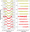 |
Fig. 1 Transits from the DK telescope. Left panel: light curves of 11 transits (10 complete and one partial) of HATS-2 b observed with the Danish 1.54 m telescope, shown in chronological order. They are plotted against the orbital phase and are compared to the best-fitting models. Labels indicate the observation date and the filter (Bessell I and R) that was used for each data set. Starspot anomalies are visible in all the light curves. Right-hand panel: the residuals of each fit. |
2.3 TESS space telescope
The PDCSAP (Pre-search Data Conditioning Simple Aperture Photometry; Smith et al. 2012; Stumpe et al. 2014) light curve of HATS-2 from both Sector 10 and 36 of the NASA TESS mission was downloaded through the Python package lightkurve (Lightkurve Collaboration et al. 2018), from the Mikulski Archive for Space Telescopes (MATS). Using the same Python package, we downloaded also raw PDCSAP data from Sector 63, for which the detrending was performed thanks to the wotan Python package (Hippke et al. 2019). The detrended data from each sector are shown in Fig. 3. Continuous observations of the target star were obtained for two periods of roughly 25 days (from 2019 March 28 to 2019 April 21) and 24 days (from 2021 March 08 to 2021 March 31) for Sectors 10 and 36, respectively. For Sector 63, the target star was observed for a period of 25 days (from 2023 March 11 to 2023 April 05) collecting, however, more transits. In fact, the data from Sector 10 and Sector 36 contain fifteen transits of HATS-2 b, while Sector 63 contains eighteen transits. The sub-optimal quality of TESS data is due to the relative faintness of the HATS-2 star (V = 13.6 mag), which is at the limit of the working magnitude of TESS. Nevertheless, several transits show clear anomalies, see Figs. A.1–A.3.
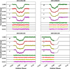 |
Fig. 2 Light curves of four (three complete and one partial) transits of HATS-2 b simultaneously observed in four optical bands (Sloan g′, r′, i′, z′) with the GROND multi-band camera at the MPG 2.2 m telescope. They are shown in date order. The light curves in the top panels are from Mohler-Fischer et al. (2013), while those in the bottom panels are from this work. Starspot anomalies are visible in the first three data sets. The light curves are plotted against the orbital phase and are compared to the best-fitting models. The residuals of the fits are shown at the base of each panel. |
3 Light curves analysis
Since many of our obtained light curves contained anomalies that could be connected to starspot complexes occulted by the exoplanet HATS-2b during its transits in front of its parent star, we had to model them with codes that are optimised against the presence of starspots and plages. Previous works showed that the presence of starspot anomalies not properly modelled could cause measures that mimic TTVs (Oshagh et al. 2013), or an anomalous planetary radius towards the bluest wavelengths (Oshagh et al. 2014).
The quality of our light curves is good enough to let us hypothesise that the anomalies are caused by starspot-occultation events (this is also supported by the spectral class of the host star) but not good enough to make assumptions about the fine structures of the starspots (as discriminate between single spots or groups of spots). So, it is normal practice to model the anomalies assuming one or more circular spots. As in the previous works of our series (e.g. Mancini et al. 2013, 2014b, 2015, 2017), we decided to use the PRISM and GEMC codes1 (Tregloan-Reed et al. 2013, 2015), which let us model the light curves fitting both the transit and one or several spot-crossing events simultaneously thanks to a bayesian approach and the use of genetic algorithms (Ter Braak 2006). PRISM+GEMC is set to use the quadratic Limb-Darkening (LD) law and, assuming a circular orbit, can model a light curve fitting for the following parameters: the sum of the fractional radii of the star and planet2, r* + rp, the ratio of the radii, ![$\[k=\frac{R_{\mathrm{p}}}{R_{\star}}=\frac{r_{\mathrm{p}}}{r_{\star}},\]$](/articles/aa/full_html/2024/05/aa47872-23/aa47872-23-eq1.png) the orbital inclination, i, the LD coefficients, u1 and u2, the time of mid-transit, T0, the longitude and latitude (ϕ, θ) of the centre of the starspot and, finally, the radius, rs, and the contrast, ρ, of the starspot (i.e. the ratio of the surface brightness of the starspot to that of the surrounding photosphere).
the orbital inclination, i, the LD coefficients, u1 and u2, the time of mid-transit, T0, the longitude and latitude (ϕ, θ) of the centre of the starspot and, finally, the radius, rs, and the contrast, ρ, of the starspot (i.e. the ratio of the surface brightness of the starspot to that of the surrounding photosphere).
We used PRISM+GEMC to analyse all the ground-based data sets presented in the previous section, four transits from Sector 10 of the TESS mission, six transits from Sector 36, and six transits from Sector 63. We also reanalysed the two light curves that were recorded with the MPG 2.2 m telescope by Mohler-Fischer et al. (2013). From now on, we will refer to the TESS transits from Sectors 10 and 36 using a numerical identification between 1 and 15 for both sectors, while those from Sector 63 between 1 and 18. The transit events have been labelled following a chronological order, in other words, from the left to the right referring to Fig. 3. All the transit events, with their relative id number, are shown in Fig. 3.
By using PRISM+GEMC, we analysed the light curves #2, #4, #14, and #15 from Sector 10 and those from #6 to #11 from Sector 36, as they show clear transit anomalies. Regarding Sector 63, the curves that presented anomalies were the ones labelled: #3, #9, #11, #13, #14, and #15. We used 1000 generations and 256 chains during the burn-in stage, and 128 chains during the burn-out stage (for details see Tregloan-Reed et al. 2015). The uncertainties have been adjusted by multiplying each data set by the square root of the reduced chi-squared value obtained during the burn-in stage, that is ![$\[\beta=\left(\chi_{\text {red }}^2\right)^{1 / 2}.\]$](/articles/aa/full_html/2024/05/aa47872-23/aa47872-23-eq2.png)
We always fitted for a single starspot on the stellar disc, except for the cases of the 2012 June 1st g′ transit from the MPG 2.2 m, the 2015 January 25 g′ r′ i′ transits from the MPG 2.2 m, and the #9 TESS transit from Sector 36. The results of the fit are listed in Tables 2 and E.1, while the best-fitting models and their residuals are shown in Figs. 1 and 2, and in the Appendix (see Figs. A.1–A.5). Regarding Sector 63, unbinned and 10 min cadence binned data were available, and we decided to fit both for the curves that contained anomalies. In Figs. A.4 and A.5, the reader can observe both the unbinned and 10 min cadence binned data. The results were always consistent for the two different data sets and so we kept the ones that gave us the smaller uncertainties regarding the starspot properties. It is worth underlining that if we did not have the unbinned data as a comparison, deciding to keep results from binned data would have been dangerous as the binning process could introduce systematics and bias the results (e.g. Kipping 2010).
The values in Table 2 refer to the median values of the posterior-probability-density (PDF) function of the parameters and not to the best-fitting parameters. The large uncertainties in the starspot parameters are caused by the fact that in some cases (as for the 2017 May 30 transit) the anomalies amplitudes are too small (<2 mmag) and in other cases (TESS) the scatter in the light curves is too high (>2 mmag). In both scenarios, PRISM/GEMC can find reasonable starspot parameters but the associated error bars are large because a wide range of solutions could produce such small or unclear anomalies.
The other light curves of Sector 10 and 36, which do not show detectable anomalies, have been analysed by using JKTE-BOP (Southworth 2008), which is faster than PRISM+GEMC and can fit the same photometric parameters except for the starspot parameters. The results are listed in Table E.1 and the reader can inspect the best-fitting models in Figs. A.6 and A.7. For Sector 63, all the light curves (unbinned data) were analysed by using PRISM+GEMC. The results are listed in Table E.1 and shown in Fig. A.8.
Due to the large scatter in TESS data, it is convenient to fit multiple transits simultaneously, as pointed out by several authors (e.g. Mancini et al. 2016; Southworth et al. 2022). This approach leads to more precise measurements of the sum and ratio of the radii, the inclination and, above all, the mid-transit times. In particular, we chose to perform a fit for each of the four periods of continuous observations. We considered transits from #1 to #8 and from #9 to #15 for the data in both Sectors 10 and 36, see Fig. 3. We applied the same reasoning to the Sector 63 TESS data. In particular, we chose to perform four different fits considering in order: (i) transits from #1 to #5, (ii) from #6 to #9, (iii) from #10 to #14, and (iv) from #15 to #18. Moreover, we fixed the non-linear LD coefficient, while the linear one has been set as a free parameter. Uncertainties were estimated using a Monte Carlo method. The final values of the parameters were estimated by a weighted mean of all the fits of all the light curves that are listed in Table E.1.
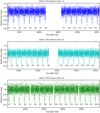 |
Fig. 3 Photometric monitoring of HATS-2 by the TESS space telescope. Top panel: data from Sector 10. Middle panel: data from Sector 36. Bottom panel: data from Sector 63. Fifteen transit events of HATS-2 b were detected by TESS in Sector 10 and 15 in Sector 36, while 18 transit events were detected in Sector 63. |
Starspot parameters derived from the PRISM+GEMC fits of the transit light curves.
Median values and 68% confidence intervals of the physical and orbital properties of the HATS-2 system, found using JKTABSDIM.
4 Physical and starspot properties of the HATS-2 exoplanetary system
4.1 Stellar and planetary parameters
To estimate the main physical parameters of the HATS-2 system, we used the code jktabsdim3 (Southworth et al. 2009). The code makes use of the spectroscopic parameters, the stellar radial-velocity (RV) semi-amplitude (K* = 268.9 ± 29.0 m s−1; Mohler-Fischer et al. 2013) and a set of theoretical stellar models. In particular, JKTABSDIM uses tabulations from the Claret (Claret 2004), Y2 (Demarque et al. 2004), and Padova (Girardi et al. 2000) models. JKTABSDIM works in such a way that the velocity amplitude of the planet is iteratively modified to maximise the agreement between the best additional constraint derived from different theoretical models and the observed values of the stellar density from transit, effective temperature and metallicity (Teff = 5227 ± 95 and [Fe/H] = 0.15 ± 0.05; Mohler-Fischer et al. 2013). A wide range of possible ages for the parent star is also considered during this process. The code returns different estimates for each of the output parameters, one for each set of theoretical models. The unweighted means are considered the final values of the parameters. The systematic uncertainties, which were caused by the use of theoretical models, were estimated, while the statistical uncertainties were propagated from the uncertainties of the input parameters. It is worth to underline that jktabsdim does not use Gaia parallax, any apparent magnitudes, or interstellar extinction. As a consistency check, we calculated the distance to the system using our measurements of the stellar radius and effective temperature, apparent magnitudes in the optical (BV) and in the infrared (2MASS JHK), and the surface brightness relations from Kervella et al. (2004). An interstellar reddening of E(B − V) = 0.08 ± 0.03 mag was needed to align the distances in the optical and infrared passbands, and the distance found in the K-band is 332 ± 9 pc. The Gaia DR3 distance of 337 ± 2 pc is in good agreement with this value.
The final values of the parameters are listed in Table 3 and are in good agreement with those from Mohler-Fischer et al. (2013). The only parameter that differs (although only at ~1.5 σ) is the planetary radius, which appears smaller in size. It is also possible to compare the final values with the ones obtained considering a weighted mean of the results of only the curves that do not present anomalies. The difference between these values can be considered as a first-order approximation of the systematic error introduced by the modelling of the starspots, which due to the low data quality, is within the 1-sigma uncertainties. In this way we derived that the systematic error is 0.85 % regarding the sum of the radii and 1.3 % regarding the ratio of the radii.
4.2 Starspot analysis
Having modelled the HATS-2 transit light curves containing starspot anomalies with the PRISM-GEMC codes, we were able to derive the best-fitting values for the position of the starspots on the stellar disc, beyond their angular size and contrast. These estimations are reported in Table 2, in whose last column the reader can also find the starspot-temperature values, which were derived considering the stellar photosphere and starspots as black bodies and using equation 1 from Silva (2003), that is
![$\[\rho=\frac{B_v\left(T_{\text {spot }}\right)}{B_v\left(T_{\text {eff }}\right)}=\frac{\exp \left(h v / k_{\mathrm{B}} T_{\text {eff }}-1\right)}{\exp \left(h v / k_{\mathrm{B}} T_{\text {spot }}-1\right)},\]$](/articles/aa/full_html/2024/05/aa47872-23/aa47872-23-eq3.png) (1)
(1)
where ν is the central frequency of each filter band4, h is the Planck constant, while kB is the Boltzmann constant. All the values are consistent with starspots cooler than the stellar photosphere and lie between 4000 and 5000 K, within the uncertainties.
The only exception is related to the first anomaly on the g′ light curve of the transit observed on 2012 June 1st, which was identified by Mohler-Fischer et al. (2013) as a plage (see the top right-hand panel in Fig. 2). In the case of the Sun, plages are usually visible through H-α or calcium (Ca) K line wavelengths by using appropriate filters. In K-type stars, such as HATS-2, the Ca II lines are much stronger than the H-α ones and fall in the wavelength transmission range defined by the g′ filter, λ = 478.8 ± 137.9 nm. We, therefore, agree with the interpretation of Mohler-Fischer et al. (2013) that the anomaly could be caused by a plage connected with the following starspot.
In general, we noted that the angular sizes of the starspots vary from a minimum of 2.9° to a maximum of 40°−50°. Considering that an angular radius of 90° covers half of the stellar hemisphere, the starspots we have found cover from a minimum of 1.6% to a maximum of 20-30% of the stellar disc. As in the case of, e.g. TrEs-1 and WASP-19, our measurements are similar to those found for other G-type and K-type stars (Rabus et al. 2009; Mancini et al. 2013) and are in good agreement with the sizes of very large sunspots (Sun et al. 2015). However, we stress that some of the starspots, which we have detected and modelled with circular shapes, might actually be a group of starspots, according to the Zurich and McIntosh classifications (McIntosh 1990).
Since starspots are darker in the ultraviolet than in the infrared and we observed transits through different filters, we can check if the starspot contrast varies as expected as a function of the wavelength. In Fig. 4 we compare the starspot contrasts estimated by PRISM+GEMC and reported in Table 2 with theoretical expectations. Using ATLAS9 atmospheric models (Kurucz 1979), we modelled a stellar photosphere of 5227 K and starspots with five different temperature 4200 K, 4400 K, 4600 K, 4850 K and 4980 K. Although the error bars of the starspot contrasts are quite large, the trend in each panel of Fig. 4 is that for which the starspots are brighter in the redder passbands than in the bluer one, for both all three complete simultaneous GROND multi-band observations and the two-colours observations with the Danish telescope.
4.3 Spin–orbit alignment
We investigated the possibility that some of the observed starspot-crossing events have been caused by the same starspot because, then, as explained in Sec. 1, the spin–orbit alignment of the planetary system can be derived.
Mohler-Fischer et al. (2013) already argued that the anomalies observed during the 2012 February 28 and 2012 June 1st transits could have been caused by the same starspot. Studying the values reported in Table 2, we note that, for these two transits, the differences in the starspot latitudes in all the GROND bands fall within 1σ but their angular sizes are not similar. Hence, it is possible that we are dealing with a starspot complex that evolved following the Zurich classification. However, the two transits are separated by 94 days and, using empirical laws, Mohler-Fischer et al. (2013) estimated that a group of starspots with this size could have a lifetime of -130 days. With these caveats, the authors estimated a sky-projected obliquity of 8° ± 8° and a rotational period of 31 ± 10 days.
Using the new data presented in this work, we identified eleven consecutive starspot-crossing events, separated by less than 5 days, and for which the relative latitudes and angular sizes differences fall within 1σ, referring to the values listed in Table 2. 10 out of 11 events have been identified in the TESS photometric data. Of particular interest are the consecutive transits that we labelled with #7 and #8 from TESS Sector 36 (see Fig. 5). Investigating the light curves (see Fig. A.2), we note that the anomalies that appear in the transits #7 and #8 have similar amplitudes and duration, whereas the time of the maximum of the anomalies changes with the increase of the orbital phase. These facts suggest that the anomalies are due to the same starspot rotating around the surface of the star.
This hypothesis is also supported by the modelling results from PRISM/GEMC. Indeed, the best-fitting circular starspots for the transit events #7 and #8 have similar sizes and contrasts (see Table 2). The transit designed as number #6 also supports this hypothesis, although its small size does not allow us to constrain the size of the starspot with the required accuracy.
The other TESS consecutive transit events were identified as #14 and #15 from Sector 10 (Fig. A.1), as #9, #10, and #11 from Sector 36 (Fig. A.3), and as #13, #14, and #15 from Sector 63 (Fig. A.4).
The two consecutive starspot-crossing events, which were identified using our data from ground-based telescopes, are those from the Danish 1.54 m telescope observed on 2019 May 19 and 2019 May 23 (see Fig. 1).
Using the values listed in Table 2, it is possible to calculate the values of the sky-projected obliquity, λ, and the stellar rotational period Prot for each of the identified events by using the following equations:
![$\[|\lambda|=\arctan \left(\left|\frac{\sin \theta_2-\sin \theta_1}{\cos \theta_2 \sin \phi_2-\cos \theta_1 \sin \phi_1}\right|\right),\]$](/articles/aa/full_html/2024/05/aa47872-23/aa47872-23-eq4.png) (2)
(2)
![$\[P_{\text {rot }}=\frac{2 \pi \Delta t}{\sqrt{D}},\]$](/articles/aa/full_html/2024/05/aa47872-23/aa47872-23-eq5.png) (3)
(3)
![$\[\begin{aligned}D= & 2\left(1-\sin \theta_1 \sin \theta_2-\cos \theta_1 \cos \theta_2 \sin \phi_1 \sin \phi_2\right) \\& +\cos ^2 \theta_2\left[\sin ^2 \phi_2-1\right]+\cos ^2 \theta_1\left[\sin ^2 \phi_1-1\right],\end{aligned}\]$](/articles/aa/full_html/2024/05/aa47872-23/aa47872-23-eq6.png) (4)
(4)
where θ1,2 and ϕ1,2 are the latitudes and longitudes of the two consecutive starspots and Δt is the time interval between the two starspot-crossing events. The quantity ![$\[\sqrt{D}\]$](/articles/aa/full_html/2024/05/aa47872-23/aa47872-23-eq7.png) represents the arc length on the stellar photosphere between the two positions of the starspot. The mathematical derivation of these equations is given in the Appendix. The values of λ and Prot are reported in Table 4 for each event. The large uncertainties associated with the |λ| and Prot values derived from some of the TESS light curves must be once again intended, as explained in Sec. 3, as a consequence of the poor quality (high scatter) of the data. Our final estimations were computed by performing a weighted mean, obtaining |λ| = 2°.72 ± 17o.84 and Prot = 22.46 ± 5.20 days. This value is consistent with the value of Prot, TESS = 21.44 days, obtained with a FAP < 0.1% (false alarm probability) performing a GLS (Generalised Lomb-Scargle Periodgram, VanderPlas 2018) analysis of the SAP flux from all the three sectors of the TESS Mission, see Fig. C.1. The estimation of the sky-projected obliquity resulted consistent with zero degrees and, therefore, with a well-aligned system. It is represented in Fig. 6 as a function of the parent-star effective temperature, together with a sample of values taken from the TEPCat catalogue5.
represents the arc length on the stellar photosphere between the two positions of the starspot. The mathematical derivation of these equations is given in the Appendix. The values of λ and Prot are reported in Table 4 for each event. The large uncertainties associated with the |λ| and Prot values derived from some of the TESS light curves must be once again intended, as explained in Sec. 3, as a consequence of the poor quality (high scatter) of the data. Our final estimations were computed by performing a weighted mean, obtaining |λ| = 2°.72 ± 17o.84 and Prot = 22.46 ± 5.20 days. This value is consistent with the value of Prot, TESS = 21.44 days, obtained with a FAP < 0.1% (false alarm probability) performing a GLS (Generalised Lomb-Scargle Periodgram, VanderPlas 2018) analysis of the SAP flux from all the three sectors of the TESS Mission, see Fig. C.1. The estimation of the sky-projected obliquity resulted consistent with zero degrees and, therefore, with a well-aligned system. It is represented in Fig. 6 as a function of the parent-star effective temperature, together with a sample of values taken from the TEPCat catalogue5.
Considering that HATS-2 has Teff = 5227 ± 95 K, our result is in agreement with the trend for which the orbits of the hot Jupiters hosted around cool dwarf stars tend to present a low obliquity (Winn et al. 2010). Moreover, this can be an indication that HATS-2b has reached its actual position through a Type II migration, or that tidal interactions with its parent star damped a non-zero obliquity caused by Lidov-Kozai oscillations induced by a distant companion (Raymond & Morbidelli 2022). The second scenario is preferable as HATS-2 is a quite old (~7 Gyr) K-type star, so both the age and the convective envelope enhance the tidal dissipation efficiency. The analysis of the TTVs, which is discussed in the next section, will provide other insights to discriminate between the two formation scenarios.
Knowing the rotational period of the parent star and using (υ sin i*) from Mohler-Fischer et al. (2013), we determined the sine of inclination of the stellar-rotation axis by means of
![$\[\sin i_{\star}=P_{\text {rot }} \frac{\left(v \sin i_{\star}\right)}{2 \pi R_{\star}}=0.76 \pm 0.31.\]$](/articles/aa/full_html/2024/05/aa47872-23/aa47872-23-eq8.png) (5)
(5)
Then, using the following formula (Winn et al. 2007)
![$\[\cos \psi=\cos i \cos i_{\star}+\sin i \sin i_{\star} \cos \lambda,\]$](/articles/aa/full_html/2024/05/aa47872-23/aa47872-23-eq9.png) (6)
(6)
we derived the true orbital obliquity of HATS-2b, which resulted to be ψ = 38°.49 ± 27°. 13. This measurement excludes that HATS-2 is in a pole-on configuration.
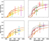 |
Fig. 4 Variation in the starspot contrast with wavelength. The vertical bars represent the errors in the measurements and the horizontal bars show the FWHM transmission of the passbands used. In the upper panels, the colour of the data points is in agreement with Fig. 2. In the top left panel, the data taken on 2012 February 28 with the GROND multi-band camera are represented together with the ATLAS9 (Kurucz 1979) stellar atmospherical models computed considering a stellar surface at 5227 K and a starspot at 4200 and 4400 K. In the top right panel, the data taken on 2012 June 1st with the GROND multi-band camera are represented together with the ATLAS9 stellar atmospherical models computed considering a stellar surface at 5227 K and a starspot at 4600, 4850, and 4980 K. In the bottom panels, the points represent the contrast values obtained using the Danish 1.54 m transits (as explained in the plot legend), while the curves are the same ATLAS9 models used in the upper panels. |
 |
Fig. 5 Representation of the stellar disc, starspot position, and transit chord for the two consecutive transit events, #7 (left panel) and #8 (right panel) with starspot crossings, obtained using PRISM/GEMC. The grey scale of each starspot is related to its contrast. The starspot properties refer to the best-fitting models in Fig. A.2 (see Appendix). |
All the spot-crossing events identified over two transits in this work.
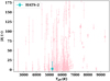 |
Fig. 6 Sky-projected obliquity as a function of the host stars’ effective temperature for an ensemble of exoplanetary systems. The star is the value of the sky-projected obliquity of the HATS-2 system found in this work, while the dots are the values from the TEPCAT catalogue. |
Times of mid-transit for HATS-2b and relative O–C residuals.
5 Transit timing variations
Thanks to the analysis of the light curves presented in the previous sections, we have a set of mid-transit times, which are listed in Table 5. The values derived from the GROND light curves refer to a weighted mean of the T0 values obtained in each of the four optical filters, while the values derived from the TESS light curves refer to the result of the eight simultaneous fits with JKTEBOP.
We also used a series of light curves from the ExoClock database (Kokori et al. 2022)6. In particular, we selected the most well-sampled (i.e. with well-sampled ingress, plateau and egress) and high-quality (i.e. low scatter; see the last column of Table 1) light curves from those presented by Edwards et al. (2021) and Kokori et al. (2023). In detail, we selected three light curves collected at the Deep Sky Chile Observatory on 2021 January 10, 2021 April 11, and 2021 April 15 (Kokori et al. 2023), and one at the Sliding Spring Observatory on 2021 February 22 (Edwards et al. 2021).
We also considered two unpublished light curves once more collected by amateur astronomers within the ExoClock collaboration; one was again observed with the Deep Sky Chile 40 cm telescope, while the other with the Hakos Astro Farm 50 cm telescope7.
All these extra light curves were fitted with the same procedures presented in the previous sections thanks to the JKTEBOP and PRISM+GEMC codes. The best-fitting models are presented in Fig. D.1 together with the detrended light curves. The results are listed in Table D.1. In the end, our final ensemble of mid-transit times covers a time baseline extending over more than 10 yr. It is, therefore, possible to refine the ephemerides by considering various models for fitting the timings.
We set the middle transit of the second half of the Sector 10 TESS data to be the zeroth epoch because most of its light curve does not show the presence of anomalies connected to starspots within the experimental uncertainties and has been estimated by a simultaneously fit with the ‘neighbour’ transits.
We considered two different data sets: (a) fitting only GROND, DFOSC and TESS data without ExoClock times, and (b) fitting all the data listed in Table 5. The first model that we tried is a simple straight line, ![$\[T_0^{\text {lin }}=\kappa_0+\kappa_1 \times E\]$](/articles/aa/full_html/2024/05/aa47872-23/aa47872-23-eq10.png) , which represents a linear ephemeris. In case (a), we obtained
, which represents a linear ephemeris. In case (a), we obtained
![$\[T_0^{\text {lin }}=\mathrm{BJD}_{\mathrm{TDB}} 58591.08501(11)+1.35413385(9) \times E,\]$](/articles/aa/full_html/2024/05/aa47872-23/aa47872-23-eq11.png) (7)
(7)
![$\[T_0^{\text {lin }}=\mathrm{BJD}_{\mathrm{TDB}} 58591.084931(96)+1.35413379(8) \times E.\]$](/articles/aa/full_html/2024/05/aa47872-23/aa47872-23-eq12.png)
Here, E represents the epoch of the transit and the bracketed quantities indicate the uncertainties in the preceding digits. Variations of the order of minutes are evident from the O–C residuals of both of the two fits shown in Fig. 7. This means that the linear ephemeris is a good approximation but seems to not exactly reproduce the dynamic state of the system.
Since physical phenomena may hide in these variations, we also tried to fit the data with
a quadratic polynomial that represents a quadratic ephemeris and could be connected to a tidal-decay scenario
![$\[T_0^{\text {quad }}=\kappa_0+\kappa_1 \times E+\kappa_2 \times E^2,\]$](/articles/aa/full_html/2024/05/aa47872-23/aa47872-23-eq13.png) (9)
(9)a sinusoidal function that could be seen as a linear ephemeris periodically perturbed with an amplitude ATTV, a period PTTV = 2π/Ω, and a phase φ. This ephemeris could be connected to an apsidal precession scenario or the presence of a planetary or sub-stellar companion (e.g. a brown dwarf)
![$\[T_0^{\sin }=\kappa_0+\kappa_1 \times E+A \sin (\Omega E+\varphi).\]$](/articles/aa/full_html/2024/05/aa47872-23/aa47872-23-eq14.png) (10)
(10)
All the fits were performed using the lmfit (Newville et al. 2014) Python package. The results are listed in Table 6 and their O–C residuals versus the best-fitting linear model are represented in Fig. 7, for both scenarios. The sinusoidal and quadratic ephemeris seems to fit better the data with respect to the linear one as confirmed by statistical indicators, such as the Reduced Chi-Squared χred, the Bayesian information criterion (BIC) and the Akaike information criterion (AIC), which are, respectively, defined as
![$\[\chi_{\text {red }}^2=\frac{\chi^2}{N_{\text {dof }}}=\frac{\chi^2}{N-j},\]$](/articles/aa/full_html/2024/05/aa47872-23/aa47872-23-eq15.png) (11)
(11)
![$\[\mathrm{BIC}=N \ln \left(\frac{\chi^2}{N}\right)+N_{\Theta} \ln N,\]$](/articles/aa/full_html/2024/05/aa47872-23/aa47872-23-eq16.png) (12)
(12)
![$\[\mathrm{AIC}=N \ln \left(\frac{\chi^2}{N}\right)+2 N_{\Theta},\]$](/articles/aa/full_html/2024/05/aa47872-23/aa47872-23-eq17.png) (13)
(13)
where N is the number of data points and NΘ is the number of parameters of the best-fitting model. Ndof is the number of degrees of freedom and usually is set as the number of data points N minus the number of free parameters NΘ. The ![$\[\chi_{\text {red }}^2\]$](/articles/aa/full_html/2024/05/aa47872-23/aa47872-23-eq18.png) , BIC and AIC values for each of the considered ephemeris models and groups of data are listed in Table 7.
, BIC and AIC values for each of the considered ephemeris models and groups of data are listed in Table 7.
All the ![$\[\chi_{\text {red }}^2,\]$](/articles/aa/full_html/2024/05/aa47872-23/aa47872-23-eq19.png) values listed in Table 7 are larger than unity. This is not a sign of a bad fit but is in line with our previous TTV analysis, (see e.g. Mancini et al. 2022b and references within). As pointed out in various works (e.g. Patra et al. 2017; Mancini et al. 2022b), the difference between the BIC and AIC values of two models, η = ΔBIC and ξ = ΔAIC, are good statistical indicators. In particular, η > 10 and a ξ > 10 indicate that the evidence favouring the lower BIC model against the other is very strong.
values listed in Table 7 are larger than unity. This is not a sign of a bad fit but is in line with our previous TTV analysis, (see e.g. Mancini et al. 2022b and references within). As pointed out in various works (e.g. Patra et al. 2017; Mancini et al. 2022b), the difference between the BIC and AIC values of two models, η = ΔBIC and ξ = ΔAIC, are good statistical indicators. In particular, η > 10 and a ξ > 10 indicate that the evidence favouring the lower BIC model against the other is very strong.
First, we focus on the comparison between the linear and the quadratic ephemeris models. Without the ExoClock data, the quadratic model is favoured by a η = 9.6 and a ξ = 10.7, so we are at the limit of the statistical significance. Adding the Exo-Clock data, the quadratic model is favoured by a η = 15.1 and a ξ = 16.4. So, the tidal-decay scenario seems to be highly preferred with respect to a simple linear-ephemeris scenario and this makes HATS-2 a good candidate in the context of the search for secular timing variations in hot Jupiters (Hagey et al. 2022). Focusing now on the second scenario results, by using the values listed in Table 6 and the following formula (Patra et al. 2017):
![$\[\frac{1}{2} \frac{\mathrm{d} P}{\mathrm{~d} E} E^2=-\frac{27 \pi}{4 Q_{\star}^{\prime}} \frac{M_{\mathrm{p}}}{M_{\star}}\left(\frac{R_{\star}}{a}\right)^5 P E^2,\]$](/articles/aa/full_html/2024/05/aa47872-23/aa47872-23-eq20.png) (14)
(14)
we derived a ![$\[\frac{\mathrm{d} P}{\mathrm{~d} E}=-(5.48 \pm 2.48) \times 10^{-10}\]$](/articles/aa/full_html/2024/05/aa47872-23/aa47872-23-eq21.png) days per orbital cycle, and therefore the period derivative is
days per orbital cycle, and therefore the period derivative is ![$\[\dot{P}=\frac{1}{P} \frac{\mathrm{d} P}{\mathrm{~d} E}=-15.7\]$](/articles/aa/full_html/2024/05/aa47872-23/aa47872-23-eq22.png) ± 3.5 ms yr−1, consistent with an orbital period that shrink to zero in a time within
± 3.5 ms yr−1, consistent with an orbital period that shrink to zero in a time within ![$\[\frac{P}{\mathrm{~d} P / \mathrm{d} t}=\frac{P^2}{\mathrm{~d} P / \mathrm{d} E}=7.5 \pm 1.7\]$](/articles/aa/full_html/2024/05/aa47872-23/aa47872-23-eq23.png) Myr. This is reasonable for a planet that orbits around its host star with a semi-major axis ≃ 2 times the Roche radius and so close to tidal disruption. Using Eq. (14), we also derived a limit to the modified stellar tidal dissipation quality factor of
Myr. This is reasonable for a planet that orbits around its host star with a semi-major axis ≃ 2 times the Roche radius and so close to tidal disruption. Using Eq. (14), we also derived a limit to the modified stellar tidal dissipation quality factor of ![$\[Q_{\star}^{\prime}\]$](/articles/aa/full_html/2024/05/aa47872-23/aa47872-23-eq24.png) > (1.99 ± 0.26) × 104; this result is based on the 95 per cent confidence lower limits on
> (1.99 ± 0.26) × 104; this result is based on the 95 per cent confidence lower limits on ![$\[\dot{P}\]$](/articles/aa/full_html/2024/05/aa47872-23/aa47872-23-eq25.png) , while the uncertainties come from propagating the errors in Mp/M* and R*/a. This result is consistent with theoretical works such that by Ahuir et al. (2021). In Fig. 8, we plot the obtained limit as a function of stellar age and planetary equilibrium temperature, together with the values obtained for other systems hosting hot Jupiters that can be considered good candidates to study orbital decay. These are: KELT-16 (Mancini et al. 2022b), HATS-18 (Southworth et al. 2022), WASP 18 and WASP 19 (Rosário et al. 2022), WASP-12 (Wong et al. 2022), WASP-4 (Turner et al. 2022), WASP-103 (Barros et al. 2022), and TrES-1, TrES-5 and HAT-P-19 (Hagey et al. 2022). The stellar ages were taken from Bonomo et al. (2017). In Hagey et al. (2022) only the orbital period derivates were presented, so we had to compute the
, while the uncertainties come from propagating the errors in Mp/M* and R*/a. This result is consistent with theoretical works such that by Ahuir et al. (2021). In Fig. 8, we plot the obtained limit as a function of stellar age and planetary equilibrium temperature, together with the values obtained for other systems hosting hot Jupiters that can be considered good candidates to study orbital decay. These are: KELT-16 (Mancini et al. 2022b), HATS-18 (Southworth et al. 2022), WASP 18 and WASP 19 (Rosário et al. 2022), WASP-12 (Wong et al. 2022), WASP-4 (Turner et al. 2022), WASP-103 (Barros et al. 2022), and TrES-1, TrES-5 and HAT-P-19 (Hagey et al. 2022). The stellar ages were taken from Bonomo et al. (2017). In Hagey et al. (2022) only the orbital period derivates were presented, so we had to compute the ![$\[Q_{\star}^{\prime}\]$](/articles/aa/full_html/2024/05/aa47872-23/aa47872-23-eq26.png) limits via Eq. (14); the planetary and stellar parameters have been taken from the literature (i.e. Stassun et al. 2017; Maciejewski et al. 2016; Johnson et al. 2009; Hartman et al. 2011). The results show a correlation between the derived tidal quality factor and the planetary equilibrium temperature, in agreement with Eq. (14). In this context, the value derived for HATS-2 occupies the right place in the diagram of the tidal quality factor versus stellar age and equilibrium temperature. The relation between the stellar tidal quality factor and the stellar age is not clear and further observations may give new insights.
limits via Eq. (14); the planetary and stellar parameters have been taken from the literature (i.e. Stassun et al. 2017; Maciejewski et al. 2016; Johnson et al. 2009; Hartman et al. 2011). The results show a correlation between the derived tidal quality factor and the planetary equilibrium temperature, in agreement with Eq. (14). In this context, the value derived for HATS-2 occupies the right place in the diagram of the tidal quality factor versus stellar age and equilibrium temperature. The relation between the stellar tidal quality factor and the stellar age is not clear and further observations may give new insights.
Investigating Table 7, it is possible to observe that also a sinusoidal model can explain the data well. In fact, in both scenarios, the relative η and ξ are always smaller than 5. The sinusoidal model can be connected to the presence of apsidal precession induced by the tidal interactions between the planet and the host star (Ragozzine & Wolf 2009; Gimenez & Garcia-Pelayo 1983):
![$\[\mathrm{O}-\mathrm{C} \simeq-\frac{e P_{\mathrm{a}}}{\pi} \cos \omega=-\frac{e P_{\mathrm{a}}}{\pi} \cos \left(\omega_0+\frac{\mathrm{d} \omega}{\mathrm{d} E} E\right),\]$](/articles/aa/full_html/2024/05/aa47872-23/aa47872-23-eq27.png) (15)
(15)
![$\[\frac{\mathrm{d} \omega}{\mathrm{d} E} \simeq 15 \pi k_{2, p} \frac{M_{\star}}{M_{\mathrm{p}}}\left(\frac{R_{\mathrm{p}}}{a}\right)^5,\]$](/articles/aa/full_html/2024/05/aa47872-23/aa47872-23-eq28.png) (16)
(16)
where Pa indicates the sidereal period, ω the argument of the periastron, k2,p is the planet’s Love number and dω/dE the precession rate. Plugging the values listed in Table 6 into Eq. (16), we obtained a value of k2,p greater than 1.5 that has no physical meaning. The other physical explanation is the presence of a third body in the system (Agol et al. 2005). However, modelling TTVs induced by a third body is a highly degenerate problem and the quality of our data and the temporal coverage are not good enough to face it. In any case, future and systematic recordings of new mid-transit times will certainly give useful insights to entangle the problem. Figure 7 tells us that it should be possible to discriminate between the quadratic and the sinusoidal model by exploiting new transit measures in the next 2 yr.
Best-fit parameters of the ephemeris models for the HATS-2b mid-transit time residuals.
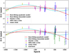 |
Fig. 7 Top panel: O–C residuals for HATS-2b in the case (a), superimposed with the best-fitting linear ephemeris model (black line), the best-fitting quadratic ephemeris model (red line) and the best-fitting cosinusoidal ephemeris model (cyan line). The purple points represent the times derived from the Danish 1.54 m telescope observations, the yellow points the times derived from the MPG/ESO 2.2 m telescope data, and the blue points the times derived from TESS data. Bottom panel: same as the top panel but for case (b), i.e. also considering the data from the ExoClock database, which are represented as green points. |
Goodness of fit of the three ephemeris models.
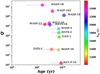 |
Fig. 8 Stellar tidal quality factor as a function of stellar age for HATS-2 and an ensemble of host stars. These stars were selected considering systems where tidal decay has been observed or is a possible explanation for the observed TTVs (Hagey et al. 2022; Rosário et al. 2022; Wong et al. 2022; Mancini et al. 2022b; Barros et al. 2022). |
6 Variation in the planetary radius with wavelength
Due to their proximity to their parent star, hot Jupiters are strongly irradiated and their spectra are expected to show several absorption features at optical wavelengths. Some of the features that are usually detected in the optical bands include sodium (~590 nm), potassium (~770 nm) and water vapour (~950 nm). In several cases, Rayleigh scattering at bluer wavelengths has been found as well as the presence of strong absorbers, such as gaseous titanium oxide (TiO) between 450 and 800 nm.
The transit depth is a parameter that depends on the wavelength and, therefore, on the possible absorption of the chemical species present in the exoplanetary atmosphere. Multi-colour photometry can be a useful tool for investigating how k changes with wavelength, probing in this way the chemical composition at the terminator of planetary atmospheres during transit events. Transmission photometry has, in general, a very low spectral resolution but is suitable for ground-based telescopes with smaller apertures and exoplanets orbiting faint stars. This type of study can be, therefore, useful to get information about the absorption behaviour of the exoplanetary atmosphere and guide more precise investigation via transmission spectroscopy, being the latter a most effective technique.
Using the light curves of the transits of HATS-2 b, which we obtained through observations at different passbands, we attempted to get a low-resolution transmission spectrum of HATS-2 b. Following a general approach, we run PRISM/GEMC for each of the ground-based light curves again to calculate the ratio of the radii in each passband, being the other photometric and starspots parameters fixed to the best-fitting values listed in Tables E.1 and 2. This yielded a set of k values which are directly comparable and whose error bars exclude common sources of uncertainty. In particular, for fixing the values of the LD coefficients, we calculated the weighted means of the values, based on their colour. As a last step, we averaged the ratio of the radii values taken with the same filters. The weighted mean was performed using the scatter in the light curves to set the size of the errorbar. In this way, we can be sure that the uncertainties will not be underestimated. We excluded the TESS light curves because the long-pass filter of TESS is just too wide (>500 nm) for our purposes. The results are:
![$\[\begin{aligned}& k_{g^{\prime}}=0.13192 \pm 0.00094 \\& k_{r^{\prime}}=0.13310 \pm 0.00063 \\& k_R=0.13258 \pm 0.00057 \\& k_{i^{\prime}}=0.13419 \pm 0.00067 \\& k_I=0.13405 \pm 0.00064 \\& k_{z^{\prime}}=0.13252 \pm 0.00083\end{aligned}\]$](/articles/aa/full_html/2024/05/aa47872-23/aa47872-23-eq29.png)
These values are shown in Fig. 9 and are compared with three 1D model atmospheres, which were obtained by Fortney et al. (2010).
In particular, the red line represents an equilibrium-chemistry spectrum, which was calculated for Jupiter’s gravity (25 m s−2) with a base radius of 1.25 RJup at the 10 bar level and at 1500 K. This model is dominated by H2/He Rayleigh scattering in the blue and pressure-broadened neutral atomic lines of sodium and potassium at 770 nm, and the opacity of TiO and VO molecules were included. The blue line represents a model similar to the previous one but the opacity TiO and VO were excluded. Another spectrum was computed from the latter by changing the intensity of Rayleigh scattering, which physically corresponds to considering different compositions and thicknesses of the external atmosphere layers. In particular, the dashed dark-green line was obtained by increasing the Rayleigh scattering by a factor of 10.
A variation in the planetary radius was found between the g′ and i′ bands. The variation is roughly 6.5 pressure scale heights8 but its significance is below the 2 σ level, which preserve us to claim any absorption detection.
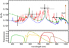 |
Fig. 9 Top panel: variation in the planetary radius, in terms of the planet-to-star radius ratio, with wavelength. The points are from the ground-based transit observations presented in this work (black from the MPG 2.2 m telescope and grey from the Danish 1.54m telescope). The vertical bars represent the errors in the measurements and the horizontal bars show the FWHM transmission of the passbands used. The observational points are compared with three synthetic spectra from Fortney et al. (2010, Red: equilibrium-chemistry; Blue: no TiO, VO opacity; Green: enhanced Rayleigh scattering). The same offset is applied to all four models to provide the best fit to the measurements. The size of 10 atmospheric pressure scale heights (10 × H) is shown on the right of the plot. Bottom panel: transmission curves for the Bessell I and R filters and the total efficiencies of the GROND filters. |
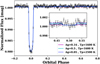 |
Fig. 10 HATS-2b phase curve obtained by phase-binning the data from Sectors 10, 36 and 63 of NASA’s TESS mission plotted against theoretical curves computed thanks to the batman Python package. |
7 Flux ratio of HATS-2 b from TESS phase curve
We investigated the possibility to measure the occultation depth, in other words the planet-to-star flux ratio Fp/F*, in the continuous time series data of TESS (see Fig. 3). For this purpose, we phased the data from every sector considering the best-fitting linear ephemeris found in the previous sections, Eq. (8), and binned them using a weighted sigma-clipping mean, which means that the data are iteratively kept or rejected in terms of standard deviation. The resulting phase curve is presented in Fig. 10, together with different theoretical phase curves generated thanks to the batman Python package (Kreidberg 2015). To simulate the occultation curves, batman needs two free parameters, the occultation depth and the occultation mid-time, and a series of fixed parameters as the mid-transit time, the ratio of the radii, the scaled stellar radius, the period, the eccentricity, and the inclination of the orbit. In turn, the occultation depth at visible wavelengths (such as the one at which the TESS bandpass is centred, ≃786 nm) can be connected to the planetary day-side temperature Tp and geometric albedo Ag (Kovacs et al. 2022):
![$\[\delta_{\mathrm{occ}} \simeq \delta_{\mathrm{refl}}+\delta_{\mathrm{th}} \simeq A_{\mathrm{g}}\left(\frac{R_{\mathrm{p}}}{a}\right)^2+k^2 \frac{B_v\left(T_{\mathrm{p}}\right)}{B_v\left(T_{\mathrm{eff}}\right)}\]$](/articles/aa/full_html/2024/05/aa47872-23/aa47872-23-eq30.png) (17)
(17)
where Bv is the Planck function. If we use Eq. (17) together with the values listed in Table 3 we can generate different theoretical light curves considering different scenarios and corresponding values for Ag and Tp. In particular, we considered three scenarios: (i) Ag = 0.16 and Tp = 1600 K, (ii) Ag = 0.5 and Tp = 1600 K, and (iii) Ag = 0.05 and Tp = 2500 K. The first scenario should be that closer to reality if we consider typical values of Ag found in the literature for hot Jupiters and a conservative atmospherical circulation. The second and third scenarios, instead, represent two opposite extremes. The second represents the situation where most of the light that we receive from the planet in the TESS bandpass is just reflected light; the third, instead, represents the case where the day-side temperature greatly exceeds the equilibrium temperature, for example, due to the presence of absorbers or tidal locking. In any case, none of the generated theoretical curves seems to be close to the phased TESS light curve for which a non-detection of the occultation is the most compatible scenario. Moreover, the uncertainty on the mean flux (unbinned) is close to 1 ppt (1000 ppm), which makes any tentative of measuring the occultation depth extremely difficult. In the end, as expected due to the faintness of the parent star, we did not report any detection of a secondary eclipse in the HATS-2 TESS photometry. This work and TESS photometry place an upper limit on the occultation depth of HATS-2b, δocc < 400 ppm.
8 Summary and conclusions
In this work, we studied the physical and orbital properties of the hot Jupiter HATS-2 b, a giant transiting exoplanet with Porb ≈ 1.35 days, and therefore, an interesting target to investigate in relation to a possible orbital-decay process. We reported the photometric monitoring of 13 new transit events of HATS-2 b, which were observed with two medium-class telescopes through six different optical passbands (see Figs. 1 and 2). The transits were observed using the defocusing technique, achieving a photometric precision of 0.6 mmag per observation in the best case. Two transits were simultaneously observed in four optical bands thanks to the GROND multi-band camera. In total, we collected 19 new light curves. We also considered the data from two other transits observed with GROND (Mohler-Fischer et al. 2013) and four published and two new light curves (see Fig. D.1) that were recorded by amateur astronomers within the ExoClock project. We also considered the photometric data collected by TESS and analysed 48 complete transits recorded by this space telescope (see Fig. 3). Most of the light curves presented features that break the classical symmetry of transit events. Such features are attributable to starspot complexes that are revealed by the planet HATS-2 b when it transits in front of its parent star, and thus making a temperature scan of a chord of the stellar photosphere. The main results that we obtained are as follows.
Thanks to the TESS light curves and the new ground-based light curves, we reviewed the main physical and orbital parameters of the HATS-2 planetary system. Our results are shown in Table 3 and are in very good agreement with those obtained by Mohler-Fischer et al. (2013);
Almost all of the light curves were analysed with PRISM+GEMC, a code able to simultaneously fit a transit light curve containing one or more starspot features. This modelling of the light curves allowed us to determine the position of the starspots on the stellar disc as well as their size and contrast (see Table 2). Having monitored several transits in different filters, we verified that the variations in the starspot contrast with wavelength were in agreement with the expectations from theoretical models (see Fig. 4). Based on theoretical assumptions, we also estimated the temperature of each starspot (see Table 2);
We detected starspot features on the light curves of consecutive transits of HATS-2 b both from the ground and from space. In particular, we identified ten and one consecutive starspot-crossing events from the space and ground observations, respectively. All these transits are separated by less than five days, and the latitudes and angular size differences of the starspots fall within 1σ. They also have similar amplitudes, contrast and duration. We concluded that for each of these 11 consecutive transits, the same starspot was occulted by the planet after having rotated a bit on the surface of the parent star. Based on this sensible hypothesis, we easily determined the stellar rotational period, Prot = 22.46 ± 5.20 days, and the sly-projected spin-orbit obliquity, λ = 2°. 72 ± 17°. 84. We also placed a weak constraint on the true orbital obliquity ψ = 38°49 ± 27° 13;
We estimated the mid-transit time for each of the transit events of HATS-2 b that we presented plus others from the ExoClock archive, obtaining a list of 27 epochs that covers a time baseline extending over more than 10 yr (see Table 5). We used these timings to update the ephemeris of the orbital period and to search for possible variations in the mid-transit times. We found that models that predict both orbital decay and apsidal precession fit the data better than the linear-ephemeris scenario. The observations of many other transits of HATS-2 b and new radial-velocity measurements are needed to firmly confirm our indication that its orbit is decaying or is affected by a third body in the system;
Thanks to the multi-band photometric observations of HATS-2 b transits, we were able to obtain a low-resolution optical transmission spectrum of the planet. We found a variation in the planetary radius between the g′ and i′ bands. This variation is roughly 6.5 pressure scale heights but its significance is below the 2σ level. Therefore, we cannot claim the presence of strong optical absorbers (either Na and K, or TiO) in the atmosphere of HATS-2 b. More accurate data are needed for this purpose;
We analysed the continuous HATS-2 time series data of TESS to measure the occultation depth, that is the planet-to-star flux ratio. We obtained a phase curve of HATS-2 b by phase-binning the data from three sectors, and then we compared it against different theoretical models testing various values for the planetary day-side temperature and geometric albedo. Our analysis did not lead to any conclusive results since the occultation is not seen in the TESS data and none of the theoretical curves is able to explain the phased TESS light curve.
Acknowledgements
This work is based on data collected with the MPG 2.2 m telescope and within the MiNDSTEp program with the Danish 1.54 m telescope. Both telescopes are located at the ESO Observatory in La Silla (Chile). The GROND camera was built by the high-energy group of MPE in collaboration with the LSW Tautenburg and ESO, and is operated as a PI instrument at the MPG 2.2 m telescope. This work includes data collected with the TESS mission, obtained from the MAST data archive at the Space Telescope Science Institute (STScI). Funding for the TESS mission is provided by the NASA Explorer Program. STScI is operated by the Association of Universities for Research in Astronomy, Inc., under NASA contract NAS 5-26555. We acknowledge the use of public TESS data from pipelines at the TESS Science Office and at the TESS Science Processing Operations Center. Resources supporting this work were provided by the NASA High-End Computing (HEC) Program through the NASA Advanced Supercomputing (NAS) Division at Ames Research Center for the production of the SPOC data products. We acknowledge funding from the Novo Nordisk Foundation Interdisciplinary Synergy Program grant no. NNF19OC0057374 and from the European Union H2020-MSCA-ITN-2019 under grant No. 860470 (CHAMELEON). Support for this project is provided by ANID’s Millennium Science Initiative through grant ICN12_009, awarded to the Millennium Institute of Astrophysics (MAS), and by ANID’s Basal project FB210003. L.M. acknowledges support from the MIUR-PRIN project no. 2022J4H55R. T.C.H. acknowledges funding from the European Union’s Horizon 2020 research and innovation programme under grant agreement No. 871149. The Horizon 2020 programme is supported by the Europlanet 2024 RI provides free access to the world’s largest collection of planetary simulation and analysis facilities, data services and tools, a ground-based observational network and programme of community support activities. The following internet-based resources were used in research for this paper: the ESO Digitized Sky Survey; the NASA Astrophysics Data System; the SIMBAD database operated at CDS, Strasbourg, France; and the arχiv scientific paper preprint service operated by the Cornell University.
Appendix A PRISM/GEMC and JKTEBOP fits of TESS data
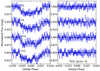 |
Fig. A.1 Left panel: Light curves of HATS-2 obtained from the Sector 10 of NASA’s TESS mission data and used in the analysis of the physical and starspot parameters of the system. They are plotted against the orbital phase and are compared to PRISM/GEMC best-fitting models. The labels indicate the observational ID (see Fig. 3). Right panel: Residuals of the fits represented with the same notation used in the left panel. |
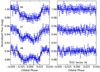 |
Fig. A.2 Left panel: Light curves of HATS-2 obtained from the Sector 36 of NASA’s TESS mission data, and used in the analysis of the physical and starspot parameters of the system. In particular, the image refers only to the transits labelled #6, #7, and #8 (see Fig. 3 and Fig. 5). They are plotted against the orbital phase and are compared to PRISM/GEMC best-fitting models. Right panel: Residuals of the fits represented with the same notation used in the left panel. |
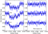 |
Fig. A.3 Left panel: Remaining transit light curves containing spot-crossing events from Sector 36 of NASA’s TESS mission data that were not represented in Fig. A.2. They are plotted against the orbital phase and are compared to new PRISM/GEMC best-fitting models. The labels indicate the observational ID. Right panel: Residuals of the fits represented with the same notation used in the left panel. |
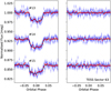 |
Fig. A.4 Left panel: The light curves of HATS-2 obtained from Sector 63 of NASA’s TESS mission data, and used in the analysis of the physical and starspot parameters of the system. In blue are represented the unbinned data, while in red the 10 min cadence binned data. In particular, the image refers only to the transits labelled #13, #14, and #15 (see Fig. 3). They are plotted against the orbital phase and are compared to PRISM/GEMC best-fitting models. Right panel: Residuals of the fits represented with the same notation used in the left panel. |
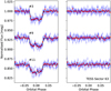 |
Fig. A.5 Left panel: Remaining transit light curves containing spot-crossing events from Sector 63 of NASA’s TESS mission data that were not represented in Fig. A.4. In blue are represented the unbinned data, while in red the 10 min cadence binned data. They are plotted against the orbital phase and are compared to new PRISM/GEMC best-fitting models. The labels indicate the observational ID. Right panel: Residuals of the fits represented with the same notation used in the left panel. |
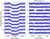 |
Fig. A.6 Left panel: Light curves of eight transits of HATS-2b observed with NASA’s TESS space telescope in Sector 10 of its primary mission. The labels indicate the observation ID (see Fig. 3). They are plotted against the orbital phase and are compared to the best-fitting JKTEBOP models. Right panel: Residuals of each fit. |
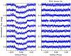 |
Fig. A.7 Left panel: Light curves of eight transits of HATS-2b observed with NASA’s TESS space telescope in Sector 36 of its primary mission. The labels indicate the observation ID (see Fig. 3). They are plotted against the orbital phase and are compared to the best-fitting JKTEBOP models. Right panel: Residuals of each fit. |
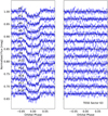 |
Fig. A.8 Left panel: Light curves of 12 transits of HATS-2b observed with NASA’s TESS space telescope in Sector 63 of its primary mission. The labels indicate the observation ID (see Fig. 3). They are plotted against the orbital phase and are compared to the best-fitting PRISM+GEMC models. Right panel: Residuals of each fit. |
Appendix B Mathematical derivation of Section 4.3 equations
Using spherical trigonometry, the relation that connects the longitude ϕ and latitude θ to Cartesian coordinates for a point on a sphere is:
![$\[\left\{\begin{array}{l}x=R_{\star} \cos \theta \cos \phi \\y=R_{\star} \cos \theta \sin \phi \\z=R_{\star} \sin \theta\end{array} \quad.\right.\]$](/articles/aa/full_html/2024/05/aa47872-23/aa47872-23-eq31.png) (B.1)
(B.1)
Referring to Fig. B.1, the sky-projected obliquity is given by:
![$\[\lambda=\arctan \frac{\mathrm{BC}}{\mathrm{AC}}=\arctan \frac{z_2-z_1}{y_2-y_1}.\]$](/articles/aa/full_html/2024/05/aa47872-23/aa47872-23-eq32.png) (B.2)
(B.2)
To obtain the rotational period a proportion must be considered: Prot: 2πR* = Δt: AB. Using Pythagorean theorem is possible to derive the Equation in Section 4.3.
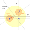 |
Fig. B.1 Geometry of the problem. The rotation axis differs from the normal to the sky-projected plane, so two consecutive spots are observed at different latitudes and longitudes. |
Appendix C GLS fits of TESS photometry
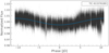 |
Fig. C.1 TESS total light curve (Sectors 10, 36, and 63) in phase with its combined GLS peak of 21.4 days (FAP<0.1% evaluated with the bootstrap method), from the simple aperture photometry (SAP) which was not corrected from long-term trends. The fit of the phased light curve is represented by a blue curve, while the transits of HATS-2 b have been removed. |
Appendix D PRISM/GEMC and JKTEBOP fits of ExoClock data
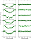 |
Fig. D.1 Left: Light curves of the transits of HATS-2b observed by the astronomers involved in the ExoClock collaboration. They are plotted against the orbital phase and are compared to the best-fitting JKTEBOP and PRISM+GEMC models. The labels indicate in order: observation date, observatory, and observer. DSC stands for Deep Sky Chile, while SSO stands for Sliding Spring Observatory. Right: Residuals of each fit. |
Parameters of the PRISM/GEMC and JKTEBOP best fits of the HATS-2 light curves from the ExoClock database.
Appendix E Extra Table
Parameters of the PRISM/GEMC and JKTEBOP best fits for the HATS-2 light curves used in this work.
References
- Agol, E., Steffen, J., Sari, R., & Clarkson, W. 2005, MNRAS, 359, 567 [Google Scholar]
- Ahrer, E.-M., Stevenson, K. B., Mansfield, M., et al. 2023, Nature, 614, 653 [NASA ADS] [CrossRef] [Google Scholar]
- Ahuir, J., Mathis, S., & Amard, L. 2021, A&A, 651, A3 [NASA ADS] [CrossRef] [EDP Sciences] [Google Scholar]
- Alderson, L., Wakeford, H. R., Alam, M. K., et al. 2023, Nature, 614, 664 [NASA ADS] [CrossRef] [Google Scholar]
- Barros, S. C. C., Akinsanmi, B., Boué, G., et al. 2022, A&A, 657, A52 [NASA ADS] [CrossRef] [EDP Sciences] [Google Scholar]
- Biazzo, K., Bozza, V., Mancini, L., & Sozzetti, A. 2022, in Astrophysics and Space Science Library, 466, Demographics of Exoplanetary Systems, Lecture Notes of the 3rd Advanced School on Exoplanetary Science, 143 [NASA ADS] [CrossRef] [Google Scholar]
- Bonomo, A. S., Desidera, S., Benatti, S., et al. 2017, A&A, 602, A107 [NASA ADS] [CrossRef] [EDP Sciences] [Google Scholar]
- Claret, A. 2004, A&A, 424, 919 [NASA ADS] [CrossRef] [EDP Sciences] [Google Scholar]
- Dai, F., & Winn, J. N. 2017, AJ, 153, 205 [NASA ADS] [CrossRef] [Google Scholar]
- Davies, M. B., Adams, F. C., Armitage, P., et al. 2014, in Protostars and Planets VI, eds. H. Beuther, R. S. Klessen, C. P. Dullemond, & T. Henning, 787 [Google Scholar]
- Demarque, P., Woo, J.-H., Kim, Y.-C., & Yi, S. K. 2004, ApJS, 155, 667 [NASA ADS] [CrossRef] [Google Scholar]
- Eastman, J., Siverd, R., & Gaudi, B. S. 2010, PASP, 122, 935 [Google Scholar]
- Edwards, B., Ho, C., Osborne, H., et al. 2021, Astron. Theory Observ. Methods, 2, 25 [NASA ADS] [CrossRef] [Google Scholar]
- Feinstein, A. D., Radica, M., Welbanks, L., et al. 2023, Nature, 614, 670 [NASA ADS] [CrossRef] [Google Scholar]
- Fortney, J. J., Shabram, M., Showman, A. P., et al. 2010, ApJ, 709, 1396 [NASA ADS] [CrossRef] [Google Scholar]
- Gimenez, A., & Garcia-Pelayo, J. M. 1983, Ap&SS, 92, 203 [NASA ADS] [CrossRef] [Google Scholar]
- Girardi, L., Bressan, A., Bertelli, G., & Chiosi, C. 2000, A&AS, 141, 371 [NASA ADS] [CrossRef] [EDP Sciences] [Google Scholar]
- Greiner, J., Bornemann, W., Clemens, C., et al. 2008, PASP, 120, 405 [Google Scholar]
- Hagey, S. R., Edwards, B., & Boley, A. C. 2022, AJ, 164, 220 [NASA ADS] [CrossRef] [Google Scholar]
- Hartman, J. D., Bakos, G. Á., Sato, B., et al. 2011, ApJ, 726, 52 [NASA ADS] [CrossRef] [Google Scholar]
- Hippke, M., David, T. J., Mulders, G. D., & Heller, R. 2019, AJ, 158, 143 [Google Scholar]
- Johnson, J. A., Winn, J. N., Cabrera, N. E., & Carter, J. A. 2009, ApJ, 692, L100 [NASA ADS] [CrossRef] [Google Scholar]
- Kervella, P., Thévenin, F., Di Folco, E., & Ségransan, D. 2004, A&A, 426, 297 [NASA ADS] [CrossRef] [EDP Sciences] [Google Scholar]
- Kipping, D. M. 2010, MNRAS, 408, 1758 [Google Scholar]
- Kokori, A., Tsiaras, A., Edwards, B., et al. 2022, Exp. Astron., 53, 547 [NASA ADS] [CrossRef] [Google Scholar]
- Kokori, A., Tsiaras, A., Edwards, B., et al. 2023, ApJS, 265, 4 [NASA ADS] [CrossRef] [Google Scholar]
- Kovacs, G., Dékány, I., Karamiqucham, B., et al. 2022, A&A, 664, A47 [NASA ADS] [CrossRef] [EDP Sciences] [Google Scholar]
- Kreidberg, L. 2015, PASP, 127, 1161 [Google Scholar]
- Kurucz, R. L. 1979, ApJS, 40, 1 [NASA ADS] [CrossRef] [Google Scholar]
- Lecavelier Des Etangs, A., Pont, F., Vidal-Madjar, A., & Sing, D. 2008, A&A, 481, L83 [NASA ADS] [CrossRef] [Google Scholar]
- Lightkurve Collaboration, (Cardoso, J. V. d. M., et al.) 2018, Lightkurve: Kepler and TESS time series analysis in Python, Astrophysics Source Code Library, [record ascl:1812.013] [Google Scholar]
- Lin, D. N. C., Bodenheimer, P., & Richardson, D. C. 1996, Nature, 380, 606 [Google Scholar]
- Maciejewski, G., Dimitrov, D., Mancini, L., et al. 2016, Acta Astron., 66, 55 [NASA ADS] [Google Scholar]
- Mancini, L., Ciceri, S., Chen, G., et al. 2013, MNRAS, 436, 2 [Google Scholar]
- Mancini, L., Southworth, J., Ciceri, S., et al. 2014a, A&A, 562, A126 [NASA ADS] [CrossRef] [EDP Sciences] [Google Scholar]
- Mancini, L., Southworth, J., Ciceri, S., et al. 2014b, MNRAS, 443, 2391 [Google Scholar]
- Mancini, L., Esposito, M., Covino, E., et al. 2015, A&A, 579, A136 [NASA ADS] [CrossRef] [EDP Sciences] [Google Scholar]
- Mancini, L., Lillo-Box, J., Southworth, J., et al. 2016, A&A, 590, A112 [NASA ADS] [CrossRef] [EDP Sciences] [Google Scholar]
- Mancini, L., Southworth, J., Raia, G., et al. 2017, MNRAS, 465, 843 [NASA ADS] [CrossRef] [Google Scholar]
- Mancini, L., Esposito, M., Covino, E., et al. 2018, A&A, 613, A41 [NASA ADS] [CrossRef] [EDP Sciences] [Google Scholar]
- Mancini, L., Esposito, M., Covino, E., et al. 2022a, A&A, 664, A162 [NASA ADS] [CrossRef] [EDP Sciences] [Google Scholar]
- Mancini, L., Southworth, J., Naponiello, L., et al. 2022b, MNRAS, 509, 1447 [Google Scholar]
- McIntosh, P. S. 1990, Sol. Phys., 125, 251 [NASA ADS] [CrossRef] [Google Scholar]
- Mohler-Fischer, M., Mancini, L., Hartman, J. D., et al. 2013, A&A, 558, A55 [NASA ADS] [CrossRef] [EDP Sciences] [Google Scholar]
- Newville, M., Stensitzki, T., Allen, D. B., & Ingargiola, A. 2014, https://doi.org/10.5281/zenodo.11813 [Google Scholar]
- Oshagh, M., Santos, N. C., Boisse, I., et al. 2013, A&A, 556, A19 [NASA ADS] [CrossRef] [EDP Sciences] [Google Scholar]
- Oshagh, M., Santos, N. C., Ehrenreich, D., et al. 2014, A&A, 568, A99 [NASA ADS] [CrossRef] [EDP Sciences] [Google Scholar]
- Patra, K. C., Winn, J. N., Holman, M. J., et al. 2017, AJ, 154, 4 [Google Scholar]
- Rabus, M., Alonso, R., Belmonte, J. A., et al. 2009, A&A, 494, 391 [NASA ADS] [CrossRef] [EDP Sciences] [Google Scholar]
- Ragozzine, D., & Wolf, A. S. 2009, ApJ, 698, 1778 [Google Scholar]
- Rasio, F. A., & Ford, E. B. 1996, Science, 274, 954 [Google Scholar]
- Raymond, S. N., & Morbidelli, A. 2022, in Demographics of Exoplanetary Systems, Lecture Notes of the 3rd Advanced School on Exoplanetary Science, eds. K. Biazzo, V. Bozza, L. Mancini, & A. Sozzetti, Astrophysics and Space Science Library, 466, 3 [NASA ADS] [CrossRef] [Google Scholar]
- Ricker, G. R., Winn, J. N., Vanderspek, R., et al. 2014, SPIE Conf. Ser., 9143, 914320 [Google Scholar]
- Rosário, N. M., Barros, S. C. C., Demangeon, O. D. S., & Santos, N. C. 2022, A&A, 668, A114 [NASA ADS] [CrossRef] [EDP Sciences] [Google Scholar]
- Rustamkulov, Z., Sing, D. K., Mukherjee, S., et al. 2023, Nature, 614, 659 [NASA ADS] [CrossRef] [Google Scholar]
- Silva, A. V. R. 2003, ApJ, 585, L147 [Google Scholar]
- Smith, J. C., Stumpe, M. C., Van Cleve, J. E., et al. 2012, PASP, 124, 1000 [Google Scholar]
- Southworth, J. 2008, MNRAS, 386, 1644 [NASA ADS] [CrossRef] [Google Scholar]
- Southworth, J. 2011, MNRAS, 417, 2166 [Google Scholar]
- Southworth, J., Hinse, T. C., Jørgensen, U. G., et al. 2009, MNRAS, 396, 1023 [NASA ADS] [CrossRef] [Google Scholar]
- Southworth, J., Bruni, I., Mancini, L., & Gregorio, J. 2012a, MNRAS, 420, 2580 [CrossRef] [Google Scholar]
- Southworth, J., Hinse, T. C., Dominik, M., et al. 2012b, MNRAS, 426, 1338 [NASA ADS] [CrossRef] [Google Scholar]
- Southworth, J., Mancini, L., Madhusudhan, N., et al. 2017, AJ, 153, 191 [CrossRef] [Google Scholar]
- Southworth, J., Barker, A. J., Hinse, T. C., et al. 2022, MNRAS, 515, 3212 [NASA ADS] [CrossRef] [Google Scholar]
- Stassun, K. G., Collins, K. A., & Gaudi, B. S. 2017, AJ, 153, 136 [Google Scholar]
- Stumpe, M. C., Smith, J. C., Catanzarite, J. H., et al. 2014, PASP, 126, 100 [Google Scholar]
- Sun, X., Bobra, M. G., Hoeksema, J. T., et al. 2015, ApJ, 804, L28 [Google Scholar]
- Ter Braak, C. J. F. 2006, Stat. Comput., 16, 239 [Google Scholar]
- Tregloan-Reed, J., Southworth, J., & Tappert, C. 2013, MNRAS, 428, 3671 [Google Scholar]
- Tregloan-Reed, J., Southworth, J., Burgdorf, M., et al. 2015, MNRAS, 450, 1760 [Google Scholar]
- Turner, J. D., Flagg, L., Ridden-Harper, A., & Jayawardhana, R. 2022, AJ, 163, 281 [NASA ADS] [CrossRef] [Google Scholar]
- VanderPlas, J. T. 2018, ApJS, 236, 16 [Google Scholar]
- Ward, W. R. 1997, ApJ, 482, L211 [NASA ADS] [CrossRef] [Google Scholar]
- Winn, J. N. 2010, in Exoplanets, ed. S. Seager, 55 [Google Scholar]
- Winn, J. N., Holman, M. J., Henry, G. W., et al. 2007, AJ, 133, 1828 [NASA ADS] [CrossRef] [Google Scholar]
- Winn, J. N., Fabrycky, D., Albrecht, S., & Johnson, J. A. 2010, ApJ, 718, L145 [Google Scholar]
- Wong, I., Shporer, A., Vissapragada, S., et al. 2022, AJ, 163, 175 [NASA ADS] [CrossRef] [Google Scholar]
- Wu, Y., & Murray, N. 2003, ApJ, 589, 605 [Google Scholar]
The TEPCat catalogue is available at http://www.astro.keele.ac.uk/jkt/tepcat (Southworth 2011).
The pressure scale height of a planetary atmosphere is defined as H = kBTeq/μmgp, where kB is the Boltzmann constant and μm is the mean molecular weight, for which the value of 2.3 amu is usually adopted for giant planets (Lecavelier Des Etangs et al. 2008).
All Tables
Starspot parameters derived from the PRISM+GEMC fits of the transit light curves.
Median values and 68% confidence intervals of the physical and orbital properties of the HATS-2 system, found using JKTABSDIM.
Best-fit parameters of the ephemeris models for the HATS-2b mid-transit time residuals.
Parameters of the PRISM/GEMC and JKTEBOP best fits of the HATS-2 light curves from the ExoClock database.
Parameters of the PRISM/GEMC and JKTEBOP best fits for the HATS-2 light curves used in this work.
All Figures
|
Fig. 1 Transits from the DK telescope. Left panel: light curves of 11 transits (10 complete and one partial) of HATS-2 b observed with the Danish 1.54 m telescope, shown in chronological order. They are plotted against the orbital phase and are compared to the best-fitting models. Labels indicate the observation date and the filter (Bessell I and R) that was used for each data set. Starspot anomalies are visible in all the light curves. Right-hand panel: the residuals of each fit. |
| In the text | |
|
Fig. 2 Light curves of four (three complete and one partial) transits of HATS-2 b simultaneously observed in four optical bands (Sloan g′, r′, i′, z′) with the GROND multi-band camera at the MPG 2.2 m telescope. They are shown in date order. The light curves in the top panels are from Mohler-Fischer et al. (2013), while those in the bottom panels are from this work. Starspot anomalies are visible in the first three data sets. The light curves are plotted against the orbital phase and are compared to the best-fitting models. The residuals of the fits are shown at the base of each panel. |
| In the text | |
|
Fig. 3 Photometric monitoring of HATS-2 by the TESS space telescope. Top panel: data from Sector 10. Middle panel: data from Sector 36. Bottom panel: data from Sector 63. Fifteen transit events of HATS-2 b were detected by TESS in Sector 10 and 15 in Sector 36, while 18 transit events were detected in Sector 63. |
| In the text | |
|
Fig. 4 Variation in the starspot contrast with wavelength. The vertical bars represent the errors in the measurements and the horizontal bars show the FWHM transmission of the passbands used. In the upper panels, the colour of the data points is in agreement with Fig. 2. In the top left panel, the data taken on 2012 February 28 with the GROND multi-band camera are represented together with the ATLAS9 (Kurucz 1979) stellar atmospherical models computed considering a stellar surface at 5227 K and a starspot at 4200 and 4400 K. In the top right panel, the data taken on 2012 June 1st with the GROND multi-band camera are represented together with the ATLAS9 stellar atmospherical models computed considering a stellar surface at 5227 K and a starspot at 4600, 4850, and 4980 K. In the bottom panels, the points represent the contrast values obtained using the Danish 1.54 m transits (as explained in the plot legend), while the curves are the same ATLAS9 models used in the upper panels. |
| In the text | |
|
Fig. 5 Representation of the stellar disc, starspot position, and transit chord for the two consecutive transit events, #7 (left panel) and #8 (right panel) with starspot crossings, obtained using PRISM/GEMC. The grey scale of each starspot is related to its contrast. The starspot properties refer to the best-fitting models in Fig. A.2 (see Appendix). |
| In the text | |
|
Fig. 6 Sky-projected obliquity as a function of the host stars’ effective temperature for an ensemble of exoplanetary systems. The star is the value of the sky-projected obliquity of the HATS-2 system found in this work, while the dots are the values from the TEPCAT catalogue. |
| In the text | |
|
Fig. 7 Top panel: O–C residuals for HATS-2b in the case (a), superimposed with the best-fitting linear ephemeris model (black line), the best-fitting quadratic ephemeris model (red line) and the best-fitting cosinusoidal ephemeris model (cyan line). The purple points represent the times derived from the Danish 1.54 m telescope observations, the yellow points the times derived from the MPG/ESO 2.2 m telescope data, and the blue points the times derived from TESS data. Bottom panel: same as the top panel but for case (b), i.e. also considering the data from the ExoClock database, which are represented as green points. |
| In the text | |
|
Fig. 8 Stellar tidal quality factor as a function of stellar age for HATS-2 and an ensemble of host stars. These stars were selected considering systems where tidal decay has been observed or is a possible explanation for the observed TTVs (Hagey et al. 2022; Rosário et al. 2022; Wong et al. 2022; Mancini et al. 2022b; Barros et al. 2022). |
| In the text | |
|
Fig. 9 Top panel: variation in the planetary radius, in terms of the planet-to-star radius ratio, with wavelength. The points are from the ground-based transit observations presented in this work (black from the MPG 2.2 m telescope and grey from the Danish 1.54m telescope). The vertical bars represent the errors in the measurements and the horizontal bars show the FWHM transmission of the passbands used. The observational points are compared with three synthetic spectra from Fortney et al. (2010, Red: equilibrium-chemistry; Blue: no TiO, VO opacity; Green: enhanced Rayleigh scattering). The same offset is applied to all four models to provide the best fit to the measurements. The size of 10 atmospheric pressure scale heights (10 × H) is shown on the right of the plot. Bottom panel: transmission curves for the Bessell I and R filters and the total efficiencies of the GROND filters. |
| In the text | |
|
Fig. 10 HATS-2b phase curve obtained by phase-binning the data from Sectors 10, 36 and 63 of NASA’s TESS mission plotted against theoretical curves computed thanks to the batman Python package. |
| In the text | |
|
Fig. A.1 Left panel: Light curves of HATS-2 obtained from the Sector 10 of NASA’s TESS mission data and used in the analysis of the physical and starspot parameters of the system. They are plotted against the orbital phase and are compared to PRISM/GEMC best-fitting models. The labels indicate the observational ID (see Fig. 3). Right panel: Residuals of the fits represented with the same notation used in the left panel. |
| In the text | |
|
Fig. A.2 Left panel: Light curves of HATS-2 obtained from the Sector 36 of NASA’s TESS mission data, and used in the analysis of the physical and starspot parameters of the system. In particular, the image refers only to the transits labelled #6, #7, and #8 (see Fig. 3 and Fig. 5). They are plotted against the orbital phase and are compared to PRISM/GEMC best-fitting models. Right panel: Residuals of the fits represented with the same notation used in the left panel. |
| In the text | |
|
Fig. A.3 Left panel: Remaining transit light curves containing spot-crossing events from Sector 36 of NASA’s TESS mission data that were not represented in Fig. A.2. They are plotted against the orbital phase and are compared to new PRISM/GEMC best-fitting models. The labels indicate the observational ID. Right panel: Residuals of the fits represented with the same notation used in the left panel. |
| In the text | |
|
Fig. A.4 Left panel: The light curves of HATS-2 obtained from Sector 63 of NASA’s TESS mission data, and used in the analysis of the physical and starspot parameters of the system. In blue are represented the unbinned data, while in red the 10 min cadence binned data. In particular, the image refers only to the transits labelled #13, #14, and #15 (see Fig. 3). They are plotted against the orbital phase and are compared to PRISM/GEMC best-fitting models. Right panel: Residuals of the fits represented with the same notation used in the left panel. |
| In the text | |
|
Fig. A.5 Left panel: Remaining transit light curves containing spot-crossing events from Sector 63 of NASA’s TESS mission data that were not represented in Fig. A.4. In blue are represented the unbinned data, while in red the 10 min cadence binned data. They are plotted against the orbital phase and are compared to new PRISM/GEMC best-fitting models. The labels indicate the observational ID. Right panel: Residuals of the fits represented with the same notation used in the left panel. |
| In the text | |
|
Fig. A.6 Left panel: Light curves of eight transits of HATS-2b observed with NASA’s TESS space telescope in Sector 10 of its primary mission. The labels indicate the observation ID (see Fig. 3). They are plotted against the orbital phase and are compared to the best-fitting JKTEBOP models. Right panel: Residuals of each fit. |
| In the text | |
|
Fig. A.7 Left panel: Light curves of eight transits of HATS-2b observed with NASA’s TESS space telescope in Sector 36 of its primary mission. The labels indicate the observation ID (see Fig. 3). They are plotted against the orbital phase and are compared to the best-fitting JKTEBOP models. Right panel: Residuals of each fit. |
| In the text | |
|
Fig. A.8 Left panel: Light curves of 12 transits of HATS-2b observed with NASA’s TESS space telescope in Sector 63 of its primary mission. The labels indicate the observation ID (see Fig. 3). They are plotted against the orbital phase and are compared to the best-fitting PRISM+GEMC models. Right panel: Residuals of each fit. |
| In the text | |
|
Fig. B.1 Geometry of the problem. The rotation axis differs from the normal to the sky-projected plane, so two consecutive spots are observed at different latitudes and longitudes. |
| In the text | |
|
Fig. C.1 TESS total light curve (Sectors 10, 36, and 63) in phase with its combined GLS peak of 21.4 days (FAP<0.1% evaluated with the bootstrap method), from the simple aperture photometry (SAP) which was not corrected from long-term trends. The fit of the phased light curve is represented by a blue curve, while the transits of HATS-2 b have been removed. |
| In the text | |
|
Fig. D.1 Left: Light curves of the transits of HATS-2b observed by the astronomers involved in the ExoClock collaboration. They are plotted against the orbital phase and are compared to the best-fitting JKTEBOP and PRISM+GEMC models. The labels indicate in order: observation date, observatory, and observer. DSC stands for Deep Sky Chile, while SSO stands for Sliding Spring Observatory. Right: Residuals of each fit. |
| In the text | |
Current usage metrics show cumulative count of Article Views (full-text article views including HTML views, PDF and ePub downloads, according to the available data) and Abstracts Views on Vision4Press platform.
Data correspond to usage on the plateform after 2015. The current usage metrics is available 48-96 hours after online publication and is updated daily on week days.
Initial download of the metrics may take a while.