| Issue |
A&A
Volume 684, April 2024
|
|
|---|---|---|
| Article Number | A23 | |
| Number of page(s) | 21 | |
| Section | Numerical methods and codes | |
| DOI | https://doi.org/10.1051/0004-6361/202347255 | |
| Published online | 01 April 2024 | |
Fitting pseudo-Sérsic (Spergel) light profiles to galaxies in interferometric data: The excellence of the uυ-plane
1
Purple Mountain Observatory, Chinese Academy of Sciences,
10 Yuanhua Road,
Nanjing
210023, PR China
e-mail: This email address is being protected from spambots. You need JavaScript enabled to view it.
2
Université Paris-Saclay, Université Paris Cité, CEA, CNRS, AIM,
91191
Gif-sur-Yvette, France
3
Institut de Radioastronomie Millimétrique,
300 Rue de la Piscine,
38406
Saint-Martin-d’Hères, France
4
National Radio Astronomy Observatory,
800 Bradbury Dr., SE Ste 235,
Albuquerque, NM
87106, USA
5
LERMA, Observatoire de Paris, PSL Research University, CNRS, Sorbonne Universités,
75014
Paris, France
6
Kavli Institute for the Physics and Mathematics of the Universe, The University of Tokyo,
Kashiwa,
277-8583, Japan
7
Kavli Institute for Astronomy and Astrophysics, Peking University,
Beijing
100871, PR China
8
Center for Data-Driven Discovery, Kavli IPMU (WPI), UTIAS, The University of Tokyo,
Kashiwa, Chiba
277-8583, Japan
9
Department of Astronomy, School of Science, The University of Tokyo,
7-3-1 Hongo, Bunkyo,
Tokyo
113-0033, Japan
10
School of Physics and Astronomy, University of Southampton,
Highfield
SO17 1BJ, UK
11
Center for Extragalactic Astronomy, Department of Physics, Durham University,
South Road,
Durham
DH1 3LE, UK
12
National Astronomical Research Institute of Thailand,
Don Kaeo, Mae Rim, Chiang Mai
50180, Thailand
13
Department of Physics, Faculty of Science, Chulalongkorn University,
254 Phayathai Road,
Pathumwan, Bangkok
10330, Thailand
14
European Southern Observatory,
Karl-Schwarzschild-Str. 2,
D-85748
Garching bei Munchen, Germany
15
Cosmic Dawn Center (DAWN),
Denmark
Received:
22
June
2023
Accepted:
7
December
2023
Abstract
Modern (sub)millimeter interferometers, such as ALMA and NOEMA, offer high angular resolution and unprecedented sensitivity. This provides the possibility to characterize the morphology of the gas and dust in distant galaxies. To assess the capabilities of the current software in recovering morphologies and surface brightness profiles in interferometric observations, we tested the performance of the Spergel model for fitting in the uυ-plane, which has been recently implemented in the IRAM software GILDAS (uv_fit). Spergel profiles provide an alternative to the Sérsic profile, with the advantage of having an analytical Fourier transform, making them ideal for modeling visibilities in the uυ-plane. We provide an approximate conversion between the Spergel index and the Sérsic index, which depends on the ratio of the galaxy size to the angular resolution of the data. We show through extensive simulations that Spergel modeling in the uυ-plane is a more reliable method for parameter estimation than modeling in the image plane, as it returns parameters that are less affected by systematic biases and results in a higher effective signal-to-noise ratio. The better performance in the uυ-plane is likely driven by the difficulty of accounting for a correlated signal in interferometric images. Even in the uυ-plane, the integrated source flux needs to be at least 50 times larger than the noise per beam to enable a reasonably good measurement of a Spergel index. We characterized the performance of Spergel model fitting in detail by showing that parameter biases are generally low (<10%) and that uncertainties returned by uv_fit are reliable within a factor of two. Finally, we showcase the power of Spergel fitting by reexamining two claims of extended halos around galaxies from the literature, showing that galaxies and halos can be successfully fitted simultaneously with a single Spergel model.
Key words: methods: data analysis / techniques: interferometric / galaxies: high-redshift / submillimeter: galaxies
Anniversary Fellow.
© The Authors 2024
 Open Access article, published by EDP Sciences, under the terms of the Creative Commons Attribution License (https://creativecommons.org/licenses/by/4.0), which permits unrestricted use, distribution, and reproduction in any medium, provided the original work is properly cited.
This article is published in open access under the Subscribe to Open model. This email address is being protected from spambots. You need JavaScript enabled to view it. to support open access publication.
1 Introduction
Galaxy morphologies are closely linked to their formation and evolution (e.g., Conselice 2014). One of the most effective ways to understand the structures of galaxies and how they evolved over time is by measuring the distribution of light within them, specifically in relation to their radial distance from the center (e.g., Tacchella et al. 2015). To describe the morphological types of galaxies, two commonly used measurements are the halflight radius and the central concentration of light profiles (e.g., the Sérsic index). These measurements provide insights into the shapes and sizes of galaxies and help classify them into different morphological categories.
Over the past decade, optical and near-infrared (IR) observations have allowed for the exploration of the structural properties of the stellar components in high-redshift star-forming galaxies (e.g., Wuyts et al. 2011; van der Wel et al. 2014; Shibuya et al. 2015; Tacchella et al. 2018; Cutler et al. 2022; Chen et al. 2022; Kartaltepe et al. 2023). However, obtaining measurements of purely star-forming components based on ultraviolet and optical star-formation rate tracers are much more difficult, due to the effects of dust attenuation. At high redshifts, galaxy morphology can manifest in various ways, ranging from radial gradients (Nelson et al. 2016) to very complex asymmetrical distributions (Le Bail et al. 2023). In massive (M* > 1010 M⊙) galaxies, most of the rest-frame UV and optical emission is re-emitted in the far-IR and submillimeter windows (e.g., Pannella et al. 2015; Wang et al. 2019; Fudamoto et al. 2021; Smail et al. 2021; Xiao et al. 2023; Gómez-Guijarro et al. 2023), which provide an excellent alternative to obtain unbiased measurements of the morphology of star formation inside galaxies.
Recent developments in (sub)millimeter interferometers, such as ALMA and NOEMA, have made it possible to study the distribution of dust and molecular gas in high-redshift galaxies with high sensitivity (e.g., Barro et al. 2016; Hodge et al. 2016, 2019; Tadaki et al. 2017; Elbaz et al. 2018; Fujimoto et al. 2018; Gullberg et al. 2019; Jiménez-Andrade et al. 2019; Puglisi et al. 2019, 2021; Gómez-Guijarro et al. 2022; Stuber et al. 2023). This provides new observational constraints to the distribution of gas and dust-obscured star formation in galaxies. The ALMA instrument, which has the widest array of configurations, can potentially deliver very high spatial resolution, on the order of a few tens of milliarcseconds (depending on frequency), which is unparalleled, even by HST and JWST standards. The ALMA instrument has already revealed the complex structure of star formation on sub-kiloparsec scales in dusty star-forming galaxies (e.g., Iono et al. 2016; Gullberg et al. 2018; Hodge et al. 2019; Rujopakarn et al. 2019). Comparing star-formation profiles with stellar mass profiles and morphology (more in general) is crucial to understanding the structural evolution of galaxies as a result of star formation (e.g., Cibinel et al. 2015). To extract the full amount of information contained in the data, it is also essential to have the appropriate technical tools. For example, ALMA and NOEMA interferometers gather data in the form of visibilities between antennas in the uυ-plane, unlike the optical data, which are images directly from CCDs or other electronic detectors.
So far, modeling galaxy morphology profiles in the submillimeter, based on interferometric data, has typically involved reconstructing images from the visibilities followed by featuring Sérsic (or other kinds of) profile fitting. This approach has been necessary due to the lack of an effective way to fit generic Sér-sic profiles in the uυ-plane, as supported by common software packages dedicated to the calibration and analysis of radio-interferometric data (e.g., CASA, AIPS, MIRIAD, GILDAS; a summary of profiles provided by each software package in the visibility modeling has been given by Martí-Vidal et al. 2014).
Visibilities are the immediate output of interferometric observations that sample the Fourier transform of the sky brightness distribution and consist of amplitudes and phases (depending on angles between antenna pairs as projected on the sky). The amplitudes and phases can be represented as imaginary numbers in the uυ-plane, with their uυ elongation depending on antenna separation and frequency. As the Earth rotates, each pair of antennas in the interferometric array traces out an elliptical track in the uυ-plane. The Fourier transform of the measured visibilities produces a dirty image. The point-spread function (PSF) of the resulting image, known as the “dirty beam”, has a complex shape with, even in case of relatively good sampling of the uυ-plane, numerous positive and negative sidelobes extending to large spatial scales.
As each data element in the uυ-plane (visibility) affects the data at all spatial scales via the Fourier transform, the signal as well as the noise in the resulting images are always strongly correlated, especially on scales according to the full width at half maximum (FWHM) of the dirty beam. This correlation can significantly impact the measurements of a source’s structure (e.g., Condon 1997; Martí-Vidal et al. 2014; Pavesi et al. 2018; Tsukui et al. 2023). When analyzing image-based measurements, it has been shown that ignoring signal correlation in interferometric images can lead to a significant underestimation of statistical uncertainties and, consequently, misinterpreted results (Tsukui et al. 2023). However, many recent studies (e.g., Elbaz et al. 2018; Fujimoto et al. 2018; Hodge et al. 2019; Lang et al. 2019; Fudamoto et al. 2022) measured submillimeter morphologies in the image plane using tools such as galfit (Peng et al. 2002, 2010). These tools are optimized for optical and near-IR observations and, as such, do not account for the complex noise correlation typical of interferometric observations.
Interferometric images are often cleaned during deconvolution, a process which replaces the dirty beam with well-defined PSFs. However, these routines are based on strong assumptions and are not fully objective. Moreover, they do not account for the strong correlation between pixels on the scale of the beam. For example, high-fidelity observations of z ~ 3 star-forming galaxies by Rujopakarn et al. (2019) using ALMA show that the small-scale source structures of galaxies are affected by both the weighting scheme and the cleaning (deconvolution) algorithm in imaging procedures.
In contrast, working directly in the uυ-plane would be preferable because the measured data points therein are independent. For example, it has been suggested that analyzing observations of very compact sources in Fourier space is more reliable than image-based analyses (Martí-Vidal et al. 2012). However, the lack of tools that allow general profile fitting in the uυ-plane represents an obstacle. Typical codes allow for Gaussian fitting in addition to the standard PSF fitting and sometimes exponential profiles (i.e., the particular case of n = 1 for the Sérsic profile).
One possible way to approximate the standard surface brightness profile (i.e., general Sérsic) of galaxies is to use linear superpositions of Gaussians (Hogg & Lang 2013). However, this approach has limitations. For example, it is difficult to precisely measure how the light is concentrated in the center of galaxies, and the comparison to results obtained in optical and near-IR bands becomes prohibitive. This is because general Sérsic profiles are not analytically transformable into Fourier space, making it computationally intensive to fit a Sérsic profile to visibilities that require large numbers of numerical Fourier transforms while fitting the model to the data.
Quite conveniently, the issue with the lack of analytical Fourier transformability of the Sérsic profile has already been addressed in the framework of optical imaging, where it became necessary to account for spatially and temporally varying PSFs, which requires computationally intensive convolutions. Spergel (2010) proposed a solution based on the incomplete Bessel function of the third kind. This function closely approximates Sérsic functions and is commonly known as the Spergel profile (see Sect. 2.2 for a description of the profile). The Spergel profile has also recently been incorporated into the MAPPING procedure of GILDAS1 (Guilloteau & Lucas 2000). This allows for the study of a galaxy’s morphology in interferometric observations with unprecedented detail, enabling comparison to optical studies. The idea of this approach is to model galaxy structures accurately using functions that approximate the Sérsic profile in the uv-plane (i.e., pseudo-Sérsic).
Modeling the galaxy submillimeter structure using a Spergel profile has been discussed for selected examples of high-redshift star-forming galaxies (Kalita et al. 2022; Rujopakarn et al. 2023). However, despite the novelty of the exercise, there are no attempts in the literature to systematically characterize the performances of Spergel modeling of light profiles of galaxies in the uυ-plane. This includes the returned fidelity and accuracy in parameter estimation, required signal-to-noise ratios (S/Ns) for attempting complex modeling, and possible degeneracies between parameters. This is similar to what has been extensively done in the optical images for galfit and other tools during the past decades (e.g., Moriondo et al. 2000; Pignatelli et al. 2006; Häussler et al. 2007; Mancini et al. 2010; Hoyos et al. 2011; Hiemer et al. 2014; Lange et al. 2016; Tortorelli & Mercurio 2023, and many others). Additionally, the conversion of Spergel indices to Sérsic indices, which enables the comparison of sub-millimeter and millimeter measurements of Spergel profiles to those derived from the classic approach of galaxy light profile modeling (i.e., galfit; Peng et al. 2002), was only briefly explored by Spergel (2010).
In this paper, we aim to provide a technical assessment of the use of the Spergel profile. Our investigation focuses on the robustness of profile fitting with Spergel models using simulated data with real noise from actual observations, and we compare this approach with the traditional application of profile fitting on reconstructed interferometric images. We plan to use these results to perform Spergel modeling on a large galaxy sample taken from the ALMA archive in a forthcoming paper (Q. Tan et al., in prep.).
The paper is structured as follows. In Sect. 2, we recall the definition of the radial profile functions used to constrain the light profile of galaxies in the image plane (Sérsic) and uυ-plane (Spergel), respectively. We compare the two profiles and discuss how their parameters can be converted from one to the other for this comparison. Section 3 introduces the method used to generate the simulated data, with a description of the uv_fit algorithm. In Sect. 4, we present the results of a study that tested the robustness of the profile fitting in the uυ-plane against model fits to image data. This includes a comparison of the recovery of the structural parameters and the accuracy of the measurements. Analyses of the absolute accuracy of the uυ-plane modeling, the reliability of parameter uncertainties, and the covariance of fitted parameters are described in Sect. 5. In Sect. 6, we discuss the simulation results and explore possible reasons for the different measurement performances of interferometric data. We also discuss the implication for the study of galaxy morphology using an example based on re-examining previously published ALMA data. The conclusions of the paper are presented in Sect. 7.
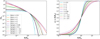 |
Fig. 1 Comparison of surface density profiles (left) and the cumulative distributions (right) for Sérsic (solid lines) and Spergel (dashed lines) functions. The light profile with a Sérsic index of 0.5, 1, 2, 4, and 5 and a Spergel index of 0.85, 0.5, −0.3, −0.6, and −0.7 is shown in different colors. By definition, Re, contains half of the integrated galaxy light. |
2 Sérsic and Spergel radial profile functions
In this section, we first recall the definitions of the Sérsic and Spergel profiles. Then we proceed to a qualitative comparison between the profiles, as their indices vary, emphasizing the role played by the spatial scales actually observed. Finally, we present empirical recipes to convert Spergel indices as well as effective radii and total fluxes to their equivalent Sérsic values. These recipes are used throughout the paper to directly compare Spergel and Sérsic fits under realistic noise conditions from our simulations.
2.1 The Sersic profile
As a generalization of the r1/4 law, the r1/n profile first proposed by Sersic (1968) is one of the most common functions used to describe how the intensity of a galaxy varies with distance from its center. The surface density (or equivalently surface brightness) of the Sérsic profile can be written as
![Mathematical equation: ${\rm{\Sigma }}(R) = {{\rm{\Sigma }}_{\rm{e}}}\exp \,\left[ { - \kappa \,\left( {{{\left( {{R \over {{R_{\rm{e}}}}}} \right)}^{1/n}} - 1} \right)} \right]\,,$](/articles/aa/full_html/2024/04/aa47255-23/aa47255-23-eq1.png) (1)
(1)
where R is the projected distance to the source center, Re is the effective radius containing half of the total luminosity, ∑e is the surface brightness at Re, and n is the Sérsic index that determines the shape of the light profile (see Fig. 1). The parameter κ is a function of the Sérsic index and is such that Γ(2n) = 2γ(2n, κ), where Γ and γ represent the complete and incomplete gamma functions (Ciotti & Bertin 1999), respectively. We use the terms “half-light radius” and “effective radius” interchangeably to refer to the radius within which half of a galaxy’s luminosity is contained.
The Sérsic index, n, determines the degree of curvature of the profile, with n = 0.5 giving a Gaussian profile, n = 1 giving an exponential disk profile, and n = 4 generally being associated with galaxy bulges. As the index n increases, the core steepens more rapidly for R < Re, and the intensity of the outer wing at R > Re becomes significantly extended.
However, as mentioned in the introduction, the general Sér-sic profile is not analytically transformable in Fourier space for most values of the parameter n, as the parameter κ cannot be solved in a closed form. Various techniques have been developed to address this issue when calculations of the Fourier transform are needed, including numerical integration methods, approximations, and asymptotic expressions (e.g., Ciotti & Bertin 1999; Mazure & Capelato 2002; Baes & Gentile 2011). The inability to solve the Sérsic profile analytically in Fourier space creates challenges in certain scenarios. For example, when performing convolutions, such as corrections for seeing, or when directly working in Fourier space, as with interferometric data.
2.2 The Spergel profile
Spergel (2010) introduced an alternative to the Sérsic model for galactic luminosity profiles with functional form
 (2)
(2)
where  , Γ is the gamma function, Kv is a modified spherical Bessel function of the third kind, cv is a constant, Re is the half-light radius, and v is known as the Spergel index that controls the relative peakiness of the core and the relative prominence of the wings (similar to Sérsic n), with a theoretical limit of v > −1.
This family of functions has been found to provide a good fit for galaxy light profiles and resembles the Sérsic function over a range of indices. The Spergel profile at v = 0.5 is identical to an exponential profile, which is equivalent to a Sérsic profile with n = 1. However, the two functions do not exactly coincide for different Spergel v (see Fig. 1). The Spergel profile has a significant advantage over the Sérsic profile because it is analytic in both real space and Fourier space (Spergel 2010), which means that it can be described mathematically using equations, making it easier to work with and analyze in the uυ-plane.
2.3 Qualitatively relating the Sérsic and Spergel profiles
In the left panel of Fig. 1, a comparison is shown between the Sérsic and Spergel profiles. This comparison covers a range of n and v indices. All the profiles have been normalized at Re. Within a certain range of v, the Spergel profiles resemble Sérsic profiles in shape such that a relation can be conceived between v and n. For example, the Spergel profile at v = −0.6 and in the radial range near the effective radius exhibits similarities with a de Vaucouleurs n = 4 profile (see also Spergel 2010). However, when elongating far from the normalization point, these profiles start to differ at both the innermost (i.e., R < 0.1 Re) and outermost (i.e., R > 5 Re) regions, indicating that converting one index to the other depends on the observed scales. This is generally the case for all Sérsic models with n > 1, corresponding to their first-order matching Spergel profiles with −1 < v < 0.5. That is, the Spergel profiles display steeper inner profiles and drop faster at large radii. This is discussed further later in this section.
We also observed from Fig. 1 that Spergel models are not meant to reproduce Sérsic models with a flatter shape than n = 1 (i.e., n < 1). For example, even when choosing v = 0.85, the Spergel model only slightly flattens compared to the v = 0.5 (n = 1 ) case, and it remains far from resembling a Gaussian model n = 0.5. Given that fitting Gaussian models in the uυ-plane is a straightforward approach, we suggest using this method instead of attempting Spergel fits with high values of v > 1.
In the right panel of Fig. 1, we show cumulative distributions for the Sérsic and Spergel profiles. When truncated at 10 Re, an exponential profile (Sérsic n = 1 and Spergel v = 0.5) retains almost all of its flux (~100%). In contrast, a Sérsic profile with n = 4 retains 96.1% of its flux, while 99.7% of the flux is contained within this radius for a Spergel profile with v = −0.6. At the small radius, within the inner 0.05 Re, an exponential profile contains 0.3% of the flux, while n = 4 contains 3.2% of the flux. For a Spergel profile with v = −0.6, 5.4% of the flux is contained within this radius. As the index n increases (or decreases for v), the differences between the fluxes contained within the radius of the small and large ends increase somewhat while also remaining contained overall. A comparison of the Sérsic profile with the Spergel profile using mathematical simulations is presented in Fig. A.1.
2.4 Converting the Spergel index into the equivalent Sérsic index
To empirically derive the conversion (spatial-scale dependent) between the Spergel v and the Sérsic n, we created noise-free2 images of two-dimensional Spergel models (described in the next section). We then used galfit to measure the corresponding Sérsic index. In Fig. 2, the cross symbols represent the galfit measurements, which we refer to as the intrinsic best value and label as ngalfit, compared to the input v for different source sizes of Re/θb ranging from 0.1 to 2.0. Here θb is defined as the synthesized circularized beam size given by  , where a and b represent the FWHMs of the major and minor axes of the synthesized beam, respectively.
As a zero-order check of the procedure, Fig. 2 shows that for a Spergel profile with v = 0.5, sources with different sizes all return a Sérsic index of n = 1 in galfit, as expected. This result is accurate within 3%, which represents the inherent maximal precision of this empirical calibration. We find that v = −0.6 corresponds to n = 4 for Re/θb, ~ 0.9–1.0, which is close to when the FWHM scale of the galaxy and of the beam are identical, as expected (Spergel 2010). However, when Re/θb, < 0.5, an input v = −0.6 converts to n ~ 2–3, while models with v = −0.6 and Re/θb, > 1 correspond to a steeper n > 4. The dependence of the conversion on Re/θb, systematically decreases with increasing Spergel indices and nearly vanishes for v > 0 (Fig. 2).
We found that the whole set of measurements can be well described by the form
 (3)
(3)
for sources with Re/θb, ranging from 0.1 to 2.0, respectively. The solid lines in Fig. 2 represent the best-fit relation with coefficients p1 = 0.0249, p2 = −7.72, p3 = 0.191, p4 = −0.721, and p5 = 1.32. The residuals of the fit indicate that the uncertainties of Sérsic n are largely within 10% for model sources with Re/θb of 0.1–2.0 at v > −0.7 (see Fig. 2). We analytically confirmed this trend when comparing the Spergel index with the Sérsic index through a mathematical matching between the Sérsic and Spergel functions (see Fig. A.2).
This analysis demonstrates that converting a Spergel index to a Sérsic index depends on the ratio between the angular size of the galaxy and that of the beam of the observations being examined. We mapped this relationship over a reasonably large range of this ratio (i.e., Re/θb, of 0.1–2.0). Anticipating the results from a forthcoming paper that focuses on analyzing the morphologies of an ALMA archival sample of about 100 distant star-forming galaxies in the submillimeter bands (Q. Tan et al., in prep.), we found that around 82% (93%) of the sources fall within the range of Re/θb = 0.1–1.0 (0.1–2.0), while approximately 88% (99%) of the sources exhibit best-fitting v > −0.7 (v < 1). The median Re/θb is 0.32, and the semi-interquartile range is 0.2–0.6. This suggests that the calibration presented in Fig. 2 is representative of general observations of distant galaxies with ALMA and NOEMA.
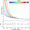 |
Fig. 2 Comparison of Sérsic and Spergel indices. The data (crosses) in the top panel represent the galfit Sérsic indices measured for sources created with the input Spergel model for a range of v values from −0.7 to 0.5 and for different source effective radii (expressed in terms of the FWHM of the synthesized beam, Re/θb) ranging from 0.1 to 2.0. The solid curves in the top panel denote the best-fit empirical relation between Spergel v and galfit Sérsic n, depending on Re/θb, as expressed by Eq. (3). The lower panel displays normalized residuals to the proposed relation. |
2.5 Converting half-light radii and total fluxes from Spergel to Sérsic
The differences in the profiles also imply that for sizes (half-light radii) and total fluxes, a conversion might be required when comparing results based on Spergel to those from Sérsic. Based on our simulations, we found that both the size and flux density estimated by galfit using a Sérsic profile tend to be larger than when using Spergel, as the Sérsic index becomes larger. However, axis ratios and position angles (PAs) remained unaffected. Figure 3 shows the ratios of Re and flux densities measured from fitting Sérsic models to simulated galaxies created as Spergel models as a function of the Spergel index. Both the ratio of Re and flux density exhibit a similar increasing trend as the profile becomes steeper. The ratio becomes larger for better resolved sources (i.e., larger Re/θb). For example, in the case of a large-sized (Re/θb = 1) galaxy with a de Vacouleurs-like profile of v = −0.6, the Re estimated by the Sérsic model can be larger by about 30–40%, while the excess flux density is around 15–20%. By comparison, the relative increase in Re and flux density are less significant for sources with flatter profiles or smaller sizes compared to the beam.
To correct for these systematical biases and thus enable a comparison of measurements using Spergel and Sérsic profiles, we fit the distribution of the ratio of half-light radius and total flux measured from Sérsic to the Spergel-based input values. To distinguish the fitted parameters between those obtained from Spergel versus Sérsic profile modeling, we labelled Re and Ssp as the half-light radius and total flux measured from Spergel profile fitting, respectively. For Sérsic-based measurements, we use instead Re,se and Sse. We found that both ratios of Re,se /Re and SSe/Ssp can be accurately described by a similar form
 (4)
(4)
for sources with Re/θb ranging from 0.1 to 2.0. For the size ratio of Re,se/Re, the best-fit gives the coefficients p1 = 0.00138, p2 = −8.96, p3 = 0.260, p4 = −0.0260, and p5 = 0.996, while for the flux ratio of SSe/Ssp, the best-fit coefficients are p1 = 0.00217, p2 = −7.43, p3 = 0.149, p4 = 0.00942, and p5 = 1.00 (see the solid lines in Fig. 3). Analytical calculations, matching the Spergel profile with Sérsic profiles numerically (see Appendix A) fully confirmed the trends encoded in Eq. (4) above and in Fig. 3.
We caution that while we believe that our methodology captures the bulk of the systematic effects in the conversion as encoded in the Re/θb ratio, some further systematics might be expected depending on higher order terms describing the actual shape of the beam. We derived best-fitting parameters for Eqs. (3) and (4), averaging over three different ALMA array configurations. By comparing the average results to results from a single ALMA array’s configurations, we estimated that further systematic uncertainties are small. The details of the three ALMA array configurations are summarized in Table B.1.
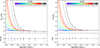 |
Fig. 3 Similar to Fig. 2 but showing the ratio of effective radii (left) and total fluxes (right) obtained from fitting Sérsic models to simulated galaxies created using Spergel profiles (crosses). The data are plotted as a function of their Spergel index. The solid curves denote the best-fit empirical relations as expressed by Eq. (4). The bottom panels show the normalized residuals to the best fit, which are largely within 10%. |
3 Technical aspects: simulating galaxies under realistic noise conditions and measuring their properties
3.1 Realistic noise map
Each simulated galaxy was created by inserting a model source signal into an empty dataset with realistic noise. The noise was obtained from real data using ALMA Band 7 observed visibilities from galaxies in a recent survey (e.g., Puglisi et al. 2019, 2021; Valentino et al. 2020).
To analyze the data, the calibrated ALMA visibilities for several targets were exported from CASA using exportuvfits. The exported data was then converted to uυ-tables using the GILDAS fits_to_uvt task. The four spectral windows were combined using the uv_continuum and uv_merge tasks. Prior to introducing the model source into the uυ-plane, any detected sources were subtracted from the visibility data using the best-fitting Spergel model to the visibilities. This produced a residual dataset, which, upon inspection, did not reveal any further source.
Figure 4 (left) shows the map of the residual uυ data for a case in our simulations. The primary beam field of view (FOV) is 18″, and the FWHM of the synthesized beam using natural weighting is θb = 1.0″. The right panel of Fig. 4 shows the pixel distribution, which can be fitted well with a Gaussian profile. This indicates that the data is mostly noise without any other significant features. The noise level measured from the Gaussian fit is 40 µJy beam−1. We refer to the rms noise derived in this way as σb in the following sections. This is an objective characterization of the noise in the data independent of source properties.
We emphasize that each empty galaxy map can be used for a large number of independent simulations. This can be achieved by placing a simulated signal at random positions within the primary beam. Considering that half-synthesized-beam offsets produce an independent noise realization, the number of such independent realizations are on order of 1000 for each empty ALMA Band 7 dataset.
3.2 Source models
The model sources were created using GILDAS through the MAPPING task uv_fit. We generated elliptical Spergel model sources by fixing the seven free parameters centroid position, flux density, effective radius Re, minor-to-major axis ratio, PA, and Spergel index v3. The flux density varies over a range with a step size of a factor of two. This range corresponds to a total flux density that is normalized by the noise, varying from 25 to 400, which is represented by the ratio of integrated flux density to the pixel rms noise (Stot/σb). We defined the S/N as the ratio of the integrated flux density to the noise per beam Stot/σb. The advantage of this choice is in its model independence and reliance on very basic properties of the source and of the noise. We note that for extended sources, the S/N defined in this way is obviously higher than the S/N eventually recovered for the integrated flux density coming from a full Spergel and Sérsic profile.
The simulation process involved setting the size of the sources in units of θb, that is, Re/θb = 0.1, 0.2, 0.4, and 0.7, in order to represent sources of very compact, small, intermediate, and large sizes (relative to the beam). For each set of Monte Carlo (MC) sources that shared a fixed effective radius and axis ratio q (≡ b/a), the Spergel model sources varied in both their flux density (thus S/N) and Spergel index, with values of v = 0.5, −0.3, −0.5, −0.6, and −0.7. The PA remained constant. To mimic real observations, we added the model sources to the realistic noise data that was derived from the observed visibilities in order to produce a simulated dataset (see Fig. 4 for an example).
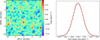 |
Fig. 4 Example of an empty dataset used for our simulations. Left: noise map. The source emission (which was close to the phase center) was subtracted from the visibility data. The dashed white circle represents the primary beam (i.e., the FOV) of the dataset. Right: histogram of pixel values within the primary beam. The red line represents the best-fitting Gaussian model. The fit suggests that the noise data is at least approximately Gaussian. |
3.3 Visibility model fitting with Spergel profile
Fitting the elliptical Spergel models to the simulated dataset was performed using the task uv_f it. All the seven fitted parameters were allowed to vary. As typically done within MAPPING’s uv_fit in GILDAS, we generated a range of initial guesses for each fitted parameter, which were built into an N-dimensional list of combinations of these guesses. This approach helped explore a wider range of possible solutions and thus identify the best-fit model and return a well-sampled range for uncertainties. We tested the fit by setting the starting range parameters of initial guesses within a factor of two centered on the input mock values and the number of start parameters (e.g., three guesses for each parameter). We found that for simulated sources (where model parameters are known a priori), the results using a single initial guess identical to the real parameters were not significantly different from when the code is run using multiple initial guesses for each parameter. However, using uv_f it with a large range of initial guesses is critical for real observations, where the source’s properties are not known beforehand.
3.4 Image model fitting with Sérsic profile
Each uυ-plane simulation was imaged and then fitted with a single-component Sérsic profile using galfit (Peng et al. 2002). The galfit run was performed on the dirty maps, which were created with Fourier transforming visibilities without cleaning. The (full) dirty beam was used as the galfit PSF. The known parameters of the mock sources were used as initial guesses for galfit. All parameters were left free without constraints in the fitting. The initial guess of the Sérsic n was calculated by converting the input v using Eq. (3). The Sérsic fits also provided measurements of seven free parameters: central position, total magnitude, effective radius, Sérsic index, axis ratio, and PA. In some cases, galfit may have failed to provide accurate measurements. To ensure the validity of our comparisons, we removed measurements in both the image plane and uυ-plane for sources with output parameters marked as problematic in galfit. We note that these procedures are extremely favorably biased toward positively amplifying the performances of galfit.
Figure 5 illustrates a typical case of a simulated source generated with a Spergel profile and with a Stot/σb ratio of 50. Additionally, it shows the best-fit models derived from uv_f it and galfit, respectively. Both methods provided good constraints to the simulated source at this S/N, as no significant component is visible in the residual map.
3.5 Details of the UV_FIT implementation in GILDAS
The uv_fit command uses the SLATEC/DNLS1E implementation of the Levenberg-Marquardt algorithm (see Press et al. 1992, for an intuitive presentation) to minimize the reduced χ2 of this non-linear least-square problem. This algorithm only requires the delivery of a routine that computes the complex function and its partial derivatives with respect to the different fitted parameters. Appendix C presents the equations for the elliptical Spergel profile and its partial derivatives. Once the minimum of the least-square problem was found, the routine SLATEC/DCOV was called to compute the covariance matrix at this minimum. The diagonal elements of this covariance matrix are the ± 1σ uncertainties on each fitted parameter.
In estimation theory, the Fisher matrix, IF, quantifies the amount of information in the least-square problem. When the noise on the measurements (the visibilities) is well modeled by an uncorrelated, centered white Gaussian random variable of standard deviation σ, the computation of the Fisher matrix reduces to (Stoica & Moses 2005)
![Mathematical equation: $\forall (i,j)\quad {\left[ {{{\bf{I}}_F}} \right]_{ij}} = \mathop \sum \limits_{k = 1}^{{n_{{\rm{visi}}}}} {1 \over {\sigma _k^2}}{{\partial {V_k}} \over {\partial {\varphi _i}}}{{\partial {V_k}} \over {\partial {\varphi _j}}},$](/articles/aa/full_html/2024/04/aa47255-23/aa47255-23-eq7.png) (5)
(5)
where [IF]ij stands for the term (i,j) of the Fisher matrix, σk and Vk are the noise and the fitted visibility function for visibility k, and (φi) is the vector of fitted parameters. In our case, (φi) = (x0,y0,L0,Rmaj,Rmin, ϕ, v), that is, the central position of the Spergel profile as an offset with respect to the phase center, its luminosity, its major and minor half-light radius, its position angle, and its index. The Cramer-Rao bound (CRB) for each fitted parameter, Ɓ(φi), is defined as the; ith diagonal element of the inverse of the Fisher matrix
![Mathematical equation: $B\left( {{\varphi _i}} \right) = {\left[ {{\bf{I}}_F^{ - 1}} \right]_{ii}}.$](/articles/aa/full_html/2024/04/aa47255-23/aa47255-23-eq8.png) (6)
(6)
The CRB is the reference precision of the least-square problem. Indeed, the variance of any unbiased estimator of the parameter i will always be larger than the associated CRB (Garthwaite et al. 1995), or
 (7)
(7)
In other words, an efficient fitting algorithm will deliver variances for the estimated parameters that reach the associated CRB values. In practice, sufficiently large signal-to-noise ratios are required to ensure that the χ2 minimization converges toward the actual solution. Additional explanations and an example of the application to the fit of CO(1–0) profiles in the local inter-stellar medium can be found in Roueff et al. (2021).
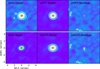 |
Fig. 5 Example of a simulated source generated with a Spergel profile of Stot/σb = 50, Re/θb = 0.4, axis ratio of q = 0.75, PA = 30°, and Spergel index of v = −0.6. From left to right: the dirty image (top-left), dirty beam (PSF used for convolution in galfit; bottom-left), best-fit source models convolved with the dirty beam (middle), and residuals after subtracting the model source (right). The model source and the model-subtracted residual shown in the top and bottom rows were derived from the uv_fit and galfit fits, respectively. Each image cutout is 9″ × 9″. The contours start from 2σ and increase in steps of 4σ. White crosses mark the best-fit source position obtained from uv_fit. |
4 Analysis: comparison of uυ-plane and image-plane performances
In this section, we compare the parameter estimates obtained by fitting the Spergel profile in the uυ-plane and the Sérsic profile in the image plane to the same data and thus comparatively assess their performances for the recovery of all the key parameters. Additionally, we investigate the reliability of the uncertainties returned by the fitting codes. For all parameters, the systematic terms that arise due to the intrinsic differences in the profiles (Sect. 2, see Eqs. (3) and (4)) are always included in the comparison.
4.1 Comparison of structural parameter measurements
In Fig. 6, we present the results of our simulations using only two models of galaxies as typical examples for clarity. The input mock source was chosen with Re/θb of 0.4 (0.2), an axis ratio q of 0.75 (0.6), and a Spergel index v of −0.6 (0.5). The distribution of the recovered fitted parameters is shown in the top two (bottom two) panels. The v = 0.5 case is particularly useful, as it provides perfect coincidence with the Spergel and Sérsic (n = 1) models.
We extracted the distribution of the structural parameters obtained by fitting the general Spergel profiles (panels labelled with UVFIT) and the Sérsic profiles (panels labelled with GALFIT) with all parameters free, respectively (Fig. 6). The distribution of the recovered best-fitting values is shown for the flux density, size, axis ratio, and Sérsic index, whose true values are shown by vertical lines. The dispersion of the recovered values can be used as a gauge of the measurement’s uncertainty. The average difference between recovered and true values probes any measurement biases and accuracy. In all cases, the scatter of the distributions decreases as the S/N of the simulated sources increases, as expected. Similarly, any systematic bias decreases with S/N, both in the image plane and in the uυ-plane.
These two examples demonstrate that when comparing the fits in the uυ-plane to measurements of each structural parameter obtained from profile fitting in the image plane with galfit, the latter clearly exhibits a larger scatter and has larger uncertainties. Also, there is evidence for systematic biases that are more pronounced for the image-plane fitting with galfit, especially at low S/N, and these are clearly visible for both the low and high Sérsic cases (albeit larger for the latter).
The systematic relative deviations of all key parameters of the fit (biases) for a larger variety of input parameters are shown in Fig. 7, which again shows how the Sérsic fits become increasingly biased at low S/N much more rapidly than uυ-plane fits. As the biases vanish at the highest S/N even for the Sérsic case, we concluded that these biases are not due to the previously discussed systematic differences in the profiles.
Figure 8 compares the measurement uncertainty between the uυ-plane and the image plane. To enhance the readability of the figure, we plotted only the measurements obtained from fitting model sources with a size of Re/θb = 0.2 and 0.7 and flux densities of Stot/σb = 25, 100, and 400 in Figs. 7 and 8. The following sections provide detailed results on the recovery bias of individual key parameters. Then, the focus shifts to the comparative uncertainty in the parameter estimates. Again, we emphasize how the case v = 0.5 (n = 1) is included, where the Sérsic and Spergel models are identical, and it behaves completely similar to the other v(n) cases, demonstrating that the results are not driven by small differences between models at higher n.
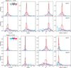 |
Fig. 6 Results from simulations of a single model source. The distribution of recovered parameters from uv_fit to the visibilities (panels labelled with UVFIT) and galfit in the image plane (panels labelled with GALFIT) allowed us to measure their respective accuracy in recovering the known intrinsic parameters (dashed vertical lines), including the flux density and structural parameters (Re, q, and n). We present two examples using a Spergel profile as the input source: Re/θb = 0.4, q = 0.75, PA = 30°, v = −0.6 (two top panels), and Re/θb = 0.2, q = 0.6, PA = 30°, v = 0.5 (two bottom panels). The distribution of the recovered parameters is color coded by flux density (Stot/σb = 25, 100, and 400, indicated by different colors in the inset panel). The Sérsic indices shown in the UVFIT panels were obtained by converting the best-fit Spergel indices based on Eq. (3). For all parameters, we took into account the conversion from Spergel-based fits to Sérsic-based fits, discussed in Sect. 2 (see Eqs. (3) and (4)), to remove any underlying systematics coming from the difference in the profiles. |
4.1.1 Flux measurements
The left panels of Fig. 7 show the median relative difference between the recovered and input flux densities given by (Sout − Sin)/Sin plotted against Sérsic n (converted from input v using Eq. (3)). For both methods, there is a positive bias in recovering the flux density leading to an overestimation of the flux. The magnitude of this bias depends on both the S/N (Stot/σb) and the source extension (Re/θb).
For the image plane fitting with galfit, our simulations show that even relatively compact sources with Stot/σb of 25 exhibit systematic errors >20% in the recovered flux densities. Large-sized sources with Re/θb = 0.7 can be boosted by approximately 60% of flux density at an S/N of approximately 25. In contrast, the systematic biases of flux densities measured from the uυ fitting are much smaller, with a mean value of ~5% at the faintest S/N ~ 25.
4.1.2 Size measurements
In terms of size estimates, the uυ-plane method shows significantly smaller systematic offsets than image-plane measurements (see the panels in the second column of Fig. 7). Both methods have higher relative biases on Re than flux density. In general, both methods tend to overestimate Re for sources with a low Stot/σb.
In the image plane, for a compact, faint (Stot/σb = 25) source with a disk-like profile, the Re can be overestimated by up to 70%. On the other hand, the visibility-based Re is, on average, overestimated by only about 15% for the same model source.
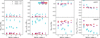 |
Fig. 7 Relative difference between the input and measured parameters, flux density, effective radius, axis ratio, and Sérsic index (from left to right) obtained from Spergel fits to the uυ-plane (top panels) and Sérsic fits in the image plane using galfit (bottom panels) in our simulations plotted as a function of light concentration (i.e., Sérsic index) for various Stot/σb and source sizes. Sources with a size of Ré/θb = 0.2 and 0.7 are marked by a diamond and a triangle, respectively, while the inset panel’s color bar shows the different input flux densities. The error bars denote the interquartile range of the distribution divided by the square root of the number of simulations. |
4.1.3 Axis ratio measurements
In Fig. 7 (third-column panels), the accuracy of recovering the axis ratio q is compared by profile fitting in the image plane and uυ-plane, respectively. Both the image-based and visibility-based measurements tend to systematically underestimate the recovered q in most cases, but again the bias is much stronger in the image plane. In addition, the accuracy of q estimates is influenced by the size of galaxies, with the highest bias occurring for the most compact sources.
4.1.4 Sersic index measurements
For image-based measurements, the Sérsic n estimate is often biased toward a lower value in most cases (Fig. 7, fourth column). There is a significant increase in systematic offsets of measured Sérsic n as light concentration increases. In other words, the difference in estimating n becomes large at low S/N and when the galaxy profile is steep. For the faintest source (i.e., Stot/σb = 25) with a de Vaucouleurs-like profile in the simulation, the Sérsic n estimates can be underestimated by about 70%. The underestimation goes down to 30% when the source becomes less centrally concentrated with a disk-like profile.
While the visibility-based concentration index shows systematic offsets at low S/N, it is still much less biased than the image-based one. The bulk of the error on n estimates obtained from the uυ-plane is limited to within about 20% or less. We emphasize that for very compact sources at the lowest S/N, the estimates of n tend to be higher than the true value. Furthermore, the systematic error in the fit is greater for sources with an exponential profile than those with a steeper profile.
4.2 Comparison of the relative measurement uncertainty
Apart from systematic biases, it is also important to evaluate the scatter of the measurements, both in the uυ-plane and in the image plane, to verify if any of the two returns better measurements with lower scatter. In order to evaluate such relative measurement uncertainty, we used the scatter of the distribution of recovered values evaluated as the median absolute deviation (MAD) of the data around the true value (i.e., input mock value) converted to σ using σ =1.48×MAD, which is what is expected for a normal distribution. The use of MAD is preferred in order to be less dependent on outliers while capturing the bulk of the spread in the sample. By defining the deviation with respect to the true value, the measurement bias was also taken into account when evaluating the overall uncertainty in the measurements. Figure 8 compares the scatter of measurements obtained from the uυ-fitting with those obtained in the image plane for each key structural parameter.
Again, we found that the random uncertainties in all structure parameter recoveries are systematically larger for image-based estimates than those obtained by visibility analysis. The median scatter ratio of measurements obtained from the uυ-fitting to those obtained from the image-plane fitting for the recovered flux densities is 0.5, while for the recovered effective radius, axis ratio, and Sérsic n, the median scatter ratios are 0.5, 0.6, and 0.5, respectively. We did not find a significant correlation between the scatter ratio and the S/N of the data. These findings are in line with a study that compared the performance of stacking data in the uυ-plane and image plane and found that uυ stacking resulted in a significantly improved accuracy of size estimates, with typical errors less than half compared to image stacking (Lindroos et al. 2015).
We emphasize that the small residual systematics shown in Figs. 2 and 3, inherent in the conversion of Spergel-based parameters of our simulations to Sérsic parameters, only account for a negligible amount of the excess noise coming from galfit (and have no effect at all for the n = 1 case). In conclusion, we find that measurements in the image plane not only are more subject to bias but also return parameters that are more substantially affected by noise compared to those in the uυ-plane.
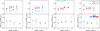 |
Fig. 8 Similar to Fig. 7, but we plot the ratio of the scatter of the measurements derived from Spergel fits in the uυ-plane to that derived from Sérsic fits in the image plane for fitted parameters. From left to right, we show the flux density, effective radius, axis ratio, and Sérsic index as a function of light concentration (i.e., Sérsic index). |
5 Analysis: absolute accuracy of uυ-plane modeling and reliability of uncertainties
In this section, we focus on the performances of the Spergel model fitting in GILDAS uv_fit. We analyze its accuracy in retrieving intrinsic galaxy morphological parameters and verify the reliability of parameter errors returned by the code. In addition, we evaluate the presence of correlations between fitted parameters in the presence of noise.
5.1 Recoverable signal-to-noise ratio for fitted parameters in the uυ -plane
We checked the achievable accuracy for the parameter estimates from Spergel fits in the uυ-plane by computing the ratio of the uncertainties of the parameter estimates to the input mock value given by σ(para)/para. The uncertainties of the parameter estimates, σ(para), can be evaluated as 1.48×MAD, as discussed in Sect. 4.2.
In Fig. 9, the accuracy of the parameter estimates is shown to vary with the S/N of the data. The parameters estimated were flux density, size, axis ratio, and Sérsic index. To enhance the readability of the figure, only Spergel models with an exponential (v = 0.5) profile and steep profile with v = −0.7 (close to a de Vaucouleurs profile) were considered. These models are shown in the panels between the second and fifth rows. We note that for other cases where the Spergel index was assumed to be between v = 0.5 and −0.7, the measurements were found to be either within or close to the values obtained from the above two cases. Therefore, the results presented in Fig. 9 can be considered representative of the Spergel model.
Figure 9 shows that the uncertainties in measuring galaxy shape parameters, such as size and Spergel index, are significantly larger than those for flux density. The most difficult parameter to estimate is the Spergel index. The uncertainty in estimating the Spergel index can be as high as 70% for model sources with a S tot/σb of 25 or lower, suggesting that the measurement of the Spergel index can be highly uncertain. As the S tot/σb increases to 50, the accuracy of Spergel index estimates significantly improves, with a median value of σ(n)/n of 0.36, which we consider as the bare minimum to define a meaningful estimate. At S tot/σb of 50, the uncertainties of the flux density, size, and axis ratio are significantly smaller, with median values of 9%, 18%, and 22% of estimates, respectively. To obtain a meaningful and reliable profile fitting result with the Spergel model in the uυ-plane, our simulations strongly suggest that a S tot/σb of at least 50 is required.
In addition, we found that the accuracy of both the flux density and size is lower for simulated data with a steep profile compared to the model data with a flat profile. On average, the accuracy of flux densities and sizes for the galaxy with an exponential profile (v = 0.5) is 50% higher than those of the galaxy with a de Vaucouleurs-like profile (v = −0.7). However, we note that the measurements of Spergel v tend to be less accurate for smaller sources (Re/θb ⩽0.2), compared to the larger sources in the data. We also found that both the flux densities and sizes of the small-sized sources are more accurately measured, with a typical factor of about 40%. The differences in the accuracy of parameter estimates imply that all the fitted parameters are interrelated.
5.2 Reliability of parameter uncertainties from UVFIT
In Fig. 10, we compare the average value of parameter errors in simulated galaxies to the posterior scatter of the recovered distributions in order to explore their reliability. We found that in most cases, the uncertainties of parameters measured from the Spergel profile fitting are underestimated, although typically within a factor of two. The underestimation is generally less important for steep profiles (v = −0.7) than for disks (v = 0.5) and for extended versus compact galaxies. At each flux S/N bin, the ratio between the error obtained from simulations and the median of the error measured by uv_fit for the whole set of simulated sources is in the range of 1.4–1.9, 2.0–3.2, 1.9–2.5, and 1.4–1.6 (see the black bars in Fig. 10), with a mean value of 1.6, 2.5, 2.1, and 1.5 for the parameter estimates of flux density, effective radius, axis ratio, and Spergel index, respectively.
5.3 Covariance of Spergel model fitted parameters
In this section, we examine the covariance between fitted parameters estimated from uv_fit using a Spergel model. The top panels in Fig. 11 show the correlations between the fitted parameters, which are flux density S tot/σb, effective radius Re/θb, axis ratio q, and Spergel index v, for a simulated dataset with an input Stot/σb of 100, Re/θb of 0.2, q of 0.6, and v of −0.5, respectively. In this case, the Spearman correlation coefficient, which is calculated by dividing the covariance by the intrinsic scatter of each parameter, shows weak correlations (|ρ| ≲ 0.3) between fitted parameters of size, axis ratio, and v, while moderate correlations (|ρ| ~ 0.5) were found between the flux density and both v and size.
The bottom part of Fig. 11 summarizes the pair wise correlation coefficients calculated for all the datasets in our simulation. Generally, we found that the correlation between variables becomes more prominent as the S/N increases, except for the correlation between flux density and size. For sources that are significantly more compact than the beam (Re/θb < 0.2), the correlation between the flux density and measured source size is weaker when the source is detected with a high S/N. We did not find any significant correlation between q and other parameters. This indicates that the measured axis ratios are almost independent of these parameters.
There is a positive correlation between flux density and Sérsic n (anti-correlated with Spergel v), indicating that sources with higher measured Sérsic n tend to have a larger flux density. In addition, a strong positive correlation was seen between flux density and size, except for very compact sources with Re/θb of 0.1, where the correlation is relatively weak. This means that sources for which sizes are overestimated have a tendency to also be boosted in flux density.
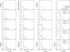 |
Fig. 9 Relative accuracy of the uυ-based parameter estimates, flux density, effective radius, axis ratio, and Sérsic index (from left to right) given by cr(para)/para. Here, σ(para) is the uncertainties of the parameter estimates distribution and is calculated as 1.48×MAD, as a function of the S/N of flux density. The top panels show the results derived from fits with an elliptical Gaussian (orange) and circular Gaussian (green) model, while the results from a Spergel model uυ fit with input Re/θb of 0.1, 0.2, 0.4, and 0.7 are shown in panels from the second to fifth rows, respectively. We only display results for the cases with a Spergel index of 0.5 and −0.7 from our simulation. For other cases with a Spergel index between v = 0.5 and −0.7, the results were found to be within or close to those shown in the panels between the second and fifth rows. The dashed vertical lines represent the threshold of S tot/σb of 50. |
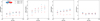 |
Fig. 10 Comparison between the errors obtained from the scatter of the distribution of parameter estimates and the errors estimated by uv_fit at each fit in our simulation as a function of the S/N of flux density. The fitted parameters, from left to right, are flux density, effective radius, axis ratio, and Spergel index. The scatter of the parameter estimates distribution is calculated as σ = 1.48×MAD. Simulated sources with a size of Re/θb = 0.2 (diamond) and 0.7 (triangle) are presented and color coded by the Spergel v. The black bars represent the median value of the ratio between the error in each fitted parameter obtained from simulations and the median of the error measured by uv_fit at each flux S/N bin for the simulated sources in this work. |
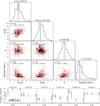 |
Fig. 11 Correlations between the fitted parameters obtained from Spergel profile fitting in the uυ-plane. Top: corner plots showing the covariances between the free parameters modeled in the Spergel profile fitting. The example model source has a flux density of Stot/σb = 100, a size of Re/θb = 0.2, an axis ratio of q=0.6, and a Spergel index of v = −0.5. The shaded density histograms show the two-parameter distributions with the Spearman rank correlation coefficient and p-value marked in each panel. The one-dimensional histograms at the top of each column represent the individual parameter distributions, annotated with the median values. The boundaries of the 25th and 75th percentiles of the distribution are plotted as dashed lines, while the blue vertical lines show the true values. Bottom: Spearman’s rank correlation coefficients of the two-parameter pairs as a function of source size. The points are color coded by the input flux density. |
6 Discussion
The results presented in the previous sections demonstrate that studying galaxy morphologies in the uυ-plane leads to better performance than imaging the data and then using galfit to study morphologies in the image plane. This approach offers exciting possibilities for studying morphologies of galaxies in star-formation rate tracers. However, there are several issues that merit discussion.
6.1 On the differences between Spergel and Sérsic profiles
A comparison between the Spergel and Sérsic profiles showed that the Spergel model has a steeper core and faster declining wings compared to the Sérsic model (see Figs. 1 and A.1), except for the case of Spergel v =0.5, which is equivalent to an exponential profile (Sérsic n=1). The question of whether Spergel or Sérsic models provide better fits to actual galaxies remains open and requires future investigation. The current available data quality may not be sufficient to determine a clear preference between the two functional forms in absolute terms. For the time being, and with the typical data available, we deem the two functional forms to be equivalent.
Converting a Spergel index to a Sérsic one (as well as Re and total flux) requires knowledge of the intrinsic size of the galaxy and the angular resolution of the observations. In the case of this study, the angular resolution was determined by the synthesized beam of the interferometric data. We believe this requirement also applies implicitly to optical observations. When a Sérsic index is derived from optical data, it applies to the range of scales actually observed in the data. It may not apply beyond the observed scales by definition. It is possible that a somewhat different Spergel and Sérsic index might be recovered when re-observing the same galaxy with a much different surface brightness sensitivity.
It is also relevant to question whether the differences in the profiles at the outer and inner ranges could affect the systematic biases of the parameter estimates, particularly for a steep profile. Along these lines, considering that we have simulated Spergel models and then fitted them with galfit in the image plane, one might wonder if the underperformance of galfit in the image plane could be simply related to the discussed differences between the Spergel and Sérsic models.
As already mentioned throughout the description of the results in the previous section, we believe that the argument can be dismissed, but it’s worth recalling the key evidence here. Based on the bottom panels of Fig. 7, the simulations with the highest S/N (400 in this case) show that any average bias in Sérsic modeling vanishes or becomes strongly reduced, as expected by construction (Eq. (3)), showing that any residual systematics beyond our conversions do not have a measurable impact. The systematic differences in the recovered profile parameters (Re and Sérsic n, crucially) are in fact strongly S/N dependent and are therefore mostly an effect of noise (rather than arising from structural differences). Additionally, Fig. 8 shows that the excess noise in parameter recovery from image plane fitting is not a function of S/N, while the systematic deviations between the profiles are expected to become more evident at the highest S/N. Also important, Fig. 8 shows that an entirely consistent situation is seen for the n = 1 case, which is fully identical in shape to a Spergel v of 0.5.
Figure 12 extends this point further by showing the performance comparison of uv_fit versus galfit in the case of Gaussian sources and PSF models. In this case, we directly simulated these shapes in the uυ-plane, which are not Spergel models, and there is no shape difference with respect to the model fitted by galfit. However, the overall behavior is qualitatively the same as in Figs. 7 and 8. There are stronger biases in the image plane (top panels), and the effective noise is also much higher there (lower panels).
6.2 On the origin of the poor performances in the image plane with GALFIT on interferometric data
It has already been shown that ignoring the noise correlation in interferometric images can lead to a significant underestimation of the statistical uncertainty of the results (e.g., Tsukui et al. 2023). To test this idea further, we carried out aperture photometry as an alternative to galfit for point-source simulations. Aperture photometry is one of the techniques used to measure flux density in astronomical observations, which is also used in interferometric images (e.g., Lang et al. 2019; Gómez-Guijarro et al. 2022). We note that, for extended sources, there is an added complication of correcting for flux losses, and this technique has the limitation of not allowing for the estimation of morphological parameters. However, it is well defined for flux density measurements of point sources.
Figure 13 shows the systematic bias and the measurement uncertainty on the recovery of the flux density for point sources using different fitting methodologies, namely, uv_fit with a point source model, galfit with a PSF profile that is identical to the dirty beam of the simulated data, and aperture photometry. The latter was performed with an aperture radius equal to the circularized radius of the beam size and at the position returned by the galfit PSF fitting. It is clear that the flux density estimates obtained through aperture photometry are fully consistent with those measured in the uυ-plane, with a similar level of accuracy in the estimates. Both of these methods exhibit smaller systematic errors and scatters when compared to fitting with a PSF model using galfit. In a way, aperture photometry measurements, being fairly basic and raw, are not fooled by false coherence in the signal induced by correlation, and they return the full S/N performances in the limiting case of point-like emission (Fig. 13-right).
6.3 Warnings against dataset cleaning in view of morphological measurements
It is common practice to perform deconvolution of low-frequency radio interferometric data in order to remove strong sidelobes from bright sources in very large fields, a process known as “cleaning”. We emphasize that in ALMA and NOEMA observations, the FOV is tiny compared to the radio observations, and the source density is basically always manageable, so cleaning can generally be safely avoided. Cleaning, as with any deconvolution approach, is a model-dependent process that in most implementations arbitrarily interpolates the observed source with a superposition of point sources whose sidelobes are then subtracted from the data using the dirty beam. Due to its arbitrariness and its approximation of real sources as multiple point sources, it is clearly not ideal for the analysis of morphological profiles of galaxies. Finally, we emphasize that the cleaning process does not remove correlations in the signal in the image plane, which are due to Fourier transforming the visibilities.
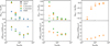 |
Fig. 12 Comparison of profile fitting of Gaussian and PSF models in the uυ-plane and the image plane. Top: relative difference between recovered and input parameters of flux density (left), size (middle), and axis ratio (right). The recovered parameters were obtained from fitting with an elliptical Gaussian (orange), a circular Gaussian (green), and a point (blue) source model using uv_fit (open symbols) and galfit (solid symbols). Bottom: similar to the top panels, but we plot the ratio of measurement uncertainty derived from galfit in the image plane to that obtained from uv_fit in the uυ-plane. The measurement uncertainties are estimated as σ = 1.48×MAD. |
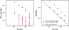 |
Fig. 13 Simulation results of the flux density bias (left) and relative uncertainty of measurement on the recovery of flux density (right) for point sources using uv_fit (red), galfit (black), and aperture photometry (blue) in the image-plane fitting, as a function of the flux S/N. The error bars in the left panel represent the standard error on the mean. The dashed line in the right panel is a 1:−1 line. |
6.4 The cost of using Spergel: Recommendations
To investigate the morphologies of galaxies observed in interferometric images, Spergel modeling directly in the uυ-plane should be the preferred approach. However, a high S/N of at least 50, and ideally much more, is required to perform a Spergel fit that meaningfully constrains the Spergel index, as we have previously commented based on Fig. 9. This requirement is similar to optical observations of galaxies and their galfit modeling, where a high S/N, on order of 100, is needed to attempt derivation of a Sérsic index (van der Wei et al. 2014; Magnelli et al. 2023).
These considerations should be extended further to include other parameters of interest, such as the size or even the flux density. These parameters are easier to derive and require less S/N compared to a Spergel and Sérsic index. However, there is a tension between extracting a meaningful measure from the data and ensuring an unbiased measure. It is important to determine the best approach in balancing these factors.
The top panel of Fig. 9 provides information on the uncertainties in flux density, size, and axis ratio for Gaussian models as a function of their S/Ns. By comparing this information to the bottom panels, one can make a decision between a less complex (Gaussian) fit and a more complex (Spergel) fit to a given dataset. For example, Gaussian fits can provide size uncertainties of about 20% down to an S/N (Stot/σb) of 20, whereas Spergel fits do not offer the same level of accuracy at lower S/Ns. Similar considerations apply to flux density and axis ratio parameters. In addition, there are no significant differences in the accuracy and uncertainty estimates between circular and elliptical Gaussian models (see Fig. 9 and Fig. 12). This demonstrates that the increase in degrees of freedom in Spergel models leads to greater uncertainty in the measured parameters, including flux density and size.
Figure 14 shows the distribution of the ratio of the size obtained from a Spergel fit to that from a Gaussian fit, measured for a sample of about 100 high-z star-forming galaxies observed with ALMA (Q. Tan et al. in prep.). The median ratio between the Re size obtained from a Spergel fit and the FWHM size obtained from a Gaussian fit is  , where uncertainties correspond to the 16th and 84th percentiles of the distribution. This implies that, in most cases, the FWHM size measured from a Gaussian model can be used as a good approximate of the effective radius using the relation Re=FWBM/2. However, we note that almost all of the outliers with a Re/FWHM ratio far from the median value in Fig. 14 are sources measured with a large Sérsic index n (n > 2; Q. Tan et al., in prep.). This suggests that the difference in size measured from a Gaussian fit and a Spergel fit could be significant when the source has a large Sérsic index.
Finally, to achieve a global optimal solution for the Spergel fit, we recommend utilizing the fitting results obtained from Gaussian or exponential fits as prior knowledge for the initial guesses of each structure parameter. This provides good starting guesses, which helps the solver in achieving convergence and in providing a reasonable level of uncertainty. Such preliminary information will also inform the user about the actual merit of proceeding to a more demanding full-Spergel fit.
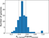 |
Fig. 14 Distribution of the ratio of the size obtained from a Spergel fit to that from a Gaussian fit. The dashed line shows the median of the distribution, while the dotted lines represent the 16th and 84th percentiles of the distribution, respectively. |
6.5 The power of Spergel fitting: a test case
Fitting Spergel models to interferometric data can be complex and requires deep, high S/N data. However, it can also potentially bring powerful insights and enable investigations into new scientific questions.
We aim to demonstrate the potential of our approach by re-examining two cases of published ALMA observations of distant sources that were claimed to contain giant halos surrounding the central galaxies (PACS-787 from Silverman et al. 2018, which includes several co-authors of this paper, and HZ7 from Lambert et al. 2023). These two specific examples are taken from a growing body of results that report the existence of large halos, often observed in [CII]λ1158 µm and other tracers (e.g., Ginolfi et al. 2017; Fujimoto et al. 2019, 2020; Pizzati et al. 2020; Cicone et al. 2021; Herrera-Camus et al. 2021; Jones et al. 2023; Li et al. 2023; Posses et al. 2023; Scholtz et al. 2023, etc.). Extended halos around galaxies are generally interpreted as evidence for accretion, outflows, tidal stripping, or other phenomena affecting distant galaxies. This presents a relevant opportunity for further constraining these processes. However, it is worth considering whether these halos are genuinely different structures from the galaxies or simply the outer scale extension of high Sérsic-index profiles. In many cases, a simple Gaussian fitting was attempted for the central galaxies, and high Sérsic index profiles are well known to display large halos (e.g., Mancini et al. 2010).
We downloaded the data for both datasets as described below. In ALMA Cycle 6, HZ7 was observed with 80 min of on-source integration time in the C43-4 configuration with 47/45 12m antennas in Band 7 (Project 2018.1.01359.S; PI: M. Aravena). The [CII] emission at 303.93 GHz falls into one of four spectral windows, with a native channel width of 15.625 MHz. PACS-787 was observed with high (C40-6, 43 12m antennas with a maximum baseline of 1.1 km) and low (C40-1, 42 12 m antennas with a maximum baseline of 278.9 m) resolution configuration in Band 6 with 19.7 and 10.2 min of on-source integration time in ALMA Cycle 4 (Project 2016.1.01426.S; PI: J. Silverman). The CO(5−4) emission at 228.17 GHz falls into a native channel width of 3.91 MHz in high-resolution observation and 15.62 MHz in low-resolution observation. The calibration targets for the three observations above are J1058+0133 for bandpass, pointing, and flux, and J0948+0022 for phase.
The left panels of Fig. 15 show the dirty images of PACS-787 and HZ7, where emission on large scales of several arcsec (tens of kpc) can be readily seen. We modeled the emission in the uυ-space with simple Spergel profiles. For PACS-787, which contains two galaxies in the process of merging, we used two Spergel components (one for each galaxy), while for HZ7, we used a single Spergel. The Spergel fitting in both cases is able to fully account for the emission from the galaxies, simultaneously reproducing the inner emission and the outer halos. The residuals are clean, and no further components are needed, as shown in the right panels of Fig. 15. For the case of PACS-787, the two Spergel components have v = −0.36 and −0.14, and both have Re/θb ~ 0.7. For HZ7, we found v = −0.42 and Re/θb ~ 1.3. Based on Eq. (3) and Fig. 2, this corresponds to Sérsic n ~ 1.5– 3, which is well above the Gaussian approximation (n = 0.5) and also above the exponential case (n = 1), although not as steep as a de Vacouleurs profile (n = 4).
We have shown that the full emission in these two systems can be fit with a single component model, which raises questions about the interpretation of the outer emission as a halo. Although high Sérsic values indicate the presence of both a central component and a profile extending further out than a disk model, with both smoothly connected, there is no apparent solution of continuity between the inner parts and the outer halos. This is similar to the inner versus outer parts of elliptical galaxies, and therefore suggestions of different physical origins for them are less substantiated.
We emphasize that we have only re-evaluated two cases of halos from the literature (out of many that exist) to exemplify the power of fitting more complex Spergel models to ALMA data. It is beyond the scope of this work to re-analyze all similar observations from the ALMA archive. However, we obviously anticipate that in other cases, the halos might disappear once fitted with a Spergel model. This is not only based on the analysis presented here but also on one of the key results from our forthcoming companion paper (Q. Tan et al., in prep.), which suggests that n > 1 models are required for most ALMA observations of distant galaxies.
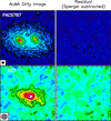 |
Fig. 15 Examples of ALMA images of CO(5−4) and [CII] emission from high-z star-forming galaxies PACS-787 (top) and HZ7 (bottom). Left: ALMA dirty image. Right: residual map with the primary disk component modeled by a single Spergel profile subtracted. The image size is 3.5″ × 3.5″. The synthesized beam (0.15″ × 0.14″ and 0.36″ × 0.35″ for PACS-787 and HZ7, respectively) is presented in the bottom left of the left panels. Contours start from ±2σ and increase by a factor of 1.5. |
7 Conclusions
Spergel’s Bessel function-based luminosity profile provides a good approximation of the Sérsic profile and has the significant advantage of being analytic with a simple Fourier transform. We performed a thorough analysis of the new Spergel fits method for visibilities in the uυ-plane, comparing it to the Sérsic fits for imaged data. Our study was aimed at assessing the effectiveness of the Spergel model fitting based on visibility to galaxy light profiles. We also tested the robustness of the fitting in the υυ-plane by using simpler forms of point and Gaussian profiles. The main findings of our study are as follows:
The conversion of Spergel v into Sérsic n can be closely approximated by a two-variable function
 in the
  -plane. In most cases, we found the differences between the best-fit value and the one measured from simulated data for Sérsic n to be within 10%;
When wishing to compare results from Spergel to Sérsic fitting regarding sizes and total fluxes, similar conversions need to be applied. We find that both the size and total flux estimated by galfit using a Sérsic profile tend to be larger than when using Spergel, as the profile becomes steeper than an exponential profile, while the fitted parameters of axis ratios and PAs are unaffected. The variation of both the ratio of Re,se/Re and S se/Ssp can be described by a similar two-variable function of
 . The best-fit coefficients for the size ratio of Re,se/Re are p1 = 0.00138, p2 = −8.96, p3 = 0.260, p4 = −0.0260, and p5 = 0.996, and for the flux ratio of S se/S sp, they are p1 = 0.00217, p2 = −7.43, p3 = 0.149, p4 = 0.00942, and p5 = 1.00, respectively;
Our MC simulations show that fitting directly in the uυ-plane (rather than imaging the dataset and fitting in the image plane) leads to more consistent and reliable results. The accuracy of fitted structure parameter estimates obtained from uυ-plane fits using a Spergel profile is significantly higher, with smaller systematic errors and scatters on the recovery of parameters. In comparison, image-based measurements obtained from galfit using a Sérsic model tend to have higher systematic biases and larger uncertainties (worse parameter accuracy by a factor of two);
We verified the reliability of the parameter uncertainties returned by GILDAS uv_fit modeling. The parameter uncertainties are generally somewhat underestimated but still correct to better than a factor of two;
We recommend attempting a full-flagged Spergel profile fitting only to sources detected with a Stot/σb of at least 50. This is needed for minimal accuracy and reliability of the Sérsic index (converted from the Spergel index) estimates in the uυ-plane. The corresponding median value of σ(n)/n is 0.36, which we deemed as the minimum threshold for a meaningful and accurate estimate of Sérsic n;
The total flux and size estimates obtained from the Spergel fitting show larger uncertainties at fixed S/N compared to Gaussian and point profile functions, which have fewer degrees of freedom. For the Spergel profile fitting, the uncertainties in measuring galaxy shape parameters were found to be significantly higher than those in measuring flux density. The least accurate constraint requiring the deepest data is the Spergel index;
As a test case, we re-analyzed claims in the literature of the discovery of extended halos surrounding distant galaxies. We find that single Spergel models without any extra added halo can fully explain these observations.
High-quality interferometric data, such as that now routinely obtained from ALMA and NOEMA, allow for the study of the morphology of distant galaxies in their submillimeter band emission. This emission primarily arises from thermal dust and molecular gas, which are closely related to star formation. Fitting a Spergel model in the visibility plane is the preferred method for modeling such emission. In the coming years, this approach should open up a new window of investigation to further the general understanding of the evolution of galaxies.
Acknowledgements
We thank the anonymous referee for constructive suggestions to improve the paper. We are grateful to the IRAM director, Karl Schuster, for the implementation of the Spergel models as part of the GILDAS software package. Q.-H.T. and E.D. would like to dedicate this paper to the memory of late Prof. Yu Gao, who offered kind support for this work. R.I.P. We wish to thank Daizhong Liu for useful discussions. This work has been partly funded by China Scholarship Council. Q.-H.T. acknowledges support from the NSFC (grant nos. 12033004, 12003070, 11803090). C.G.G. acknowledges support from CNES. J.Pe. acknowledges support by the French Agence Nationale de la Recherche through the DAOISM grant ANR-21-CE31-0010 and by the Programme National “Physique et Chimie du Milieu Interstellaire” (PCMI) of CNRS/INSU with INC/INP, co-funded by CEA and CNES. A.P. acknowledges support by an Anniversary Fellowship at University of Southampton and by STFC through grants ST/T000244/1 and ST/P000541/1. This work made use of the following Python libraries: ASTROPY(Astropy Collaboration 2022), NUMPHY(Harris et al. 2020), MATPLOTLIB(Hunter 2007), and EMCEE(Foreman-Mackey et al. 2013).
Appendix A Numerically matching Spergel profiles with Sersic profiles through mathematical simulations
Within a valid range of v (−0.85 ⩽ v ⩽ 4; see Spergel 2010), the matching between Spergel and Sérsic profiles is derived by minimizing the sum of the difference between the Spergel and Sérsic functions over a radial range (see Fig. 1 and Fig. A.1), that is, 2(log((I/Ie)Spergel) − log((I/Ie)Sérsic))2. We used the emcee package (Foreman-Mackey et al. 2013) in Python to perform Markov chain Monte Carlo (MCMC) search for the best fit.
To match with the Sérsic index measured from galfit (see Sect. 2.4), we varied the radial range used for analytic matching and found that the best fit is given by limiting the radius between about 0.01 θb and 2.0 θb for the source sizes (in units of θb, Re/θb) ranging between 0.1 and 2.0. Figure A.2 summarizes the output returned from the Sérsic model versus the true parameters of the profile fits by setting the intensity, Re, and Sérsic index n as free parameters in the MCMC sampler. We found that the relationship between the Sérsic output and Spergel input parameters exhibit similar trends, as seen in Fig. 2 and Fig. 3.
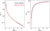 |
Fig. A.1 Comparison of the Sérsic profile with the Spergel profile using mathematical simulations. Left: Surface density profiles for Spergel function (black) compared to the best fit with a Sérsic function (red) through mathematical simulations. Right: Comparison of the integrated surface density profiles for the Sérsic and Spergel functions shown in the left panel. The values of Re,in and Ie,in are held fixed and represent the input parameters in the Spergel profile. |
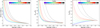 |
Fig. A.2 Comparison between Spergel index v and Sérsic index n (left), the ratio of Re (middle) and total flux (right) obtained from the profile fitting using a Sérsic function to the input value in the Spergel model as a function of Spergel index v. |
Appendix B Details of the three ALMA configurations used to generate simulation data
To generate the data for the simulation, data from three different ALMA array configurations were used in this work. Table B.1 lists the details of each configuration, including the major and minor size of the beam, the PA of the beam, the FOV, and the number of antennas.
Details of the three ALMA array configurations.
Appendix C Details of the elliptical Spergel profile
C.1 Definition and Fourier transform
The circular Spergel profile ( ) located at the phase center (0, 0) is written in Equation (2) as
 (C.1)
(C.1)
where L0 is the total luminosity, R0 is the half-light radius, cv is a tabulated function of v, and
 (C.2)
(C.2)
in which Γ is the Gamma function and Kv(x) is the modified spherical Bessel function of the third kind. Spergel (2010) tabulates the values of cv every 0.05 for a range of v from −0.90 to 0.85. We approximated cv with the following approximation:
 (C.3)
(C.3)
, with
α = −0.403713,
β = −0.228101,
γ = +2.400961.
Figure C.1 compares the tabulated values with our analytical approximation. It results in a relative error of up to 10% for v < −0.6 and less than 1% for v > −0.6.
We used the radio-astronomy convention to define the conjugate coordinates of the angular coordinates (θl;, θm) relative to the projection center of the image as (u, υ) with
 (C.4)
(C.4)
where λ is the wavelength of the observed line. The (θl;, θm) and (u, υ) coordinates are expressed in radian and meter, respectively. In the uυ−plane, the Fourier transform of the circular Spergel profile  (u, υ) can be written as
![Mathematical equation: ${\rm{\tilde \Sigma }}_{(v,0,0)}^{{\rm{circ}}}(u,\upsilon ) = {L_0}{\left[ {1 + {{\left( {2\pi {{{R_0}} \over {{c_v}}}} \right)}^2}\left( {{u^2} + {\upsilon ^2}} \right)} \right]^{ - (1 + v)}}.$](/articles/aa/full_html/2024/04/aa47255-23/aa47255-23-eq21.png) (C.5)
(C.5)
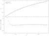 |
Fig. C.1 Comparison between tabulated values of the cv function with an analytical approximation. |
Noting (Rmaj, Rmin) the major and minor half-light radii and ϕ the PA of the elliptical Spergel profile, we yielded the following generalization:
![Mathematical equation: ${\rm{\tilde \Sigma }}_{(v,0,0)}^{{\rm{elli}}}(u,v) = {L_0}{\left[ {1 + {{r_{{\rm{maj}}}^2u_{{\rm{rot}}}^2 + r_{{\rm{min}}}^2v_{{\rm{rot}}}^2} \over {c_v^2}}} \right]^{ - (1 + v)}},$](/articles/aa/full_html/2024/04/aa47255-23/aa47255-23-eq22.png) (C.6)
(C.6)
where (urot, υrot) are the coordinates of the uυ-plane rotated by −ϕ in order to bring the major axis along the urot axis, that is,
 (C.7)
(C.7)
 (C.8)
(C.8)
and (rmaj, rmin) are the reduced major and minor half-light radii, that is,
 (C.9)
(C.9)
An additional phase term appears when the Spergel profile is centered at an offset (θl0,θm0) with respect to the phase center:
![Mathematical equation: ${\rm{\tilde \Sigma }}_{\left( {v,{\theta _{l0}},{\theta _{m0}}} \right)}^{{\rm{elli}}}(u,\upsilon ) = {\rm{\tilde \Sigma }}_{(v,0,0)}^{{\rm{elli}}}(u,\upsilon )\exp \left[ {2i\pi \left( {u{\theta _{l0}} + \upsilon {\theta _{m0}}} \right)} \right].$](/articles/aa/full_html/2024/04/aa47255-23/aa47255-23-eq26.png) (C.10)
(C.10)
C.2 Partial derivatives
In order to differentiate the elliptical Spergel profile, we first rewrote it as
![Mathematical equation: ${\rm{\tilde \Sigma }}_{\left( {v,{\theta _{l0}},{\theta _{m0}}} \right)}^{{\rm{elli}}}(u,\upsilon ) = {L_0}{[g(u,\upsilon )]^{ - (1 + v)}}p(u,\upsilon ),$](/articles/aa/full_html/2024/04/aa47255-23/aa47255-23-eq27.png) (C.11)
(C.11)
with
 (C.12)
and
![Mathematical equation: $p(u,\upsilon ) = \exp \left[ {2i\pi \left( {u{\theta _{l0}} + \upsilon {\theta _{m0}}} \right)} \right].$](/articles/aa/full_html/2024/04/aa47255-23/aa47255-23-eq29.png) (C.13)
(C.13)
The derivative with respect to the luminosity is
![Mathematical equation: ${{\partial {\rm{\tilde \Sigma }}_{\left( {v,{\theta _{l0}},{\theta _{m0}}} \right)}^{{\rm{elli}}}} \over {\partial {L_0}}}(u,\upsilon ) = {[g(u,\upsilon )]^{ - (1 + v)}}p(u,\upsilon ).$](/articles/aa/full_html/2024/04/aa47255-23/aa47255-23-eq30.png) (C.14)
(C.14)
The derivatives with respect to the offset from the phase center are
 (C.15)
and
 (C.16)
The derivatives with respect to the major and minor half-light radius are
![Mathematical equation: $\matrix{ {\,\,\,\,\,\,{{\partial {\rm{\tilde \Sigma }}_{\left( {v,{\theta _{l0}},{\theta _{m0}}} \right)}^{{\rm{elli}}}} \over {\partial {R_{{\rm{maj}}}}}}\left( {u,\upsilon } \right)} \hfill \cr { = - {L_0}\left( {2\pi {{2\,{r_{{\rm{maj}}}}u_{{\rm{rot}}}^2} \over {c_v^2}}} \right)} \hfill \cr {\,\,\,\,\,\, \times (v + 1)\,{{[g(u,\upsilon )]}^{ - (v + 2)}}p(u,\upsilon )} \hfill \cr } $](/articles/aa/full_html/2024/04/aa47255-23/aa47255-23-eq33.png) (C.17)
(C.17)
and
![Mathematical equation: $\matrix{ {\,\,\,\,\,\,{{\partial {\rm{\tilde \Sigma }}_{\left( {v,{\theta _{l0}},{\theta _{m0}}} \right)}^{{\rm{elli}}}} \over {\partial {R_{{\rm{min}}}}}}\left( {u,\upsilon } \right)} \hfill \cr { = - {L_0}\left( {2\pi {{2\,{r_{{\rm{min}}}}\upsilon _{{\rm{rot}}}^2} \over {c_v^2}}} \right)} \hfill \cr {\,\,\,\,\,\, \times (v + 1)\,{{[g(u,\upsilon )]}^{ - (v + 2)}}p(u,\upsilon ).} \hfill \cr } $](/articles/aa/full_html/2024/04/aa47255-23/aa47255-23-eq34.png) (C.18)
(C.18)
The derivative with respect to the PA is
![Mathematical equation: $\matrix{ {\,\,\,\,\,\,{{\partial {\rm{\tilde \Sigma }}_{\left( {v,{\theta _{l0}},{\theta _{m0}}} \right)}^{{\rm{elli}}}} \over {\partial \phi }}\left( {u,\upsilon } \right)} \hfill \cr { = - {L_0}\left( {{{2\left( {\,r_{{\rm{maj}}}^2 - r_{\min }^2} \right)u_{{\rm{rot}}}^2{\upsilon _{{\rm{rot}}}}} \over {c_v^2}}} \right)} \hfill \cr {\,\,\,\,\,\, \times (v + 1)\,{{[g(u,\upsilon )]}^{ - (v + 2)}}p(u,\upsilon ).} \hfill \cr } $](/articles/aa/full_html/2024/04/aa47255-23/aa47255-23-eq35.png) (C.19)
(C.19)
Finally, the derivative with respect to the Spergel index is
![Mathematical equation: $\matrix{ {\,\,\,\,\,\,{{\partial {\rm{\tilde \Sigma }}_{\left( {v,{\theta _{l0}},{\theta _{m0}}} \right)}^{{\rm{elli}}}} \over {\partial v}}\left( {u,\upsilon } \right)} \hfill \cr { = {\rm{\tilde \Sigma }}_{\left( {v,{\theta _{l0}},{\theta _{m0}}} \right)}^{{\rm{elli}}}\left( {u,\upsilon } \right) \times } \hfill \cr {\,\,\,\,\,\,\left[ {\left( {v + 1} \right){{2\left( {r_{{\rm{maj}}}^2u_{{\rm{rot}}}^2 + r_{{\rm{min}}}^2\upsilon _{{\rm{rot}}}^2} \right)} \over {gc_v^3}}\left( {\beta + {\gamma \over {v + 2}}} \right) - \log g} \right].} \hfill \cr } $](/articles/aa/full_html/2024/04/aa47255-23/aa47255-23-eq36.png) (C.20)
(C.20)
References
- Astropy Collaboration (Price-Whelan, A. M., et al.) 2022, ApJ, 935, 167 [NASA ADS] [CrossRef] [Google Scholar]
- Baes, M., & Gentile, G. 2011, A&A, 525, A136 [NASA ADS] [CrossRef] [EDP Sciences] [Google Scholar]
- Barro, G., Kriek, M., Pérez-González, P. G., et al. 2016, ApJ, 827, L32 [NASA ADS] [CrossRef] [Google Scholar]
- Chen, C.-C., Gao, Z.-K., Hsu, Q.-N., et al. 2022, ApJ, 939, L7 [NASA ADS] [CrossRef] [Google Scholar]
- Cibinel, A., Le Floc’h, E., Perret, V., et al. 2015, ApJ, 805, 181 [CrossRef] [Google Scholar]
- Cicone, C., Mainieri, V., Circosta, C., et al. 2021, A&A, 654, L8 [NASA ADS] [CrossRef] [EDP Sciences] [Google Scholar]
- Ciotti, L., & Bertin, G. 1999, A&A, 352, 447 [NASA ADS] [Google Scholar]
- Condon, J. J. 1997, PASP, 109, 166 [NASA ADS] [CrossRef] [Google Scholar]
- Conselice, C. J. 2014, ARA&A, 52, 291 [CrossRef] [Google Scholar]
- Cutler, S. E., Whitaker, K. E., Mowla, L. A., et al. 2022, ApJ, 925, 34 [NASA ADS] [CrossRef] [Google Scholar]
- Elbaz, D., Leiton, R., Nagar, N., et al. 2018, A&A, 616, A110 [NASA ADS] [CrossRef] [EDP Sciences] [Google Scholar]
- Foreman-Mackey, D., Hogg, D. W., Lang, D., & Goodman, J. 2013, PASP, 125, 306 [Google Scholar]
- Fudamoto, Y., Oesch, P. A., Schouws, S., et al. 2021, Nature, 597, 489 [CrossRef] [Google Scholar]
- Fudamoto, Y., Smit, R., Bowler, R. A. A., et al. 2022, ApJ, 934, 144 [NASA ADS] [CrossRef] [Google Scholar]
- Fujimoto, S., Ouchi, M., Kohno, K., et al. 2018, ApJ, 861, 7 [Google Scholar]
- Fujimoto, S., Ouchi, M., Ferrara, A., et al. 2019, ApJ, 887, 107 [Google Scholar]
- Fujimoto, S., Silverman, J. D., Bethermin, M., et al. 2020, ApJ, 900, 1 [Google Scholar]
- Garthwaite, P. H., Jolliffe, I. T., & Jones, B. 1995, Statistical Inference (London: Prentice Hall Europe) [Google Scholar]
- Ginolfi, M., Maiolino, R., Nagao, T., et al. 2017, MNRAS, 468, 3468 [CrossRef] [Google Scholar]
- Gómez-Guijarro, C., Elbaz, D., Xiao, M., et al. 2022, A&A, 658, A43 [NASA ADS] [CrossRef] [EDP Sciences] [Google Scholar]
- Gómez-Guijarro, C., Magnelli, B., Elbaz, D., et al. 2023, A&A, 677, A34 [NASA ADS] [CrossRef] [EDP Sciences] [Google Scholar]
- Guilloteau, S., & Lucas, R. 2000, ASP Conf. Ser., 217, 299 [Google Scholar]
- Gullberg, B., Swinbank, A. M., Smail, I., et al. 2018, ApJ, 859, 12 [Google Scholar]
- Gullberg, B., Smail, I., Swinbank, A. M., et al. 2019, MNRAS, 490, 4956 [Google Scholar]
- Harris, C. R., Millman, K. J., van der Walt, S. J., et al. 2020, Nature, 585, 357 [NASA ADS] [CrossRef] [Google Scholar]
- Häussler, B., McIntosh, D. H., Barden, M., et al. 2007, ApJS, 172, 615 [Google Scholar]
- Herrera-Camus, R., Förster Schreiber, N., Genzel, R., et al. 2021, A&A, 649, A31 [NASA ADS] [CrossRef] [EDP Sciences] [Google Scholar]
- Hiemer, A., Barden, M., Kelvin, L. S., Häußler, B., & Schindler, S. 2014, MNRAS, 444, 3089 [NASA ADS] [CrossRef] [Google Scholar]
- Hodge, J. A., Swinbank, A. M., Simpson, J. M., et al. 2016, ApJ, 833, 103 [Google Scholar]
- Hodge, J. A., Smail, I., Walter, F., et al. 2019, ApJ, 876, 130 [Google Scholar]
- Hogg, D. W., & Lang, D. 2013, PASP, 125, 719 [NASA ADS] [CrossRef] [Google Scholar]
- Hoyos, C., den Brok, M., Verdoes Kleijn, G., et al. 2011, MNRAS, 411, 2439 [Google Scholar]
- Hunter, J. D. 2007, Comput. Sci. Eng., 9, 90 [NASA ADS] [CrossRef] [Google Scholar]
- Iono, D., Yun, M. S., Aretxaga, I., et al. 2016, ApJ, 829, L10 [Google Scholar]
- Jiménez-Andrade, E. F., Magnelli, B., Karim, A., et al. 2019, A&A, 625, A114 [EDP Sciences] [Google Scholar]
- Jones, G. C., Maiolino, R., Carniani, S., et al. 2023, MNRAS, 522, 275 [NASA ADS] [CrossRef] [Google Scholar]
- Kalita, B. S., Daddi, E., Bournaud, F., et al. 2022, A&A, 666, A44 [NASA ADS] [CrossRef] [EDP Sciences] [Google Scholar]
- Kartaltepe, J. S., Rose, C., Vanderhoof, B. N., et al. 2023, ApJ, 946, L15 [NASA ADS] [CrossRef] [Google Scholar]
- Lambert, T. S., Posses, A., Aravena, M., et al. 2023, MNRAS, 518, 3183 [Google Scholar]
- Lang, P., Schinnerer, E., Smail, I., et al. 2019, ApJ, 879, 54 [Google Scholar]
- Lange, R., Moffett, A. J., Driver, S. P., et al. 2016, MNRAS, 462, 1470 [NASA ADS] [CrossRef] [Google Scholar]
- Le Bail, A., Daddi, E., Elbaz, D., et al. 2023, A&A, submitted, [arXiv:2307.07599] [Google Scholar]
- Li, J., Emonts, B. H. C., Cai, Z., et al. 2023, ApJ, 950, 180 [CrossRef] [Google Scholar]
- Lindroos, L., Knudsen, K. K., Vlemmings, W., Conway, J., & Martí-Vidal, I. 2015, MNRAS, 446, 3502 [NASA ADS] [CrossRef] [Google Scholar]
- Magnelli, B., Gómez-Guijarro, C., Elbaz, D., et al. 2023, A&A, 678, A83 [NASA ADS] [CrossRef] [EDP Sciences] [Google Scholar]
- Mancini, C., Daddi, E., Renzini, A., et al. 2010, MNRAS, 401, 933 [NASA ADS] [CrossRef] [Google Scholar]
- Martí-Vidal, I., Pérez-Torres, M. A., & Lobanov, A. P. 2012, A&A, 541, A135 [NASA ADS] [CrossRef] [EDP Sciences] [Google Scholar]
- Martí-Vidal, I., Vlemmings, W. H. T., Muller, S., & Casey, S. 2014, A&A, 563, A136 [Google Scholar]
- Mazure, A., & Capelato, H. V. 2002, A&A, 383, 384 [NASA ADS] [CrossRef] [EDP Sciences] [Google Scholar]
- Moriondo, G., Cimatti, A., & Daddi, E. 2000, A&A, 364, 26 [NASA ADS] [Google Scholar]
- Nelson, E. J., van Dokkum, P. G., Förster Schreiber, N. M., et al. 2016, ApJ, 828, 27 [Google Scholar]
- Pannella, M., Elbaz, D., Daddi, E., et al. 2015, ApJ, 807, 141 [Google Scholar]
- Pavesi, R., Sharon, C. E., Riechers, D. A., et al. 2018, ApJ, 864, 49 [Google Scholar]
- Peng, C. Y., Ho, L. C., Impey, C. D., & Rix, H.-W. 2002, AJ, 124, 266 [Google Scholar]
- Peng, C. Y., Ho, L. C., Impey, C. D., & Rix, H.-W. 2010, AJ, 139, 2097 [Google Scholar]
- Pignatelli, E., Fasano, G., & Cassata, P. 2006, A&A, 446, 373 [NASA ADS] [CrossRef] [EDP Sciences] [Google Scholar]
- Pizzati, E., Ferrara, A., Pallottini, A., et al. 2020, MNRAS, 495, 160 [Google Scholar]
- Posses, A. C., Aravena, M., González-López, J., et al. 2023, A&A, 669, A46 [NASA ADS] [CrossRef] [EDP Sciences] [Google Scholar]
- Press, W. H., Teukolsky, S. A., Vetterling, W. T., & Flannery, B. P. 1992, Numerical Recipes in C, 2nd edn. (Cambridge: Cambridge University Press) [Google Scholar]
- Puglisi, A., Daddi, E., Liu, D., et al. 2019, ApJ, 877, L23 [Google Scholar]
- Puglisi, A., Daddi, E., Valentino, F., et al. 2021, MNRAS, 508, 5217 [NASA ADS] [CrossRef] [Google Scholar]
- Roueff, A., Gerin, M., Gratier, P., et al. 2021, A&A, 645, A26 [NASA ADS] [CrossRef] [EDP Sciences] [Google Scholar]
- Rujopakarn, W., Daddi, E., Rieke, G. H., et al. 2019, ApJ, 882, 107 [NASA ADS] [CrossRef] [Google Scholar]
- Rujopakarn, W., Williams, C. C., Daddi, E., et al. 2023, ApJ, 948, L8 [NASA ADS] [CrossRef] [Google Scholar]
- Scholtz, J., Maiolino, R., Jones, G. C., & Carniani, S. 2023, MNRAS, 519, 5246 [NASA ADS] [CrossRef] [Google Scholar]
- Sersic, J. L. 1968, Atlas de Galaxias Australes (Cordoba, Argentina: Observatorio Astronomico) (Cordoba, Argentina: Observatorio Astronomico) [Google Scholar]
- Shibuya, T., Ouchi, M., & Harikane, Y. 2015, ApJS, 219, 15 [Google Scholar]
- Silverman, J. D., Daddi, E., Rujopakarn, W., et al. 2018, ApJ, 868, 75 [Google Scholar]
- Smail, I., Dudzevičiūtė, U., Stach, S. M., et al. 2021, MNRAS, 502, 3426 [NASA ADS] [CrossRef] [Google Scholar]
- Spergel, D. N. 2010, ApJS, 191, 58 [NASA ADS] [CrossRef] [Google Scholar]
- Stoica, P., & Moses, R. 2005, Spectral Analysis of Signals (New Jersey: Prentice Hall) [Google Scholar]
- Stuber, S. K., Schinnerer, E., Williams, T. G., et al. 2023, A&A, 676, A113 [NASA ADS] [CrossRef] [EDP Sciences] [Google Scholar]
- Tacchella, S., Carollo, C. M., Renzini, A., et al. 2015, Science, 348, 314 [NASA ADS] [CrossRef] [Google Scholar]
- Tacchella, S., Carollo, C. M., Förster Schreiber, N. M., et al. 2018, ApJ, 859, 56 [Google Scholar]
- Tadaki, K.-I., Genzel, R., Kodama, T., et al. 2017, ApJ, 834, 135 [NASA ADS] [CrossRef] [Google Scholar]
- Tortorelli, L., & Mercurio, A. 2023, Front. Astron. Space Sci., 10, 51 [NASA ADS] [CrossRef] [Google Scholar]
- Tsukui, T., Iguchi, S., Mitsuhashi, I., & Tadaki, K. 2023, J. Astron. Telescopes Instrum. Syst., 9, 018001 [NASA ADS] [Google Scholar]
- Valentino, F., Daddi, E., Puglisi, A., et al. 2020, A&A, 641, A155 [NASA ADS] [CrossRef] [EDP Sciences] [Google Scholar]
- van der Wel, A., Franx, M., van Dokkum, P. G., et al. 2014, ApJ, 788, 28 [Google Scholar]
- Wang, T., Schreiber, C., Elbaz, D., et al. 2019, Nature, 572, 211 [Google Scholar]
- Wuyts, S., Förster Schreiber, N. M., van der Wel, A., et al. 2011, ApJ, 742, 96 [NASA ADS] [CrossRef] [Google Scholar]
- Xiao, M. Y., Elbaz, D., Gómez-Guijarro, C., et al. 2023, A&A, 672, A18 [NASA ADS] [CrossRef] [EDP Sciences] [Google Scholar]
The model sources were created with an extremely high S/N to ensure a robust galfit measurement
In practice, this is done by fitting to the empty data a model with all parameters fixed and a negative flux. The residual image will then have the desired (positive) model added.
All Tables
All Figures
|
Fig. 1 Comparison of surface density profiles (left) and the cumulative distributions (right) for Sérsic (solid lines) and Spergel (dashed lines) functions. The light profile with a Sérsic index of 0.5, 1, 2, 4, and 5 and a Spergel index of 0.85, 0.5, −0.3, −0.6, and −0.7 is shown in different colors. By definition, Re, contains half of the integrated galaxy light. |
| In the text | |
|
Fig. 2 Comparison of Sérsic and Spergel indices. The data (crosses) in the top panel represent the galfit Sérsic indices measured for sources created with the input Spergel model for a range of v values from −0.7 to 0.5 and for different source effective radii (expressed in terms of the FWHM of the synthesized beam, Re/θb) ranging from 0.1 to 2.0. The solid curves in the top panel denote the best-fit empirical relation between Spergel v and galfit Sérsic n, depending on Re/θb, as expressed by Eq. (3). The lower panel displays normalized residuals to the proposed relation. |
| In the text | |
|
Fig. 3 Similar to Fig. 2 but showing the ratio of effective radii (left) and total fluxes (right) obtained from fitting Sérsic models to simulated galaxies created using Spergel profiles (crosses). The data are plotted as a function of their Spergel index. The solid curves denote the best-fit empirical relations as expressed by Eq. (4). The bottom panels show the normalized residuals to the best fit, which are largely within 10%. |
| In the text | |
|
Fig. 4 Example of an empty dataset used for our simulations. Left: noise map. The source emission (which was close to the phase center) was subtracted from the visibility data. The dashed white circle represents the primary beam (i.e., the FOV) of the dataset. Right: histogram of pixel values within the primary beam. The red line represents the best-fitting Gaussian model. The fit suggests that the noise data is at least approximately Gaussian. |
| In the text | |
|
Fig. 5 Example of a simulated source generated with a Spergel profile of Stot/σb = 50, Re/θb = 0.4, axis ratio of q = 0.75, PA = 30°, and Spergel index of v = −0.6. From left to right: the dirty image (top-left), dirty beam (PSF used for convolution in galfit; bottom-left), best-fit source models convolved with the dirty beam (middle), and residuals after subtracting the model source (right). The model source and the model-subtracted residual shown in the top and bottom rows were derived from the uv_fit and galfit fits, respectively. Each image cutout is 9″ × 9″. The contours start from 2σ and increase in steps of 4σ. White crosses mark the best-fit source position obtained from uv_fit. |
| In the text | |
|
Fig. 6 Results from simulations of a single model source. The distribution of recovered parameters from uv_fit to the visibilities (panels labelled with UVFIT) and galfit in the image plane (panels labelled with GALFIT) allowed us to measure their respective accuracy in recovering the known intrinsic parameters (dashed vertical lines), including the flux density and structural parameters (Re, q, and n). We present two examples using a Spergel profile as the input source: Re/θb = 0.4, q = 0.75, PA = 30°, v = −0.6 (two top panels), and Re/θb = 0.2, q = 0.6, PA = 30°, v = 0.5 (two bottom panels). The distribution of the recovered parameters is color coded by flux density (Stot/σb = 25, 100, and 400, indicated by different colors in the inset panel). The Sérsic indices shown in the UVFIT panels were obtained by converting the best-fit Spergel indices based on Eq. (3). For all parameters, we took into account the conversion from Spergel-based fits to Sérsic-based fits, discussed in Sect. 2 (see Eqs. (3) and (4)), to remove any underlying systematics coming from the difference in the profiles. |
| In the text | |
|
Fig. 7 Relative difference between the input and measured parameters, flux density, effective radius, axis ratio, and Sérsic index (from left to right) obtained from Spergel fits to the uυ-plane (top panels) and Sérsic fits in the image plane using galfit (bottom panels) in our simulations plotted as a function of light concentration (i.e., Sérsic index) for various Stot/σb and source sizes. Sources with a size of Ré/θb = 0.2 and 0.7 are marked by a diamond and a triangle, respectively, while the inset panel’s color bar shows the different input flux densities. The error bars denote the interquartile range of the distribution divided by the square root of the number of simulations. |
| In the text | |
|
Fig. 8 Similar to Fig. 7, but we plot the ratio of the scatter of the measurements derived from Spergel fits in the uυ-plane to that derived from Sérsic fits in the image plane for fitted parameters. From left to right, we show the flux density, effective radius, axis ratio, and Sérsic index as a function of light concentration (i.e., Sérsic index). |
| In the text | |
|
Fig. 9 Relative accuracy of the uυ-based parameter estimates, flux density, effective radius, axis ratio, and Sérsic index (from left to right) given by cr(para)/para. Here, σ(para) is the uncertainties of the parameter estimates distribution and is calculated as 1.48×MAD, as a function of the S/N of flux density. The top panels show the results derived from fits with an elliptical Gaussian (orange) and circular Gaussian (green) model, while the results from a Spergel model uυ fit with input Re/θb of 0.1, 0.2, 0.4, and 0.7 are shown in panels from the second to fifth rows, respectively. We only display results for the cases with a Spergel index of 0.5 and −0.7 from our simulation. For other cases with a Spergel index between v = 0.5 and −0.7, the results were found to be within or close to those shown in the panels between the second and fifth rows. The dashed vertical lines represent the threshold of S tot/σb of 50. |
| In the text | |
|
Fig. 10 Comparison between the errors obtained from the scatter of the distribution of parameter estimates and the errors estimated by uv_fit at each fit in our simulation as a function of the S/N of flux density. The fitted parameters, from left to right, are flux density, effective radius, axis ratio, and Spergel index. The scatter of the parameter estimates distribution is calculated as σ = 1.48×MAD. Simulated sources with a size of Re/θb = 0.2 (diamond) and 0.7 (triangle) are presented and color coded by the Spergel v. The black bars represent the median value of the ratio between the error in each fitted parameter obtained from simulations and the median of the error measured by uv_fit at each flux S/N bin for the simulated sources in this work. |
| In the text | |
|
Fig. 11 Correlations between the fitted parameters obtained from Spergel profile fitting in the uυ-plane. Top: corner plots showing the covariances between the free parameters modeled in the Spergel profile fitting. The example model source has a flux density of Stot/σb = 100, a size of Re/θb = 0.2, an axis ratio of q=0.6, and a Spergel index of v = −0.5. The shaded density histograms show the two-parameter distributions with the Spearman rank correlation coefficient and p-value marked in each panel. The one-dimensional histograms at the top of each column represent the individual parameter distributions, annotated with the median values. The boundaries of the 25th and 75th percentiles of the distribution are plotted as dashed lines, while the blue vertical lines show the true values. Bottom: Spearman’s rank correlation coefficients of the two-parameter pairs as a function of source size. The points are color coded by the input flux density. |
| In the text | |
|
Fig. 12 Comparison of profile fitting of Gaussian and PSF models in the uυ-plane and the image plane. Top: relative difference between recovered and input parameters of flux density (left), size (middle), and axis ratio (right). The recovered parameters were obtained from fitting with an elliptical Gaussian (orange), a circular Gaussian (green), and a point (blue) source model using uv_fit (open symbols) and galfit (solid symbols). Bottom: similar to the top panels, but we plot the ratio of measurement uncertainty derived from galfit in the image plane to that obtained from uv_fit in the uυ-plane. The measurement uncertainties are estimated as σ = 1.48×MAD. |
| In the text | |
|
Fig. 13 Simulation results of the flux density bias (left) and relative uncertainty of measurement on the recovery of flux density (right) for point sources using uv_fit (red), galfit (black), and aperture photometry (blue) in the image-plane fitting, as a function of the flux S/N. The error bars in the left panel represent the standard error on the mean. The dashed line in the right panel is a 1:−1 line. |
| In the text | |
|
Fig. 14 Distribution of the ratio of the size obtained from a Spergel fit to that from a Gaussian fit. The dashed line shows the median of the distribution, while the dotted lines represent the 16th and 84th percentiles of the distribution, respectively. |
| In the text | |
|
Fig. 15 Examples of ALMA images of CO(5−4) and [CII] emission from high-z star-forming galaxies PACS-787 (top) and HZ7 (bottom). Left: ALMA dirty image. Right: residual map with the primary disk component modeled by a single Spergel profile subtracted. The image size is 3.5″ × 3.5″. The synthesized beam (0.15″ × 0.14″ and 0.36″ × 0.35″ for PACS-787 and HZ7, respectively) is presented in the bottom left of the left panels. Contours start from ±2σ and increase by a factor of 1.5. |
| In the text | |
|
Fig. A.1 Comparison of the Sérsic profile with the Spergel profile using mathematical simulations. Left: Surface density profiles for Spergel function (black) compared to the best fit with a Sérsic function (red) through mathematical simulations. Right: Comparison of the integrated surface density profiles for the Sérsic and Spergel functions shown in the left panel. The values of Re,in and Ie,in are held fixed and represent the input parameters in the Spergel profile. |
| In the text | |
|
Fig. A.2 Comparison between Spergel index v and Sérsic index n (left), the ratio of Re (middle) and total flux (right) obtained from the profile fitting using a Sérsic function to the input value in the Spergel model as a function of Spergel index v. |
| In the text | |
|
Fig. C.1 Comparison between tabulated values of the cv function with an analytical approximation. |
| In the text | |
Current usage metrics show cumulative count of Article Views (full-text article views including HTML views, PDF and ePub downloads, according to the available data) and Abstracts Views on Vision4Press platform.
Data correspond to usage on the plateform after 2015. The current usage metrics is available 48-96 hours after online publication and is updated daily on week days.
Initial download of the metrics may take a while.