| Issue |
A&A
Volume 683, March 2024
|
|
|---|---|---|
| Article Number | A99 | |
| Number of page(s) | 12 | |
| Section | The Sun and the Heliosphere | |
| DOI | https://doi.org/10.1051/0004-6361/202347843 | |
| Published online | 11 March 2024 | |
Electron moments derived from the Mercury Electron Analyzer during the cruise phase of BepiColombo
1
IRAP, CNRS-UPS-CNES, Toulouse, France
e-mail: This email address is being protected from spambots. You need JavaScript enabled to view it.
2
University of Tokyo, Kashiwa, Japan
3
Institute of Space and Astronautical Science, Japan Aerospace Exploration Agency, Sagamihara, Japan
4
University of Pisa, Pisa, Italy
5
Department of Space and Climate Physics, University College of London, London, UK
6
Department of Earth and Space Science, Graduate School of Science, Osaka University, Osaka, Japan
7
Institut für Geophysik und extraterrestrische Physik, Technische Universität Braunschweig, Braunschweig, Germany
8
Institut für Weltraumforschung, Österreichische Akademie der Wissenschaften, Graz, Austria
9
Faculty of Natural Sciences, Department of Physics, Imperial College London, London, UK
10
Laboratoire d’Etudes Spatiales et d’Instrumentation en Astrophysique, Observatoire de Paris, Université PSL, CNRS, Sorbonne Université, Univ. Paris-Diderot, Sorbonne Paris-Cité, France
11
Swedish Institute of Space Physics, Uppsala, Sweden
Received:
31
August
2023
Accepted:
14
November
2023
Abstract
Aims. We derive electron density and temperature from observations obtained by the Mercury Electron Analyzer on board Mio during the cruise phase of BepiColombo while the spacecraft is in a stacked configuration.
Methods. In order to remove the secondary electron emission contribution, we first fit the core electron population of the solar wind with a Maxwellian distribution. We then subtract the resulting distribution from the complete electron spectrum, and suppress the residual count rates observed at low energies. Hence, our corrected count rates consist of the sum of the fitted Maxwellian core electron population with a contribution at higher energies. We finally estimate the electron density and temperature from the corrected count rates using a classical integration method. We illustrate the results of our derivation for two case studies, including the second Venus flyby of BepiColombo when the Solar Orbiter spacecraft was located nearby, and for a statistical study using observations obtained to date for distances to the Sun ranging from 0.3 to 0.9 AU.
Results. When compared either to measurements of Solar Orbiter or to measurements obtained by HELIOS and Parker Solar Probe, our method leads to a good estimation of the electron density and temperature. Hence, despite the strong limitations arising from the stacked configuration of BepiColombo during its cruise phase, we illustrate how we can retrieve reasonable estimates for the electron density and temperature for timescales from days down to several seconds.
Key words: plasmas / instrumentation: detectors / methods: data analysis
© The Authors 2024
 Open Access article, published by EDP Sciences, under the terms of the Creative Commons Attribution License (https://creativecommons.org/licenses/by/4.0), which permits unrestricted use, distribution, and reproduction in any medium, provided the original work is properly cited.
This article is published in open access under the Subscribe to Open model. This email address is being protected from spambots. You need JavaScript enabled to view it. to support open access publication.
1. Introduction
BepiColombo is the third scientific mission to explore the planet Mercury. This joint mission of the European Space Agency (ESA) and the Japan Aerospace Exploration Agency (JAXA) was launched on October 19, 2018. During its cruise phase, BepiColombo is composed of three stacked platforms: the Mercury Transfer Module (MTM), the Mercury Planetary Orbiter (MPO), and the Mio spacecraft (Mercury Magnetospheric Orbiter, MMO; Murakami et al. 2020). In addition, Mio is protected from the intense radiation of the Sun by the Magnetospheric Orbiter Sunshield and Interface Structure (MOSIF). MPO and Mio both carry a large scientific payload dedicated to studying the internal structure, physical properties, and surface composition and evolution of Mercury, as well as the dynamics of its small magnetosphere (Benkhoff et al. 2021).
The harsh thermal environment and the complexity of the orbit transfer from Earth make Mercury the least explored of the telluric planets. Mariner 10 flew by Mercury three times in 1974 and 1975 and, among other results, characterized for the first time its intrinsic magnetic field. Forty years later, the MErcury Surface, Space ENvironment, GEochemistry, and Ranging (MESSENGER) spacecraft conducted the first orbital study of Mercury from 2011 until 2014, and detailed in particular the interaction of the planet with the solar wind (SW) thanks to the Energetic Particle and Plasma Spectrometer that measured energetic particles accelerated by the magnetosphere together with low-energy ions coming from the Hermean surface (Andrews et al. 2007).
In order to further reveal the structure and dynamics of the magnetosphere of Mercury and its interaction with the SW, the Mercury Plasma Particle Experiment (MPPE; Saito et al. 2021) was mounted on the Mio spacecraft. MPPE includes several instruments: the Energetic Neutral Atom imager (ENA), the Mass Spectrum Analyzer (MSA), the High-Energy Particle detectors for ions (HEP-ion) and electrons (HEP-e), the Mercury Ion Analyzer (MIA), and the two Mercury Electron Analyzers (MEA 1 and 2, shown in Fig. 1) that will detect electrons for the first time in the Mercury orbit over a low-energy range (from 3 eV to 26 keV).
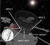 |
Fig. 1. View of the Mio spacecraft with the MEA 1 and 2 sensors during the cruise phase of BepiColombo. The sensors are surrounded by MOSIF (shown in transparency here). The location and field of view of the MEA 1 channels is also represented. Channels 6 and 7 are unobstructed and face the free space, while channel 0 for example is totally obstructed. |
During the cruise phase of BepiColombo, the instruments are turned on for in-flight calibration, which provides opportunities for scientific studies as well. To date, MEA 1 has already accumulated data for more than three months in total (all available time periods are shown in Table A.3). As Fig. 1 shows, MEA 1 and 2 are located close to the MPO and MOSIF surfaces (a few tens of centimeters). Hence, MEA 1 and 2 have a strongly reduced field of view (FoV) and most of their sectors are obstructed (for a detailed description of the MEA 1 and 2 sensors, see Sauvaud et al. 2010 and Saito et al. 2021).
In addition, electrostatic analyzers like MEA have a distorted FoV for low-energy charged particles when the spacecraft surfaces remain negatively or positively charged (Bergman et al. 2020; Guillemant et al. 2017). For example, in the magnetosphere of the Earth, spacecraft in geostationary orbits can charge to several thousand negative volts during magnetic substorms (Matéo-Vélez et al. 2018) and primarily in the postmidnight sector (Sarno-Smith et al. 2016), whereas spacecraft in the SW typically can charge to a few positive volts (Guillemant et al. 2017; Lai & Tautz 2006).
Spacecraft charging strongly affects the determination of plasma moments, especially those of solar wind electrons. For instance, a positive spacecraft potential will accelerate electrons, and hence can shift the electron energy distribution function (EEDF) toward higher energies. In addition, secondary electrons emitted from the spacecraft’s charged surfaces can be re-collected and can contaminate the EEDF. It is therefore necessary to remove the secondary electron contribution in order to obtain the most accurate estimation of the plasma moments (Lewis et al. 2008; Rymer 2004; Génot & Schwartz 2004; Lavraud & Larson 2016). On board BepiColombo we expect that MEA 1 and 2 will suffer from strong secondary electron contamination owing to the presence of MOSIF close to their locations.
Even though BepiColombo is in a stacked configuration during its cruise phase, MEA 1 and 2 have been frequently turned on during several solar wind campaigns as well as dedicated planetary flybys. In this paper we present and discuss the derivation of electron density and temperature from the analysis of MEA 1 observations. In Sect. 2 we describe the effects related to spacecraft charging and the methods that we use in order to properly analyze MEA data and derive the most accurate electron moments. In Sect. 3 we use observations obtained during two particular time periods when Solar Orbiter and BepiColombo were close to each other in order to compare our estimates of the electron moments. In Sect. 4 we discuss the statistical validity of the electron moments deduced from all available BepiColombo MEA observations by comparing them with the studies of Dakeyo et al. (2022) and Sun et al. (2022). Finally, in Sect. 5 we discuss the overall performance of MEA 1 during the cruise phase of BepiColombo, and conclude on all the caveats potentially affecting the accuracy of its scientific products derived while the mission is in stacked configuration.
2. Surface charging, data processing, and removing secondary electrons
2.1. Basics of surface charging
Any object immersed in a plasma is going to experience surface charging (Whipple 1981), which means that the surface of a satellite has an electric potential that is different from that of the plasma. In space we usually set the plasma potential Φp = 0, which means that any other potential, for example that of the spacecraft Φsc, is defined relative to Φp. Around the Earth a spacecraft can experience a negative potential (typically in the shadow region) or a positive potential (in the sunlight). During very energetic events like magnetic substorms, a spacecraft can experience negative potentials of several thousand volts. Typically, scientific spacecraft traveling through the SW have potentials varying between 0 and +10 volt (Matéo-Vélez et al. 2018; Sarno-Smith et al. 2016).
Classical processes related to plasma-surface interactions in space include photo-emission (PE), secondary electron emission under electron (SEEE) or ion (SEEI) impact, or backscattered electrons (BEs). In the current equation, Φsc reaches a stationary state when the sum of all currents on the spacecraft is equal to zero. All the main currents to be considered are included in the following current equation:
 (1)
(1)
Here Ie, Ii, ISEEE, ISEEI, IBE, and IPE are the electronic, ionic, SEEE, SEEI, BE, and PE currents, respectively. The different electronic populations emitted by the surfaces of a spacecraft are considered to follow a Maxwellian energy distribution, with a temperature Tsec of typically 2–3 eV. Each secondary emission process is characterized by its energy-dependent emission yield δ which gives the number of emitted electrons per impacting particle (electrons, ions, or photons). In addition, the secondary emission depends on the nature of the material and on its surface state (Tolias 2014; Walker et al. 2008). In the case of SEEE, a surface charges positively when δ > 1. In addition, SEEE is more important for a material when the maximum δmax is the highest and δ > 1 is on the widest energy interval. In the case of SEEI, it is comparable to SEEE, but because δ > 1 for several keV amu−1 (Lakits et al. 1990), SEEI is often neglected. In the SW, IPE is responsible for the typically observed positive Φsc (Sarno-Smith et al. 2016).
When an object immersed in a plasma is composed of different materials, conductive and dielectric, the surfaces can charge to different potentials causing differential charging (Prokopenko & Laframboise 1980). During the cruise phase of BepiColombo, Mio is in the shadow of MOSIF. The outer surface of MOSIF is made of a dielectric fabric, Nextel AF-10 (Tessarin et al. 2010), and has a conductive layer of titanium inside (Stramaccioni et al. 2011), and so we expect that differential charging arises between the inner and outer surfaces of MOSIF. Unfortunately, it is impossible to measure either Φsc (due to the stacked configuration) or the potential of the Nextel surface ΦNextel on the outer surface of MOSIF. If ΦNextel > Φsc, photoelectrons would be re-collected by the outer surface of MOSIF, and MEA 1 would not detect any of them. In this configuration the low-energy part of the EEDF would be dominated by SEEE. On the other hand, if ΦNextel < Φsc, then both PE and SEEE would dominate the low-energy part of the EEDF. In the next subsection we show how we remove these different contributions from MEA measurements and determine their nature.
2.2. Derivation of electron moments and removing of secondary electrons
During the cruise phase of BepiColombo, Mio is always in low-telemetry mode (L-mode). In L-mode, MEA provides different types of data products (Saito et al. 2021) using only 16 energy bins (see Table A.1), in particular including electron omnidirectional fluxes (Et-OMNI), onboard electron velocity moments (VMs), and full 3D electron distribution (3D). In order to derive Et-OMNI (hereafter OMNI), the count rates from all channels are simultaneously integrated for each energy bin. On the contrary, for 3D distribution the electrons are measured in each channel separately. In this work we focus on the MEA 1 sensor because it is the only one that can provide 3D data products. The OMNI data products are not the best ones to use during the cruise phase since many of the MEA 1 and 2 FoV sectors are obstructed by both MOSIF and the presence of the undeployed boom of the magnetometer (MAST-MGF). Therefore, in order to obtain the most accurate moments, we create a virtual channel that uses the maximum count rates between channels 6 and 7 of MEA 1 (which are the sectors with the largest unobstructed FoV during cruise phase) per time step. Then we assume that the main electron population is isotropic, which is a reasonable assumption for the core electron population of the SW (Halekas et al. 2020). Before deriving the electron moments, we need to remove the secondary electrons contributing to the observed count rates at low energies.
2.2.1. Removing the contributions from secondary electrons
Because of MOSIF, the antennas of the Plasma Wave Investigation (PWI) instrument cannot be deployed during the cruise phase of BepiColombo in order to measure Φsc. The classical method to determine the spacecraft potential from electrostatic analyzer measurements consists of identifying a discontinuity in the observed count rates at low energies, which is caused by the secondary electron emitted with enough energy to escape the spacecraft electric sheath. Then, using the Liouville theorem and assuming that the plasma sheath between the spacecraft and the undisturbed plasma is collisionless, it is possible to shift in energy the phase space density (PSD) in order to determine the electron moments (Lavraud & Larson 2016). Here, the stacked configuration of BepiColombo during its cruise phase prevents us from relying on this classical method. First, MOSIF almost completely surrounds the Mio spacecraft. Assuming that the space between Mio and MOSIF is mainly filled by ambient electrons of density 10 cm−3 and temperature of 15 eV, the Debye length λD is ≈9 m. The electrons emitted from the internal surfaces of MOSIF would not be affected by electric fields. Hence, no discontinuity in the count rates measured by MEA at low energies would be detected, and this would not enable us to precisely determine Φsc. Second, the low-telemetry mode of Mio during the cruise phase of BepiColombo restricts MEA to only 16 energy bins, which would reduce drastically the accuracy of such a method.
In order to avoid such limitations, we prefer to apply a different method, which is summarized in Fig. 2. The red solid line represents electron count rates for an original electron spectrum measured on March 11, 2022, at 19:39:40 UTC. We first fit the observed core electron population with a Maxwellian distribution represented by the brown stars. In order to obtain the most accurate fit, we detect the maximum count rate, identified by the vertical pink dotted line. This fit is constrained by six energy bins: two before the identified maximum, the maximum and three after it. We then subtract the Maxwellian fit from the original count rates in order to obtain the residuals represented by the magenta dotted line. We remove from the original energy spectrum the contribution at low energies represented by the transparent pink area. Finally, we reconstruct the corrected energy spectrum by summing the Maxwellian fit with the residuals at high energies represented by the magenta dotted line.
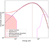 |
Fig. 2. Illustration of the procedure applied to remove the secondary electron emission contribution from a complete electron energy spectrum measured by MEA 1 on March 11, 2022, at 19:39:40 UTC. The red line corresponds to the original count rate, the brown stars are a Maxwellian fit of the original count rate. The magenta dotted lines represent the residuals at low and high energies when the Maxwellian fit has been subtracted from the original count rates. Finally, the brown line shows the reconstructed corrected count rate. |
One limitation of this method is the underlying assumption that electrons are isotropic, which forces us to consider a Maxwellian distribution function instead of a bi-Maxwellian distribution function with temperatures parallel and perpendicular to the magnetic field (Halekas et al. 2020). The ecliptic plane contains the Y-axis of the MPO spacecraft frame (always pointing Sunward so that the MOSIF thermal shield protects the Mio spacecraft) and the Z-axis of the Mio spacecraft frame represented in Fig. 1. The interplanetary magnetic field in its nominal Parker spiral configuration at the distances considered in the present work is mainly oriented toward the Y-axis of the MPO spacecraft frame. As a consequence channels 6 and 7 of the MEA instrument used in this work make an angle of ±45° with respect to the ecliptic plane at maximum, and are typically perpendicular to the interplanetary magnetic field. The limited pitch angle distributions of electrons observed by MEA during the cruise phase of BepiColombo prevent us from detecting anisotropic features on their distribution functions, as reported by Halekas et al. (2020) and Berčič et al. (2019). Now that we have described how we correct energy spectra, we further detail how we derive electron density ne and temperature Te from MEA 3D data products.
2.2.2. Electron moments: Integration method
Mio is a spin-stabilized spacecraft with a period of rotation Tspin = 4 s. The elementary time step is  considering eight channels, 16 azimuthal sectors, and the 16 energy bins used by MEA during the cruise phase of BepiColombo (see Table A.1). Then, for the cruise phase only, we replace all eight channels by our virtual channel, and use
  ms.
ms.
The classical formula used to deduce the density n from the distribution function f is given by
 (2)
(2)
with v the electron velocity, and θ and ϕ the elevation and the azimuthal angles, respectively. Following Nicolaou (2023) we can relate the density to the count rate matrix C from
 (3)
(3)
with GE the energy-dependent geometrical factor, E the electron energy, me the electron mass, and |q| the absolute value of the elementary charge. We assume that an isotropic electron population C does not depend on the elevation angle, but only on the electron energy.
After integrating Eq. (3) over all elevation angles and azimuthal sectors we obtain
 (4)
(4)
where Cr(E) is the count rate integrated over the whole solid angle and fE(E) represents the EEDF. Then we can simply deduce the electronic temperature Te from (Godyak & Demidov 2011):
 (5)
(5)
Here the temperature Te refers to a particle population that reaches the thermodynamical equilibrium, which is described by a Maxwellian distribution. With this method, Te should be considered an effective temperature because fE(E) can deviate from a pure Maxwellian distribution.
Now that the method is established, we can compare the solar wind electron moments deduced with this method from the BepiColombo data to the electron moments derived from Solar Orbiter (SolO) data during their respective second Venus flybys (VFB).
3. BepiColombo and Solar Orbiter encounters at Venus
3.1. The BepiColombo second Venus flyby on August 10, 2021
On August 09 and 10, 2021, SolO and BepiColombo performed their respective second VFB. This represented a unique opportunity for MEA to compare the estimated electronic moments with similar observations obtained simultaneously by SolO in almost the same region of the heliosphere when in the solar wind. SolO includes three instruments relevant to our study: the Proton Alpha Sensor (PAS) and the Electron Analyzer System (EAS) from the Solar Wind Analyzer (SWA) suite (Owen et al. 2020), and the Radio Plasma Wave (RPW) instrument (Maksimovic et al. 2020). PAS and EAS are both electrostatic analyzers, while RPW contains, among other instruments, three electric field antennas.
The configuration of this space encounter is represented in Fig. 3. The upper panel shows the BepiColombo (in purple) and SolO (in blue) trajectories in the XY plane in the Venus Solar Orbital (VSO) coordinate system, from August 10, 2021, 00:00:00 UTC to August 11, 2021, 00:00:00 UTC. The lower panel shows the radial distance between the two spacecraft (in black) and the angle between rBepi and rSolO (in red) in the Heliocentric Inertial (HCI) coordinate system. During this time interval the two spacecraft are almost radially aligned, and are located at a close distance ranging from 225 to 290 Venus radii from each other. This unique two-point measurement configuration is particularly advantageous since the two spacecraft should have observed the same solar wind plasma populations.
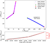 |
Fig. 3. Attitudes of BepiColombo and Solar Orbiter with respect to Venus and the Sun. Upper panel: trajectories of BepiColombo during its second Venus flyby (in purple) and SolO (in blue), in the Venus Sun Orbital (VSO) coordinate system. Each green and red dot represents the starting and ending points of each spacecraft’s trajectory, respectively. Lower panel: radial distance (in Venus radius, 6052 km) between BepiColombo and SolO (in black), and angle θ (in red) between SolO, the Sun, and BepiColombo, in the Heliocentric Inertia (HCI) coordinate system. |
In order to take advantage of this opportunity, we use the proton bulk velocity measured by SolO/PAS to time-shift the magnetic field vector B measured by SolO to the location of BepiColombo. We present the resulting comparison in Fig. 4. The magnetic fields observed by the two spacecraft are almost identical for the chosen time interval. The main difference is due to the Venus bow shock crossing by BepiColombo around 14:00 UTC (Persson et al. 2022), represented by the vertical green dashed line. Since B is “frozen in” to the plasma, the two spacecraft should therefore have observed the same solar wind plasma populations. Persson et al. (2022) also identified the electron foreshock region, and showed that BepiColombo crossed it in less than five minutes. Since the 3D data products of MEA 1 are obtained every 640 s, only one single 3D measurement was obtained within this region; this does not impact the comparison between Solar Orbiter and BepiColombo observations when applied to the whole time interval considered.
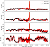 |
Fig. 4. Magnetic field measured by MPO during its second Venus flyby (in red) on August 10, 2021, and the magnetic field measured by SolO and time-shifted (about 1 hour delay) to the location of BepiColombo (in black). From the upper to the lower panel, we respectively compare ∥B∥, Bx, By, and Bz in the VSO coordinate system. The green dotted line indicates the time of the bow shock crossing of the induced magnetosphere of Venus by BepiColombo. |
The upper panel in Fig. 5 represents the time energy spectra of electrons measured by EAS together with the SolO potential ΦSolO measured by RPW (in black). The EAS and RPW data are time-shifted at the location of BepiColombo in order to facilitate the comparison. The lower panel shows MEA 1 energy spectra obtained from our virtual channel during the BepiColombo second Venus flyby. The MEA 3D data product provides one 4 s measurement every 640 s (due to the very limited telemetry downlink rate of Mio during the cruise phase of BepiColombo). The three large data gaps observed are due to wheel off-loadings (WoLs). The virtual channel spectra of MEA 1 do not show exactly the same intensity fluctuations that can be seen on the electron spectra of EAS, in particular around 20–60 eV. As expected, ΦSolO is anti-correlated with the intensity of EAS spectra. The RPW allows an accurate estimation of the electron density ne, RPW, which is anti-correlated to the SolO potential. As explained in Khotyaintsev et al. (2021), ΦSolO has a logarithmic dependence on ne, RPW.
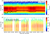 |
Fig. 5. Comparison between electron energy spectrograms measured by EAS and MEA 1. Upper panel: time-energy spectrogram of electron count rates measured by EAS and time-shifted to the location of BepiColombo during its second Venus flyby on August 10, 2021, with the superimposed spacecraft potential of SolO measured by RPW ΦSolO (in black). Lower panel: time-energy spectrogram of electron count rates built with the virtual channel extracted from the MEA 1 3D data products. |
The time-shifted plasma density ne measured with EAS and RPW are displayed in Fig. 6. In order to obtain ne, EAS, the counts below the spacecraft potential measured by RPW were removed, then the PSD was shifted to the cutoff energy of EAS. We observe that ne, RPW and ne, EAS are nearly identical, and therefore we expect ne, MEA1 to match this profile during its Venus flyby, except around the CA where BepiColombo no longer observes the undisturbed solar wind since it crossed the induced magnetosphere of Venus. In the same figure we plot ne, MEA1 calculated by two different methods. The red stars correspond to the density ne calculated by integrating the whole energy spectra without applying any corrections. The blue dots correspond to the density ne determined by integrating the whole energy spectra with the secondary electrons removed, as described in Sect. 2.2.1.
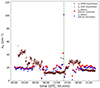 |
Fig. 6. Time evolution of ne (in cm−3) during the VFB on August 10, 2021. The brown triangles and crosses represent ne measured by RPW and EAS respectively, time-shifted to the location of BepiColombo. The red stars represent ne after the integration of the entire electron energy spectra without applying any corrections, while the blue dots represent ne after the integration of the entire electron spectra with the secondary electrons removed. The green dotted line indicates the time of the bow shock crossing of the induced magnetosphere of Venus by BepiColombo. |
Even though the order of magnitude of ne, MEA1 matches the SolO measurements, we observe that MEA 1 does not capture the complete dynamics of the plasma as observed by EAS. Using the 3D velocity distribution functions extracted from the EAS data, we checked and confirmed that the core solar wind electrons are nearly isotropic, as assumed for the derivation of the MEA moments. We suspect that the presence of MOSIF could be responsible for the non-detection of the complete dynamics of the plasma by MEA. We also note that the lower cutoff energy of MEA 1 represents another issue to be accounted for in this case. When ne, RPW is high, Φsc of SolO is low. If Φsc < 3.6 V, the lower part of the PSD cannot be measured by MEA 1, which means that ne, MEA will be underestimated. In addition, a few values of ne are greater after correction (i.e., after secondary electrons have been removed from the electron spectra) compared to the uncorrected density. This may indicate that the Maxwellian model does not always fit the core electron population well. This leads to an overestimation of the density.
Figure 7 represents the temporal evolution of the electron temperature Te. The brown crosses correspond to the EAS measurements, whereas the red stars and blue dots correspond to the electron temperature Te calculated from the MEA measurements by integrating the entire electron energy spectra without applying any corrections and with the secondary electrons removed, respectively. With MEA 1 we retrieve the same order of magnitude for Te as observed by EAS. However, again, we hardly capture the complete temporal dynamics of the plasma.
3.2. Before the Venus flyby: July 8 to 15, 2021
Before the VFB of BepiColombo, MEA 1 was turned on from July 6, 2021, until July 16, 2021. During this time interval, the distance between SolO and BepiColombo decreased from 12.1 × 10⁶ to 11.4 × 10⁶ km, and the angle between rBepi and rSolO in the HCI coordinate system varied from 3° to 2° as we can see in Fig. 8. Using the same method as described above, we can time-shift the SolO measurements to the location of BepiColombo, using the solar wind speed measured by SolO/PAS. The magnetic field observed by BepiColombo and SolO are plotted in Fig. 9 in the HCI coordinate system, which shows ∥B∥, Bx, By, and Bz. The magnetic fields measured by the two spacecraft do not match as nicely as during the VFB time period studied before, but still agree remarkably well on a timescale of a few hours. The observed difference may be due to the larger distance and angular separation between the two spacecraft during this time period compared to the VFB. Hence, we expect the electron moments to agree between the two spacecraft on a similar timescale during this time period.
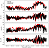 |
Fig. 9. Magnetic field measured by MPO (in red) from July 8 to 15, 2021. Magnetic field measured by SolO (in black) and time-shifted at the location of BepiColombo. From the upper to the lower panel, ∥B∥, Bx, By, and Bz are compared in the HCI coordinate system. |
Figure 10 represents the same comparison of the electron density that we showed in Fig. 6, together with the density of secondary electrons ne, sec (green diamonds), but for this new time interval. We calculate ne, sec by integrating the residual count rate at low energy (see Fig. 2) using Eq. (4). For this time interval SWA is off, and therefore we cannot determine the electron temperature from the Solar Orbiter observations. As a consequence, we only compare ne, MEA with ne, RPW. Independently of the method we use to calculate ne, MEA, the densities overlap for all the time intervals, except between July 13 and July 14, and at the end of the time interval. We observe that both ne, MEA calculated by integrating the whole energy spectra without applying any corrections and calculated with the secondary electrons removed present a good correlation with ne, RPW over the entire time interval. We also note that the secondary electron density seems to be correlated with the SW density, showing that the nature of the secondary emission is likely SEEE. If it was produced by PE, no correlation would be observed. In agreement with the comparison made in Fig. 9, the solar wind dynamics are captured over timescales of days, even if we are only able to retrieve the order of magnitude of ne with MEA.
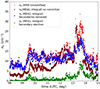 |
Fig. 10. Time evolution of the electron density ne (in cm−3), from July 8 to 15, 2021. The brown triangles represent ne measured by RPW and time-shifted at the location of BepiColombo. The red stars and the blue dots are the density calculated with MEA 1, without and with the secondary electrons removed, respectively. The green diamonds correspond to the density of secondary electrons deduced by integrating the residuals at low energies (see details in the text). |
In Fig. 11 we plot ne, RPW (in cm−3) versus ne, MEA (in cm−3) with (black crosses) and without (green triangles) the secondary electrons removed, respectively. Each dataset is fitted with a linear regression, which can be compared with the gray dotted curve representing ne, RPW = ne, MEA. We find a similar correlation factor between MEA and RPW independently of whether we remove or not the secondary electron emission (r = 0.67 without the correction and r = 0.68 with the correction). This result and the correlation between the secondary and SW electron densities presented in Fig. 10 seem to show that our method is adapted to remove secondary electrons from the electron energy spectra. In order to confirm this interpretation in the next section, we derived electron densities from all the measurements obtained by MEA 1 during the cruise phase of BepiColombo. So far, MEA 1 has accumulated more than three months of data, which allow us to also investigate the variations in electron moment with distance to the Sun.
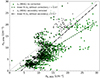 |
Fig. 11. Comparison of the solar wind electron density ne (in cm−3) measured by RPW and by MEA with (black crosses) and without (green triangles) secondary electrons removed. The green dashed line and the black dot-dashed line represent a linear regression fit for the uncorrected and corrected density, respectively. |
4. Density and temperature versus distance to the Sun
In Sect. 3 we showed that even with the limited FoV of MEA 1 during the cruise phase of BepiColombo, we can still capture the order of magnitude for the electron density ne and temperature Te in the solar wind. However, to fully investigate the efficiency of the method applied during the whole cruise phase of BepiColombo, we now determine ne and Te for all the available observations from MEA 1 and study their radial profiles with distance from the Sun. We compare them with the profiles reported by Sun et al. (2022) and Dakeyo et al. (2022) using HELIOS and PSP observations, respectively.
Figure 12 is inspired from Fig. 2d from Sun et al. (2022), where they represent the statistical evolution of the proton density with respect to the distance to the Sun. Here we show the statistical evolution of ne, MEA. The color map represents a 2D distribution of ne, MEA using the integration method after removing the secondary electrons, using 25 bins for the distance and 100 bins for the density. For each distance bin, the density distribution is normalized by its maximum value, where the solid black line links all the density maxima at each distance bin. In Sun et al. (2022) they fitted their proton density distributions extracted from Parker Solar Probe (PSP) measurements with a simple power law, represented here by the black dashed line for comparison. Here we fit the maximum ne variation over distance from the Sun with a similar power law, represented by the blue star dotted line and the purple diamond dotted line; they respectively show the density profiles when the secondary electrons have not been removed and when they have been removed. We observe a good agreement between the fit from Sun et al. (2022) and ours. Even if the method we used to remove the secondary electrons leads to a small underestimation, our radial profile agrees well with the fit from Sun et al. (2022). This underestimation could be explained by the location of MEA 1 (close to MOSIF surfaces) and by the differential charging that should occur between Mio and MOSIF. The low-energy electrons, being more sensitive to small electric fields, can be easily deflected from the detector.
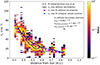 |
Fig. 12. Statistical evolution of the electron density ne (in cm−3) measured by MEA1 with respect to the distance to the Sun. The colormap represents a 2D distribution, with 25 bins for the distance and 100 bins for the density. ne is estimated from MEA by removing the contribution of the secondary electrons. For each distance bin, the density distribution is normalized by its maximum value. The solid black line links all the density maxima at each distance bin. Three power-law fits are represented: the black dashed line, the blue stars, and the purple diamonds for the Sun et al. (2022) fit, ne without the secondary electrons removed, and ne with the secondary electrons removed, respectively. |
The calculation of the electron temperature shows a different result if we remove or not the contribution from the secondary electrons. In Fig. 13 the black dots and the red stars represent Te and its median, respectively, estimated with the secondary electrons removed. The yellow tripods stand for the median of Te estimated without the secondary electrons removed. We also show Te, sec (purple dots) and its median values (dark purple triangles), which is the temperature of the secondary electrons calculated from the residuals at low energies. The profile of Te, sec is discussed in Sect. 5. The median value of Te is calculated over 25 distance bins. The blue gradient crosses, squares, pentagons, and diamonds are temperatures extracted from Dakeyo et al. (2022); they respectively represent Te for SW populations classified by SW speeds: (A) very slow (250 < vSW < 300 km s−1), (B) slow (300 < vSW < 350 km s−1), (C) fast (350 < vSW < 450 km s−1), and (D) very fast (450 < vSW < 600 km s−1). The temperatures comes from PSP observations obtained for 0.12 < rSun < 0.35 AU, and from HELIOS observations obtained for 0.3 < rSun < 0.9 AU.
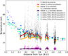 |
Fig. 13. Statistical evolution of the electron temperature Te (in eV) with respect to the distance of the Sun. The black dots, the red stars, and the yellow tripod solid line stand for Te and the median of Te determined with and without the secondary electrons removed, respectively. The purple dots and triangles correspond to Te, sec and its median, determined from integrating the residuals at low energies (see text for more details). The color gradients with crosses, squares, pentagons, and diamonds represent the median Te for four different SW populations (A, B, C, and D), extracted from the PSP and HELIOS missions by Dakeyo et al. (2022). |
Figure 13 shows that the electron temperature Te calculated using our method with the secondary electrons removed agrees remarkably well with those of Dakeyo et al. (2022) down to around 0.4 AU. On the contrary, the electron temperature Te calculated using our method without the secondary electrons removed remains almost constant with distance to the Sun. However, at distances between 0.3 and 0.35 AU, the electron temperature Te from MEA appears underestimated compared to that used in Dakeyo et al. (2022). Since only a limited dataset restricted to three days is obtained by BepiColombo in this region of the heliosphere, this discrepancy may be due to a colder than usual solar wind electron population observed by BepiColombo at that time.
5. Discussion
Figures 12 and 13 show that the method used in this work allows us to retrieve the large-scale variations in the electron density and temperature in the solar wind from MEA observations, despite the complex and atypical configuration of BepiColombo during its cruise phase. However, Figs. 6 and 10 show that we hardly capture the complete temporal dynamics of the plasma. Plasma surface interaction occurring between MOSIF and Mio could be responsible for this limitation. We observe in the energy–time spectrogram of Fig. 5 that the fluctuations of the electron intensities (which can be related to the electronic density fluctuations) disappear above 60 eV. The potential differential charging between the outer and inner surfaces of MOSIF and/or the different surface materials inside MOSIF that surround MEA 1 and 2 may repel or deflect low-energy electrons and reduce the probability of detecting them. These phenomena could occur during the whole cruise phase, which may explain the slight density underestimation observed on the radial profile presented in Fig. 12 compared to that from Sun et al. (2022).
The stacked configuration of BepiColombo strongly constrains the nature of the secondary electrons that we detect with MEA. Figure 14 shows the count rate measured in the shadow of Mercury at closest approach during the third flyby of the planet by BepiColombo on June 19, 2023. We observe two electron populations: one at low energy, corresponding to secondary electrons, and one at hundreds of eV, corresponding to trapped electrons in Mercury’s magnetosphere. Because these observations are obtained when BepiColombo is in the shadow of Mercury, we deduce that the observed secondary electrons are produced by SEEE and confirm that they are not photoelectrons. In order to know if the same process is responsible for the secondary electrons observed during the whole cruise phase, we conduct another statistical study by applying Eq. (4) on both the corrected electron energy spectrum and the residuals at low energies. If photo emission is the main process producing secondary electrons, we should not observe a correlation between the SW electron density ne and the secondary electron density ne, sec. Indeed, PE depends only on the extreme ultraviolet photon intensity. On the contrary, if SEEE dominates, we should observe a strong correlation between ne and ne, sec. Figure 15 represents a 2D histogram of ne, sec versus ne, 3D. All MEA 1 3D data products available to date are used in order to produce a reliable statistic. The red dashed line and the blue dash-dotted line represent respectively a fit from a linear regression and from a repeated median regression (also called Siegel regression; this method is less sensitive to outliers). We note a strong correlation between ne, sec and ne, 3D with r = 0.84, and a strong overlap between the two regression fits. Therefore, we can conclude that the main secondary emission process is SEEE. The derived slope indicates that the ne, sec represents about one-third of the SW electron density.
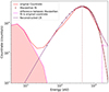 |
Fig. 14. Same as Fig. 2, but recorded in the shadow region of Mercury during the third flyby of BepiColombo, on June 19, 2023, 19:34:00 UTC, at the closest approach. |
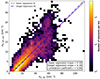 |
Fig. 15. 2D histogram of secondary electron densities versus SW electron densities. The red dashed line and the blue dash-dotted line represent a fit from a linear regression and from a repeated median (Siegel) regression, respectively. |
Finally, we observe that the temporal dynamics are similar for each channel of MEA. In addition, the maximum count rate values observed shifts toward lower energy when we consider channels with an obstructed FoV. This energy shift is due to electron thermalization after they collide with MOSIF and Mio surfaces. Applying Eq. (4) without the secondary electrons removed for the count rate measured by each channel gives electron densities strongly correlated with the densities estimated from the unobstructed channels 6 and 7. If such a strong correlation exists between all the MEA channels, this implies that we could apply a correcting factor on electron densities calculated with the OMNI data products and obtain densities with 4 s time resolution. Therefore, we can reconstruct the OMNI data taking into account the count rates from all the channels provided by the 3D data products and calculating the corresponding electron density ne, 3D-OMNI. Figure 16 shows electron densities ne estimated from 3D data products with the secondary electrons removed versus ne, 3D-OMNI. From the very good correlation obtained, with a coefficient r = 0.94, we could apply a corrective factor of 1.4 for the high time-resolved OMNI densities ne, 3D-OMNI to get closer to the low time-resolved 3D density ne, 3D.
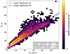 |
Fig. 16. ne, 3D versus ne, 3D-OMNI, both in cm−3. The red dashed line is a linear fit with correlation coefficient of r = 0.94, the blue dash-dotted line is a Siegel regression fit. |
However, there is dispersion around the linear fit. If we simply multiply ne, Omni calculated with the Omni data products by a factor of 1.4, ne, Omni could sometimes be higher or lower than ne, 3D. In order to adjust ne, Omni to ne, 3D without secondary electrons, we subtract ne, 3D-OMNI to ne, 3D. This difference with a time step of 640 s is interpolated for the real Omni data product where the time step is 4 s. Then we interpolate the difference for the time steps (4 s) of all the Omni data products. Finally, we sum the interpolated difference with ne, Omni. We show an example of this method in Fig. 17. The upper and middle panel show respectively an energy count rate spectra obtained with MEA 1 with the Omni data products and our 3D virtual channel. The lower panel shows a comparison between ne, 3D and the shifted values of ne, Omni. For better visibility, the maximum density value at the bow shock crossing is not shown here. Between 10:30 and 13:30 we observe fluctuations of ne, 3D. These variations are correlated with the SW count rate measured in 20–40 eV energy range on the 3D virtual channel spectra. These fluctuations are barely visible in the Omni spectra. Hence, this shifted ne, Omni becomes closely related with the 3D virtual channel that is only open to space, and no longer with the Omni data products.
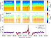 |
Fig. 17. Comparison of Omni and 3D electron energy spectra and the density derived from the 3D and Omni data product. Upper panel: Omni count rate energy spectra measured on August 10, 2021, with MEA 1. Middle panel: 3D virtual channel count rate energy spectra measured on the same day with MEA 1. Lower panel: comparison of the ne, 3D calculated from 3D data product without secondary electrons and ne, Omni shifted at ne, 3D (blue dots and red plus signs, respectively). The vertical green dotted line represents the bow shock crossing. |
The main interest of shifting ne, Omni values is that we can better probe transition regions during a flyby, whereas no 3D data product were available. During the second Venus flyby we find that ne ≈ 180 cm−3 at the bow shock. This method will be of great interest to better describe each magnetic region of Mercury during the last three flybys of BepiColombo.
Despite all the limitations encountered by MEA in the stacked configuration of BepiColombo during its cruise phase, we would like to highlight the very good performance of the instrument. In all cases good orders of magnitude for the electron density and temperature in the solar wind were retrieved locally and statistically, even with only two channels completely open to space and a very narrow FoV. In addition, we were able to recover the plasma dynamics on timescales of days or less. This study therefore gives us confidence that MEA will reach its optimal performance when the Mio spacecraft starts its independent science phase in orbit around Mercury in late 2025. This study, together with the recent study by Griton et al. (2023), will make it possible to cross-calibrate future MEA 1 and 2 measurements with those obtained by the Plasma Wave Investigation (Kasaba et al. 2020) on board Mio.
6. Conclusions
The main objective of this paper was to discuss the performance, limitations, and constraints that apply to MEA observations when deriving electron moments during the cruise phase of BepiColombo. The main difficulty comes from the fact that BepiColombo is in a stacked configuration during its cruise phase, with the thermal shield MOSIF highly reducing the field of view of the MEA instruments on board the Mio spacecraft. In order to overcome this severe limitation we used 3D data products from MEA 1 that have a lower time and energy resolution, and rely only on the two channels of MEA 1 that are unobstructed.
In this paper we developed and applied a method for determining the electron density and temperature of the solar wind plasma from all the MEA 1 observations obtained during the cruise phase of BepiColombo, assuming the observed solar wind electrons are isotropic. We took advantage of two-point close measurements from the BepiColombo and Solar Orbiter missions in order to successfully qualitatively and quantitatively compare the electron moments derived from several instruments, on timescales of days and hours. We confirmed that our derived electron density and temperature are consistent with statistical variations in solar wind parameters derived from the Parker Solar Probe and HELIOS missions. Our analysis revealed, however, that MEA measurements are strongly contaminated at low energies by secondary electron emissions. We illustrated how we can efficiently remove the contributions from those secondary electrons, and we discussed how their contribution impacts our estimation of the electron density and temperature in the solar wind. Finally, we show that the electron density calculated from MEA 3D and the OMNI data products are highly correlated. It may therefore be possible to apply a corrective factor on the densities derived from the MEA OMNI data products in order to increase their time resolution significantly.
Acknowledgments
The authors acknowledge all members of the BepiColombo and Solar Orbiter missions for their unstinted efforts in making them successful. In particular the MEA Team would like to thank Claude Aoustin for managing the technical activities of the instrument development at IRAP. French co-authors acknowledge the support of Centre National d’Etudes Spatiales (CNES, France) to the BepiColombo and Solar Orbiter missions. BepiColombo is a joint space mission between ESA and JAXA. M.P.P.E. is funded by JAXA, CNES, the Centre National de la Recherche scientifique (CNRS, France), the Italian Space Agency (ASI), and the Swedish National Space Agency (SNSA). Solar Orbiter is a space mission of international collaboration between ESA and NASA, operated by ESA. Solar Orbiter Solar Wind Analyser (SWA) data are derived from scientific sensors which have been designed and created, and operated, under funding provided in numerous contracts from the UK Space Agency (UKSA), the UK Science and Technology Facilities Council (STFC), ASI, CNES, CNRS, the Czech contribution to the ESA PRODEX program, and NASA. Solar orbiter SWA work at UCL/MSSL is currently funded under STFC grants ST/T001356/1 and ST/S000240/1. Solar Orbiter magnetometer operations are funded by the UK Space Agency (grant ST/T001062/1). The RPW instrument has been designed and funded by CNES, CNRS, the Paris Observatory, The Swedish National Space Agency, ESA-PRODEX and all the participating institutes. M.R. is funded by a CNES postdoctoral fellowship. M.P. is funded by the European Union’s Horizon 2020 program under grant agreement No 871149 for Europlanet 2024 RI. S.A. is supported by JSPS KAKENHI number: 22J01606. T.S.H. is supported by STFC grant ST/S000364/1. D.H. was supported by the German Ministerium für Wirtschaft und Energie and the German Zentrum für Luft-und Raumfahrt under contract 50 QW1501. The first author M.R. would like to thank Lucile Martinez from Atelier Borderouge, Toulouse, for the preparation of Fig. 1, Jean-Baptiste Dakeyo for kindly providing his dataset of radial temperature profiles, Benoît Lavraud and Quentin Nenon for all useful talks on particle detection and spacecraft charging. The BepiColombo/Mio/MPPE/MEA data presented here are available for download in the Zenodo database at https://zenodo.org/records/10058910. After the proprietary period, the BepiColombo/MPO/MAG data analyzed in this study will be available at the ESA-PSA archive https://archives.esac.esa.int/psa/#!Table%20View/BepiColombo=mission. We used data of the Solar Orbiter MAG, SWA and RPW data, which are publicly available at the Solar Orbiter Archive Repository (https://soar.esac.esa.int/soar/) of the European Space Agency.
References
- Andrews, G. B., Zurbuchen, T. H., Mauk, B. H., et al. 2007, Space Sci. Rev., 131, 523 [CrossRef] [Google Scholar]
- Benkhoff, J., Murakami, G., Baumjohann, W., et al. 2021, Space Sci. Rev., 217, 90 [NASA ADS] [CrossRef] [Google Scholar]
- Berčič, L., Maksimović, M., Landi, S., & Matteini, L. 2019, MNRAS, 486, 3404 [Google Scholar]
- Bergman, S., Stenberg Wieser, G., Wieser, M., Johansson, F. L., & Eriksson, A. 2020, J. Geophys. Res.: Space Phys., 125, e2019JA027478 [Google Scholar]
- Dakeyo, J.-B., Maksimovic, M., Démoulin, P., Halekas, J., & Stevens, M. L. 2022, ApJ, 940, 130 [NASA ADS] [CrossRef] [Google Scholar]
- Génot, V., & Schwartz, S. 2004, Ann. Geophys., 22, 2073 [CrossRef] [Google Scholar]
- Godyak, V., & Demidov, V. 2011, J. Phys. D: Appl. Phys., 44, 233001 [NASA ADS] [CrossRef] [Google Scholar]
- Griton, L., Issautier, K., Moncuquet, M., et al. 2023, A&A, 670, A174 [NASA ADS] [CrossRef] [EDP Sciences] [Google Scholar]
- Guillemant, S., Maksimovic, M., Hilgers, A., et al. 2017, IEEE Trans. Plasma Sci., 45, 2578 [CrossRef] [Google Scholar]
- Halekas, J., Whittlesey, P., Larson, D., et al. 2020, ApJS, 246, 22 [Google Scholar]
- Kasaba, Y., Kojima, H., Moncuquet, M., et al. 2020, Space Sci. Rev., 216, 1 [CrossRef] [Google Scholar]
- Khotyaintsev, Y. V., Graham, D. B., Vaivads, A., et al. 2021, A&A, 656, A19 [NASA ADS] [CrossRef] [EDP Sciences] [Google Scholar]
- Lai, S. T., & Tautz, M. F. 2006, IEEE Trans. Plasma Sci., 34, 2053 [CrossRef] [Google Scholar]
- Lakits, G., Aumayr, F., Heim, M., & Winter, H. 1990, Phys. Rev. A, 42, 5780 [NASA ADS] [CrossRef] [Google Scholar]
- Lavraud, B., & Larson, D. E. 2016, J. Geophys. Res.: Space Phys., 121, 8462 [NASA ADS] [CrossRef] [Google Scholar]
- Lewis, G., André, N., Arridge, C., et al. 2008, Planet. Space Sci., 56, 901 [NASA ADS] [CrossRef] [Google Scholar]
- Maksimovic, M., Bale, S., Chust, T., et al. 2020, A&A, 642, A12 [NASA ADS] [CrossRef] [EDP Sciences] [Google Scholar]
- Matéo-Vélez, J.-C., Sicard, A., Payan, D., et al. 2018, Space Weather, 16, 89 [CrossRef] [Google Scholar]
- Murakami, G., Hayakawa, H., Ogawa, H., et al. 2020, Space Sci. Rev., 216, 113 [CrossRef] [Google Scholar]
- Nicolaou, G. 2023, Ap&SS, 368, 3 [NASA ADS] [CrossRef] [Google Scholar]
- Owen, C., Bruno, R., Livi, S., et al. 2020, A&A, 642, A16 [NASA ADS] [CrossRef] [EDP Sciences] [Google Scholar]
- Persson, M., Aizawa, S., André, N., et al. 2022, Nat. Commun., 13, 7743 [NASA ADS] [CrossRef] [Google Scholar]
- Prokopenko, S., & Laframboise, J. 1980, J. Geophys. Res.: Space Phys., 85, 4125 [NASA ADS] [CrossRef] [Google Scholar]
- Rymer, A. M. 2004, Analysis of Cassini Plasma and Magnetic Field Measurements from 1-7 AU (UK: University of London, University College London) [Google Scholar]
- Saito, Y., Delcourt, D., Hirahara, M., et al. 2021, Space Sci. Rev., 217, 1 [NASA ADS] [CrossRef] [Google Scholar]
- Sarno-Smith, L. K., Larsen, B. A., Skoug, R. M., et al. 2016, Space Weather, 14, 151 [NASA ADS] [CrossRef] [Google Scholar]
- Sauvaud, J.-A., Fedorov, A., Aoustin, C., et al. 2010, Adv. Space Res., 46, 1139 [NASA ADS] [CrossRef] [Google Scholar]
- Stramaccioni, D., Battaglia, D., Schilke, J., & Tessarin, F. 2011, in 41st International Conference on Environmental Systems, 5007 [Google Scholar]
- Sun, W., Dewey, R. M., Aizawa, S., et al. 2022, Science China Earth Sciences (Springer), 1 [Google Scholar]
- Tessarin, F., Battaglia, D., Malosti, T., Stramaccioni, D., & Schilke, J. 2010, in 40th International Conference on Environmental Systems, 6090 [Google Scholar]
- Tolias, P. 2014, Plasma Phys. Control. Fusion, 56, 123002 [NASA ADS] [CrossRef] [Google Scholar]
- Walker, C., El-Gomati, M. M., Assa’d, A., & Zadražil, M. 2008, Scanning, 30, 365 [CrossRef] [Google Scholar]
- Whipple, E. C. 1981, Rep. Prog. Phys., 44, 1197 [NASA ADS] [CrossRef] [Google Scholar]
Appendix A: Tables
In Table A.1 we give the energy tables of MEA 1 for two different science modes (3-300 eV and 3-3,000 eV) used during the cruise phase of BepiColombo. In Table A.2 we give the updated geometrical factors (GFs) used to calculate electron moments from MEA 1 during the cruise phase of BepiColombo. In Table A.3 we list all the available time periods when MEA 1 was turned on in science mode in 2021 and 2022.
Energy tables used by MEA 1 in science mode during the cruise phase of BepiColombo.
Geometrical factors used for MEA 1 during the cruise phase of BepiColombo.
Time periods when MEA 1 was turned on in science mode during the cruise phase of BepiColombo. MFB and VFB stand for Mercury flyby and Venus flyby, respectively.
All Tables
Energy tables used by MEA 1 in science mode during the cruise phase of BepiColombo.
Time periods when MEA 1 was turned on in science mode during the cruise phase of BepiColombo. MFB and VFB stand for Mercury flyby and Venus flyby, respectively.
All Figures
|
Fig. 1. View of the Mio spacecraft with the MEA 1 and 2 sensors during the cruise phase of BepiColombo. The sensors are surrounded by MOSIF (shown in transparency here). The location and field of view of the MEA 1 channels is also represented. Channels 6 and 7 are unobstructed and face the free space, while channel 0 for example is totally obstructed. |
| In the text | |
|
Fig. 2. Illustration of the procedure applied to remove the secondary electron emission contribution from a complete electron energy spectrum measured by MEA 1 on March 11, 2022, at 19:39:40 UTC. The red line corresponds to the original count rate, the brown stars are a Maxwellian fit of the original count rate. The magenta dotted lines represent the residuals at low and high energies when the Maxwellian fit has been subtracted from the original count rates. Finally, the brown line shows the reconstructed corrected count rate. |
| In the text | |
|
Fig. 3. Attitudes of BepiColombo and Solar Orbiter with respect to Venus and the Sun. Upper panel: trajectories of BepiColombo during its second Venus flyby (in purple) and SolO (in blue), in the Venus Sun Orbital (VSO) coordinate system. Each green and red dot represents the starting and ending points of each spacecraft’s trajectory, respectively. Lower panel: radial distance (in Venus radius, 6052 km) between BepiColombo and SolO (in black), and angle θ (in red) between SolO, the Sun, and BepiColombo, in the Heliocentric Inertia (HCI) coordinate system. |
| In the text | |
|
Fig. 4. Magnetic field measured by MPO during its second Venus flyby (in red) on August 10, 2021, and the magnetic field measured by SolO and time-shifted (about 1 hour delay) to the location of BepiColombo (in black). From the upper to the lower panel, we respectively compare ∥B∥, Bx, By, and Bz in the VSO coordinate system. The green dotted line indicates the time of the bow shock crossing of the induced magnetosphere of Venus by BepiColombo. |
| In the text | |
|
Fig. 5. Comparison between electron energy spectrograms measured by EAS and MEA 1. Upper panel: time-energy spectrogram of electron count rates measured by EAS and time-shifted to the location of BepiColombo during its second Venus flyby on August 10, 2021, with the superimposed spacecraft potential of SolO measured by RPW ΦSolO (in black). Lower panel: time-energy spectrogram of electron count rates built with the virtual channel extracted from the MEA 1 3D data products. |
| In the text | |
|
Fig. 6. Time evolution of ne (in cm−3) during the VFB on August 10, 2021. The brown triangles and crosses represent ne measured by RPW and EAS respectively, time-shifted to the location of BepiColombo. The red stars represent ne after the integration of the entire electron energy spectra without applying any corrections, while the blue dots represent ne after the integration of the entire electron spectra with the secondary electrons removed. The green dotted line indicates the time of the bow shock crossing of the induced magnetosphere of Venus by BepiColombo. |
| In the text | |
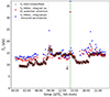 |
Fig. 7. Same as Fig. 6, but for the electron temperature Te (in eV). |
| In the text | |
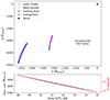 |
Fig. 8. Same as Fig. 3, but from July 8 to 15, 2021. |
| In the text | |
|
Fig. 9. Magnetic field measured by MPO (in red) from July 8 to 15, 2021. Magnetic field measured by SolO (in black) and time-shifted at the location of BepiColombo. From the upper to the lower panel, ∥B∥, Bx, By, and Bz are compared in the HCI coordinate system. |
| In the text | |
|
Fig. 10. Time evolution of the electron density ne (in cm−3), from July 8 to 15, 2021. The brown triangles represent ne measured by RPW and time-shifted at the location of BepiColombo. The red stars and the blue dots are the density calculated with MEA 1, without and with the secondary electrons removed, respectively. The green diamonds correspond to the density of secondary electrons deduced by integrating the residuals at low energies (see details in the text). |
| In the text | |
|
Fig. 11. Comparison of the solar wind electron density ne (in cm−3) measured by RPW and by MEA with (black crosses) and without (green triangles) secondary electrons removed. The green dashed line and the black dot-dashed line represent a linear regression fit for the uncorrected and corrected density, respectively. |
| In the text | |
|
Fig. 12. Statistical evolution of the electron density ne (in cm−3) measured by MEA1 with respect to the distance to the Sun. The colormap represents a 2D distribution, with 25 bins for the distance and 100 bins for the density. ne is estimated from MEA by removing the contribution of the secondary electrons. For each distance bin, the density distribution is normalized by its maximum value. The solid black line links all the density maxima at each distance bin. Three power-law fits are represented: the black dashed line, the blue stars, and the purple diamonds for the Sun et al. (2022) fit, ne without the secondary electrons removed, and ne with the secondary electrons removed, respectively. |
| In the text | |
|
Fig. 13. Statistical evolution of the electron temperature Te (in eV) with respect to the distance of the Sun. The black dots, the red stars, and the yellow tripod solid line stand for Te and the median of Te determined with and without the secondary electrons removed, respectively. The purple dots and triangles correspond to Te, sec and its median, determined from integrating the residuals at low energies (see text for more details). The color gradients with crosses, squares, pentagons, and diamonds represent the median Te for four different SW populations (A, B, C, and D), extracted from the PSP and HELIOS missions by Dakeyo et al. (2022). |
| In the text | |
|
Fig. 14. Same as Fig. 2, but recorded in the shadow region of Mercury during the third flyby of BepiColombo, on June 19, 2023, 19:34:00 UTC, at the closest approach. |
| In the text | |
|
Fig. 15. 2D histogram of secondary electron densities versus SW electron densities. The red dashed line and the blue dash-dotted line represent a fit from a linear regression and from a repeated median (Siegel) regression, respectively. |
| In the text | |
|
Fig. 16. ne, 3D versus ne, 3D-OMNI, both in cm−3. The red dashed line is a linear fit with correlation coefficient of r = 0.94, the blue dash-dotted line is a Siegel regression fit. |
| In the text | |
|
Fig. 17. Comparison of Omni and 3D electron energy spectra and the density derived from the 3D and Omni data product. Upper panel: Omni count rate energy spectra measured on August 10, 2021, with MEA 1. Middle panel: 3D virtual channel count rate energy spectra measured on the same day with MEA 1. Lower panel: comparison of the ne, 3D calculated from 3D data product without secondary electrons and ne, Omni shifted at ne, 3D (blue dots and red plus signs, respectively). The vertical green dotted line represents the bow shock crossing. |
| In the text | |
Current usage metrics show cumulative count of Article Views (full-text article views including HTML views, PDF and ePub downloads, according to the available data) and Abstracts Views on Vision4Press platform.
Data correspond to usage on the plateform after 2015. The current usage metrics is available 48-96 hours after online publication and is updated daily on week days.
Initial download of the metrics may take a while.