| Issue |
A&A
Volume 698, June 2025
|
|
|---|---|---|
| Article Number | A221 | |
| Number of page(s) | 7 | |
| Section | Planets, planetary systems, and small bodies | |
| DOI | https://doi.org/10.1051/0004-6361/202553870 | |
| Published online | 17 June 2025 | |
Characterization of the solar wind context during the third Mercury flyby of BepiColombo
1
Institut de Recherche en Astrophysique et Planétologie (IRAP),
CNRS-UPS-CNES,
Toulouse,
France
2
Laboratoire de Physique des Plasmas (LPP), CNRS-Observatoire de Paris Sorbonne Université – Université Paris Saclay-Ecole polytechnique – Institut Polytechnique de Paris,
91120
Palaiseau,
France
3
Institut für Weltraumforschung (IWF),
Graz,
Austria
4
European Space Astronomy Center (ESAC),
Madrid,
Spain
5
Universidad de Alcalá, Space Research Group (SRG-UAH),
Plaza de San Diego s/n,
28801
Alcalá de Henares, Madrid,
Spain
6
Swedish Institute of Space Physics,
Uppsala,
Sweden
7
Institut für Geophysik und extraterrestrische Physik, Technische Universität Braunschweig,
Braunschweig,
Germany
8
Istituto Nazionale di Astrofisica,
Roma,
Italy
9
Institut Supérieur de l’Aéronautique et de l’Espace (ISAE-SUPAERO),
Université de Toulouse,
Toulouse,
France
10
Institute of Space and Astronautical Science,
Japan Aerospace Exploration Agency,
Sagamihara,
Japan
11
Department of Climate and Space Science,
University of Michigan,
MI,
USA
12
Physics Department, University of California,
Berkeley,
Berkeley,
CA,
USA
13
Space Sciences Laboratory, University of California,
Berkeley,
Berkeley,
CA,
USA
★ Corresponding author: This email address is being protected from spambots. You need JavaScript enabled to view it.
Received:
23
January
2025
Accepted:
11
April
2025
Abstract
Context. The interaction of the solar wind (SW) with the coupled magnetosphere-exosphere-surface of Mercury is complex. Charged particles released by the SW can precipitate along planetary magnetic field lines on specific areas of the surface of the planet. The processes responsible for the particle precipitation strongly depend on the orientation of the interplanetary magnetic field (IMF) upstream of Mercury.
Aims. During the third Mercury flyby (MFB3) by BepiColombo, the properties of the SW inferred from BepiColombo observations of a highly compressed magnetosphere corresponded to those of a very dense plasma embedded in a slow SW. The Mercury Electron Analyzer (MEA) measured continuous high-energy electron fluxes in the nightside dawn sector of the compressed magnetosphere. In order to constrain further studies related to the origin of these populations, we aim to firmly confirm the initial inferences and detail the SW properties throughout MFB3.
Methods. We took advantage of a close radial alignment between Parker Solar Probe (PSP) and Mercury. We monitored the activity of the Sun using SOHO coronagraphs and we used a potential field source surface model to estimate the location of the magnetic footpoints of PSP and BepiColombo on the photosphere of the Sun. We propagated the plasma parameters and the IMF measured by PSP at BepiColombo, to check if the plasma impacted Mercury.
Results. We show that during MFB3, PSP and BepiColombo connected magnetically to the same region at the solar surface. The slow SW perturbation first measured at PSP propagated to Mercury and BepiColombo, as was confirmed by similarly elevated plasma densities measured at PSP and BepiColombo. The IMF orientation stayed southward during the whole MFB3.
Conclusions. Our results provide strong constraints for future studies of the magnetospheric structure and dynamics during MFB3, including tail reconnection, electron and ion energization, and subsequent plasma precipitation onto the surface of Mercury.
Key words: magnetic reconnection / plasmas / solar wind / planets and satellites: individual: Mercury
© The Authors 2025
 Open Access article, published by EDP Sciences, under the terms of the Creative Commons Attribution License (https://creativecommons.org/licenses/by/4.0), which permits unrestricted use, distribution, and reproduction in any medium, provided the original work is properly cited.
This article is published in open access under the Subscribe to Open model. This email address is being protected from spambots. You need JavaScript enabled to view it. to support open access publication.
1 Introduction
Mariner 10 was the first space mission to fly by Mercury, revealing that this planet possesses an intrinsic magnetic field similar to Earth’s, although significantly weaker. This magnetic field forms a small magnetosphere in the interplanetary medium (Ness et al. 1974; Ogilvie et al. 1974) that interacts strongly with the solar wind (SW). Evidence of this interaction includes signatures of magnetic reconnection observed in magnetic field and electron measurements (Baker et al. 1986; Christon 1987).
Additionally, field-aligned currents detected during substormlike events (Slavin et al. 1997) highlighted the unique interactions at Mercury, involving the intense SW, the tenuous planetary exosphere, and the insulating regolith layer at the planetary surface. The latter plays a role analogous to Earth’s conductive ionosphere.
From 2011 to 2015, the MErcury Surface, Space ENvironment, GEochemistry, and Ranging (MESSENGER) spacecraft became the first mission to orbit Mercury (Solomon et al. 2001). This enabled detailed investigations of SW-planet interactions, Mercury’s magnetic field, and its surface. Due to the small scale of Mercury’s magnetosphere, substorm durations were found to last only a few minutes, comparable to the timescale of the Dungey cycle (Imber & Slavin 2017; Sun et al. 2015). Observations also revealed the formation of dipolarization fronts in the magnetotail (Dewey et al. 2017; Sun et al. 2015).
A pronounced dawn-dusk asymmetry was reported in the magnetotail, with the current sheet being thicker, the plasma  lower, and dipolarization fronts more frequent on the dawnside (Poh et al. 2017). Similar to Earth’s magnetotail reconnection, dipolarization fronts at Mercury have been associated with bursts of energetic electrons injected into the inner magnetosphere and energized by Betatron and Fermi acceleration processes. These electrons can precipitate onto Mercury’s surface (Dewey et al. 2017), producing X-ray fluorescence emissions (Lindsay et al. 2016).
BepiColombo was launched in October 2018 and is currently en route to Mercury. Although its orbital insertion is planned for November 2026, BepiColombo has been acquiring new measurements, particularly of electron populations, during each of its Mercury flybys (MFBs) (Rojo et al. 2024). A common feature of the first three MFBs was the systematic detection of electrons with energies exceeding hundreds of electronvolts on the dawn side of the magnetosphere. While these high-energy electrons appeared as transient pulses during MFB2, they were observed continuously up to the outbound magnetopause (MP) during MFB3.
A more detailed analysis of these high-energy electrons revealed energy-time dispersed electron enhancements during MFB1, suggesting multiple substorm-related, impulsive injections of electrons, as has been demonstrated by Aizawa et al. (2023). During MFB2, the electrons were found to be accelerated by field-aligned potentials (Aizawa et al. 2024), while MFB3 likely captured highly dynamic and fluctuating electron populations within the plasma sheet. Interestingly, the SW electron density calculated during MFB3 reached values as high as  ; BepiColombo encountered very dense SW (Rojo et al. 2024), a phenomenon typically observed during crossings of the heliospheric plasma sheet or the heliospheric current sheet (Lavraud et al. 2020).
In the last decade, significant progress has been made in simulating the interaction of the SW with Mercury’s magnetosphere down to kinetic scales, using both hybrid simulations (Müller et al. 2011; Fatemi et al. 2020) and, more recently, fully kinetic simulations. The latter, such as the particle-in-cell simulations performed by Lavorenti et al. (2022) and Lapenta et al. (2022) using the iPIC3D code (Markidis et al. 2010), have, for the first time, described the dynamics of magnetospheric electrons at kinetic scales down to Mercury’s surface (Lavorenti et al. 2023). These simulations were conducted with either a purely southward or northward interplanetary magnetic field (IMF). Interestingly, the southward IMF cases showed evidence of electron heating through magnetotail reconnection, as well as higher-density and more energetic electrons drifting dawnward. These features are consistent with observations made by the BepiColombo Mercury Electron Analyzer (MEA) during MFB3.
Motivated by these similarities, we aim to characterize the SW context during MFB3. Notably, the day before MFB3, PSP was upstream and radially aligned with BepiColombo. This configuration allows us to leverage two-point measurements in the heliosphere to propagate the properties of the SW plasma ballistically from the Sun to BepiColombo. This approach, often used to study the propagation of coronal mass ejections (CMEs) (Murray et al. 2018), was successfully applied by Persson et al. (2022) and Rojo et al. (2024) during BepiColombo’s second Venus flyby, using Solar Orbiter upstream observations.
In this paper, we begin by examining solar activity using coronagraph images from the Solar and Heliospheric Observatory (SOHO) spacecraft, the Extreme Ultraviolet Imager (EUI) on board Solar Orbiter, and the Atmospheric Imaging Assembly (AIA) on board the Solar Dynamics Observatory (SDO). Next, we adopt the method used by Badman et al. (2020), relying on a potential field source surface (PFSS) model combined with an Air Force Data Assimilative Photospheric Flux Transport (ADAPT)-Global Oscillation Network Group (GONG) magnetogram (Hickmann et al. 2015) to locate the magnetic footpoints of PSP and BepiColombo on the solar photosphere (Rouillard et al. 2020). We then use PSP as an upstream monitor of the SW parameters, including speed, density, and magnetic field, and propagate the observed SW plasma properties ballistically to BepiColombo. Finally, we discuss the results and draw conclusions regarding the SW context and its effects on Mercury’s magnetosphere during MFB3.
2 Spacecraft attitudes and magnetic connection to the Sun
On June 19, 2023, BepiColombo made its third approach to Mercury, reaching its closest distance of approximately 236 km from the planet’s surface at 19:34 UTC. During this specific flyby, the Mercury Plasma Particle Experiment (MPPE) package (Saito et al. 2021) detected a continuous flux of energetic particles, as is described by Rojo et al. (2024) and Hadid et al. (2024), during the nightside crossing of Mercury’s dawn sector. Additionally, MEA (Saito et al. 2021) observed an unusually dense SW, both before and after the flyby. To better understand the SW context during this flyby, we can rely on PSP, which was conducting its  encounter with the Sun and can serve as an upstream monitor.
Figure 1 shows the trajectories of BepiColombo (solid yellow line) and PSP (solid purple line), along with their respective Parker spiral lines (dash-dotted yellow and purple lines). Each trajectory begins (green points) on June 18, 2023, at 00:00 UTC and ends (red points) on June 20, 2023, at 00:00 UTC. The trajectories and Parker spiral lines are plotted in the heliocentric ecliptic equatorial (HEE) reference frame, where the origin is the center of the Sun. In this reference frame, the X-axis points toward Earth, the Z-axis is perpendicular to the ecliptic plane and points toward the Sun’s north, and the Y-axis completes the right-handed coordinate system. At the beginning of the time interval, BepiColombo and PSP were located at 0.336 AU and 0.215 AU from the Sun, respectively, and by the end of the interval, they were at 0.326 AU and 0.145 AU . The bottom panel superimposes running-difference images from the Large Angle Spectroscopic Coronagraph (LASCO) C2 and C3 coronagraphs (Brueckner et al. 1995) on board SoHO that image the solar corona in white light. These images were captured on June 18, 2023, near 04:45 UTC.
Figure 1 illustrates that the two spacecraft were nearly radially aligned throughout the entire time interval. Both are connected to the Sun via Parker spiral lines close by each other. The slight differences in curvature of the Parker spiral lines arise from the SW speed measured at each spacecraft and assuming a constant SW propagation. As is shown by Dakeyo et al. (2024), the ballistic approximation does not much alter the shape of the spiral as the effect of the corotation of the Sun compensates for the acceleration of the SW. To assess solar activity, we used LASCO C2 and C3 coronograph images to examine events almost two days before MFB3. We also reviewed CME and eruption activity recorded in the Computer Aided CME Tracking (CACTus) database (Robbrecht & Berghmans 2004) and the Eruption Patrol (ER) database (Hurlburt 2015).
We observe the presence of several CMEs. One CME is already fully developed and primarily visible in LASCO C3. This CME is listed in the CACTus database around 17:00 UTC on June 17, 2023, and is associated with two eruptions that occurred between 14:00 and 15:00 UTC the same day, as is reported in the ER database. The location of this event is represented by the transparent yellow dot in Fig. 2a, situated at  longitude and
  latitude in the Carrington reference frame. It seems that this CME, however, cannot be directly responsible for the high plasma density reported by Rojo et al. (2024), as it is not directed toward PSP and BepiColombo. In addition, we observe two other CMEs in LASCO C2, one of which is listed in the CACTus database on June 18, 2023, between 02:36 and 03:36 UTC. The origin of these CMEs could be traced to
  longitude and
  latitude in the Carrington reference frame, as these coordinates are associated with an eruption listed in the ER database that occurred on June 17, 2023, between 22:31 and 23:11 UTC. This event is represented by the transparent pink dot in Fig. 2a. Unlike the first CME, the second CME has a leg that seems to intersect the projection of the Parker spiral line. The CMEs could be responsible for the high density observed in the SW around MFB3 by BepiColombo, not by directly crossing both space probes, but by passing nearby. So each probe could more likely observe a large scale perturbation due to the passage of the CMEs. Before discussing this point with in situ measurements, we want to verify whether both spacecraft share the same magnetic footpoints in the background SW.
We used a combination of a PFSS model, constrained by an ADAPT-GONG (Hill 2018) magnetogram, and a ballistic propagation in the heliosphere. This approach is analogous to the approach used in the Magnetic Connectivity Tool (Rouillard et al. 2020) to estimate the magnetic connection between the Sun’s photosphere and a spacecraft Using the SW velocity measured at each spacecraft, we traced the plasma flow back to the so-called "source surface" set at 2.5 solar radii. The corresponding magnetogram was then used to reconstruct the magnetic field with the PFSS model. The simulated coronal magnetic field extends from the Sun’s surface to the source surface, where it connects to the corresponding Parker spiral line. We estimated the magnetic footpoints using a time interval starting on June 18, 2023, at 22:00 UTC to June 19, 2023, at 12:00 UTC (14 hours) for PSP and starting on June 19, 2023, at 18:00 UTC and ending on June 21, 2023, at 21:00 UTC (30 hours). We performed a magnetic footpoint estimation every hour. This results in 14 and 30 magnetic footpoint estimations for PSP and BepiColombo, respectively. We selected the corresponding SW speed measured by PSP or BepiColombo, resulting in 14 and 30 SW speed values. We estimated the mean and median speeds for the intervals associated with BepiColombo and PSP. In both cases, the mean and median values are nearly identical,  for BepiColombo and
  for PSP. Furthermore, the maximum and minimum speeds within each interval are approximately
  from the corresponding mean or median value. Hence, a broad range of SW velocities was used for backmapping. Moreover, Dakeyo et al. (2024) show that the ballistic approximation is sufficiently accurate to determine the longitude on the source surface (within
  , regardless of SW speed and radial distance). However, considering that the acceleration of slow SW significantly increases the propagation delay from the source to the spacecraft, we verified whether the ballistic assumption is not too strong in terms of propagation delay. To do so, we used the "iso-poly" radial velocity profile of the SW described by Dakeyo et al. (2022). These SW velocity profiles were derived from quiet SW datasets obtained from PSP and Helios measurements. We selected a radial velocity profile that closely matches the in situ speed measurements (in the quiet SW) on June 18, 2023, at 22:00 UTC for PSP and June 19, 2023, at 18:00 UTC for BepiColombo. It appears that an additional delay of 14(6) hours must be added to the
  hours of ballistic propagation from the solar surface to BepiColombo (PSP). Hence, we used an ADAPT-GONG magnetogram corresponding to 55(36) hours of SW propagation.
The results are shown in Fig. 2a. The ADAPT-GONG magnetogram is represented by the grayscale color map in the Carrington reference frame on June 18, 2023, at 00:00 UTC. The white and black spots indicate active regions on the Sun’s surface, corresponding to the positive and negative radial components of the magnetic field, respectively. The magnetic footpoints of PSP and BepiColombo are represented on the magnetogram by the red cross and the blue plus symbols, respectively. The yellow star and light blue dot symbols represent the same as before but with the velocity profiles of Dakeyo et al. (2022). As is illustrated, the two probes share the same magnetic footpoint, originating in a region where the radial magnetic field component is positive. We see that taking the time delay induced by integrating the SW velocity profile does not change the location of the magnetic footpoints. The ballistic propagation for the backmapping remains a good approximation in this case. These results suggest that plasma emitted from the active region could propagate first to PSP and then to BepiColombo.
Figure 2b is a spherical view of the Sun photosphere mapped using data from EUI on board Solar Orbiter on the right side and from AIA on board the SDO on the left side, both observing at  . The green lines represent closed magnetic loops, while the red, yellow, blue, and light blue lines represent open magnetic field lines with positive polarity. The blue and light blue field lines are connected to BepiColombo, while the red and yellow lines are connected to PSP. The light blue and yellow open field lines are the ones that take into account SW acceleration. They are estimated from a PFSS extrapolation of the different ADAPTGONG magnetograms. The dark gray point marks the location of a solar eruption automatically detected by ER, with AIA in the
  band. The detected eruption is situated precisely at the edge of the AIA UV map, as it is observed on the Sun’s limb. By viewing the Sun from the opposite side (of the one seen by SDO), the true location of the eruption can be determined using Solar Orbiter EUI, even with the distorted image due to its projection onto a sphere. It is shown here as the pink point. A movie of the solar eruption is provided in the supplementary material, available online and in the Zenodo archive mentioned in the data availability section. Figure 2b highlights that the open field lines connected to PSP and BepiColombo are located near closed magnetic field lines, linked to the active regions where the eruptions occurred and where the CMEs originated.
In this specific case, PSP can be used as an upstream monitor of the SW to characterize the SW conditions during MFB3. This will be verified in the following section by examining the magnetic field, the SW velocity, and the electron density measured by both probes.
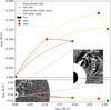 |
Fig. 1 PSP (in purple) and BepiColombo (in yellow) heliospheric locations in the XY plane (top) and in the YZ plane (bottom) of the Heliocentric Earth Ecliptic (HEE) reference frame. The solid line, the dash-dotted line, and the transparent dashed line stand for the trajectories, the Parker Spiral line, and the radial position of each spacecraft, respectively. Each trajectory begins (green points) on June 18, 2023, at 00:00 UTC and ends (red points) on June 20, 2023, at 00:00 UTC. Superimposed onto the bottom plot is a C2 and C3 LASCO coronograph, running-difference image of the Sun and near-Sun environment obtained from the SOHO spacecraft in June 18, 2023, around 04:45 UTC. |
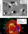 |
Fig. 2 (a) ADAPT-GONG magnetogram of June 18, 2023, at 00:00 UTC, in a Carrington reference frame. The white and black spots correspond, respectively, to positive and negative radial components of the magnetic field. The blue cross and light blue dot symbol and the red plus symbol and yellow star represent, respectively, the magnetic footpoints estimated with a PFSS model, of BepiColombo and PSP, respectively. The transparent yellow and pink circles mark the location of solar eruptions automatically detected by ER from the UV AIA imager at |


3 In situ observations: Spacecraft and method
3.1 Instruments and method
In this section, we leverage the positions of both spacecraft and their instruments to probe the SW parameters. At PSP, we used the fluxgate magnetometer (PSP-MAG) (Bale et al. 2016) and the Radio Frequency Spectrometer Low Frequency Receiver (RFS/LFR) (Pulupa et al. 2017), both part of the FIELDS suite, to measure the magnetic field and the electron density, respectively. The electron density was derived using the quasi-thermal noise technique (Moncuquet et al. 2020). Additionally, we used the Solar Probe Cup (SPC), a Faraday cup integrated into the Solar Wind Electron Alpha and Protons (SWEAP) instrument suite (Case et al. 2020), to estimate the SW velocity. We verified that the spacecraft’s orbital velocity was low compared to the radial one during the entire observation period, to avoid underestimating the SW speed due to PSP’s orbital motion close to the Sun. At BepiColombo, the same parameters were measured: the magnetic field with the fluxgate magnetometer on board the MPO spacecraft (MPO-MAG) (Glassmeier et al. 2010), the electron density with the Mercury Electron Analyzer (MEA) (Saito et al. 2021), and the SW velocity with the Planetary Ion Camera (PICAM), part of the Search for Exospheric Refilling and Emitted Natural Abundances (SERENA) suite (Orsini et al. 2021). PICAM is mounted on the side panel of BepiColombo’s MPO spacecraft, which adds some limitations for SW monitoring. Nevertheless, from the portion of the SW that falls into PICAM’s field of view, it is possible to estimate the SW speed.
To compare the observations from the two spacecraft, we performed a propagation of the magnetic field and plasma parameters from PSP to BepiColombo. Figure 4 was obtained using a SW velocity of  for the propagation. The value was taken from the bottom panel in Fig. 3, as it approximately corresponds to the speed measured before the onset of the perturbation at PSP. The electron density and magnetic field values propagated from PSP to BepiColombo were adjusted by multiplying their values by the square of the ratio of the spacecraft distances,
  Sun et al. (2022). Finally, the SW speed measured by PICAM was smoothed using a sliding average window of 3 hours to facilitate a comparison with the values extracted from SPC.
3.2 Observations from Parker Solar Probe
The top panel in Fig. 3 shows the magnetic field in the radial tangential normal (RTN) frame, where the black, blue, light blue, and red lines represent the magnitude, radial, tangential, and normal components, respectively. A low-pass filter with a cutoff frequency of  was applied to the magnetic field data, allowing us to focus on larger-scale structures. The middle panel displays the electron density, derived using the quasi-thermal noise technique from the FIELDS instrument (Moncuquet et al. 2020). Finally, the bottom panel shows the proton velocity measured by the SPC instrument (Case et al. 2020).
From the beginning of the time interval until June 18, 2023, at 09:30 UTC, the magnetic field is purely radial, indicating that PSP is observing the background SW. Between June 18, 2023, at 09:30 UTC and 21:00 UTC, while the SW remains mostly radial, more intense fluctuations are observed in the radial and tangential components of the magnetic field (with  decreasing as
  increases). Notably, the background SW exhibits a positive radial component, consistent with the PFSS model results shown in Fig. 2a. After this period, PSP no longer observes the background magnetic field and instead encounters a significant perturbation, possibly associated with the CMEs identified in LASCO C2 images in Fig. 1. This perturbation lasts approximately 27 hours, beginning on June 18, 2023, at 22:30 UTC and ending on June 20, 2023, at 01:30 UTC.
This is evident in each panel in Figure 3. First, we observe a dip in the magnetic field magnitude, where the components are predominantly normal and tangential, both strongly negative, while the radial component decreases to nearly zero. Around June 19, 2023, at 12:00 UTC, SW begins to recover its initial configuration, with the magnetic field becoming mostly radial again. During the last 5 hours of the perturbation, the magnetic field transitions to be primarily tangential. Unlike the earlier part of the perturbation, the normal component fluctuates around zero. Notably, the radial component of the magnetic field and the proton speed appear to be anticorrelated. Throughout the time interval, the SW speed remains very slow, starting at around  before the perturbation and decreasing further to
  afterward. Lastly, we observe four distinct density increases: the first three peaks reach approximately
  , while the final peak reaches
  and persists for several hours.
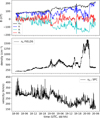 |
Fig. 3 Measurement of (top) the magnetic field in the RTN reference frame, (middle) electron density, and (bottom) the proton speed at PSP from June 18, 2023, at 00:00 to June 20, 2023, at 06:00. |
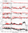 |
Fig. 4 Comparison of the magnetic field in the MSO frame, electron density, and SW speed: (a) |


3.3 Propagation at BepiColombo
As was previously mentioned, we performed a ballistic propagation of the plasma from PSP to BepiColombo to determine whether the perturbation was also detected at BepiColombo. Figure 4 compares the magnetic field in the Mercury Solar Orbital (MSO) frame, the electron density, and the SW velocity measured at both spacecraft. From panel (a) to (f), we show  , the electron density,
  , and the SW velocity,
  , respectively. The solid red and black lines are data extracted from BepiColombo and PSP sensors, respectively. PSP data are timeshifted to the corresponding location of BepiColombo. We excluded data recorded during MFB3 to focus solely on the SW plasma. The vertical dotted black lines delimit the time interval of MFB3.
The comparison reveals a good agreement between the densities observed at the two spacecraft, in terms of both magnitude and fluctuations, despite the uncertainties introduced by the ballistic propagation. Regarding the SW speed, the measurements from PICAM on board BepiColombo are generally higher than the ones from PSP. However, the velocity profiles exhibit a similar temporal evolution, with both reaching a minimum before increasing again. The higher background SW speed measured at BepiColombo compared to PSP is consistent with the acceleration of the slow SW, as has been demonstrated by Dakeyo et al. (2022). Finally, we compared the magnetic field measured with MPO-MAG on board BepiColombo with the propagated one of PSP-MAG. We applied the same procedure as MPOMAG for PSP-MAG to decrease the time resolution. As we scaled PSP-MAG data for the BepiColombo distance from the Sun, we compared only the variations between PSP-MAG and MPO-MAG data.
First, we observe that the  component of MPO-MAG is negative. In the MSO frame,
  corresponds to
  in the RTN frame. Therefore, this measurement is consistent with the PFSS model shown in Fig. 2 and supports the location of the background SW source at the surface of the Sun. We observe the perturbation seen in Fig. 3 at PSP between June 19, 2023, at 22:30 UTC and June 21, 2023, at 01:30 UTC, when comparing
  and
and  of MPO-MAG with the propagated PSP-MAG. The global shape of the perturbation is preserved in both
  and
and  . However, due to the longitude difference between the spacecraft and the real effect of propagation, the perturbation measured at BepiColombo is distorted compared to that at PSP. In
  , the perturbation is shorter at BepiColombo than at PSP, whereas in
  , they appear to last the same amount of time.
PSP-MAG measures a negative  for at least 6 hours, from June 19, 2023, at 18:00 until June 20, 2023, at 00:00 UTC. At BepiColombo, the same occurs for 5 hours, from June 19, 2023, at 16:30 until 21:50 UTC, despite a data gap due to MFB3. The time shift could be explained by the deformation during propagation. We observe that
  and
and  before and after MFB3. However, we see that the magnetic field magnitude is twice as high at the outbound side of MFB3 compared to the inbound side. In terms of intensity, the same is observed for
  , which becomes twice as negative after the MFB3 exit. All these factors tend to confirm that the IMF orientation was southward for several hours at Mercury, as it was at PSP, at the beginning of the perturbation.
4 Discussion and conclusions
In this study, we use the PSP-Sun-Mercury conjunction to characterize the SW properties during MFB3. Based on the PFSS model, we found that PSP and BepiColombo were connected to the same magnetic footpoints. Magnetic field measurements from both spacecraft were consistent with the model, as both radial components were positive. PSP data revealed a slow perturbation passing through it. By monitoring solar activity using SDO/AIA, SolO/EUI, and SOHO LASCO coronagraphs, we suggest that PSP was not directly impacted by a slow CME but rather perturbed by an encounter far from the core. At BepiColombo, the in situ measurements are consistent with such a hypothesis as no clear shock signature is observed in the magnetic field and SW speed data. This suggests instead a compressed region along the flank of the outflowing transient CME. The regions where the CMEs originated and the locations of the magnetic footpoints of the background SW are associated with coronal loops. At the beginning of the perturbation, PSP observed a significant change in the IMF orientation.  abruptly decreased, indicating that the magnetic field was mostly perpendicular to SW propagation, while
  remained negative for several hours. During the perturbation, the SW speed decreased, and the density fluctuated, increasing multiple times. By propagating the SW ballistically to BepiColombo, we observed a consistency with the fluctuations and the order of magnitude of the measured density. The magnetic field fluctuations observed with MPO-MAG are also in agreement with the ones seen at PSP. We conclude that the
  component (in the MSO frame) remained negative throughout MFB3, with the magnitude of
  increasing during the flyby.
A strong southward IMF is a key feature of the SW interaction with the Hermean magnetosphere, as has been experimentally observed (Leyser et al. 2017; Jasinski et al. 2017; Chen et al. 2019). On the dayside, magnetic reconnection is continuously driven, regardless of the IMF orientation. However, a southward IMF reconnects around the subsolar point. The newly created open-field lines fill the polar caps, causing the boundaries between the open and closed field lines to get closer from the magnetic equator. Moreover, the subsolar standoff distance of the MP moves closer to the surface (Varela et al. 2015). Magnetic energy is stored in the lobes of the magnetotail, and this energy is converted into kinetic energy when plasma flows planetward or tailward, following magnetic reconnection in the plasma sheet. Particles can be accelerated from a few kiloelectronvolts to hundreds of kilo-electronvolts through Betatron or Fermi acceleration as they reach the inner magnetosphere. Finally, several dawn-dusk asymmetries arise in the magnetotail, such as dipolarizations, reconnection fronts, and energetic electron injections, which tend to appear more frequently on the dawnside. Another important dawn-dusk asymmetry is observed at the surface of Mercury. Lindsay et al. (2016) show that regions near the boundary between open and closed field lines are the source of X-ray fluorescence. Dewey et al. (2017) conducted test particle tracing of energetic electrons, showing that they should precipitate in the same areas. Different simulations predict that energetic particles precipitate in the night-dawn sector.
Recently, the interaction of the SW with Mercury’s minimagnetosphere and surface has been studied numerically using full kinetic 3D simulations (Lavorenti et al. 2022, 2023). These studies focus on the influence of IMF orientation when SW electrons interact with the Hermean magnetosphere at the electron kinetic scale. The authors show that when the IMF is oriented southward, magnetotail reconnection can accelerate electrons up to tens of kilo-electronvolts, producing a dawn-dusk asymmetry on the nightside, where the electron temperature and density are higher. This result is also confirmed by the simulations of Chen et al. (2019), a global MHD simulation with an embedded particle-in-cell model. Their simulations show a higher plasma density and electron pressure on the dawnside, close to the planet. The simulations by Lavorenti et al. (2023) also explain how changes in IMF orientation affect the areas where electrons precipitate on the surface, correlating with the emission of X-ray fluorescence induced by electron impacts.
Compared to the first and second MFBs (MFB1 and MFB2), the magnetosphere was most compressed during MFB3 (Rojo et al. 2024). The dynamic pressure of the SW was rather low, about 32 nPa , due to a low SW speed, even the high density, ranging from 100 to 300 cm−3, compared to the average density of 50 cm−3 typically observed around 0.3 AU (Sun et al. 2022). The authors also observed dawn-dusk asymmetries, with high electron energy fluxes measured by MEA in the nightside dawn sector. Aizawa et al. (2023) illustrate how multiple high-energy electron bursts were related to substorms during MFB1 of BepiColombo. They show, through test particle tracing, that these electrons could precipitate in regions where X-ray fluorescence is emitted. During the second MFB (MFB2) by BepiColombo, sporadic bursts of high-energy electron flux were observed only in the nightside dawn sector (Rojo et al. 2024). This is consistent with the findings of Lavorenti et al. (2022) and Chen et al. (2019), which show that accelerated electrons drift dawnward, close to the planet. However, during MFB3, MEA measured electrons with energies of a few tens of kilo-electronvolts, starting in the pre-midnight sector and continuing almost continuously until the outbound MP, for a duration of just over 15 minutes. During the same time interval, high-energy fluxes of ions were also measured by the Mercury Ion Analyzer and the Mass Spectrum Analyzer (Hadid et al. 2024; Harada et al. 2024) on board BepiColombo. Hadid et al. (2024) identify this region as the plasma sheet horn, a high-latitude region of the plasma sheet. After magnetotail reconnection, the hot plasma flow decelerates as it interacts more strongly with the dipole field. The plasma then separates and flows toward higher latitudes, at the openclosed field line boundary (Glass et al. 2022). Recently, Shao et al. (2023) demonstrated, based on the work of Sun et al. (2015), that successive magnetotail reconnections with multiple energy-release processes occur at Mercury for several minutes.
By studying the SW conditions during MFB3, we show that Mercury was not directly impacted by CMEs and suggest that it was rather impacted by a compressed region along the flank of an outflowing transient CME. The dynamic pressure of the SW was low, yet it carried a strong southward IMF. This suggests that the IMF orientation was the primary driver of continuous magnetotail reconnection, leading to the energization of both electrons and ions observed on the dawn-side nightside during MFB3. This observation could have significant implications for space weathering on Mercury’s nightside. The SW plasma parameters and IMF orientation should be used to further constrain simulations of this specific flyby or, more broadly, magnetotail reconnection at Mercury. Moreover, to test this hypothesis, the high-energy particle data from the SIXS (Solar Intensity X-ray and Particles Spectrometer) and HEP-e (High Energy Particles electron) instruments should be analyzed.
Data availability
The BepiColombo density, SW speed and magnetic field data displayed here are available for download at https://zenodo.org/uploads/14620890. The PSP measurement data used here are publicly available at https://cdaweb.gsfc.nasa.gov/. The radial velocity profile from the iso-poly model of J.B. Dakeyo, was calculated using the S.T. Badman scripts, available at https://github.com/STBadman/ParkerSolarWind?tab=readme-ov-file The movie associated to Fig. 2 is available at https://www.aanda.org
Movie
Movie associated to Fig 2 Access Supplementary Material
Acknowledgments
French co-authors acknowledge the support of Centre National d’Etudes Spatiales (CNES, France) to the BepiColombo and Parker Solar Probe missions. BepiColombo is a joint space mission between the European Space Agency (ESA) and the Japan Aerospace Exploration Agency (JAXA). MPPE is funded by JAXA, CNES, the Centre National de la Recherche scientifique (CNRS, France), the Italian Space Agency (ASI), and the Swedish National Space Agency (SNSA). SERENA management are funded by ASI, the Italian National Institute of Astrophysics (INAF), and the ground-based activities by ESA (EXPRO contract). SERENA/PICAM is funded by the Austrian Space Applications Program of the Austrian Research Promotion Agency (FFG), ESA’s Program de Développement d’Expériences (PRODEX) and CNES. The FIELDS experiment on the Parker Solar Probe spacecraft was designed and developed under NASA contract NNN06AA01C. At the start of this work M.R. was funded by the European Union’s Horizon 2020 program under grant agreement No. 871149 for Europlanet 2024 RI. DH was supported by the German Ministerium für Wirtschaft und Energie and the German Zentrum für Luft-und Raumfahrt under contract 50 QW1501. L.R.-G. acknowledges support through the European Space Agency (ESA) research fellowship programme. This paper uses data from the CACTus CME catalog, generated and maintained by the SIDC at the Royal Observatory of Belgium.
References
- Aizawa, S., Harada, Y., André, N., et al. 2023, Nat. Commun., 14, 4019 [NASA ADS] [CrossRef] [Google Scholar]
- Aizawa, S., Rojo, M., André, N., et al. 2024, Nat. Commun., submitted [Google Scholar]
- Badman, S. T., Bale, S. D., Oliveros, J. C. M., et al. 2020, ApJS, 246, 23 [Google Scholar]
- Baker, D., Simpson, J., & Eraker, J. 1986, J. Geophys. Res.: Space Phys., 91, 8742 [Google Scholar]
- Bale, S., Goetz, K., Harvey, P., et al. 2016, Space Sci. Rev., 204, 49 [Google Scholar]
- Brueckner, G. E., Howard, R. A., Koomen, M. J., et al. 1995, Sol. Phys., 162, 357 [NASA ADS] [CrossRef] [Google Scholar]
- Case, A. W., Kasper, J. C., Stevens, M. L., et al. 2020, ApJS, 246, 43 [Google Scholar]
- Chen, Y., Tóth, G., Jia, X., et al. 2019, J. Geophys. Res.: Space Phys., 124, 8954 [Google Scholar]
- Christon, S. 1987, Icarus, 71, 448 [NASA ADS] [CrossRef] [Google Scholar]
- Dakeyo, J.-B., Maksimovic, M., Démoulin, P., Halekas, J., & Stevens, M. L. 2022, ApJ, 940, 130 [NASA ADS] [CrossRef] [Google Scholar]
- Dakeyo, J.-B., Badman, S., Rouillard, A., et al. 2024, A&A, 686, A12 [NASA ADS] [CrossRef] [EDP Sciences] [Google Scholar]
- Dewey, R. M., Raines, J. M., Sun, W., Slavin, J. A., & Poh, G. 2017, Geophys. Res. Lett., 45, 10 [Google Scholar]
- Fatemi, S., Poppe, A. R., & Barabash, S. 2020, J. Geophys. Res. Space Phys., 125, e2019JA027706 [Google Scholar]
- Glass, A., Raines, J., Jia, X., et al. 2022, J. Geophys. Res.: Space Phys., 127, e2022JA030969 [Google Scholar]
- Glassmeier, K.-H., Auster, H.-U., Heyner, D., et al. 2010, Planet. Space Sci., 58, 287 [NASA ADS] [CrossRef] [Google Scholar]
- Hadid, L. Z., Delcourt, D., Harada, Y., et al. 2024, Commun. Phys., 7, 316 [Google Scholar]
- Harada, Y., Saito, Y., Hadid, L. Z., et al. 2024, J. Geophys. Res.: Space Phys., 129, e2024JA032751 [Google Scholar]
- Hickmann, K. S., Godinez, H. C., Henney, C. J., & Arge, C. N. 2015, Sol. Phys., 290, 1105 [NASA ADS] [CrossRef] [Google Scholar]
- Hill, F. 2018, Space Weather, 16, 1488 [NASA ADS] [CrossRef] [Google Scholar]
- Hurlburt, N. 2015, J. Space Weather Space Clim., 5 [Google Scholar]
- Imber, S. M., & Slavin, J. 2017, J. Geophys. Res.: Space Phys., 122, 11 [Google Scholar]
- Jasinski, J. M., Slavin, J. A., Raines, J. M., & DiBraccio, G. A. 2017, J. Geophys. Res.: Space Phys., 122, 12 [Google Scholar]
- Lapenta, G., Schriver, D., Walker, R. J., et al. 2022, J. Geophys. Res.: Space Phys., 127, e2021JA030241 [Google Scholar]
- Lavorenti, F., Henri, P., Califano, F., et al. 2022, A&A, 664, A133 [NASA ADS] [CrossRef] [EDP Sciences] [Google Scholar]
- Lavorenti, F., Henri, P., Califano, F., et al. 2023, A&A, 674, A153 [NASA ADS] [CrossRef] [EDP Sciences] [Google Scholar]
- Lavraud, B., Fargette, N., Réville, V., et al. 2020, ApJ, 894, L19 [Google Scholar]
- Leyser, R. P., Imber, S. M., Milan, S. E., & Slavin, J. A. 2017, Geophys. Res. Lett., 44, 10 [NASA ADS] [CrossRef] [Google Scholar]
- Lindsay, S., James, M., Bunce, E., et al. 2016, Planet. Space Sci., 125, 72 [NASA ADS] [CrossRef] [Google Scholar]
- Markidis, S., Lapenta, G., et al. 2010, Math. Comput. Simul., 80, 1509 [Google Scholar]
- Moncuquet, M., Meyer-Vernet, N., Issautier, K., et al. 2020, ApJS, 246, 44 [Google Scholar]
- Müller, J., Simon, S., Motschmann, U., et al. 2011, Comput. Phys. Commun., 182, 946 [CrossRef] [Google Scholar]
- Murray, S. A., Guerra, J. A., Zucca, P., et al. 2018, Sol. Phys., 293, 1 [NASA ADS] [CrossRef] [Google Scholar]
- Ness, N., Behannon, K., Lepping, R., Whang, Y., & Schatten, K. 1974, Science, 185, 151 [NASA ADS] [CrossRef] [Google Scholar]
- Ogilvie, K., Scudder, J., Hartle, R., et al. 1974, Science, 185, 145 [NASA ADS] [CrossRef] [Google Scholar]
- Orsini, S., Livi, S., Lichtenegger, H., et al. 2021, Space Sci. Rev., 217, 1 [NASA ADS] [CrossRef] [Google Scholar]
- Persson, M., Aizawa, S., André, N., et al. 2022, Nat. Commun., 13, 7743 [NASA ADS] [CrossRef] [Google Scholar]
- Poh, G., Slavin, J. A., Jia, X., et al. 2017, J. Geophys. Res.: Space Phys., 122, 8419 [Google Scholar]
- Pulupa, M., Bale, S., Bonnell, J., et al. 2017, J. Geophys. Res.: Space Phys., 122, 2836 [NASA ADS] [CrossRef] [Google Scholar]
- Robbrecht, E., & Berghmans, D. 2004, A&A, 425, 1097 [NASA ADS] [CrossRef] [EDP Sciences] [Google Scholar]
- Rojo, M., Persson, M., Sauvaud, J.-A., et al. 2024, A&A, 683, A99 [NASA ADS] [CrossRef] [EDP Sciences] [Google Scholar]
- Rojo, M., André, N., Aizawa, S., et al. 2024, A&A, 687, A243 [NASA ADS] [CrossRef] [EDP Sciences] [Google Scholar]
- Rouillard, A. P., Pinto, R. F., Vourlidas, A., et al. 2020, A&A, 642, A2 [NASA ADS] [CrossRef] [EDP Sciences] [Google Scholar]
- Saito, Y., Delcourt, D., Hirahara, M., et al. 2021, Space Sci. Rev., 217, 1 [NASA ADS] [CrossRef] [Google Scholar]
- Shao, P., Ma, Y., & Zeng, G. 2023, ApJ, 953, 110 [Google Scholar]
- Slavin, J., Owen, J., Connerney, J., & Christon, S. 1997, Planet. Space Sci., 45, 133 [Google Scholar]
- Solomon, S. C., McNutt Jr, R. L., Gold, R. E., et al. 2001, Planet. Space Sci., 49, 1445 [NASA ADS] [CrossRef] [Google Scholar]
- Sun, W.-J., Slavin, J. A., Fu, S., et al. 2015, Geophys. Res. Lett., 42, 3692 [Google Scholar]
- Sun, W., Dewey, R. M., Aizawa, S., et al. 2022, Sci. China Earth Sci., 1 [Google Scholar]
- Varela, J., Pantellini, F., & Moncuquet, M. 2015, Planet. Space Sci., 119, 264 [NASA ADS] [CrossRef] [Google Scholar]
All Figures
|
Fig. 1 PSP (in purple) and BepiColombo (in yellow) heliospheric locations in the XY plane (top) and in the YZ plane (bottom) of the Heliocentric Earth Ecliptic (HEE) reference frame. The solid line, the dash-dotted line, and the transparent dashed line stand for the trajectories, the Parker Spiral line, and the radial position of each spacecraft, respectively. Each trajectory begins (green points) on June 18, 2023, at 00:00 UTC and ends (red points) on June 20, 2023, at 00:00 UTC. Superimposed onto the bottom plot is a C2 and C3 LASCO coronograph, running-difference image of the Sun and near-Sun environment obtained from the SOHO spacecraft in June 18, 2023, around 04:45 UTC. |
| In the text | |
|
Fig. 2 (a) ADAPT-GONG magnetogram of June 18, 2023, at 00:00 UTC, in a Carrington reference frame. The white and black spots correspond, respectively, to positive and negative radial components of the magnetic field. The blue cross and light blue dot symbol and the red plus symbol and yellow star represent, respectively, the magnetic footpoints estimated with a PFSS model, of BepiColombo and PSP, respectively. The transparent yellow and pink circles mark the location of solar eruptions automatically detected by ER from the UV AIA imager at |
| In the text | |
|
Fig. 3 Measurement of (top) the magnetic field in the RTN reference frame, (middle) electron density, and (bottom) the proton speed at PSP from June 18, 2023, at 00:00 to June 20, 2023, at 06:00. |
| In the text | |
|
Fig. 4 Comparison of the magnetic field in the MSO frame, electron density, and SW speed: (a) |
| In the text | |
Current usage metrics show cumulative count of Article Views (full-text article views including HTML views, PDF and ePub downloads, according to the available data) and Abstracts Views on Vision4Press platform.
Data correspond to usage on the plateform after 2015. The current usage metrics is available 48-96 hours after online publication and is updated daily on week days.
Initial download of the metrics may take a while.