| Issue |
A&A
Volume 692, December 2024
|
|
|---|---|---|
| Article Number | A136 | |
| Number of page(s) | 10 | |
| Section | Planets, planetary systems, and small bodies | |
| DOI | https://doi.org/10.1051/0004-6361/202451926 | |
| Published online | 06 December 2024 | |
Global magnetic field properties in the solar wind interaction of Mercury from MESSENGER measurements
1
Key Laboratory of Earth and Planetary Physics, Institute of Geology and Geophysics, Chinese Academy of Sciences,
Beijing
100029,
China
2
College of Earth and Planetary Sciences, University of Chinese Academy of Sciences,
Beijing
100049,
China
★ Corresponding author; j.zhong@mail.iggcas.ac.cn
Received:
19
August
2024
Accepted:
1
November
2024
Context. The space environment of Mercury is shaped by its proximity to the Sun and by the relatively weak planetary magnetic field, presenting a unique regime of plasmas and shock conditions.
Aims. We present the global magnetic properties in Mercury’s space environment based on more than 4 years of MESSENGER Magnetometer data.
Methods. We used 20 Hz magnetic field data to examine the magnetic strength, the field configurations, and the fluctuations. We considered both compressional and transverse modes, with frequencies from 5 mHz to 10 Hz, which cover typical ultra-low frequency waves at Mercury. We identified regions of the solar wind, the magnetosheath, and the magnetosphere during over 4000 MESSENGER orbits. The solar wind and magnetosheath data were analysed in the solar wind interplanetary magnetic field (IMF) coordinate system, and the magnetosphere data were analysed in the aberrated Mercury solar magnetospheric coordinate system. Each data point was relocated into normalised space using averaged magnetopause and bow-shock models. The magnetic environments for a quasi-parallel and quasi-perpendicular IMF were compared.
Results. Under the typical Parker-spiral IMF, the magnetic environment of Mercury features strong fluctuations that are dominated by the transverse mode and stem from interactions at the bow shock and the magnetopause. When they are subjected to a quasi-perpendicular IMF, the magnetic fluctuations diminish, and the magnetic field strength becomes highly compressed throughout the bow shock, magnetosheath, and magnetosphere. Unlike Earth, Mercury exhibits weaker dawn-dusk asymmetries in magnetic field strength and lacks substantial magnetosheath-generated sources of magnetic fluctuations. The magnetic field draping pattern associated with the IMF cone angle at Mercury also differs from that at Earth.
Conclusions. Our comparative analysis highlights the critical role of the solar wind Mach number, the radial IMF component, and the system scale size in shaping planetary space environments.
Key words: Sun: magnetic fields / solar-terrestrial relations / planets and satellites: magnetic fields / planets and satellites: terrestrial planets
© The Authors 2024
 Open Access article, published by EDP Sciences, under the terms of the Creative Commons Attribution License (https://creativecommons.org/licenses/by/4.0), which permits unrestricted use, distribution, and reproduction in any medium, provided the original work is properly cited.
This article is published in open access under the Subscribe to Open model. Subscribe to A&A to support open access publication.
1 Introduction
The solar wind interacts with a magnetised planet to form a magnetic cavity called the magnetosphere, in which the plasma behaviour is controlled by the planetary magnetic field. Upstream, a bow shock slows, compresses, heats, and deflects the solar wind flow around the magnetosphere, creating a boundary called the magnetopause. The magnetic and plasma properties of the interface between the bow shock and the magnetopause, namely, the magnetosheath, are dictated by the physical processes within the shock. Large differences in the upstream solar wind conditions and internal planetary field properties create unique space environments for each planet.
Among terrestrial planets, only Mercury possesses an Earth-like global magnetic field, and consequently, a magnetosphere. As the innermost planet, Mercury experiences the most dynamic heliospheric space environment. The solar wind exposes Mercury to a much higher ram pressure than at Earth, it is about ten times greater, and the interplanetary magnetic field (IMF) is significantly stronger with ~30 nT, in contrast to ~5 nT at Earth (Burlaga 2001). Additionally, the IMF at Mercury primarily points radially toward or away from the Sun, which means that its bow-shock normal is more likely to be quasi-parallel to the solar wind flow than at other planets (James et al. 2017). Furthermore, the lower Alfvén Mach number (the ratio of the plasma speed to the Alfvén speed) results in the weakest planetary bow shock in the Solar System (Masters et al. 2013). All of these phenomena at Mercury recall the conditions at the close-in exoplanets around M dwarfs (Dong et al. 2018).
Mercury is the least explored terrestrial planet. Our insights mainly arise from three flybys by the Mariner 10 spacecraft in 1974 and 1975 (Ness et al. 1975) and the MESSENGER spacecraft, which orbited around the planet from 2011 to 2015 (Solomon et al. 2018). The magnetic field of Mercury, a spinaligned dipole offset by 0.2 RM to the north, has a dipole moment of 190 nT ![$\[R_{M}^{3}\]$](/articles/aa/full_html/2024/12/aa51926-24/aa51926-24-eq1.png) , approximately three orders of magnitude weaker than that of Earth (Anderson et al. 2011, 2012; Exner et al. 2024). This creates a compact, highly dynamic magnetosphere that reaches only 5% of the size of the terrestrial magnetosphere (Winslow et al. 2013; Zhong et al. 2015a,b). The small-scale system responds rapidly to variations in the solar wind. The characteristic timescales for convection and wave transits through the magnetosphere are only 1–2 min, which is nearly two orders of magnitude shorter than the timescale at Earth (Slavin et al. 2021). Lacking an atmosphere or ionosphere, Mercury’s space environment is better described as a solar wind–magnetosphere–exosphere–surface interaction rather than the solar wind–magnetosphere–ionosphere coupled system, which exists at other magnetised planets in the Solar System (Orsini et al. 2007).
, approximately three orders of magnitude weaker than that of Earth (Anderson et al. 2011, 2012; Exner et al. 2024). This creates a compact, highly dynamic magnetosphere that reaches only 5% of the size of the terrestrial magnetosphere (Winslow et al. 2013; Zhong et al. 2015a,b). The small-scale system responds rapidly to variations in the solar wind. The characteristic timescales for convection and wave transits through the magnetosphere are only 1–2 min, which is nearly two orders of magnitude shorter than the timescale at Earth (Slavin et al. 2021). Lacking an atmosphere or ionosphere, Mercury’s space environment is better described as a solar wind–magnetosphere–exosphere–surface interaction rather than the solar wind–magnetosphere–ionosphere coupled system, which exists at other magnetised planets in the Solar System (Orsini et al. 2007).
Magnetic activities are prevalent in the coupled small and compressed system, including foreshock waves and standing whistler waves from the bow shock (Le et al. 2013; Romanelli & DiBraccio 2021; Wang et al. 2023), ion cyclotron waves in the solar wind and magnetosheath (Sundberg et al. 2015; Schmid et al. 2021), Kelvin-Helmholtz instability/waves at the magnetopause (Sundberg et al. 2012a; Gershman et al. 2015), and various ultra-low frequency (ULF) waves in the magnetosphere (Boardsen et al. 2012; Liljeblad & Karlsson 2017; James et al. 2019). High-efficiency reconnection at the dayside magnetopause and nightside current sheet drives sudden magnetic field disturbances in the magnetosphere, such as rapid successions of flux transfer events (FTEs) at the magnetopause (Slavin et al. 2012; Sun et al. 2020; Zhong et al. 2020c), magnetotail flux ropes and plasmoids (DiBraccio et al. 2015; Smith et al. 2017; Zhong et al. 2019, 2020a), dipolarisations and reconnection fronts (Sundberg et al. 2012b; Sun et al. 2016; Zhong et al. 2018; Dewey et al. 2020), and potential substorm activities (Sun et al. 2015; Imber & Slavin 2017; Poh et al. 2017; Dewey et al. 2020).
To understand the global magnetic and plasma environment in the interaction between the solar wind and Mercury, a large number of three-dimensional global simulations were performed, including magnetohydrodynamics (MHD; Dong et al. 2019; Ip & Kopp 2002; Griton et al. 2023; Jia et al. 2015, 2019; Zhong et al. 2024), hybrid (Aizawa et al. 2021; Lu et al. 2022; Kallio et al. 2022; Paral et al. 2010; Vernisse et al. 2017; Trávníček et al. 2010; Exner et al. 2018, 2020), and particle-in-cell (Lavorenti et al. 2022; Ballerini, Giulio et al. 2024) models. These models focus on specific phenomena under particular solar wind and IMF conditions and thus revealed a high variability in the solar wind interaction of Mercury.
We present the global magnetic field properties around Mercury, including the solar wind, the magnetosheath, and the magnetosphere, using over 4 years of MESSENGER orbital magnetic field observations. We compare the average magnetic properties under quasi-parallel and quasi-perpendicular IMF conditions and discuss fundamental space-science topics, such as magnetic field draping, magnetic fluctuation sources, and the dawn-dusk asymmetry, in comparison with those of Earth.
2 Methods
2.1 Data and coordinates
MESSENGER was the first spacecraft to orbit Mercury and spent more than 4 years (March 18, 2011, to April 30, 2015) orbiting the planet and observing its magnetic environment (Solomon et al. 2007). In this study, we use the magnetic field data from the magnetometer instrument (MAG) with a 20 Hz sampling rate (Anderson et al. 2007). The magnetic fluctuations (dB) are defined as the square root of the standard deviation of three magnetic components, ![$\[\mathrm{dB}=\sqrt{\frac{1}{\mathrm{~N}} {\sum}_{i=1}^{\mathrm{N}}\left[\left(B_{x_{i}}-\left\langle B_{x}\right\rangle\right)^{2}+\left(B_{y_{i}}-\left\langle B_{y}\right\rangle\right)^{2}+\left(B_{z_{i}}-\left\langle B_{z}\right\rangle\right)^{2}\right]}\]$](/articles/aa/full_html/2024/12/aa51926-24/aa51926-24-eq2.png) . Both compressional and transverse fluctuation components were considered and computed using the formula
. Both compressional and transverse fluctuation components were considered and computed using the formula ![$\[\mathrm{dB}_{\mathrm{c}}=\left[\frac{1}{\mathrm{~N}} {\sum}_{i=1}^{\mathrm{N}}\left(\left|B_{i}\right|-\langle | B| \rangle\right)^{2}\right]^{\frac{1}{2}}\]$](/articles/aa/full_html/2024/12/aa51926-24/aa51926-24-eq3.png) for the compressional component and
for the compressional component and ![$\[\mathrm{dB}_{\mathrm{t}}=\left(\mathrm{dB}^{2}-\mathrm{dB}_{\mathrm{c}}^{2}\right)^{\frac{1}{2}}\]$](/articles/aa/full_html/2024/12/aa51926-24/aa51926-24-eq4.png) for the transverse component. A 100 s window of MESSENGER measurements was used to calculate a data point every second. This approach allowed us to resolve frequencies ranging from 5 mHz to 10 Hz, which cover the typical ULF wave frequencies at Mercury.
for the transverse component. A 100 s window of MESSENGER measurements was used to calculate a data point every second. This approach allowed us to resolve frequencies ranging from 5 mHz to 10 Hz, which cover the typical ULF wave frequencies at Mercury.
The basic coordinate systems we used are the aberrated Mercury solar magnetospheric (MSM) coordinate system and solar wind interplanetary magnetic field (SWI) coordinate system. The MSM coordinate system is centred on the internal dipole of Mercury (offset to 0.2 RM north of the planet centre), with the x-axis pointing from the dipole centre towards the Sun, the z-axis pointing northward and aligned with the planetary spin axis, and the y-axis completing the right-handed systems (Anderson et al. 2011). The choice of the 0.2 RM northward dipole offset for the magnetic field of Mercury fits the MESSENGER observations best, which is supported by a comparative analysis of planetary magnetic field models (Exner et al. 2024). We rotated the x – and y-axes to account for the orbital motion of Mercury with respect to an average radial solar wind velocity of 400 km s−1. This produced an x-axis opposite to the solar wind flow in the Mercury frame.
The SWI coordinate system (Zhang et al. 2019) was adopted to examine the asymmetries related to the orientation of the IMF. This system depends on the IMF orientation and on the velocity of the solar wind. Here, the x-axis is the same as in aberrated MSM coordinates. The y-axis is defined along the magnetic field in the YZ plane, and the z-axis completes the right-hand coordinate system through Z = X × Y. For IMF BX < 0, the signs of the observed magnetic field are reversed; therefore, the IMF always points in the +X and −Y direction, and the parallel bow shock is thus always located on the −Y section (dawnside) and the perpendicular shock is on the +Y section (duskside). On a statistical basis, this prevents the overlap of magnetic properties that were transmitted under different shock configurations. The resulting magnetosheath closely resembles the configuration under nominal Parker-spiral IMF conditions. However, under an ortho-Parker spiral IMF, the dawn-dusk configuration is opposite to the MSM frame (Dimmock et al. 2014, 2017).
2.2 Identification of boundary positions
The bow shock and magnetopause crossings can be identified by abrupt changes in the magnetic field strength/direction, and they are assisted by a sharp boundary in the heated ion flux spectrogram between different regions (Zhong et al. 2015a, 2020b). An example of a MESSENGER orbital observation of the magnetic properties around Mercury is shown in Fig. 1. MESSENGER travelled from the solar wind into the magnetosheath at a southern high latitude, sequentially crossing the magnetosphere, moving out of the low-latitude magnetosheath, and finally returning to the solar wind (Figs. 1e and 1f). Evidently, the magnetic field is compressed and changes its direction across the bow shock from the solar wind to the magnetosheath and across the magnetopause from the magnetosheath to magnetosphere. The magnetic fluctuations are significantly enhanced upon crossing these boundaries. Particularly, in the downstream of the dayside bow shock, the amplitude of the normalised magnetosheath field fluctuations can approach one. Moreover, the magnetic fluctuations exhibit a strong anisotropy, predominantly in the transversal components. The magnetosphere is characterised by the strongest magnetic field amplitude and the lowest plasma density, and the ion flux spectrogram is nearly empty in the tail and more energetic in the dayside, which is different from the magnetosheath. MESSENGER was typically unable to measure the solar wind flow because of constraints related to the placement of the plasma instrument and spacecraft orientation.
Using the criteria from Zhong et al. (2015a, 2020b), we updated the list of the MESSENGER’s bow shock and magnetopause crossings to cover the entire orbital duration. A total of 8086 inbound and outbound passes were identified through visual inspection.
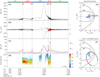 |
Fig. 1 Example of a MESSENGER orbital observation of the magnetic properties around Mercury. (a, b) Magnetic field magnitude and its three components in the aberrated MSM coordinates. (c) Magnetic fluctuation and its compressional/transversal components. (d) Spectrogram of the ion differential energy flux (cm−2 sr−1 s−1 keV−1). The horizontal green, red, and blue bars label the solar wind (SW), magnetosheath (MSH), and magnetosphere (MSP) regions, respectively. (e) and (f) MESSENGER orbit projected onto the equatorial and noon-midnight planes relative to the Mercury surface (circle) and the average magnetopause (MP) and bow shock (BS) from the model (Zhong et al. 2015a). |
2.3 Determination of the upstream IMF conditions
To determine the upstream IMF conditions, we used the average magnetic field measured over 15 min just upstream of the outer-most bow-shock crossings because there was no upstream IMF monitor. We considered the effect of the IMF cone angle, defined as θCA = cos−1 (Bx/|B|), which approximates the angle between the IMF and the opposite solar wind velocity vectors.
Figure 2a shows a histogram of IMF cone angles for all bow-shock passes. The two peaks correspond to the most common Parker-spiral IMF orientations at 30° and 150°, which is consistent with previous IMF statistics (Chang et al. 2019; He et al. 2017; James et al. 2017). Moreover, a bimodal distribution of BY was observed. The observations are divided into two cone-angle ranges: more parallel (|90° − θCA| > 45°), and more perpendicular (|90° − θCA| < 45°) to the solar wind direction. The former quasi-parallel case includes instances of the common Parker-spiral IMF and encompasses larger orbit events. The events of the latter quasi-perpendicular case are roughly half as frequent.
Figure 2b displays the distributions of the IMF strength. A comparison of the quasi-parallel and quasi-perpendicular IMF datasets reveals that the IMF strength is statistically lower under quasi-perpendicular conditions.
2.4 Spatial superposition analysis
Due to the variable positions of the bow shock and the magnetopause during different orbits, we relocated each data point to a normalised space using an averaged magnetopause and bowshock models. The bow shock was modelled by a conic section with a focus along the x-axis at X = X0 (Slavin et al. 2009; Winslow et al. 2013): ![$\[r_{B S}=\sqrt{\left(X-X_{0}\right)^{2}+Y^{2}+Z^{2}}=\frac{L}{1+\varepsilon \cos \theta}\]$](/articles/aa/full_html/2024/12/aa51926-24/aa51926-24-eq5.png) . Fitting our bow-shock crossing dataset resulted in X0 = 0.5 RM, L = 2.88 RM, and ϵ = 1.02, and the extrapolated bow-shock subsolar standoff distance is 1.9 RM. The magnetopause distance (rM P) was calculated using the magnetopause model from Shue et al. (1997):
. Fitting our bow-shock crossing dataset resulted in X0 = 0.5 RM, L = 2.88 RM, and ϵ = 1.02, and the extrapolated bow-shock subsolar standoff distance is 1.9 RM. The magnetopause distance (rM P) was calculated using the magnetopause model from Shue et al. (1997): ![$\[r_{M P}=r_{0}\left(\frac{2}{1+\cos \theta}\right)^{\alpha}\]$](/articles/aa/full_html/2024/12/aa51926-24/aa51926-24-eq6.png) . The fitting of our magnetopause crossing dataset resulted in a subsolar standoff distance r0 = 1.45 RM and in a flaring parameter α = 0.47. The value of the parameter α reflects the magnetopause shape, determining whether the tail is closed (<0.5), asymptotes to a finite tail radius (=0.5), or expands with increasing distance from Mercury (>0.5).
. The fitting of our magnetopause crossing dataset resulted in a subsolar standoff distance r0 = 1.45 RM and in a flaring parameter α = 0.47. The value of the parameter α reflects the magnetopause shape, determining whether the tail is closed (<0.5), asymptotes to a finite tail radius (=0.5), or expands with increasing distance from Mercury (>0.5).
To normalise the magnetosheath data, we used the fractional distance F = (r − rM P)/(rBS + rM P) between the bow shock and magnetopause, known as the magnetosheath-interplanetary medium reference frame (Verigin et al. 2006). Here, rM P and rBS are the radial distances to the magnetopause and bow shock along the spacecraft position r, respectively. The range of F spans from zero (magnetopause) to one (bow shock). This approach is best suited for a dayside analysis. For the nightside, we used the projected distance in the Y–Z plane instead of the radial distance.
Solar wind data were normalised by adjusting the radial distance, r = robs − rBS,obs + rBS,mod, where robs, rBS,obs, and rBS,mod are the radial distances of the observed data, the observed bow shock, and the modelled bow shock, respectively. For magnetosphere observations, we only considered data points with radial distances smaller than those in the model.
The magnetic field parameters within the solar wind and magnetosheath were normalised by the mean IMF magnitude for each crossing. To capture the variations in the magnetospheric field under different external conditions, the magnetospheric field was normalised by a constant value of 25 nT, which is approximately equal to the average IMF magnitude. Subsequently, all obtained values were binned into a grid, and the mean of the data points within each bin was used to construct the bin value.
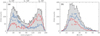 |
Fig. 2 Distribution of 15-minute averaged IMF cone angle (a) and intensity (b) upstream of the bow shock during the whole MESSENGER mission. The overall histogram of the cone angle is separated into two histograms according to the sign of BY (blue: negative; red: positive), and the magnetic field intensity is separated into two histograms according to the cone angle (blue: |90° − θCA| > 45°; red: |90° − θCA| < 45°). |
3 Results
As the magnetic field configuration of the magnetosheath is guided by the IMF orientation, we examined the 3D magnetic field structure of the magnetosheath in the SWI coordinate system. Because the global magnetic field configuration of the magnetosphere is primarily controlled by the intrinsic magnetic field of the planet, the magnetosphere data are displayed in the aberrated MSM coordinate system.
3.1 Magnetic field strength
Figures 3a and 3a′ show equatorial maps of the magnetic field strength around Mercury for quasi-parallel and quasi-perpendicular IMF conditions, respectively. The compression of the magnetic field throughout the bow shock, magnetosheath, and magnetosphere is evident. It is more intense during the quasi-perpendicular IMF. Across the bow shock, the magnetic field intensity increases by ~2.7 times for quasi-radial IMF and by ~3.2 times for quasi-perpendicular IMF on the dayside (blue in Figs. 3b and 3b′). Compared with the compression ratio of ~4 at Earth (Pi et al. 2024; Zhang et al. 2019), these relatively low ratios at Mercury suggest a weak bow shock.
In the magnetosheath, the magnetic field magnitude gradually increases as it approaches the dayside magnetopause. This is more significant for a quasi-perpendicular IMF (Figs. 3c and 3c′). Specifically, the average magnetic field compression ratio in the subsolar region (red in Figs. 3b and 3b′) can reach nearly 3.7 for a quasi-parallel IMF and 4.8 for a quasi-perpendicular IMF. This suggests that the magnetosheath field is more effectively draped and compressed over the magnetopause under perpendicular IMF conditions. The enhanced magnetic field near the magnetopause gradually decreases tailward until it is indistinguishable at the terminator. This is expected due to the pile-up of magnetic field lines at the dayside magnetopause (Zwan & Wolf 1976).
The draped and compressed magnetosheath field can directly interact with the magnetopause and affects the magnetic environment within the magnetosphere. This interaction leads to a substantial compression in the planetary magnetic field on the dayside (green in Figs. 3b and 3b′). Despite the higher average magnitude of the IMF under quasi-parallel conditions (Fig. 2b), the magnetospheric field experiences greater enhancement under quasi-perpendicular IMF conditions. Specifically, the average strength of the magnetospheric field just inside the subsolar magnetopause reaches 140 nT under quasi-perpendicular IMF conditions, in comparison with 135 nT for the quasi-parallel IMF. In addition to the stronger magnetosheath field draping, decreases in the magnetosphere dimension under quasi-perpendicular IMF (Zhong et al. 2020b) might also enhance the magnetospheric compression ratio by increasing the magnetopause current and inducing a substantial field from the large planetary core of Mercury (Chen et al. 2023; Heyner et al. 2016).
3.2 Magnetic field morphology
As the magnetic field undergoes compression primarily through the bow shock, its orientation changes across the local boundary. Figure 4 maps the global morphology of the magnetic field around the magnetosphere of Mercury under both quasi-parallel and quasi-perpendicular IMF conditions. On the duskside, the configuration of the field lines is similar for both conditions. The IMF traverses the magnetosheath, smoothly wraps itself around the magnetosphere, and becomes tangential to the magnetopause nearby.
On the dawnside, however, there are significant differences. For a quasi-parallel IMF, the magnetosheath field lines diverge widely in the dayside pre-noon region, near the parallel shock area, where the magnetic field becomes perpendicular to the local bow shock (Fig. 4a). In contrast, for a quasi-perpendicular IMF, the parallel shock region moves down the tail, and a kink occurs in the dawnside magnetosheath field lines (Fig. 4a′). The IMF direction changes from outward upstream (BX > 0) to perpendicular to the solar wind (BX = 0) in the downstream region and finally reverses to sunward (BX < 0) along the dawnside magnetopause. As the plasma itself reacts to the magnetic field and its changes, a distinct difference in plasma behaviour is expected between the two magnetosheath sides.
The dawn-dusk asymmetry in the field line configuration is also visible as viewed from the Sun. For a quasi-parallel IMF, a magnetic divergence centre is located at Y ~−1.5 RM, and the surrounding magnetosheath field lines bend toward this centre (Figs. 4b and 4c). However, this is absent in a quasi-perpendicular IMF (Figs. 4b′ and 4c′). Instead, nearly all dawnside magnetic field lines connect to more tailward regions, even just downstream of the dayside bow shock. The magnetosheath field lines, in particular, close to the magnetopause, are deflected around the subsolar point and bend in the ±Z direction.
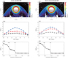 |
Fig. 3 Equatorial distribution of the magnetic field properties around Mercury under quasi-parallel (left) and quasi-perpendicular (right) IMF conditions. (a, a′) Normalised magnetic field strength binned into a grid of 0.1 × 0.1 RM (|Z| < 0.2 RM). (b, b′) Average magnetic field strength just downstream of bow shock (0.8 < F < 1, black), upstream (0 < F < 0.2, red), and downstream (−0.1 RM < robs − rmod < 0 RM, blue) of the magnetopause as a function of the magnetic local time (MLT). (c, c′) Normalised magnetic field strength along the x-axis (11.5 < MLT < 12.5, |Z| < 0.2 RM). The solar wind and magnetosheath data are displayed in the SWI coordinate system, and the magnetosphere data are displayed in the aberrated MSM coordinate system. |
3.3 Magnetic field fluctuations
Figure 5 presents the equatorial plane distribution of the magnetic field fluctuations in Mercury’s space environment. Overall, the amplitude of the magnetic fluctuations is markedly influenced by the cone angle of the IMF. When the IMF is quasi-parallel (Fig. 5a), the fluctuation amplitude is significantly greater than that for the quasi-perpendicular IMF condition (Fig. 5a′). The higher degree of the magnetic fluctuations is primarily observed on the dawnside, which leads to a pronounced dawn-dusk asymmetry. Another key feature is the fluctuation anisotropy, in which transverse fluctuations dominate Mercury’s space environment (Figs. 5c and 5c′).
The spatial distributions of the magnetic fluctuation patterns are similar, as is also shown in the Y–Z plane in Fig. 6. Specifically, two distinct physical regions with enhanced magnetic field fluctuation activity can be identified. The most disrupted magnetic fields are concentrated in the dawnside quasi-parallel bow shock, and the downstream fluctuations are more intense than the upstream fluctuations. This indicates that the quasi-parallel bow-shock region is a significant source of magnetic disturbances. Another pronounced region of magnetic fluctuations is located just outside the tail magnetopause. This suggests that the physical processes in the magnetopause may be another primary source of the magnetic disturbances at Mercury.
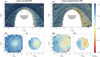 |
Fig. 4 Average magnetic field direction around Mercury’s magnetosphere under quasi-parallel (left) and quasi-perpendicular (right) IMF conditions. (a, a′) Projected magnetic field in the equatorial plane (|Z| < 0.2 RM) in the SWI coordinate system. (b, b′) Projected magnetosheath field just downstream of the shock (0.8 < F < 1) in the terminator plane. (c, c′) Projected magnetosheath field just outside of the magnetopause (0 < F < 0.2). The colour maps show the distribution of the normalised BX binned into a grid of 0.2 × 0.2 RM. |
4 Discussion
Mercury serves as a natural laboratory for conducting comparative studies of planetary space environments due to its proximity to the Sun and its relatively weak planetary magnetic field. In this section, we compare fundamental topics in space science, such as the magnetic field draping, sources of magnetic fluctuations, and the dawn-dusk asymmetries, between Mercury and Earth.
4.1 Magnetic field draping
Magnetic field draping is the process in which the orientation of the magnetosheath field lines changes until they are draped around and compressed against the dayside magnetosphere of a planet. It is particularly relevant to the occurrence and operation of the magnetopause reconnection, and thus, to the interaction of a planetary system with its interplanetary environment. The compression of the magnetic flux at the magnetopause leads to a reduction in plasma density, which forms a plasma depletion layer (PDL) just outside of the dayside magnetopause (Zwan & Wolf 1976). At Earth, this typically occurs under northward IMF conditions.
The formation of a PDL at Mercury was reported by Gershman et al. (2013), who found that subsolar plasma depletion can occur under nearly all upstream conditions at Mercury. Our statistical analysis demonstrated that magnetic field compression occurs throughout the dayside magnetosheath, with a maximum around the subsolar region for both a quasi-parallel and a quasi-perpendicular IMF. A higher compression ratio is observed for a quasi-perpendicular IMF, likely due to greater magnetic field compression at the bow shock and to the more efficient draping under these conditions. Compared with a compression ratio of ~7–8 at Earth (Zhang et al. 2019; Pi et al. 2024), the lower compression ratio of Mercury (~4.8) is attributed to its low Alfvén Mach number. Our results also indicate that the draping and pile-up region radially extends from the subsolar magnetopause to the bow shock, which can also be explained by the low Alfvén Mach number (Zwan & Wolf 1976; Gershman et al. 2013).
The magnetic field draping pattern associated with the IMF cone angle differs between Mercury and Earth. Michotte de Welle et al. (2022) determined the global 3D draping of the magnetic field lines in the dayside magnetosheath of Earth using in situ spacecraft observations and compared them with a magnetostatic draping model assuming no current in the magnetosheath (Kobel & Flückiger 1994). For a quasi-perpendicular (θCA = [45°, 90°]) and extremely radial (θCA = [0°, 12.5°]) IMF, global draping is qualitatively consistent with theoretical magnetostatic draping, whereas in the quasi-parallel IMF regime (θCA = [12.5°, 45°]), the data deviate fundamentally from magnetostatic draping, such that a kink structure forms instead in the quasi-parallel magnetosheath (Michotte de Welle et al. 2022).
At Mercury, however, under quasi-parallel IMF conditions (θCA = [0°, 12.5°]), the observed magnetic divergence centre is consistent with magnetostatic draping. Conversely, under quasi-perpendicular IMF conditions (θCA = [45°, 90°]), a kink of the magnetic field in the magnetosheath is observed. This kink may generate anomalous plasma deflection in the magnetosheath, which is occasionally detected at Earth (Nishino et al. 2008) and is expected to be more prominent in the magnetosheath of Mercury.
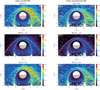 |
Fig. 5 Equatorial distribution of the magnetic fluctuations around Mercury under quasi-parallel (left) and quasi-perpendicular (right) IMF conditions. From top to bottom, the normalised magnetic fluctuation, and its compressional and transverse components, respectively. The solar wind and magnetosheath data are displayed in the SWI coordinate system, and the magnetosphere data are displayed in the aberrated MSM coordinate system. |
4.2 Sources of magnetic fluctuation
Magnetic fluctuation sources in geospace have been studied extensively. Magnetic fluctuations can originate from various sources, including the upstream solar wind, the foreshock, and the magnetopause (Fairfield 1976). Upstream quasi-parallel shocks, the foreshock fluctuations, for instance, 1 Hz whistler waves and transverse magnetosonic waves, can form through interactions between particles that are reflected by the bow shock and incoming solar wind. These waves can transmit across the quasi-parallel shock (Turc et al. 2023), rendering a turbulent magnetosheath and reconnection therein. Magnetosheath jets, predominantly forming downstream of quasi-parallel shocks, also contribute to magnetic fluctuations (Plaschke et al. 2018). These processes result in stronger magnetic fluctuations, especially in transverse mode, both upstream and downstream of the quasi-parallel shock. Processes that occur within the magnetosheath itself are also pivotal in locally generating magnetic field fluctuations (Zastenker et al. 2002). For example, mirror wave modes and ion cyclotron instabilities arise due to the high plasma β and temperature anisotropy that is prevalent in the magnetosheath (Schwartz et al. 1997).
Our findings indicate that the quasi-parallel bow shock of Mercury also serves as a primary source of magnetic fluctuations. It extends across a wide area and propagates downstream, particularly under the radial IMF condition. Various Earth-like ULF waves have indeed been observed in Mercury’s foreshock (Le et al. 2013; Romanelli & DiBraccio 2021). Additionally, the magnetopause region may play a significant role in generating magnetic fluctuations, which is especially visible in the tail region. This likely results from magnetopause processes, such as the magnetopause reconnection, and in particular, the production of flux transfer event (FTE) showers that propagate along the magnetopause (Slavin et al. 2012; Sun et al. 2020; Zhong et al. 2020c), and Kelvin-Helmholtz (K-H) instabilities in the flank region (Sundberg et al. 2012a; Gershman et al. 2015). These phenomena imply that the relatively weak magnetic field of Mercury is highly sensitive to IMF driving.
However, when compared to the magnetosheath of Earth, Mercury’s magnetosheath appears to be a less prominent source of magnetic fluctuations. The order of the magnetosheath field at Mercury is comparatively stable. To date, no definitive observations of compressional-mode mirror waves have been reported. This stability might be attributable to the limited size of Mercury’s magnetosheath and to the significantly lower plasma β, which both inhibit the growth of instabilities or waves.
Within Mercury’s magnetosphere, the dawnside exhibits higher levels of magnetic fluctuations than the duskside. Previous MESSENGER observations have indicated the presence of various ULF waves in the magnetosphere, such as ionBernstein mode waves (Boardsen et al. 2015). These coherent ULF waves tend to exhibit their strongest power on the night-side near the equatorial plane and are more frequent in the pre-midnight sector, with a greater prevalence of compressional waves near the equator (Boardsen et al. 2012). However, our findings demonstrate a dawn-favoured asymmetry in the magnetic fluctuations, particularly in the transverse component. There are several possible explanations for this asymmetry: (1) planet-ward and dawn-ward convection processes that occur within a small-scale length of the magnetotail (Lu et al. 2018; Liu et al. 2019), (2) tail reconnection that is closer to the planet and a higher flux rope generation rate on the dawnside (Zhong et al. 2023), and (3) propagation of the dawnside-favoured magnetosheath fluctuations into the magnetotail, such as solar wind that enters on the dawnside via an upstream-connected window (Zhong et al. 2024). The last of these needs to be confirmed in future investigations.
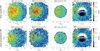 |
Fig. 6 Distribution of magnetic fluctuations in the terminator plane for a quasi-parallel (top) and quasi-perpendicular (bottom) IMF. (a, a′) Solar wind upstream of the bow shock (dBS > 0.2 RM), (b, b′) magnetosheath downstream of the bow shock (0.8 < F < 1), (c, c′) magnetosheath upstream of the magnetopause (0 < F < 0.2), and (d, d′) cross-sectional cut of the tail (−2.5 RM < X < −1.5 RM). The three black circles from the inside out are the Mercury surface, the magnetopause, and the bow shock in the terminator. No data were recorded northward of the magnetosphere in this X range because of the high inclination of the highly eccentric MESSENGER spacecraft orbit. The solar wind and magnetosheath data are displayed in the SWI coordinate system, and the magnetosphere data are displayed in the aberrated MSM coordinate system. |
4.3 Dawn-dusk asymmetries
Dawn-dusk asymmetries are ubiquitous features of the coupled solar wind–magnetosphere system (Walsh et al. 2014). At Earth, these asymmetries in the magnetic environment are primarily attributable to the interaction between the Parker-spiral IMF and the bow shock (Luhmann et al. 1986; Walsh et al. 2012). The IMF Parker spiral orientation forms an angle of 45° with the Sun-Earth line, resulting in distinct bow-shock properties on opposite flanks. The duskside of the magnetosheath typically lies downstream of a quasi-perpendicular shock, leading to a greater magnetic field compression (Zhang et al. 2019), whereas the dawnside is associated with a quasi-parallel shock, which drives more pronounced magnetic fluctuations (Dimmock et al. 2014).
Similarly, Mercury exhibits dawn-favoured asymmetries in magnetic fluctuations, with a typical Parker spiral angle of 30°. However, the asymmetry in the magnetic field strength is less evident at Mercury than at Earth (Zhang et al. 2019). This can be attributed to the significantly lower Alfvén Mach number that is prevalent in the inner heliosphere. The low Alfvén Mach number results in a weak bow shock that is characterised by weak magnetic field compression at the quasi-perpendicular bow shock on the duskside. Additionally, the low Alfvén Mach number leads to a flatter bow-shock geometry. Combined with the typical quasi-radial IMF, the parallel shock region or the resulting foreshock region is expected to extend over a larger local time region.
5 Conclusion
We presented the distinctive characteristics of the global magnetic field morphology and fluctuations in Mercury’s space envirnoment. The magnetic environment is characterised by strong transverse mode-dominated fluctuations for a typical Parker-spiral IMF. When they are subjected to a quasi-perpendicular IMF, the magnetic fluctuations decrease, and the magnetic field strength is compressed more strongly throughout the bow shock, magnetosheath, and magnetosphere. Compared to Earth, Mercury also exhibits a profound dawn-dusk asymmetry in its magnetic fluctuations, but this asymmetry is less significant in terms of magnetic field strength. Unlike Earth, Mercury lacks significant magnetosheath-generated sources of magnetic fluctuations. The magnetic field draping pattern associated with the IMF cone angle differs between Mercury and Earth. These unique features are influenced by Mercury’s relatively small-scale system and the upstream solar wind conditions in close proximity to the Sun, including the low Alfvén Mach number and radial direction of the IMF. These results illustrate the intrinsic value of studying the magnetosphere of Mercury and its dynamics, because Mercury’s space environment presents a unique regime of plasmas and shock conditions that is rarely observed elsewhere in the Solar System. The dual spacecraft orbital mission BepiColombo (Milillo et al. 2020; Benkhoff et al. 2021; Heyner et al. 2021) will greatly enhance our understanding of the space environment of Mercury in the future.
Acknowledgements
This work was supported by the B-type Strategic Priority Program of the Chinese Academy of Sciences (grant No. XDB41000000), the National Natural Science Foundation of China (42388101, 42174217). MESSEN GER MAG and FIPS data are available through NASA’s Planetary Data System (https://pds-ppi.igpp.ucla.edu/). The list of Mercury’s bow shock and magnetopause crossings used in this paper is available in the Zenodo repository (https://doi.org/10.5281/zenodo.13958819).
References
- Aizawa, S., Griton, L. S., Fatemi, S., et al. 2021, Planet. Space Sci., 198, 105176 [NASA ADS] [CrossRef] [Google Scholar]
- Anderson, B. J., Acuña, M. H., Lohr, D. A., et al. 2007, Space Sci. Rev., 131, 417 [CrossRef] [Google Scholar]
- Anderson, B. J., Johnson, C. L., Korth, H., et al. 2011, Science, 333, 1859 [NASA ADS] [CrossRef] [Google Scholar]
- Anderson, B. J., Johnson, C. L., Korth, H., et al. 2012, J. Geophys. Res., 117, E00L12 [Google Scholar]
- Ballerini, G., Lavorenti, F., Califano, F., & Henri, P. 2024, A&A, 687, A204 [NASA ADS] [CrossRef] [EDP Sciences] [Google Scholar]
- Benkhoff, J., Murakami, G., Baumjohann, W., et al. 2021, Space Sci. Rev., 217, 90 [NASA ADS] [CrossRef] [Google Scholar]
- Boardsen, S. A., Slavin, J. A., Anderson, B. J., et al. 2012, J. Geophys. Res (Space Phys.), 117, A00M05 [NASA ADS] [CrossRef] [Google Scholar]
- Boardsen, S. A., Kim, E. H., Raines, J. M., et al. 2015, J. Geophys. Res. (Space Phys.), 120, 4213 [CrossRef] [Google Scholar]
- Burlaga, L. F. 2001, Planet. Space Sci., 49, 1619 [CrossRef] [Google Scholar]
- Chang, Q., Xu, X., Xu, Q., et al. 2019, ApJ, 884, 102 [NASA ADS] [CrossRef] [Google Scholar]
- Chen, Y.-W., Shue, J.-H., Zhong, J., & Shen, H.-W. 2023, ApJ, 957, 26 [NASA ADS] [CrossRef] [Google Scholar]
- Dewey, R. M., Slavin, J. A., Raines, J. M., Azari, A. R., & Sun, W. 2020, J. Geophys. Res. (Space Phys.), 125, e2020JA028112 [CrossRef] [Google Scholar]
- DiBraccio, G. A., Slavin, J. A., Imber, S. M., et al. 2015, Planet. Space Sci., 115, 77 [NASA ADS] [CrossRef] [Google Scholar]
- Dimmock, A. P., Nykyri, K., & Pulkkinen, T. I. 2014, J. Geophys. Res. (Space Phys.), 119, 6231 [NASA ADS] [CrossRef] [Google Scholar]
- Dimmock, A. P., Nykyri, K., Osmane, A., Karimabadi, H., & Pulkkinen, T. I. 2017, Dawn-Dusk Asymmetries of the Earth’s Dayside Magnetosheath in the Magnetosheath Interplanetary Medium Reference Frame (American Geophysical Union (AGU)), 49 [Google Scholar]
- Dong, C., Jin, M., Lingam, M., et al. 2018, PNAS, 115, 260 [NASA ADS] [CrossRef] [Google Scholar]
- Dong, C., Wang, L., Hakim, A., et al. 2019, Geophys. Res. Lett., 46, 11584 [NASA ADS] [CrossRef] [Google Scholar]
- Exner, W., Heyner, D., Liuzzo, L., et al. 2018, Planet. Space Sci., 153, 89 [NASA ADS] [CrossRef] [Google Scholar]
- Exner, W., Simon, S., Heyner, D., & Motschmann, U. 2020, J. Geophys. Res (Space Phys.), 125, e2019JA027691 [Google Scholar]
- Exner, W., Griton, L. S., & Heyner, D. 2024, J. Geophys. Res. (Space Phys.), 129, e2023JA032248 [NASA ADS] [CrossRef] [Google Scholar]
- Fairfield, D. H. 1976, Rev. Geophys., 14, 117 [NASA ADS] [CrossRef] [Google Scholar]
- Gershman, D. J., Slavin, J. A., Raines, J. M., et al. 2013, J. Geophys. Res. (Space Phys.), 118, 2013JA019244 [Google Scholar]
- Gershman, D. J., Raines, J. M., Slavin, J. A., et al. 2015, J. Geophys. Res. (Space Phys.), 120, 4354 [NASA ADS] [CrossRef] [Google Scholar]
- Griton, L., Issautier, K., Moncuquet, M., et al. 2023, A&A, 670, A174 [NASA ADS] [CrossRef] [EDP Sciences] [Google Scholar]
- He, M., Vogt, J., Heyner, D., & Zhong, J. 2017, J. Geophys. Res. (Space Phys.), 122, 6150 [NASA ADS] [CrossRef] [Google Scholar]
- Heyner, D., Nabert, C., Liebert, E., & Glassmeier, K.-H. 2016, J. Geophys. Res. (Space Phys.), 121, 2935 [CrossRef] [Google Scholar]
- Heyner, D., Auster, H. U., Fornaçon, K. H., et al. 2021, Space Sci. Rev., 217, 52 [CrossRef] [Google Scholar]
- Imber, S. M., & Slavin, J. A. 2017, J. Geophys. Res. (Space Phys.), 122, 11402 [NASA ADS] [Google Scholar]
- Ip, W.-H., & Kopp, A. 2002, J. Geophys. Res. (Space Phys.), 107, 1348 [NASA ADS] [Google Scholar]
- James, M. K., Imber, S. M., Bunce, E. J., et al. 2017, J. Geophys. Res. (Space Phys.), 122, 7907 [NASA ADS] [CrossRef] [Google Scholar]
- James, M. K., Imber, S. M., Yeoman, T. K., & Bunce, E. J. 2019, J. Geophys. Res. (Space Phys.), 124, 211 [CrossRef] [Google Scholar]
- Jia, X., Slavin, J. A., Gombosi, T. I., et al. 2015, J. Geophys. Res. (Space Phys.), 120, 2015JA021143 [Google Scholar]
- Jia, X., Slavin, J. A., Poh, G., et al. 2019, J. Geophys. Res. (Space Phys.), 124, 229 [NASA ADS] [CrossRef] [Google Scholar]
- Kallio, E., Jarvinen, R., Massetti, S., et al. 2022, Geophys. Res. Lett., 49, 2022GL101850 [NASA ADS] [CrossRef] [Google Scholar]
- Kobel, E., & Flückiger, E. O. 1994, J. Geophys. Res. (Space Phys.), 99, 23617 [NASA ADS] [CrossRef] [Google Scholar]
- Lavorenti, F., Henri, P., Califano, F., et al. 2022, A&A, 664, A133 [NASA ADS] [CrossRef] [EDP Sciences] [Google Scholar]
- Le, G., Chi, P. J., Blanco-Cano, X., et al. 2013, J. Geophys. Res. (Space Phys.), 118, 2809 [CrossRef] [Google Scholar]
- Liljeblad, E., & Karlsson, T. 2017, Ann. Geophys., 35, 879 [NASA ADS] [CrossRef] [Google Scholar]
- Liu, Y.-H., Li, T. C., Hesse, M., et al. 2019, J. Geophys. Res. (Space Phys.), 124, 2819 [NASA ADS] [CrossRef] [Google Scholar]
- Lu, S., Pritchett, P. L., Angelopoulos, V., & Artemyev, A. V. 2018, J. Geophys. Res. (Space Phys.), 123, 2801 [NASA ADS] [CrossRef] [Google Scholar]
- Lu, Q., Guo, J., Lu, S., et al. 2022, ApJ, 937, 1 [NASA ADS] [CrossRef] [Google Scholar]
- Luhmann, J. G., Russell, C. T., & Elphic, R. C. 1986, J. Geophys. Res. (Space Phys.), 91, 1711 [NASA ADS] [CrossRef] [Google Scholar]
- Masters, A., Slavin, J. A., DiBraccio, G. A., et al. 2013, J. Geophys. Res. (Space Phys.), 118, 4381 [NASA ADS] [CrossRef] [Google Scholar]
- Michotte de Welle, B., Aunai, N., Nguyen, G., et al. 2022, J. Geophys. Res. (Space Phys.), 127, e2022JA030996 [NASA ADS] [CrossRef] [Google Scholar]
- Milillo, A., Fujimoto, M., Murakami, G., et al. 2020, Space Sci. Rev., 216, 93 [NASA ADS] [CrossRef] [Google Scholar]
- Ness, N. F., Behannon, K. W., Lepping, R. P., & Whang, Y. C. 1975, Nature, 255, 204 [NASA ADS] [CrossRef] [Google Scholar]
- Nishino, M. N., Fujimoto, M., Phan, T.-D., et al. 2008, Phys. Rev. Lett., 101, 065003 [CrossRef] [Google Scholar]
- Orsini, S., Blomberg, L. G., Delcourt, D., et al. 2007, Space Sci. Rev., 132, 551 [NASA ADS] [CrossRef] [Google Scholar]
- Paral, J., Trávníček, P. M., Rankin, R., & Schriver, D. 2010, Geophys. Res. Lett., 37, L19102 [NASA ADS] [CrossRef] [Google Scholar]
- Pi, G., Němeček, Z., Safrankova, J., & Grygorov, K. 2024, Front. Astron. Space Sci., 11, 1401078 [NASA ADS] [CrossRef] [Google Scholar]
- Plaschke, F., Hietala, H., Archer, M., et al. 2018, Space Sci. Rev., 214, 81 [NASA ADS] [CrossRef] [Google Scholar]
- Poh, G., Slavin, J. A., Jia, X., et al. 2017, J. Geophys. Res. (Space Phys.), 122, 8419 [NASA ADS] [CrossRef] [Google Scholar]
- Romanelli, N., & DiBraccio, G. A. 2021, Nat. Commun., 12, 6748 [NASA ADS] [CrossRef] [Google Scholar]
- Schmid, D., Narita, Y., Plaschke, F., et al. 2021, Geophys. Res. Lett., 48, e2021GL092606 [CrossRef] [Google Scholar]
- Schwartz, S. J., Burgess, D., & Moses, J. J. 1997, Ann. Geophys., 14, 1134 [NASA ADS] [Google Scholar]
- Shue, J. H., Chao, J. K., Fu, H. C., et al. 1997, J. Geophys. Res. (Space Phys.), 102, 9497 [NASA ADS] [CrossRef] [Google Scholar]
- Slavin, J. A., Anderson, B. J., Zurbuchen, T. H., et al. 2009, Geophys. Res. Lett., 36, L02101 [Google Scholar]
- Slavin, J. A., Imber, S. M., Boardsen, S. A., et al. 2012, J. Geophys. Res. (Space Phys.), 117, A00M06 [NASA ADS] [Google Scholar]
- Slavin, J. A., Imber, S. M., & Raines, J. M. 2021, A Dungey Cycle in the Life of Mercury’s Magnetosphere, 2 (Magnetospheres in the Solar System: AGU) [Google Scholar]
- Smith, A. W., Slavin, J. A., Jackman, C. M., Poh, G. K., & Fear, R. C. 2017, J Geophys. Res. (Space Phys.), 122, 8136 [NASA ADS] [CrossRef] [Google Scholar]
- Solomon, S., McNutt, R. L., Gold, R., & Domingue, D. 2007, Space Sci. Rev., 131, 3 [NASA ADS] [CrossRef] [Google Scholar]
- Solomon, S. C., Nittler, L. R., & Anderson, B. J. 2018, Mercury: The View after MESSENGER, Cambridge Planetary Science (Cambridge University Press) [CrossRef] [Google Scholar]
- Sun, W.-J., Slavin, J. A., Fu, S., et al. 2015, Geophys. Res. Lett., 42, 6189 [NASA ADS] [CrossRef] [Google Scholar]
- Sun, W. J., Fu, S. Y., Slavin, J. A., et al. 2016, J. Geophys. Res. (Space Phys.), 121, 7590 [CrossRef] [Google Scholar]
- Sun, W. J., Slavin, J. A., Smith, A. W., et al. 2020, Geophys. Res. Lett., 47, e2020GL089784 [CrossRef] [Google Scholar]
- Sundberg, T., Boardsen, S. A., Slavin, J. A., et al. 2012a, J. Geophys. Res. (Space Phys.), 117, A04216 [Google Scholar]
- Sundberg, T., Slavin, J. A., Boardsen, S. A., et al. 2012b, J. Geophys. Res. (Space Phys.), 117, A00M03 [NASA ADS] [Google Scholar]
- Sundberg, T., Boardsen, S. A., Burgess, D., & Slavin, J. A. 2015, J. Geophys. Res. (Space Phys.), 120, 7342 [NASA ADS] [CrossRef] [Google Scholar]
- Trávníček, P. M., Schriver, D., Hellinger, P., et al. 2010, Icarus, 209, 11 [CrossRef] [Google Scholar]
- Turc, L., Roberts, O. W., Verscharen, D., et al. 2023, Nat. Phys., 19, 78 [NASA ADS] [CrossRef] [Google Scholar]
- Verigin, M. I., Tátrallyay, M., Erdos, G., & Kotova, G. A. 2006, Adv. Space Res., 37, 515 [NASA ADS] [CrossRef] [Google Scholar]
- Vernisse, Y., Riousset, J. A., Motschmann, U., & Glassmeier, K. H. 2017, Planet. Space Sci., 137, 40 [NASA ADS] [CrossRef] [Google Scholar]
- Walsh, B. M., Sibeck, D. G., Wang, Y., & Fairfield, D. H. 2012, J. Geophys. Res. (Space Phys.), 117 [Google Scholar]
- Walsh, A. P., Haaland, S., Forsyth, C., et al. 2014, Ann. Geophys., 32, 705 [NASA ADS] [CrossRef] [Google Scholar]
- Wang, Y., Zhong, J., Slavin, J., et al. 2023, Geophys. Res. Lett., 50, e2022GL102574 [NASA ADS] [CrossRef] [Google Scholar]
- Winslow, R. M., Anderson, B. J., Johnson, C. L., et al. 2013, J. Geophys. Res. (Space Phys.), 118, 2213 [NASA ADS] [CrossRef] [Google Scholar]
- Zastenker, G. N., Nozdrachev, M. N., Němeček, Z., et al. 2002, Planet. Space Sci., 50, 601 [CrossRef] [Google Scholar]
- Zhang, H., Fu, S., Pu, Z., et al. 2019, ApJ, 880, 122 [NASA ADS] [CrossRef] [Google Scholar]
- Zhong, J., Wan, W. X., Slavin, J. A., et al. 2015a, J. Geophys. Res. (Space Phys.), 120, 7658 [NASA ADS] [CrossRef] [Google Scholar]
- Zhong, J., Wan, W. X., Wei, Y., et al. 2015b, Geophys. Res. Lett., 42, 10135 [NASA ADS] [CrossRef] [Google Scholar]
- Zhong, J., Wei, Y., Pu, Z. Y., et al. 2018, ApJ, 860, L20 [NASA ADS] [CrossRef] [Google Scholar]
- Zhong, J., Zong, Q. G., Wei, Y., et al. 2019, ApJ, 886, L32 [NASA ADS] [CrossRef] [Google Scholar]
- Zhong, J., Lee, L. C., Wang, X. G., et al. 2020a, ApJ, 893, L11 [NASA ADS] [CrossRef] [Google Scholar]
- Zhong, J., Shue, J. H., Wei, Y., et al. 2020b, ApJ, 892, 2 [NASA ADS] [CrossRef] [Google Scholar]
- Zhong, J., Wei, Y., Lee, L. C., et al. 2020c, ApJ, 893, L18 [NASA ADS] [CrossRef] [Google Scholar]
- Zhong, J., Lee, L.-C., Slavin, J. A., Zhang, H., & Wei, Y. 2023, J. Geophys. Res. (Space Phys.), 128, e2022JA031134 [NASA ADS] [CrossRef] [Google Scholar]
- Zhong, J., Xie, L., Lee, L.-C., et al. 2024, Geophys. Res. Lett., 51, e2023GL106266 [NASA ADS] [CrossRef] [Google Scholar]
- Zwan, B. J., & Wolf, R. A. 1976, J. Geophys. Res., 81, 1636 [NASA ADS] [CrossRef] [Google Scholar]
All Figures
|
Fig. 1 Example of a MESSENGER orbital observation of the magnetic properties around Mercury. (a, b) Magnetic field magnitude and its three components in the aberrated MSM coordinates. (c) Magnetic fluctuation and its compressional/transversal components. (d) Spectrogram of the ion differential energy flux (cm−2 sr−1 s−1 keV−1). The horizontal green, red, and blue bars label the solar wind (SW), magnetosheath (MSH), and magnetosphere (MSP) regions, respectively. (e) and (f) MESSENGER orbit projected onto the equatorial and noon-midnight planes relative to the Mercury surface (circle) and the average magnetopause (MP) and bow shock (BS) from the model (Zhong et al. 2015a). |
| In the text | |
|
Fig. 2 Distribution of 15-minute averaged IMF cone angle (a) and intensity (b) upstream of the bow shock during the whole MESSENGER mission. The overall histogram of the cone angle is separated into two histograms according to the sign of BY (blue: negative; red: positive), and the magnetic field intensity is separated into two histograms according to the cone angle (blue: |90° − θCA| > 45°; red: |90° − θCA| < 45°). |
| In the text | |
|
Fig. 3 Equatorial distribution of the magnetic field properties around Mercury under quasi-parallel (left) and quasi-perpendicular (right) IMF conditions. (a, a′) Normalised magnetic field strength binned into a grid of 0.1 × 0.1 RM (|Z| < 0.2 RM). (b, b′) Average magnetic field strength just downstream of bow shock (0.8 < F < 1, black), upstream (0 < F < 0.2, red), and downstream (−0.1 RM < robs − rmod < 0 RM, blue) of the magnetopause as a function of the magnetic local time (MLT). (c, c′) Normalised magnetic field strength along the x-axis (11.5 < MLT < 12.5, |Z| < 0.2 RM). The solar wind and magnetosheath data are displayed in the SWI coordinate system, and the magnetosphere data are displayed in the aberrated MSM coordinate system. |
| In the text | |
|
Fig. 4 Average magnetic field direction around Mercury’s magnetosphere under quasi-parallel (left) and quasi-perpendicular (right) IMF conditions. (a, a′) Projected magnetic field in the equatorial plane (|Z| < 0.2 RM) in the SWI coordinate system. (b, b′) Projected magnetosheath field just downstream of the shock (0.8 < F < 1) in the terminator plane. (c, c′) Projected magnetosheath field just outside of the magnetopause (0 < F < 0.2). The colour maps show the distribution of the normalised BX binned into a grid of 0.2 × 0.2 RM. |
| In the text | |
|
Fig. 5 Equatorial distribution of the magnetic fluctuations around Mercury under quasi-parallel (left) and quasi-perpendicular (right) IMF conditions. From top to bottom, the normalised magnetic fluctuation, and its compressional and transverse components, respectively. The solar wind and magnetosheath data are displayed in the SWI coordinate system, and the magnetosphere data are displayed in the aberrated MSM coordinate system. |
| In the text | |
|
Fig. 6 Distribution of magnetic fluctuations in the terminator plane for a quasi-parallel (top) and quasi-perpendicular (bottom) IMF. (a, a′) Solar wind upstream of the bow shock (dBS > 0.2 RM), (b, b′) magnetosheath downstream of the bow shock (0.8 < F < 1), (c, c′) magnetosheath upstream of the magnetopause (0 < F < 0.2), and (d, d′) cross-sectional cut of the tail (−2.5 RM < X < −1.5 RM). The three black circles from the inside out are the Mercury surface, the magnetopause, and the bow shock in the terminator. No data were recorded northward of the magnetosphere in this X range because of the high inclination of the highly eccentric MESSENGER spacecraft orbit. The solar wind and magnetosheath data are displayed in the SWI coordinate system, and the magnetosphere data are displayed in the aberrated MSM coordinate system. |
| In the text | |
Current usage metrics show cumulative count of Article Views (full-text article views including HTML views, PDF and ePub downloads, according to the available data) and Abstracts Views on Vision4Press platform.
Data correspond to usage on the plateform after 2015. The current usage metrics is available 48-96 hours after online publication and is updated daily on week days.
Initial download of the metrics may take a while.