| Issue |
A&A
Volume 687, July 2024
|
|
|---|---|---|
| Article Number | A243 | |
| Number of page(s) | 10 | |
| Section | Planets and planetary systems | |
| DOI | https://doi.org/10.1051/0004-6361/202449450 | |
| Published online | 23 July 2024 | |
Structure and dynamics of the Hermean magnetosphere revealed by electron observations from the Mercury electron analyzer after the first three Mercury flybys of BepiColombo
1
IRAP, CNRS-UPS-CNES,
Toulouse,
France
e-mail: This email address is being protected from spambots. You need JavaScript enabled to view it.
2
Institut Supérieur de l’Aéronautique et de l’Espace (ISAE-SUPAERO), Université de Toulouse,
Toulouse,
France
3
Institute of Space and Astronautical Science, Japan Aerospace Exploration Agency,
Sagamihara,
Japan
4
University of Pisa,
Pisa,
Italy
5
Laboratoire de Physique des Plasmas (LPP), CNRS-Observatoire de Paris Sorbonne Université – Université Paris Saclay-Ecole Polytechnique – Institut Polytechnique de Paris,
91120
Palaiseau,
France
6
Department of Geophysics, Graduate School of Science, Kyoto University,
Kyoto,
Japan
7
AKKODIS,
Blagnac,
France
8
Swedish Institute of Space Physics,
Uppsala,
Sweden
9
Department of Earth and Space Science, Graduate School of Science, Osaka University,
Osaka,
Japan
10
Max Planck Institute for Solar System Research,
Göttingen,
Germany
Received:
1
February
2024
Accepted:
27
April
2024
Abstract
Context. The Mercury electron analyzer (MEA) obtained new electron observations during the first three Mercury flybys by BepiColombo on October 1, 2021 (MFB1), June 23 , 2022 (MFB2), and June 19, 2023 (MFB3). BepiColombo entered the dusk side magnetotail from the flank magnetosheath in the northern hemisphere, crossed the Mercury solar orbital equator around midnight in the magnetotail, traveled from midnight to dawn in the southern hemisphere near the closest approach, and exited from the post-dawn magnetosphere into the dayside magnetosheath.
Aims. We aim to identify the magnetospheric boundaries and describe the structure and dynamics of the electron populations observed in the various regions explored along the flyby trajectories.
Methods. We derive 4s time resolution electron densities and temperatures from MEA observations. We compare and contrast our new BepiColombo electron observations with those obtained from the Mariner 10 scanning electron spectrometer (SES) 49 yr ago.
Results. A comparison to the averaged magnetospheric boundary crossings of MESSENGER indicates that the magnetosphere of Mercury was compressed during MFB1, close to its average state during MFB2, and highly compressed during MFB3. Our new MEA observations reveal the presence of a wake effect very close behind Mercury when BepiColombo entered the shadow region, a significant dusk-dawn asymmetry in electron fluxes in the nightside magnetosphere, and strongly fluctuating electrons with energies above 100s eV in the dawnside magnetosphere. Magnetospheric electron densities and temperatures are in the range of 10–30 cm−3 and above a few 100s eV in the pre-midnight-sector, and in the range of 1–100 cm−3 and well below 100 eV in the post-midnight sector, respectively.
Conclusions. The MEA electron observations of different solar wind properties encountered during the first three Mercury flybys reveal the highly dynamic response and variability of the solar wind-magnetosphere interactions at Mercury. A good match is found between the electron plasma parameters derived by MEA in the various regions of the Hermean environment and similar ones derived in a few cases from other instruments on board BepiColombo.
Key words: plasmas / instrumentation: detectors / planets and satellites: detection
© The Authors 2024
 Open Access article, published by EDP Sciences, under the terms of the Creative Commons Attribution License (https://creativecommons.org/licenses/by/4.0), which permits unrestricted use, distribution, and reproduction in any medium, provided the original work is properly cited.
This article is published in open access under the Subscribe to Open model. This email address is being protected from spambots. You need JavaScript enabled to view it. to support open access publication.
1 Introduction
The space exploration of Mercury started with the Mariner 10 mission launched by NASA on November 2, 1973. Of its three encounters with Mercury, two were sufficiently close to allow the study of the planetary system on its own. During its first flyby on March 29, 1974 and third one on March 16, 1975, the spacecraft flew from the southern hemisphere of Mercury to the northern one, crossing the equatorial plane around the midnight sector and flowing over the northern polar region, respectively. Mariner 10 carried a fluxgate magnetometer and two plasma science instruments. The latter were composed of the scanning electrostatic analyzer (SEA) measuring ions and electrons in the sunward direction, and the scanning electron spectrometer (SES) measuring electrons between 13 and 700 eV in the anti-sunward direction (Ogilvie et al. 1977). However, technical issues on the SEA made plasma measurements possible only with the SES (Ogilvie et al. 1977). Despite this limitation, the combination of electron and magnetic field measurements allowed operators to detect the presence of an intrinsic magnetic field at Mercury as well as the existence of a magnetosphere similar to that of the Earth but smaller in size. In particular, SES measurements showed that the electron moments inside the magnetosphere of Mercury differed from those of the surrounding solar wind (SW), with magnetospheric densities estimated to be around 1 cm−3 and magnetospheric temperatures estimated to be around 20–40 eV and 200 eV in the cool and hot plasma sheets, respectively.
The first spacecraft to orbit Mercury, MESSENGER (MErcury Surface, Space ENvironment, GEochemistry, and Ranging), was launched by NASA on August 3, 2004. Observations from MESSENGER’s highly elliptical orbits (9300 × 200 km) during the time period from 2011 to 2015 enabled statistical studies of the plasma properties in the magnetosphere of Mercury. Zhao et al. (2020) analyzed 5 yr of ion moments obtained in the 50 eV q−1 to 20 keV q−1 energy per charge range from the fast imaging plasma spectrometer (FIPS) together with magnetic field measurements obtained from the magnetometer (MAG) on board MESSENGER, and report a significant dusk-dawn asymmetry, with higher values on the dawnside for the density and pressure of protons, the most abundant ion species. They also report that in the nightside equatorial magnetosphere of Mercury the density of protons reaches a maximum average of 4 cm−3.
In this paper, we summarize electron plasma observations obtained during the first three Mercury flybys of the Bepi-Colombo mission by the Mercury Electron Analyzer (MEA) of the Mercury Plasma Particle Experiment (Saito et al. 2021) on board the Mio spacecraft. The MEA consists of two top-hat electrostatic analyzers that measure, during those flybys, electrons between 3 and 3000 eV for MEA1 and between 3 and 27 000 eV for MEA2. Each sensor includes microchannel plate (MCP) detectors in a chevron stack configuration with 16 discrete anodes (or sectors) of 22.5° resolution in azimuth. During the cruise phase of BepiColombo, MEA works in a low-resolution telemetry mode (L-mode), in which an energy sweep consists of only 16 discretized energy bins. The data products used in the present study are electron omnidirectional fluxes (Et-OMN, hereinafter referred to as OMNI, available for both MEA1 and MEA2) and full 3D electron distribution (hereinafter referred to as 3D, only available for MEA1). In L-mode, the OMNI combine all the counts of the different sectors with a time resolution of 4 s, whereas 3D enables one to obtain a complete angular energy spectrum with a time resolution of 640 s. However, the magnetospheric orbiter sunshield and interface structure (MOSIF) partially obstructs the field of view (FoV) of MEA during the cruise phase of BepiColombo, and therefore only two sectors for each sensor can detect electrons in free space and are used to estimate their parameters (Rojo et al. 2023).
The aim of this paper is to compare and contrast the first electron parameters derived from MEA observations during each of the first three Mercury flybys of BepiColombo (hereinafter referred to as MFB1, MFB2, and MFB3) as well as those deduced 49 yr ago with the SES instrument of Mariner 10 during its first Mercury flyby (hereinafter referred to as M10 FB1). Section 2 summarizes the geometric properties of the different encounters with Mercury. Section 3 gives an overview of the different regions crossed by BepiColombo and Mariner 10 identified from their respective energy-time electron count rate spectra. Section 4 shows and compares the electron density and temperature profiles obtained for each flyby. Section 5 put our results into the context of observations from MESSENGER, Parker Solar Probe (PSP), and complementary instruments on board BepiColombo. Section 6 concludes our study.
2 Geometrical properties of the BepiColombo flybys
The first three Mercury flybys occurred during the cruise phase of BepiColombo in which the two spacecraft, Mio and the Mercury Planetary Orbiter (MPO), were stacked together with the Mercury Transfer Module (MTM) (Murakami et al. 2020). The same side of the spacecraft is always pointing sunward during the entire cruise phase. Figure 1 shows the geometries of BepiColombo’s first three Mercury flybys and compares them with the geometry of the first flyby of Mariner 10. This choice is motivated by the close similarity of their trajectories. The trajectories are represented in the Mercury solar orbital (MSO) coordinate system, where X points at the Sun, -Y points in the orbital direction of Mercury, and Z completes the right-hand set and points northward. The closest approach (CA) took place at 23:34 UTC on October 1, 2021 at an altitude of 199 km above the planet’s surface for MFB1, at 09:44 UTC on June 23, 2022 at an altitude of 200 km for MFB2, at 19:34 UTC on June 19, 2023 at an altitude of 236 km for MFB3, and at 20:47 UTC on March, 29 1974 at an altitude of 703 km for M10 FB1. The corresponding heliocentric distances of Mercury to the Sun are 0.380, 0.378, 0.326, and 0.46 astronomical units (AU) for MFB1, MFB2, MFB3, and M10 FB1, respectively. As is seen in Fig. 1, BepiColombo entered the dusk side (YMSO > 0) magnetotail (XMSO < 0) from the flank magnetosheath in the northern MSO hemisphere (ZMSO > 0), crossed the MSO equator (ZMSO = 0) around midnight (YMSO ≈ 0 and XMSO < 0) in the magnetotail, traveled from midnight to dawn (YMSO < 0) in the southern MSO hemisphere (ZMSO < 0) near CA, and exited from the post-dawn magnetosphere into the dayside magnetosheath (XMSO > 0) during MFB1, MFB2, and MFB3. Contrary to Bepi-Colombo, Mariner 10 crossed Mercury’s magnetotail from the southern to the northern hemisphere during M10 FB1.
3 Overview of magnetospheric regions crossed by BepiColombo
Figure 2 shows energy-distance electron spectrograms obtained by MEA 1 during MFB1, MFB2, and MFB3, and compares them with the electron spectrogram obtained by the SES instrument during M10 FB1. The electron spectrograms are displayed as a function of the distance along the YMSO axis in order to take advantage of the similarity between the spacecraft trajectories and make the comparison of the magnetospheric regions crossed by the spacecraft easier. Since all spacecraft entered the Hermean magnetosphere from the dusk side (YMSO > 0), times increase from right to left. Except for MFB1, all the boundaries crossed by BepiColombo were directly determined from the electron spectra obtained by MEA1. Due to a telemetry data gap during MFB1, no inbound BS crossing was directly measured by MEA. The inbound BS and MP and outbound MP crossings were determined with the help of the Mercury Ion Analyzer (MIA) and the Energetic Neutral atom Analyzer (ENA) of MPPE. Here, they were extracted from Harada et al. (2022) and Aizawa et al. (2023). During MFB2, MEA1 could not observe the inbound bow shock (BS) as the trajectory of BepiColombo had an angle of −45° with respect to the XMSO axis in the XY plane. For M10 FB1, the boundaries were extracted from Ogilvie et al. (1974), in which they identified the boundary crossings with the help of the magnetometer. All the times of the different boundary crossings identified are listed in Table 1.
During M10 FB1, SES recorded the main characteristics of the Hermean magnetospheric environment. The electron fluxes were the most intense in the magnetosheath, where the plasma is compressed and heated. The observed energy of the electrons in the nightside (dayside) magnetosheath is similar (higher) than the energy of the electrons in the SW, respectively. In the magnetosphere, a dusk-dawn asymmetry was observed on the nightside. Whereas MEA confirmed those tendencies 49 years after the measurements of SES, the new BepiColombo electron observations also highlighted particular features.
The first one is what could be a wake effect very close behind Mercury, measured when BepiColombo entered the shadow region. The strong electron depletion observed there is similar to those reported for the THEMIS mission by Xu et al. (2019) and Tao et al. (2012) in the lunar wake. However, during the wake crossing, the Electric Field Instrument (EFI) of ARTEMIS P1 is biased in such a way that the spacecraft potential is maintained to +2 Volts, as was reported by Halekas et al. (2014). This way, it ensures that the electron depletion is due to the lunar wake and not the negative spacecraft potential that would normally affect a platform in the shadow region. This technique is not possible in the cruise phase configuration, so the nature of this observation will be settled during the nominal science phase of the mission.
The second feature is that observations obtained during MFB1 contrast with those obtained during the other two Mercury flybys, since no dusk-dawn asymmetry in electron fluxes was observed on the nightside. Indeed, electrons with similar energies were observed on both sides of the planet during MFB1, albeit with a weaker count rate intensity observed on the dusk side compared to the dawn side due to the different distances to the planet. The observed count rates nevertheless remained very high compared to those observed during MFB2 and MFB3 at equivalent distances to the planet.
The third feature is the systematic observation on the dawn side of electrons with energies above 100s eV, more pronounced during MFB2 and MFB3. These high-energy electrons were observed as transient pulses during MFB2, whereas they were continuously measured until the outbound magnetopause (MP) during MFB3. These high-energy electrons could not be fully detected by SES on board Mariner 10 since the upper energy limit of this instrument (700 eV) was below the peak energy of these electrons. A deeper analysis of these high-energy electrons revealed energy-time dispersed electron enhancements supporting the occurrence of multiple substorm-related, impulsive injections of electrons during MFB1, as has been shown by Aizawa et al. (2023), electrons accelerated by field-aligned potentials during MFB2 (Aizawa et al. 2024), and the likely observation of highly dynamic and fluctuating electron populations within the plasma sheet during MFB3.
The fourth feature is the observation of a significantly lower SW electron peak energy (20–30 eV), and hence a weaker electron temperature is expected with SES than the SW electron peak energy (50 eV on average) observed with MEA. The latter is consistent with Whittlesey et al. (2020), who reported at the orbital location of Mercury an energy peak in the 40–60 eV range or above.
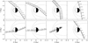 |
Fig. 1 Geometry of the flybys from BepiColombo and Mariner 10 in the MSO coordinate system with average BS and MP models displayed with dashed gray lines. The origin of the MSO coordinate system is at the planetary center of mass, +X is sunward, +Y lies in the orbital plane, perpendicular to +X and opposite to the direction of planetary orbital motion (i.e., +Y is positive toward dusk), and +Z is normal to the orbital plane and positive northward. From left to right: MFB1 (October 1, 2021), MFB2 (June 23, 2022), MFB3 (June 19, 2023), and M10 FB1 (March 29, 1974). Top: trajectories in the XY plane. Bottom: trajectories in the XZ plane. Distances to the planet are given in Mercury radii, 1 RM = 2440 km. The marks are the time in UTC (HH:MM). |
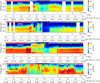 |
Fig. 2 Energy-distance spectrograms of electron count rates displayed as a function of the distance along the YMSO axis. From top to bottom: MEA1 observations for MFB1, MFB2, and MFB3, and SES observations for M10 FB1. The vertical dashed green line delineates the CA. For each flyby, the spacecraft altitude (in Mercury radius) and the time (in UTC, HH:MM) are indicated below the corresponding plot. We note that the time increases from right to left. The red, green, and light and dark blue boxes above the corresponding plot delineate the SW, the magnetosheath, the magnetosphere, and the eclipse (or shadow regions) crossed by the spacecraft for each flyby, respectively. |
Time (in UTC) of the different boundary crossings identified from electron observations during MFB1 (October 1, 2021), MFB2 (June 23, 2022), MFB3 (June 19, 2023), and M10 FB1 (March 29, 1974).
4 Electron parameters: Density and temperature
The procedure used to derive electron density from MEA observations is described in Rojo et al. (2023). The electron parameters are first deduced from MEA1 3D data products. We assume that electrons are isotropic, and assigned to all azimuthal sectors of MEA1 the same count rate as the one observed by the two sectors that have an unobstructed FoV. We first fit the reconstructed electron population with a Maxwellian distribution. We then subtracted the corresponding fit from the observed count rates, and removed the residual count rates that remained at low energy, assuming that they correspond to secondary electron emission. We finally summed the Maxwellian fit and the count rate at high energy before integrating it over energy and deducing the electron parameters. In the present work, we extended the work of Rojo et al. (2023) in order to derive the electron temperature from OMNI data in addition to the electron density. We invite the reader to refer to Appendix A, where this extension is described.
The density and temperature estimates for MFB1, MFB2, MFB3, and M10 FB1 are presented in the same way in Figs. 3 and 4, respectively. The dashed green line and the colored regions are the same as the ones shown in Fig. 2. For Bepi-Colombo, the blue stars and red crosses represent the density or temperature calculated with the 3D and OMNI data, respectively. For MFB2 and MFB3, the observed count rates when BepiColombo entered the eclipse region were too low to reliably apply the fitting procedure described previously, and therefore the corresponding values were not considered.
We first notice that the densities measured by Mariner 10/SES are lower than those measured by BepiColombo/MEA in all the regions crossed by the spacecraft. During MFB3, the SW electron densities are three to four times denser than those measured during MFB1 and MFB2. As has been observed on Earth and other planets, the electrons in the magnetosheath are denser and hotter due to their compression between the BS and the MP. This effect is most clearly noticeable during the outbound magnetosheath crossings, but also during the inbound ones for MFB3 and M10 FB1. For all flybys, the magnetosphere of Mercury appears as a cavity repelling electrons from the SW. In the pre-midnight sector (YMSO > 0 and XMSO < 0), the magnetospheric electron densities remain quite stable, with values between 10 and 30 cm−3 depending on the flyby. As BepiColombo flies closer to the planet in the post-midnight sector, the magnetospheric electron densities fluctuate significantly but differently for each flyby, with values between 1 and 100 cm−3. A similar trend is observed for magnetospheric electron temperatures, with values well above a few 100s eV, except during MFB1. The average temperature of the plasma sheet electrons observed during MFB3 in particular is close to 300 eV.
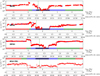 |
Fig. 3 Electron density measured during BepiColombo and Mariner 10 flybys. From top to bottom: electron density profiles for MFB1, MFB2, MFB3, and M10 FB1 displayed as a function of the distance along the YMSO axis. The vertical dashed green line delineates the CA. For each flyby, the spacecraft altitude (in Mercury radius) and the time (in UTC, HH:MM) are indicated below the corresponding plot. We note that the time increases from right to left. The red, green, and light and dark blue boxes below the corresponding plot delineate the SW, the magnetosheath, the magnetosphere, and the eclipse or shadow regions crossed by the spacecraft for each flyby, respectively. The blue stars and red crosses represent the densities deduced from the 3D and OMNI data products of MEA1, respectively. |
5 Discussion
Figure 5 shows a comparison between the positions of the averaged BS and MP crossings of MESSENGER and the ones made by BepiColombo during the three Mercury flybys. The boundaries are represented in an aberrated Mercury solar mag-netospheric (MSM) coordinate system. This accounts for the SW aberration and the northward dipole offset (+0.196 RM on ZMSO). It indicates that the magnetosphere of Mercury was compressed during the outbound leg of MFB1, close to its average state during both the inbound and outbound legs of MFB2, and highly compressed again during the whole MFB3. A fit to the found BS and MP locations using the empirical models from previous studies yields extrapolated outbound standoff BS planetocentric distances of 1.67, 2.03, and 1.62 RM for MFB1, MFB2, and MFB3, respectively, and extrapolated inbound-outbound standoff MP planetocentric distances of 1.40/1.22, 1.00/1.50, and 1.04/1.17 RM for MFB1, MFB2, and MFB3, respectively. These estimated values have to be compared to the mean standoff BS and MP distances derived from MESSENGER observations of 1.90 and 1.45 RM, respectively. The inferred inbound-outbound standoff MP values correspond in the KT17 magnetospheric field model (Korth et al. 2017) to a disturbance index (Dst) of 47/100, 0/100, and 100/100 for MFB1, MFB2, and MFB3, respectively. The estimated SW dynamic pressure calculated by considering both statistical values obtained by MESSENGER observations and a theoretical model of the compression of Mercury’s magnetosphere that includes the effects of induction at Mercury’s core corresponding to the equation shown in Jia et al. (2019) is in the range of 15.05/23.95, 24.27/, and 32.03/32.03 nPa for the inbound-outbound legs of MFB1, MFB2, and MFB3, respectively, which is higher than the most probable dynamic pressure of 10 nPa derived from MESSENGER observations. A summary of all these estimates is given in Table 2.
A comparison of our SW electron densities calculated during MFB1 and MFB2 with those observed in the heliosphere at the orbital distance of Mercury and reported in previous statistical studies (Sun et al. 2022; Dakeyo et al. 2022) shows a good agreement. On the contrary, our SW electron density calculated during MFB3 with values as high as 200 cm−3 exceeds those reported in these studies. However, such high SW density values are reported by Lavraud et al. (2020) during the first orbit of PSP. They point out that a dense SW can be observed during heliospheric plasma sheet or heliospheric current sheet crossings, and we suggest that this was also the case during MFB3. Interestingly, the day before MFB3, PSP was upstream and radially aligned with BepiColombo, and we take advantage of this configuration with two-point measurements in order to confirm our suggestion. The SW electron densities of about 10 cm−3 calculated during M10 FB1 are four to ten times lower than those measured during the three BepiColombo flybys. Contrary to the density, the SW electron temperatures of about 10— 20 eV calculated during M10 FB1 are in close agreement with the statistical values of ≈ 18 eV obtained by Rojo et al. (2023) and Dakeyo et al. (2022). We also note that our inferred SW velocity during the inbound leg of MFB1 agrees with the observation of a slow SW with a speed of around 340 km s−1 reported by Alberti et al. (2023) from the Planetary Ion CAMera (PICAM) instrument on board BepiColombo.
A comparison of our magnetospheric electron densities with the ion densities estimated from MIA by Harada et al. (2022) during MFB1 also shows a good agreement in three of the four cases in which they are able to get estimates. During MFB3, the two derived datasets again show a good agreement, which confirms that low-energy ions are present in the magnetosphere of Mercury (Hadid et al. 2024). The BepiColombo magnetospheric electron and ion densities are globally higher than the ones estimated from the MESSENGER FIPS ion measurements summarized in Zhao et al. (2020). Our electron densities also agree with the lower and upper density limits determined by the Spectroscopie des Ondes Radio et du Bruit Électrostatique Thermique (SORBET, Kasaba et al. 2020) instrument on board BepiColombo (Griton et al. 2023). They derive electron densities from quasi-thermal-noise spectroscopy between about 13 and 70 cm−3 and between about 7 and 40 cm−3 (40% lower) for MFB1 and MFB2, respectively.
The three BepiColombo Mercury flybys provided us, 49 years after Mariner 10, with snapshots of electron properties in the Hermean magnetosphere. Figure 6 represents a “map” of the observed electron parameters, organized in the ne–Te space, which is very useful for organizing and deciphering the structure of the magnetosphere of Mercury, as Geach et al. (2005) did with electron moments obtained from the Cluster mission in order to characterize the regions of the Earth’s magnetosphere. This map strengthens the existence of a significant dawn-dusk asymmetry in the magnetosphere of Mercury, highlights how the magnetosphere, magnetosheath, and SW electron populations at dusk share overlapping properties (log Te < 1.5), and suggests the presence of warmer electron populations at dawn (log Te > 2.0), at least for MFB2 and MFB3. The temperature symmetry measured during MFB1 is observed for 1.5 < log Te < 2.0. This map, restricted to a limited number of electron observations available so far at Mercury, will be significantly completed with observations obtained during the nominal orbital phase of BepiColombo at Mercury that will start at the end of 2025.
Estimated distance of extrapolated standoff BS and MP locations, estimated SW dynamic pressure (in nPa), SW density derived from MEA observations (in cm−3) at the BS in the SW, and estimated SW velocity (in km s−1), for inbound and outbound observations.
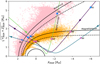 |
Fig. 5 Location of the magnetospheric frontiers crossed by BepiColombo during its three first Mercury flybys. Pink (orange) dots show all BS (MP) crossings identified from MESSENGER and Mariner-10 observations. The solid black, blue, and green lines with arrows show the trajectories of BepiColombo during MFB1, MFB2, and MFB3, respectively, together with the outbound BS (blue crosses) and inbound and outbound MP (pink crosses) crossings identified by MEA and MPPE. The two solid conic lines correspond to average BS and MP locations derived from MESSENGER observations, whereas the two dashed conic lines correspond to the fit to the outbound boundary locations identified by MEA and MPPE. |
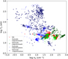 |
Fig. 6 Map of the different regions crossed during the three flybys of Mercury by BepiColombo, in the density and temperature space. The dark blue squares, light blue diamonds, dark green crosses, light green plus signs, and red points represent the dawnside and duskside magnetosphere, the dawnside and duskside magnetosheath, and the SW regions, respectively. |
6 Conclusions
The MEA electron observations of different SW properties encountered during the first three Mercury flybys reveal the highly dynamic response and variability of the SW-magnetosphere interactions at Mercury. The magnetosphere of Mercury is compressed during MFB1, close to its average state during MFB2, and highly compressed during MFB3.
The MEA electron observations reveal the presence of a wake effect very close behind Mercury when BepiColombo entered the shadow region, a significant dusk-dawn asymmetry in electron fluxes on the nightside magnetosphere, and strongly fluctuating electrons with energies above 100s eV on the dawn-side magnetosphere. Magnetospheric electron densities and temperatures are in the range of 10–30 cm−3 and above a few 100s eV in the pre-midnight-sector, and in the range of 1–100 cm−3 and well below 100 eV in the post-midnight sector, respectively. A good match is found between the electron plasma parameters derived by MEA in the various regions of the Hermean environment and similar ones derived in a few cases from other instruments on board BepiColombo. The density-temperature map of electron populations at Mercury illustrates the properties of the different regions of Mercury’s magnetosphere crossed during the BepiColombo flybys.
Acknowledgements
The authors acknowledge all members of the BepiColombo mission for their unstinted efforts in making the missions successful. In particular the MEA Team would like to thank Claude Aoustin for managing the technical activities of the instrument development at IRAP. French co-authors acknowledge the support of Centre National d’Etudes Spatiales (CNES, France) to the BepiColombo mission. BepiColombo is a joint space mission between the European Space Agency (ESA) and the Japan Aerospace Exploration Agency (JAXA). MPPE is funded by JAXA, CNES, the Centre National de la Recherche scientifique (CNRS, France), the Italian Space Agency (ASI), and the Swedish National Space Agency (SNSA). At the start of this work M.R. was funded by a CNES postdoctoral fellowship and is now funded by the European Union’s Horizon 2020 program under grant agreement No 871149 for Europlanet 2024 RI. S.A. was supported by JSPS KAKENHI number 22J01606. M.F. and N.K. are supported by the German Space Agency DLR under grant 50QW2101. Open research section: The metakernel file used to derive BepiColombo’s trajectories and MEA electron parameters displayed here are available for download at https://zenodo.org/records/10911219. The Mariner 10 plasma data used here are available from NASA’s Planetary Data System here for the plasma moments (https://doi.org/10.17189/1519735) and here for the counts (https://doi.org/10.17189/1519734). The BepiColombo and Mariner 10 spice kernels used to determine the times of the entry into or exit from the eclipse region are available at https://doi.org/10.5270/esa-dwuc9bs and https://naif.jpl.nasa.gov/pub/naif/M10/kernels/, respectively.
Appendix A Derivation of electron parameters from MEA1 observations
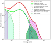 |
Fig. A.1 Count rate |
In order to help the reader to understand how ne and Te were derived, we set out here the method described in Rojo et al. (2023). The procedure is summarized in Figure A.1. We proceeded in four steps using 3D data products of MEA1: (1) we detected the maximum count rate (solid red line) associated with the electron core population. Assuming it to be isotropic and Maxwelllian, we fit the electron core with a Maxwellian distribution function (red stars). (2) We subtracted the fit from the original count rate signal. The results include a low (uniform shaded purple area) and a high-energy (hatched shaded purple area) residual count rate. The low-energy residual was associated with secondary emission and was then removed. (3) We summed the Maxwellian fit representing the electron core population with the high-energy residual count rate to obtain a new count rate signal without secondary electrons (dashed dark brown line). (4) We deduced ne and Te from the resulting new count rate signal by integrating it with Equations 4 and 5 from Rojo et al. (2023).
When BepiColombo is close enough to the Sun (rBepi–Sun < 0.4AU), we can detect the maximum count rate of the core electron population from OMNI data products. This peak can only be detected in the MEA1 sectors open to space. Hence, applying the same procedure to the OMNI count rate (solid green line), we should retrieve the same value of Te. On the other hand, estimates of ne from OMNI data products should be underestimated. We present in Fig. A.2a and A.2b a comparison between the densities and temperatures estimated from 3D and OMNI data, respectively. In these figures we use MEA1 data obtained inside 0.4 AU during the three Mercury flybys and the SW October 2022 campaign. We see that Te and ne calculated from 3D and OMNI data are highly correlated, with a correlation coefficient, r, of 0.92 for each moment and Te,3D ≈ 1.1 × Te,OMNI, which confirms our hypothesis. The electron densities calculated from OMNI data can be multiplied by a constant factor to reproduce the density calculated from 3D data. With this method, the secondary low-energy electrons included in the OMNI data of MEA1 are efficiently removed.
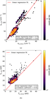 |
Fig. A.2 Correlations between electron moments derived with 3D and Omni data product: (a) Comparison between density and (b) temperatures. |
Appendix B Estimation of the uncertainties on electron parameters
With the current configuration of BepiColombo, it is difficult to accurately estimate the uncertainties due to several issues. (1) The MEA is located in a tiny space at the bottom of MOSIF. Spacecraft charging inside the MOSIF thermal shield can prevent low-energy electrons from entering MEA1. This charging effect depends on SW parameters that are time-variable. (2) The narrow FoV of MEA1 forces us to make the assumption that the electron populations are isotropic, which is not always true. (3) The electron densities are first determined using the 3D data products from MEA1, then a correction is applied to the electron density determined from the OMNI data products, assuming that the two densities are correlated.
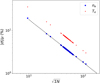 |
Fig. B.1 Relative variation (|σ/µ|) of density (blue) and temperature (red) as a function, |


We estimated the systematic uncertainties on the plasma parameters by using Equations 2 and 19 in the article of Gersh-man et al. (2015). We calculated the parameter uncertainties from velocity distribution functions with random errors, using 3D data products from MEA1. The relative uncertainties of ne and Te are shown in Figure B.1. Here, N represents the counts of an entire distribution, and σ and µ are the uncertainty and the parameter value (here ne or Te), respectively. We find that the relative uncertainties of the density, δne, lie between 1% and 20% and that the relative uncertainties of the temperature, δTe, lie between 3% and 35%. The median values of δne and δTe are 3.7% and 7%, respectively. Because of all the error sources discussed above, we estimate that those uncertainties can only represent lower limits. Moreover, the fact that the density and temperature errors scale almost perfectly as  is due to the Maxwellian fit on the core electron population. We decided not to show the error bars in Figure 3 and 4 because, due to the use of a logarithmic scale, the error bars would not be visible.
References
- Aizawa, S., Harada, Y., Andre, N., et al. 2023, Nat. Commun., 14, 4019 [NASA ADS] [CrossRef] [Google Scholar]
- Aizawa, S., Rojo, M., André, N., et al. 2024, Nature, submitted [Google Scholar]
- Alberti, T., Sun, W., Varsani, A., et al. 2023, A&A, 669, A35 [NASA ADS] [CrossRef] [EDP Sciences] [Google Scholar]
- Dakeyo, J.-B., Maksimovic, M., Démoulin, P., Halekas, J., & Stevens, M. L. 2022, ApJ, 940, 130 [NASA ADS] [CrossRef] [Google Scholar]
- Geach, J., Schwartz, S., Génot, V., et al. 2005 in, Copernicus Publications Göttingen, Germany, 931 [Google Scholar]
- Gershman, D. J., Dorelli, J. C., F.-Viñas, A., & Pollock, C. J. 2015, J. Geophys. Res.: Space Phys., 120, 6633 [CrossRef] [Google Scholar]
- Griton, L., Issautier, K., Moncuquet, M., et al. 2023, A&A, 670, A174 [NASA ADS] [CrossRef] [EDP Sciences] [Google Scholar]
- Hadid, L., Delccourt, D., Harada, Y., et al. 2024, Nat. Commun., submitted [Google Scholar]
- Halekas, J., Angelopoulos, V., Sibeck, D., et al. 2014, The ARTEMIS Mission, 93 [Google Scholar]
- Harada, Y., Aizawa, S., Saito, Y., et al. 2022, Geophys. Res. Lett., 49, e2022GL100279 [CrossRef] [Google Scholar]
- Jia, X., Slavin, J. A., Poh, G., et al. 2019, J. Geophys. Res.: Space Phys., 124, 229 [NASA ADS] [CrossRef] [Google Scholar]
- Kasaba, Y., Kojima, H., Moncuquet, M., et al. 2020, Space Sci. Rev., 216, 1 [CrossRef] [Google Scholar]
- Korth, H., Johnson, C. L., Philpott, L., Tsyganenko, N. A., & Anderson, B. J. 2017, Geophys. Res. Lett., 44, 10 [NASA ADS] [CrossRef] [Google Scholar]
- Lavraud, B., Fargette, N., Réville, V., et al. 2020, ApJ 894, L19 [Google Scholar]
- Murakami, G., Hayakawa, H., Ogawa, H., et al. 2020, Space Sci. Rev., 216, 1 [CrossRef] [Google Scholar]
- Ogilvie, K., Scudder, J., Hartle, R., et al. 1974, Science, 185, 145 [NASA ADS] [CrossRef] [Google Scholar]
- Ogilvie, K., Scudder, J., Vasyliunas, V., Hartle, R., & Siscoe, G. 1977, J. Geophys. Res., 82, 1807 [NASA ADS] [CrossRef] [Google Scholar]
- Rojo, M., Persson, M., Sauvaud, J.-A., et al. 2023, A&A, in press [Google Scholar]
- Saito, Y., Delcourt, D., Hirahara, M., et al. 2021, Space Sci. Rev., 217, 1 [NASA ADS] [CrossRef] [Google Scholar]
- Sun, W., Dewey, R. M., Aizawa, S., et al. 2022, Sci. China Earth Sci., 1 [Google Scholar]
- Tao, J., Ergun, R., Newman, D., et al. 2012, J. Geophys. Res.: Space Phys., 117, A03106 [Google Scholar]
- Whittlesey, P. L., Larson, D. E., Kasper, J. C., et al. 2020, ApJS, 246, 74 [Google Scholar]
- Xu, X., Xu, Q., Chang, Q., et al. 2019, ApJ, 881, 76 [NASA ADS] [CrossRef] [Google Scholar]
- Zhao, J.-T., Zong, Q.-G., Slavin, J., et al. 2020, Geophys. Res. Lett., 47, e88075 [NASA ADS] [Google Scholar]
All Tables
Time (in UTC) of the different boundary crossings identified from electron observations during MFB1 (October 1, 2021), MFB2 (June 23, 2022), MFB3 (June 19, 2023), and M10 FB1 (March 29, 1974).
Estimated distance of extrapolated standoff BS and MP locations, estimated SW dynamic pressure (in nPa), SW density derived from MEA observations (in cm−3) at the BS in the SW, and estimated SW velocity (in km s−1), for inbound and outbound observations.
All Figures
|
Fig. 1 Geometry of the flybys from BepiColombo and Mariner 10 in the MSO coordinate system with average BS and MP models displayed with dashed gray lines. The origin of the MSO coordinate system is at the planetary center of mass, +X is sunward, +Y lies in the orbital plane, perpendicular to +X and opposite to the direction of planetary orbital motion (i.e., +Y is positive toward dusk), and +Z is normal to the orbital plane and positive northward. From left to right: MFB1 (October 1, 2021), MFB2 (June 23, 2022), MFB3 (June 19, 2023), and M10 FB1 (March 29, 1974). Top: trajectories in the XY plane. Bottom: trajectories in the XZ plane. Distances to the planet are given in Mercury radii, 1 RM = 2440 km. The marks are the time in UTC (HH:MM). |
| In the text | |
|
Fig. 2 Energy-distance spectrograms of electron count rates displayed as a function of the distance along the YMSO axis. From top to bottom: MEA1 observations for MFB1, MFB2, and MFB3, and SES observations for M10 FB1. The vertical dashed green line delineates the CA. For each flyby, the spacecraft altitude (in Mercury radius) and the time (in UTC, HH:MM) are indicated below the corresponding plot. We note that the time increases from right to left. The red, green, and light and dark blue boxes above the corresponding plot delineate the SW, the magnetosheath, the magnetosphere, and the eclipse (or shadow regions) crossed by the spacecraft for each flyby, respectively. |
| In the text | |
|
Fig. 3 Electron density measured during BepiColombo and Mariner 10 flybys. From top to bottom: electron density profiles for MFB1, MFB2, MFB3, and M10 FB1 displayed as a function of the distance along the YMSO axis. The vertical dashed green line delineates the CA. For each flyby, the spacecraft altitude (in Mercury radius) and the time (in UTC, HH:MM) are indicated below the corresponding plot. We note that the time increases from right to left. The red, green, and light and dark blue boxes below the corresponding plot delineate the SW, the magnetosheath, the magnetosphere, and the eclipse or shadow regions crossed by the spacecraft for each flyby, respectively. The blue stars and red crosses represent the densities deduced from the 3D and OMNI data products of MEA1, respectively. |
| In the text | |
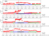 |
Fig. 4 Same as Fig. 3 but for the temperature of electrons (in eV). |
| In the text | |
|
Fig. 5 Location of the magnetospheric frontiers crossed by BepiColombo during its three first Mercury flybys. Pink (orange) dots show all BS (MP) crossings identified from MESSENGER and Mariner-10 observations. The solid black, blue, and green lines with arrows show the trajectories of BepiColombo during MFB1, MFB2, and MFB3, respectively, together with the outbound BS (blue crosses) and inbound and outbound MP (pink crosses) crossings identified by MEA and MPPE. The two solid conic lines correspond to average BS and MP locations derived from MESSENGER observations, whereas the two dashed conic lines correspond to the fit to the outbound boundary locations identified by MEA and MPPE. |
| In the text | |
|
Fig. 6 Map of the different regions crossed during the three flybys of Mercury by BepiColombo, in the density and temperature space. The dark blue squares, light blue diamonds, dark green crosses, light green plus signs, and red points represent the dawnside and duskside magnetosphere, the dawnside and duskside magnetosheath, and the SW regions, respectively. |
| In the text | |
|
Fig. A.1 Count rate |
| In the text | |
|
Fig. A.2 Correlations between electron moments derived with 3D and Omni data product: (a) Comparison between density and (b) temperatures. |
| In the text | |
|
Fig. B.1 Relative variation (|σ/µ|) of density (blue) and temperature (red) as a function, |
| In the text | |
Current usage metrics show cumulative count of Article Views (full-text article views including HTML views, PDF and ePub downloads, according to the available data) and Abstracts Views on Vision4Press platform.
Data correspond to usage on the plateform after 2015. The current usage metrics is available 48-96 hours after online publication and is updated daily on week days.
Initial download of the metrics may take a while.