| Issue |
A&A
Volume 679, November 2023
|
|
|---|---|---|
| Article Number | A43 | |
| Number of page(s) | 12 | |
| Section | Extragalactic astronomy | |
| DOI | https://doi.org/10.1051/0004-6361/202347430 | |
| Published online | 01 November 2023 | |
Time-dependent photoionization spectroscopy of the Seyfert galaxy NGC 3783
1
SRON Netherlands Institute for Space Research, Niels Bohrweg 4, 2333 CA Leiden, The Netherlands
e-mail: This email address is being protected from spambots. You need JavaScript enabled to view it.
2
RIKEN High Energy Astrophysics Laboratory, 2-1 Hirosawa, Wako, Saitama 351-0198, Japan
3
Leiden Observatory, Leiden University, PO Box 9513 2300 RA Leiden, The Netherlands
4
MIT Kavli Institute for Astrophysics and Space Research, Massachusetts Institute of Technology, Cambridge, MA 02139, USA
5
Space Telescope Science Institute, 3700 San Martin Drive, Baltimore, MD 21218, USA
6
Anton Pannekoek Institute, University of Amsterdam, Postbus 94249, 1090 GE Amsterdam, The Netherlands
Received:
11
July
2023
Accepted:
9
September
2023
Abstract
We present an investigation into the spectroscopic properties of non-equilibrium photoionization processes operating in a time-evolving mode. Through a quantitative comparison between equilibrium and time-evolving models, we find that the time-evolving model exhibits a broader distribution of charge states, accompanied by a slight shift in the peak ionization state depending on the source variability and gas density. The time-evolving code tpho in SPEX was successfully employed to analyze the spectral properties of warm absorbers in the Seyfert galaxy NGC 3783. The incorporation of variability in the tpho model improves the fits of the time-integrated spectra, providing more accurate descriptions of the average charge states of several elements, in particular Fe, which is peaked around Fe XIX. The inferred densities and distances of the relevant X-ray absorber components are estimated to be approximately a few times 1011 m−3 and ≤1 pc, respectively. Furthermore, the updated fit suggests a potential scenario in which the observed absorbers are being expelled from the central active galactic nucleus at the escape velocities. This implies that these absorbers might not play a significant role in the active galactic nucleus feedback mechanism.
Key words: X-rays: galaxies / galaxies: active / galaxies: Seyfert / galaxies: individual: NGC 3783
© The Authors 2023
 Open Access article, published by EDP Sciences, under the terms of the Creative Commons Attribution License (https://creativecommons.org/licenses/by/4.0), which permits unrestricted use, distribution, and reproduction in any medium, provided the original work is properly cited.
This article is published in open access under the Subscribe to Open model. This email address is being protected from spambots. You need JavaScript enabled to view it. to support open access publication.
1. Introduction
Warm absorbers are one of the manifestations of photoionized outflows from active galactic nuclei (AGNs). Within the X-ray regime, they are often recognized as absorption features characterized by a diverse range of ionization states. These features typically exhibit hydrogen column densities ranging from 1024 to 1026 m−2 and outflow velocities of approximately ∼100 − 1000 km s−1 (Reynolds 1997; Blustin et al. 2005; Kaastra et al. 2012; Laha et al. 2021). While warm absorbers have been extensively observed and studied, two outstanding questions remain regarding the interpretation of these observations: (1) whether the conventional practice of modeling absorbers as discrete ionization components, each in photoionization equilibrium, is a reasonable approximation; and (2) the precise locations and mechanisms responsible for launching these outflows.
For warm absorbers, the development of photoionization equilibrium with an external ionizing source requires a certain timescale, which is commonly approximated by the recombination time of the absorbers (Krolik & Kriss 1995; Nicastro et al. 1999). To maintain steady equilibrium, it is crucial for the recombination time to be considerably shorter than the characteristic variation time of the ionizing source. This condition ensures that the system can promptly and effectively respond to fluctuations in the intensity of the ionizing radiation. However, it is not guaranteed that all warm absorbers satisfy this condition. The recombination time depends on various factors, including the electron density and ionization state, and with the current limited knowledge of absorber density (e.g., Gabel et al. 2005; Arav et al. 2015), the recombination time could range from 104 to 108 s. On the other hand, power spectral analysis conducted by Uttley et al. (2002) and Markowitz et al. (2003) has shown that a significant portion of X-ray variations occur on timescales of 105–107 s. When the two timescales become comparable, warm absorbers are unable to achieve equilibrium, resulting in the variations in their ionization states lagging behind the intrinsic variations in the AGNs (e.g., Silva et al. 2016).
To address the nonequilibrium photoionization condition, several time-evolving photoionization codes that build upon existing equilibrium models have recently been developed: CLOUDY (van Hoof et al. 2020), XSTAR (Sadaula et al. 2023), TEPID (Luminari et al. 2023), and SPEX (Rogantini et al. 2022). These codes incorporate ionizing light curves and spectral energy distributions (SEDs) and self-consistently solve the time-dependent equations governing the ionization and thermal states as a function of gas density. By employing such time-evolving models, a more accurate approximation of the true state of warm absorbers can be obtained, which resolves question (1). Furthermore, these models have the potential to provide insights into question (2), namely the determination of the distances at which the warm absorbers are located. The distance can be constrained using the relation  , where L represents the ionizing luminosity, nH denotes the hydrogen number density, and ξ is the ionization parameter. The time-evolving calculations are able to incorporate all three parameters, whereas in equilibrium modeling it becomes challenging to constrain the gas density accurately (Kaastra et al. 2004, 2012).
A significant portion of past work has focused on density diagnostics, utilizing response lags (Nicastro et al. 1999; Silva et al. 2016; Juráňová et al. 2022; Rogantini et al. 2022; Li et al. 2023) and absorption line features from metastable levels (Kaastra et al. 2004; Gabel et al. 2005; Edmonds et al. 2011; Di Gesu et al. 2013; Mehdipour et al. 2017). However, there is only limited knowledge about the overall characteristic spectroscopic features specific to time-evolving photoionized plasmas (Rogantini et al. 2022). Acquiring such knowledge would be beneficial in two aspects: firstly, it would provide a systematic understanding of the practical differences between equilibrium and time-evolving models; secondly, it would allow us to explore the potential to constrain the density and distance of the observed warm absorbers through direct spectral analysis. In this work we aim to characterize the time-evolving spectral model by differentiating it from the equilibrium model and apply it to real warm absorber observations. We utilized the SPEX tpho (Rogantini et al. 2022) and pion (Mehdipour et al. 2016) models as the baseline for the time-dependent and equilibrium conditions, respectively.
The time-dependent photoionization model was applied to existing data of the Seyfert 1 galaxy NGC 3783 (z = 0.009730, Theureau et al. 1998). This AGN is well known for its prominent warm absorber, characterized by narrow absorption lines originating from various elements, including Fe, Ca, Ar, S, Si, Al, Mg, Ne, O, N, and C. The observed absorption lines span a wide range of ionization states, with a total column density of ∼4 × 1026 m−2. Previous studies have reported an average outflow velocity of approximately 600 km s−1 for this warm absorber (Kaspi et al. 2000, 2001, 2002; Scott et al. 2014). The X-ray absorption spectra have been modeled using different approaches, incorporating two ionized components (Blustin et al. 2002; Krongold et al. 2003, 2005), three components (Netzer et al. 2003), five components (Ballhausen et al. 2023), nine components (Mehdipour et al. 2017; Mao et al. 2019; Kaastra et al. 2018), or a broad continuous absorption measure distribution (Gonçalves et al. 2006; Behar 2009; Goosmann et al. 2016; Keshet & Behar 2022). All existing models assume photoionization equilibrium.
The structure of the paper is as follows. In Sect. 2 we present a theoretical exploration of the spectroscopic characteristics of the tpho model. In Sect. 3 we employ the tpho model to analyze the Chandra grating data of NGC 3783. Finally, the findings are discussed and summarized in Sect. 4. Throughout the paper, the errors are given at a 68% confidence level.
2. Time-dependent photoionization model
In order to investigate the general spectral characteristics of a time-varying photoionized source, we performed a series of time-dependent calculations using the SPEX tpho routine (Rogantini et al. 2022) and the NGC 3783 ionized outflow configuration as described in Mehdipour et al. (2017) and Mao et al. (2019). By utilizing the eigenvector method initially described in Kaastra & Jansen (1993), the tpho model self-consistently calculates the out-of-equilibrium time evolution of photoionization, accurately determining the ion concentrations and electron temperature of the ionized source as a function of time. One advantage of the tpho model, as highlighted in Rogantini et al. (2022) and Li et al. (2023), is its potential as a density diagnostic tool for the target source. The recombination process, influenced by collisional interactions, is directly linked to the electron density of the source.
The ionizing SED and its corresponding light curve, as well as the NGC 3783 warm absorber outflows, have been modeled in accordance with the methods outlined in Li et al. (2023). The SED comes originally from the time-averaged spectral analysis of the optical to hard X-ray data in its unobscured phase during 2000–2001. As described in Mehdipour et al. (2017), the archival data from Hubble Space Telescope, Chandra, XMM-Newton, and NuSTAR were fit jointly to determine the SED. The light curve is derived by a simulation based on the power spectrum obtained from a large set of XMM-Newton and Rossi X-ray Timing Explorer (RXTE) data (Markowitz 2005). Li et al. (2023) demonstrate that a simulated light curve spanning approximately 1 × 10⁷ s is adequate for capturing the primary variability that occurs within the range 105–106 s. The fractional variability of the model light curve, defined as the ratio of the standard deviation to the average flux, is approximately 40%. The warm absorbers in the target are taken from the results of Mehdipour et al. (2017) and Mao et al. (2019) using data from the Chandra and XMM-Newton gratings, which revealed nine distinct photoionization components with the ionization parameter log ξ spanning a range from −0.65 to 3 (see Table 3 in Mao et al. 2019 and Table 1).
pion constraints on the warm absorber properties.
2.1. Effects on ion concentration
To characterize the effect on ion concentration for a time-averaged absorption spectrum, we performed a full tpho run based on a simulated light curve, which enabled us to track the time-dependent evolution of ion concentration throughout the period of interest. A weighting factor based on the square root of the X-ray flux was applied to determine the mean ion concentration for a time-integrated spectrum. The gas densities of the nine warm absorber components were set to vary between 108 m−3 and 1015 m−3. To make sure that the results are statistically robust, each simulation was conducted for a considerable duration of ∼5 × 10⁷ s as shown in Fig. 1. With the tpho model it is assumed that the ionizing SED retains its shape over the period.
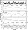 |
Fig. 1. Simulated light curve (upper panel) and the corresponding evolution of the average Fe charge of component 3 (lower panels). The average charge variations are shown as solid lines for gas densities of 1014, 1012, 1010, and 108 m−3, while the dashed curves illustrate the corresponding source light curves in the same period. As the gas density decreases, the response time to source variations becomes longer, resulting in flatter average charge variations. To highlight the response time differences across various densities, each panel presents a different total time period. |
First we examined how the ionization state of the individual warm absorber component changes over time. Figure 1 provides a visual representation of the temporal evolution of the Fe average charge of component 3 (Table 1) in the warm absorber. The average charge CFe was computed as  , where c(Fei+) represents the concentration of Fe ions with a charge i. Component 3 was chosen as it encompasses a wide span of Fe ion species given its log ξ of 2.55 (Mao et al. 2019), providing a clear visualization of the potential changes. The average charge exhibits a minor delay of ≤104 s with respect to the light curve for a gas density of around 1014 m−3. As the gas density decreases, the amplitude of the charge variation decreases while the delay between the light curve and the average charge evolution increases. The underlying density-delay relation presented in this figure is consistent with those reported in previous studies on time-dependent evolution of warm absorber states (Juráňová et al. 2022; Rogantini et al. 2022; Li et al. 2023).
In Fig. 2 we plot the mean ion concentrations of Fe with three different gas densities for the warm absorber component 3. At low density, the ion concentration can be well reproduced by a single equilibrium pion component, indicating a stable state where the effect on ion concentration by a changing SED is minimal. While for a high density cloud, the obtained mean ion concentration needs to be approximated by two equilibrium components with distinct ionization parameters. Furthermore, the normalizations of the two equilibrium components tend to converge at high densities. This behavior arises from two factors. Firstly, for a fixed ionization parameter and SED, the product of density and distance from the source remains constant. As the density increases, the distance from the source decreases, leading to a higher ionizing flux. At the same time, the rate of recombination due to collisions scales with density in the same way. These factors together result in a larger fluctuation in the ion concentration and a broader mean charge distribution at high densities.
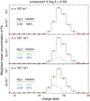 |
Fig. 2. Average concentration distributions of Fe ions obtained from simulation runs with gas densities of 108, 1011, and 1014 m−3 for component 3. The obtained ion concentrations are shown as red dots. The best-fit total concentration, depicted as black lines, is the sum of the two equilibrium components depicted as blue and green lines. The ionization parameters and the fractional contributions of the two equilibrium components are also shown. A single component is sufficient to fit the average concentration in the case of 108 m−3. |
Here we conducted a systematic comparison between time-evolving and equilibrium spectra. For each warm absorber component, a single pion distribution was utilized to fit the simulated tpho ion concentration of Fe. This fitting process allowed us to determine the deviation of log ξ from its original value, for example, log ξ = 2.55 for component 3. To quantify the overall effect, we calculated the average log ξ deviations by taking the mean across all nine components. We note that this approach would, however, overlook the potential differences between the high and low ionization components (e.g., Juráňová et al. 2022). As shown in Fig. 3, the log ξ deviations are negligible at low densities when the cloud maintains an approximately “stable” state throughout the simulation with a recombination timescale of ∼1010 s, which is longer than the entire simulation duration. However, as the density increases, the pion-measured log ξ tends to underestimate the intrinsic value by approximately 0.05 at a density of 1013 − 1014 m−3, given a typical light curve fractional variability of ∼40%. The deviation of log ξ becomes small again once the density reaches 1015 m−3, as the cloud recombination timescale decreases to ≤103 s, making it considerably shorter than the light curve variability timescale. On the other hand, at high densities, the oscillation of the ionization state results in a more even distribution of charge states. Figure 3 demonstrates that for a cloud density of 1014 m−3, the dispersion in ion concentration σFe is 40% higher than that predicted by the equilibrium solution, assuming a light curve fractional variability of approximately 40%. Therefore, it can be inferred that the ionization parameter may be underestimated by the equilibrium solution in situations where the plasma is in a “delayed” state (Rogantini et al. 2022; Li et al. 2023) where recombination takes place at a timescale that is comparable to the light curve variability. In situations where the timescale of recombination is much longer (“stable”) or shorter (“equilibrium”) than the timescale of source variation, the central ionization parameters obtained in equilibrium would be less biased, although the ion concentration becomes significantly more dispersed than a single pion component in the “equilibrium” scenario as also illustrated in Fig. 2.
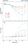 |
Fig. 3. Deviation of log ξ (a) and the dispersion of the Fe ion concentration (b) plotted as a function of gas densities for light curves with fractional variability ranging from 10% to 50% (the simulated light curve shown in Fig. 1 has an average fractional variability, Fvar, of ∼40%). The deviation of log ξ is calculated as the difference between the intrinsic value and the value obtained from a single equilibrium component fitting of the simulated Fe ion concentration distribution, such as the ones shown in Fig. 2. The curves representing the averages over the nine warm absorber components (see Table 1) are plotted for both the deviation and dispersion. |
In Fig. 4 we present the accumulated ionic column densities of Fe as a function of gas density throughout the simulated period. These column densities are obtained by summing the contributions from the nine warm absorber components in NGC 3783. In this calculation, all components are assumed to have the same density. The results reveal that, for a gas density of 108 m−3, the ionic column density closely aligns with the pion model assuming ionization and thermal equilibrium. However, at a higher gas density of 1014 m−3, the curve deviates significantly from the pion solution, particularly at the peaks corresponding to Fe XIX and Fe XXV. Moreover, the tpho curve exhibits a slightly larger concentration of low ionization species (Fe VIII to Fe XV) compared to the pion case. This discrepancy can be, at least partly, attributed to the dispersion effect in ion concentration (as shown in Fig. 3b) caused by the decreasing recombination timescale. These results demonstrate the potential of absorption spectroscopy using a proper time-dependent model to offer useful constraints on gas density.
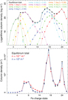 |
Fig. 4. Column densities of Fe in equilibrium and the time-evolving condition. The upper panel shows the total column density of Fe in equilibrium, with each individual component plotted in a different color. To capture the wide range of concentrations, which span several orders of magnitude, a logarithmic scale is employed. The lower panel compares the equilibrium column density (represented as a dashed black line) to the average column density of time-dependent photoionization, with gas densities of 108 and 1014 m−3 shown as blue and red lines. |
3. Application to the 2000 and 2001 Chandra/HETGS observations
In order to investigate the feasibility of our approach on actual observations, we performed a self-consistent tpho modeling on the Chandra High Energy Transmission Grating Spectrometer (HETGS) data obtained during the unobscured period of 2000–2001 (Table 2). We limited our analysis to a relatively small set of data as the current tpho model still requires a significant amount of computational resources, which prevented us from extending our analysis to data of other time periods or instruments. To process the data, we utilized the CIAO v4.15 software and calibration database (CALDB) v4.10. The chandra_repro script was used to perform data screening and generate spectral files for each exposure. We then merged the spectra for orders ±1 using the CIAO combine_grating_spectra tool, along with the associated response files. We performed a joint fit on the medium energy grating spectrum, which covers the wavelength range 6 − 16.5 Å, and the high energy grating spectrum in the 1.8 − 3.1 Å range.
NGC 3783 Chandra HETGS data.
Figure 5 depicts the RXTE and HETGS light curves of NGC 3783 from July 1999 to December 2001. To perform the time-dependent calculation for each Chandra observation, we utilized the HETGS light curve in combination with the RXTE light curve obtained prior to the Chandra observation. By incorporating the RXTE light curve, we were able to track the changes in the source and model the possible delayed response in the ionization state, which can potentially have an impact on the HETGS data. The PIMMS tool was used to convert the RXTE count rate to the HETGS rate based on the broadband spectral model described in Sect. 3.1. As shown in Fig. 5, during a few overlapping periods of the two instruments, the converted RXTE count rates match the HETGS rates well. Due to the limited coverage of the RXTE data for observations 1, 5, and 6, the short-term variability is not well captured, possibly introducing a systematic bias. Further details regarding this uncertainty will be discussed in Sect. 3.2.
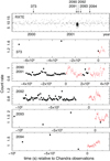 |
Fig. 5. RXTE and Chandra HETGS light curves of NGC 3783 from mid-1999 to the end of 2001. The upper panel shows the RXTE proportional counter array data in the 2 − 60 keV band, with the average flux level indicated by a horizontal line. The Chandra HETGS light curves are presented in the panels below as red data points, along with the adjacent RXTE data converted using the PIMMS tool. |
Using the method outlined in Uttley et al. (2002) and Markowitz (2005), we computed the combined power spectrum for the RXTE and Chandra data taken between July 1999 and December 2001. Figure 6 shows that the resulting spectrum agrees well with the doubly broken model presented in Markowitz (2005), which was also utilized to generate the light curve used in Sect. 2. This agreement indicates that the variability observed during the Chandra observations aligns well with the average properties of this AGN. Considering that the primary variability of the source arises from variations detected by RXTE below the break frequency of 4 × 10⁻⁶ Hz, the Chandra exposures would capture mostly the tail end of the variability on shorter timescales.
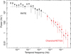 |
Fig. 6. Power spectral density function of the combined RXTE (black) and Chandra HETGS (red) light curves shown in Fig. 5. The data are compared with the model (dashed line) based on the best-fit results obtained in Markowitz (2005) on the data in the 0.2 − 12.0 keV range. |
3.1. Spectral analysis
For each HETGS exposure, we fit one time-integrated spectrum by utilizing a time-evolving scheme as follows. By adopting the approach presented in Mehdipour et al. (2017), Kaastra et al. (2018), and Mao et al. (2019), we first built up a contemporaneous SED that serves as the photoionization continuum for the pion and tpho components. This continuum model includes a Comptonized disk component (comt), a power-law with cut-off (pow), and a neutral reflection component (refl). Together, these components form the intrinsic SED. We allowed the normalizations of the three continuum components to vary between different pointings to account for the intrinsic variability of the nucleus as indicated in the light curve. To model the warm absorbers, we used a total of nine quiescent pion absorption components, whose column densities, ionization parameters, outflow, and microscopic turbulence velocities are fixed to those obtained in Mao et al. (2019). For the photoionized emission, we used three pion components with positive covering relative to the nucleus, two for the X-ray narrow emission feature and one for the broad features. The properties of these emission pion components are also set to the values determined in Mao et al. (2019). By fitting the global spectrum, we determined the contemporaneous SED for each HETGS pointing.
We further explored the modeling of the warm absorber components using the pion model. For warm absorber components 1 to 5, we allowed the column densities and ionization parameters to vary, while keeping the outflow and microscopic turbulence velocities consistent with the values from Mao et al. (2019). To account for variations in the ionization parameter across different observations, we assumed that the hydrogen densities and distances of the warm absorbers remain constant. As a result, the ionization parameter for each observation is scaled by the contemporaneous SED obtained above in the 1 − 103 Ryd range. Due to the limited constraining power of the HETGS data on components at low ionization states, we chose to fix the column densities and ionization parameters of components 6–9 to the values reported in Mao et al. (2019). We assumed that each pion component extends significantly along the line of sight, with a covering factor of 1. The results obtained from the pion fit can be found in Table 1.
We proceeded by replacing the nine pion absorption components with corresponding tpho components. These tpho components calculate the time-dependent spectrum based on the obtained light curves and contemporaneous SEDs. In the tpho modeling, both the Chandra and adjacent RXTE light curves (Fig. 5) are utilized, while the output model represents the integrated spectrum within the Chandra period. Therefore, the fitting results provide an average characterization of the properties observed during the Chandra observations. The basic setup of the tpho components remains identical to that of the pion components, except for one key difference: the hydrogen number densities are allowed to vary freely in the tpho modeling of warm absorber components 1–5. This variation in hydrogen number densities enables the modeling of time-dependent behavior within these components, contrasting with the pion modeling where the densities are not constrained. For the low ionization components 6–9, the column densities and ionization parameters are fixed to the values reported in Mao et al. (2019). Their hydrogen number densities are set to their lower limits, effectively turning off their time evolution. The tpho results are summarized in Table 3.
tpho and UV constraints on the physical properties of the warm absorbers.
The fit that utilizes the tpho component results in a C-statistic of 12 116 for an expected value of 8073, which is a mild improvement over the C-statistic of 12 889 obtained with the pion model. In order to gain insight into the enhanced modeling of the spectral features by tpho, we conducted an analysis employing the slab model. This model allowed us to independently determine the column density of each ionic species, without relying on assumptions regarding the ionization balance. Thereby, the slab component can be considered as a complete, independent representation of the ionization state of the warm absorbers. To mitigate the level of degeneracy, we employed two slab components, instead of nine, to model the absorption feature for each HETGS observation. The first component was introduced with a velocity varying in the range −400 to −600 km s−1, representing warm absorber components 1, 4, and 5. The second slab component encompasses an outflow velocity ranging from −800 to −1600 km s−1 and combines warm absorber components 2, 3, 6, 7, 8, and 9. The turbulence velocities of the two slab components were fitted freely. The fit that utilizes the two slab components yields a satisfactory C-statistic of 11 844 for an expected value of 8058. The addition of a third slab component does not yield any further significant improvement in the fitting quality.
By substituting the nine tpho components with these two slab components, we fit the set of HETGS data again. We permitted the column densities of Fe species from Fe IX to Fe XXVI, Ne ions from Ne III to Ne X, Mg ions from Mg VIII to Mg XII, Si ions from Si X to Si XIV, and S ions from S XI to S XVI to vary freely for both slab components. To reduce degeneracy, we kept the column densities of O, Na, Al, Ar, Ca, and Ni, as well as the remaining species of Ne, Mg, Si, S, and Fe, at the fixed values determined from the global tpho fit. The column densities combining the two slab components can be thus used as the absolute absorption values for each observation.
Figure 7 displays a comparison of the ionic column densities ranging from Fe IX to Fe XXVI obtained from three different models: pion, tpho, and slab, for each HETGS pointing. All data sets exhibit two prominent peaks centered around Fe XIX and Fe XXV, in line with the average model depicted in Fig. 4. While the current HETGS data lack sufficient constraints on the Fe XXV peak, it becomes evident that the tpho model systematically provides a better or, at the very least, comparable fit to the Fe XIX peak. The pion curves tend to slightly overestimate the peak values in observations 2090, 2091, and 2092. For observation 2093, the pion model seems to underestimate the column density of Fe XIX, meanwhile overestimating that of Fe XX. Some of these features can be better reproduced by utilizing the tpho components. Both models perform similarly when compared to the slab results for observations 373 and 2094.
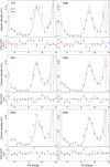 |
Fig. 7. Column densities of all Fe ions ranging from Fe IX to Fe XXVI determined through fitting using the slab model (black data points). The observed data points are compared with the values computed using the pion (red) and tpho (blue) models. Each panel represents one HETGS observation. |
To further compare the results between the slab and the physical models, we computed the average charges of Ne to Fe using the slab fits for each observation. The average charges are plotted in Fig. 8 as a function of the contemporaneous ionizing fluxes, alongside the average charges calculated using the best-fit pion and tpho models. Due to limited constraints, the Mg and S results are not included in the comparison. As the ionizing fluxes increase, we observe a corresponding mild increase in the obtained average charges, indicating for evolving ionization levels under varying ionizing fluxes within a finite recombination time. A similar pattern is found in the total column densities of Fe XIX and Fe XX, which are the predominant iron species. Conducting a statistical comparison among the slab, pion, and tpho results reveals that the tpho model consistently aligns better with the slab results. The pion calculations appear to slightly overestimate the average charges at low ionizing luminosity. This is basically in line with the results depicted in Fig. 7.
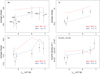 |
Fig. 8. Average charge states of Ne, Si, and Fe, as well as the combined column densities of Fe XIX and Fe XX, plotted as a function of the ionizing luminosity. The average charges are defined in Sect. 2. Each data point corresponds to an individual observation and was obtained via fitting with the slab model. The values obtained from the pion and tpho models are shown with red and blue curves, respectively. The χ-square values between the models and the data are displayed as numbers in the lower-right corner. |
Both the pion and tpho models utilize identical atomic data for calculating ionization balance, thermal balance, and absorption lines. The key distinction lies in the fact that the tpho model introduces time and density dependences in the ionization and thermal states, whereas the pion model adopts equilibrium for both. The better agreement between tpho and slab results thus provides evidence for nonequilibrium states within each observation. This further indicates the presence of nonzero densities for the relevant warm absorption components.
3.2. Systematic uncertainties
An apparent concern with the current tpho approach arises from the combination of RXTE and Chandra light curves, particularly where the RXTE light curves are sparsely sampled in observations 373, 2093, and 2094. Consequently, the RXTE data may not adequately capture the full history of source variations preceding the Chandra observation, potentially introducing systematic biases on the ion concentration variations during the target periods due to the finite recombination time. To estimate the magnitude of this uncertainty, we explored an extreme scenario where each RXTE light curve is transformed into a flat constant at its average value. Consequently, the ion concentration remains constant throughout each RXTE period, resulting in minimal impact on the subsequent variations. By fitting the HETGS data using these modified light curves, we identify fractional differences of ∼5 − 15% in the derived densities of the warm absorber components when compared to the values obtained using the original light curves. Therefore, it is unlikely that the uncertainty in RXTE light curve has substantially affected the current tpho results.
In addition, the assumed equilibrium solution for the initial ionization states of the warm absorber components, obtained from a time-integrated analysis, might introduce bias, as the true condition is likely to be nonequilibrium. Determining the precise initial ionization state presents a challenge in itself. However, we can assess the uncertainty associated with the initial condition by modifying the first data point in the light curve. This would have a significant impact on the evolution of the ionization states since the ionizing flux utilized in the tpho model is a relative value scaled by the first data point in the light curve. To evaluate this uncertainty, we altered the first data point by a fractional change of 15%, determined from the standard deviation of the HETGS light curves averaged over six observations. The modified light curve results in a fractional difference of ∼40 − 80% in the best-fit densities. This suggests that the current assumption regarding the initial ionization state might introduce a substantial systematic uncertainty into the results. The reported density errors in Table 3 and Fig. 9 are derived by combining the statistical errors with the systematic errors stemming from both the RXTE light curve and the initial state.
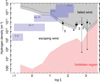 |
Fig. 9. Hydrogen number densities of the warm absorbers plotted as a function of their ionization parameters. Our results for components 1–5 from the tpho model are shown as stars. The gray shaded region represents the region where the outflow is unable to escape the gravitational potential of the black hole due to nH > nesc, while the dashed line indicates the position of |

4. Interpretation and future prospects
4.1. Comparing the time-dependent and equilibrium models
The equilibrium model continues to serve as the current baseline in the examination of photoionized sources, despite some of such sources potentially exhibiting substantial deviations from equilibrium. Consequently, it is crucial to address the similarity and discrepancy between time-dependent and equilibrium models in terms of their spectra. As indicated earlier in Sect. 2, the ion concentrations derived from the equilibrium pion model and the time-dependent tpho model differ in at least two notable aspects: the ionization parameters obtained with pion may exhibit a slight deviation from those with tpho within the density range 1011 − 1015 m−3 in the case of NGC 3783, and tpho tends to yield a broader range of ion species compared to the equilibrial distribution.
As shown in Tables 1 and 3, the ionization parameters derived from the pion model exhibit systematically lower values compared to those obtained using the tpho model, with a difference ranging from 0.05 to 0.1 across various warm absorber components. This aligns well with the expectation illustrated in Fig. 3. Despite the small deviation, it is reasonable to take the warm absorber components identified using the classic pion model in the HETGS band for this object as a valid approximation.
4.2. Constraints on densities and distances of the X-ray absorbers
Although the overall spectral fits with the tpho and pion models yield a marginal difference (C-statistic of 12 116 with tpho and 12 889 with pion), the tpho model shows significant improvements over the pion model in various instances. This is evident in Fig. 8, where the average charge state distributions of Ne, Si, and Fe obtained with the slab significantly favor the tpho model over the pion model. Figure 7 shows that the tpho model consistently better reproduces the ionization peak centered around Fe XIX, primarily originating from warm absorber components 3 and 4 as depicted in Fig. 4. Consequently, this enables us to derive useful constraints on the cloud densities associated with components 3 and 4, while obtaining a more marginal constraint for component 5 at a lower ionization state. However, it should be noted that the current HETGS data only allows for the upper limits to be determined for the densities of components 1 and 2, since these components involve highly ionized Fe where the sensitivity of the present instrument becomes poorer. The obtained density constraints are shown in Fig. 9 and Table 3.
By employing the derived hydrogen number densities, ionization parameters, and source luminosity, we can calculate the distance between the absorber components and the central source. Based on observed densities of several times 1011 m−3, the distances for components 3–5 are obtained to be around 1 − 2 × 10¹⁶ m (0.3 − 0.6 pc). Assuming a roughly uniform distribution of each component with approximately unity volume filling inside the cloud, we can also determine the depth of the cloud along the line of sight from the ratio of column density to number density. This yields depths ranging from 1 × 10¹⁴ m to 5 × 10¹⁴ m for these three components. As for components 1 and 2, we can only obtain lower limits for their physical distances and depths.
Next we compared our density measurements with previous findings in the literature. In their study, Netzer et al. (2003) compared the absorption features observed during low and high luminosity states with HETGS, suggesting an upper limit of 2.5 × 10¹¹ m−3 for the highly ionized component and approximately 1011 m−3 for the intermediate component. Through a match considering the ionization parameter and column density, their highly ionized components likely correspond to our components 3 and 4, while their intermediate component partially aligns with our component 5. The density values obtained from our tpho model are therefore in line with the limits proposed by Netzer et al. (2003). A similar agreement is found when comparing our density values with the upper limits derived from the variability analysis of XMM-Newton grating spectra by Behar et al. (2003). By using a thermodynamic modeling of the outflowing structure, Chelouche & Netzer (2005) predicted that the hot X-ray absorbers originate from within a distance of 1 pc, which agrees with our measured values. Finally, by conducting a variability analysis of the Fe L- to M-shell unresolved transition array (UTA) with the HETGS data, Krongold et al. (2005) reported a lower limit of approximately 1010 m−3 for the absorber density, and an upper limit on its distance of around 6 pc. These values again align well with our spectroscopic measurements using tpho.
By utilizing the reverberation mapping, Peterson et al. (2004) reported the presence of a broad line region with radii ranging from approximately 4 × 10¹³ m (He II) to about 3 × 10¹⁴ m (Hβ). A more recent measurement by GRAVITY Collaboration (2021), employing the GRAVITY instrument installed at the Very Large Telescope Interferometer (VLTI), provides a broad line region size estimate of approximately 4 × 10¹⁴ m. Comparing them with the tpho results suggests that the warm absorber components 1–5 are located outside the boundary of the broad line region. Furthermore, based on K-band observations using the AMBER instrument at VLTI, Weigelt et al. (2012) reported the presence of a ring-like torus with a radius of 5 × 10¹⁵ m (or 0.16 pc), which coincides with the distances of components 1 and 2. In addition, the GRAVITY data revealed a [Ca VIII]-emitting “coronal line region” with a size of around 1.2 × 10¹⁶ m. This aligns well with the locations of X-ray warm absorber components 3–5. By using the data obtained from the Spectrograph for Integral Field Observations in the Near Infrared (SINFONI) at VLT, GRAVITY Collaboration (2021) further proposed that the coronal line region is likely an outflowing component with an extension up to approximately 3 × 10¹⁸ m from the AGN. Overall it suggests a possible scenario in which the X-ray warm absorber components 1–5 represent highly ionized gas clouds distributed between the torus and the inner part of the extended coronal line region.
In Table 3, we further present the comparison between the X-ray absorbers and the UV counterparts as reported in Gabel et al. (2005). The UV absorbers are classified into three kinematic components, namely components 1, 2, and 3, with outflow velocities of 1350, 550, and 725 km s−1, respectively. Component 1 can be further divided into two physically distinct regions, denoted as 1a and 1b, based on detailed differences in covering factors and kinematic structure. Table 3 reveals differences between the two sets of absorbers, specifically, the gas densities of the lowly ionized UV absorbers are in the range 109 − 1010 m−3, which are considerably lower than those of the X-ray components. In addition, the UV components are situated at greater distances from the AGN, with an approximate range R ∼ 20 − 50 pc, consistent with the typical location of the AGN inner narrow line region. While the radial depth of UV component 1a appears to align with that of the X-ray components, UV component 1b is significantly more extended along the line of sight assuming a uniform absorber distribution. A shared characteristic between the X-ray and UV components is their relatively small global volume filling in the radial direction, indicated by ΔR/R ≪ 1. This feature supports the scenario that both types of absorbers are composed of discrete and compact gas clumps.
4.3. Constraints on thermal and ionization properties
As shown in Table 3, the thermal pressure remains consistent within uncertainties for X-ray components 3–5, despite their electron temperatures varying by a factor of 6. Furthermore, according to the tpho model, the temporal variations of electron temperature due to changes of the source luminosity are subtle, accounting for less than 10% of the mean value within each observation. Therefore, it is plausible to suggest that these components likely maintain stable pressure equilibrium within a shared environment (e.g., Chelouche & Netzer 2005; Goosmann et al. 2016). To achieve and sustain this equilibrium, it is necessary for the characteristic sound crossing time within the region to be shorter than its dynamical timescale, allowing for efficient propagation of pressure disturbances within the system.
On the other hand, the UV absorber components exhibit significantly lower gas pressure, which is approximately two or three orders of magnitude lower than the X-ray components. This contrast stems from a combination of differences in both the electron temperature and gas density. The pressure equilibrium observed in X-rays is not applicable to the UV component 1a, which exhibits a pressure approximately ten times higher than that of component 1b. Some of these UV components might represent cold gas with low ionization levels, undergoing transient heating and ionization from a cold neutral state (Gabel et al. 2005; Kallman & Dorodnitsyn 2019).
We present in Table 3 the recombination time of Fe ions for each component, employing an approximate calculation based on charge state changes (see Eq. (5) in Li et al. 2023). Our analysis reveals that components 3 and 4 exhibit recombination times of no more than a couple of days, while component 5 likely has a recombination time of a day or even shorter. These three components, especially component 5, show potential as candidates for investigating variability through timing analysis. According to Fig. 4, component 5 contributes significantly to the population of species ranging from Fe IX to Fe XIII, constituting a substantial portion of the Fe UTA. This finding aligns with the result of Krongold et al. (2005), who reported significant variability in the Fe UTA by utilizing a differential spectral technique on two HETGS spectra taken one month apart. Meanwhile, these timescales should still be in line with the report of Behar et al. (2003), where the Fe UTA was found to be relatively constant within a few days despite an increase in continuum flux.
As presented in Table 3, the UV warm absorbers reported in (Gabel et al. 2005) exhibit longer recombination times, ranging from approximately 1.4 to 3.5 × 10⁶ s. This finding indicates that ion species with different levels of ionization may exhibit variations on distinct timescales. Considering that the peak source variation occurs within the range 105–5 × 10⁶ s (Markowitz 2005), which coincides with the observed range of recombination times, it is probable that many of the narrow absorption UV and X-ray components are in a nonequilibrium state, where they exhibit a delayed response to changes in the ionizing SED.
4.4. Constraints on kinematics
In order to provide a further understanding of the physical properties involved, we assessed the observed densities in light of two useful constraints: the geometrically determined lower density limit and the boundary between an escaping outflow and a failed wind. The lower density limit was derived from the assumption that the thickness of the outflowing cloud (ΔR) is equal to the distance from the central supermassive black hole (R). In this scenario, the lower limit is given by  , where ξ represents the ionization parameter, NH denotes the column density, and L corresponds to the average ionizing luminosity. The boundary between escaping and failed outflow is determined by the condition in which the outflow can barely overcome the gravitational potential when its radial velocity reaches
  , where G denotes the gravitational constant, MBH = 2.8 × 10⁷ M⊙ represents the observed black hole mass (Bentz et al. 2021), and r corresponds to the distance. Accordingly, the density boundary can be expressed as
  , where v represents the observed radial velocity of each component shown in Table 1.
The above estimation does not account for the transverse velocity component. It might be worth considering that some absorbers may have been moving perpendicular to our line of sight, as suggested by the decrease in the radial velocity of the UV absorbers reported in Gabel et al. (2003). Taking into account the possibility that the X-ray components also have a Keplerian velocity component of  , the boundary condition is modified to
  . The actual boundary would lie somewhere between nesc and
  .
.
Figure 9 show that the observed densities of X-ray absorber components 3–5 surpass nlow by a significant amount. Meanwhile, these densities all agree within uncertainties with nesc and  , implying an intriguing possibility that the warm absorber components are being expelled from the system at velocities close to the escape velocity. It appears that these wind components possess just enough kinetic energy to exit the gravitational potential of the black hole and dissipate their energy in the interstellar medium. Assuming uniform cloud with spherical geometry, the present results show that the kinematic luminosities associated with these components range from approximately 1030 to several 1031 W. These values are significantly lower than the intrinsic AGN luminosity, which is estimated to be ∼6 × 1036 W (Mehdipour et al. 2017). As a result, it is unlikely that these warm absorbers play a significant role as an energy source of AGN feedback.
Based on the above estimates for the location and densities of X-ray components 3–5, it is plausible that these components occupy an intermediate distance range 0.3 − 0.6 pc, characterized by overlapping density and thermal pressure ranges. They might be influenced by a common stream of gas that moves at the escape velocity. Hence, it is possible that the combined spatial extents of these components, along with the media between them, could manifest as a geometrically thick region, where radiative transfer across different layers becomes potentially significant (Sadaula et al. 2023). The present tpho model does not account for time-dependent radiative transfer in such a thick layer. As a result, the current results may exhibit biases that could be addressed through an improved version of the spectral model.
4.5. Atomic physics
Ballhausen et al. (2023) incorporated systematic uncertainties intrinsic to atomic data into their photoionization modeling for analyzing the Chandra HETGS data of NGC 3783. They showed that adjusting the radiative transition data for individual absorption lines brought a marginal ∼5% improvement in the fit statistics. However, even with these modifications applied to the lines, the global fit quality remained formally unacceptable. They pointed out that the primary discrepancies between the data and the model likely stem from unaccounted astrophysical effects or uncertainties related to instrumental calibration.
Our analysis shown in Sect. 3.1 demonstrates that adopting our tpho model yields a ∼6% improvement in the fit statistics with respect to the initial pion fit. This implies that neglecting the time dependence in photoionization for this data set caused a moderate impact on the fit statistics, which is, on the whole, comparable to that introduced by inaccuracies in atomic data. Despite this improvement, the final fit statistics with the present tpho model is still not ideal. The major data-model discrepancies remain unresolved, which might originate from a combination of instrumental factors as well as unaddressed astrophysics, such as radiative transfer across layers and complex outflow velocity profiles.
4.6. Future prospects
The HETGS spectra in our current study provide limited constraints on the densities of highly ionized absorbers. The planned X-ray Integral Field Unit (X-IFU; Barret et al. 2018) on the Athena X-ray observatory (Nandra et al. 2013) will offer a substantial increase in effective area and spectral resolution with respect to current instruments. This advancement will enable more precise and detailed spectroscopic investigations of warm absorbers, including the highly ionized components. To demonstrate this potential, we present a simulation based on the tpho modeling framework.
The X-IFU spectrum was generated through a simulation based on the best-fit model obtained from observation 1, which includes nine tpho components for the warm absorbers. The densities of components 1–5 were assigned the values listed in Table 3, while the densities of components 6–9 were assumed to be the same as that of component 1a observed in the UV (Gabel et al. 2005). We incorporated a simulated light curve, as shown in Fig. 1, into the calculation. The integrated time was set to 200 ks to capture the expected variability on a timescale of ∼105 s. The simulation was built on the available response files of X-IFU, which have a spectral resolution of 2.5 eV.
The density constraint is illustrated in Fig. 10. The most significant improvement is observed in components 1 and 2, where the density can be determined with an accuracy of ≤50%. Components 3–5 have density constraints determined by the 200 ks X-IFU that are approximately twice better than those from the 900 ks HETGS. We obtain a marginal constraint on component 6 but only upper limits for components 7–9. As shown in Fig. 10, the UV and X-ray metastable line diagnostics using, for example, Arcus (Smith et al. 2022) will serve as excellent complementary tools for analyzing these lowly ionized components.
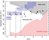 |
Fig. 10. Same as Fig. 9 but for the expected results from a simulation of 200 ks exposure with Athena X-IFU. |
The above result represents only a part of the absorption study possibilities for AGNs with future instruments. The spectral analysis using the tpho method has its limitations, as it needs a relatively long exposure to accumulate a high-quality time-integrated spectrum. On the other hand, timing analysis provides an alternative approach that is less constrained, since it does not require a comprehensive fitting of the full spectrum. The timing approach encompasses techniques that employ Fourier timing (Silva et al. 2016) and coherence analysis (Juráňová et al. 2022) to study short-timescale variability and employ the density-delay relation for longer timescales (Li et al. 2023). According to Juráňová et al. (2022), the coherence modeling alone could potentially yield a density accuracy of ≤70 − 80% with X-IFU for outflows in a typical narrow-line Seyfert 1 AGN. Furthermore, Li et al. (2023) suggest that the density-delay relation could be applied effectively when the source density falls within the range of approximately 1010–1013 m−3 in NGC 3783. By leveraging the strengths of all available tools, we will be able to maximize our capability to determine the density and distance of the warm absorbers in AGNs.
Acknowledgments
SRON is supported financially by NWO, the Netherlands Organization for Scientific Research.
References
- Arav, N., Chamberlain, C., Kriss, G. A., et al. 2015, A&A, 577, A37 [NASA ADS] [CrossRef] [EDP Sciences] [Google Scholar]
- Ballhausen, R., Kallman, T. R., Gu, L., & Paerels, F. 2023, ApJ, 956, 65 [NASA ADS] [CrossRef] [Google Scholar]
- Barret, D., Lam Trong, T., den Herder, J. W., et al. 2018, SPIE Conf. Ser., 10699, 106991G [Google Scholar]
- Behar, E. 2009, ApJ, 703, 1346 [NASA ADS] [CrossRef] [Google Scholar]
- Behar, E., Rasmussen, A. P., Blustin, A. J., et al. 2003, ApJ, 598, 232 [Google Scholar]
- Bentz, M. C., Williams, P. R., Street, R., et al. 2021, ApJ, 920, 112 [NASA ADS] [CrossRef] [Google Scholar]
- Blustin, A. J., Branduardi-Raymont, G., Behar, E., et al. 2002, A&A, 392, 453 [NASA ADS] [CrossRef] [EDP Sciences] [Google Scholar]
- Blustin, A. J., Page, M. J., Fuerst, S. V., Branduardi-Raymont, G., & Ashton, C. E. 2005, A&A, 431, 111 [CrossRef] [EDP Sciences] [Google Scholar]
- Chelouche, D., & Netzer, H. 2005, ApJ, 625, 95 [NASA ADS] [CrossRef] [Google Scholar]
- Di Gesu, L., Costantini, E., Arav, N., et al. 2013, A&A, 556, A94 [NASA ADS] [CrossRef] [EDP Sciences] [Google Scholar]
- Edmonds, D., Borguet, B., Arav, N., et al. 2011, ApJ, 739, 7 [NASA ADS] [CrossRef] [Google Scholar]
- Gabel, J. R., Crenshaw, D. M., Kraemer, S. B., et al. 2003, ApJ, 595, 120 [NASA ADS] [CrossRef] [Google Scholar]
- Gabel, J. R., Kraemer, S. B., Crenshaw, D. M., et al. 2005, ApJ, 631, 741 [NASA ADS] [CrossRef] [Google Scholar]
- Gonçalves, A. C., Collin, S., Dumont, A. M., et al. 2006, A&A, 451, L23 [NASA ADS] [CrossRef] [EDP Sciences] [Google Scholar]
- Goosmann, R. W., Holczer, T., Mouchet, M., et al. 2016, A&A, 589, A76 [NASA ADS] [CrossRef] [EDP Sciences] [Google Scholar]
- GRAVITY Collaboration (Amorim, A., et al.) 2021, A&A, 648, A117 [NASA ADS] [CrossRef] [EDP Sciences] [Google Scholar]
- Juráňová, A., Costantini, E., & Uttley, P. 2022, MNRAS, 510, 4225 [CrossRef] [Google Scholar]
- Kaastra, J. S., & Jansen, F. A. 1993, A&AS, 97, 873 [NASA ADS] [Google Scholar]
- Kaastra, J. S., Raassen, A. J. J., Mewe, R., et al. 2004, A&A, 428, 57 [NASA ADS] [CrossRef] [EDP Sciences] [Google Scholar]
- Kaastra, J. S., Detmers, R. G., Mehdipour, M., et al. 2012, A&A, 539, A117 [NASA ADS] [CrossRef] [EDP Sciences] [Google Scholar]
- Kaastra, J. S., Mehdipour, M., Behar, E., et al. 2018, A&A, 619, A112 [NASA ADS] [CrossRef] [EDP Sciences] [Google Scholar]
- Kallman, T., & Dorodnitsyn, A. 2019, ApJ, 884, 111 [NASA ADS] [CrossRef] [Google Scholar]
- Kaspi, S., Brandt, W. N., Netzer, H., et al. 2000, ApJ, 535, L17 [NASA ADS] [CrossRef] [Google Scholar]
- Kaspi, S., Brandt, W. N., Netzer, H., et al. 2001, ApJ, 554, 216 [NASA ADS] [CrossRef] [Google Scholar]
- Kaspi, S., Brandt, W. N., George, I. M., et al. 2002, ApJ, 574, 643 [NASA ADS] [CrossRef] [Google Scholar]
- Keshet, N., & Behar, E. 2022, ApJ, 934, 124 [NASA ADS] [CrossRef] [Google Scholar]
- Krolik, J. H., & Kriss, G. A. 1995, ApJ, 447, 512 [NASA ADS] [CrossRef] [Google Scholar]
- Krongold, Y., Nicastro, F., Brickhouse, N. S., et al. 2003, ApJ, 597, 832 [NASA ADS] [CrossRef] [Google Scholar]
- Krongold, Y., Nicastro, F., Brickhouse, N. S., Elvis, M., & Mathur, S. 2005, ApJ, 622, 842 [NASA ADS] [CrossRef] [Google Scholar]
- Laha, S., Reynolds, C. S., Reeves, J., et al. 2021, Nat. Astron., 5, 13 [NASA ADS] [CrossRef] [Google Scholar]
- Li, C., Kaastra, J. S., Gu, L., & Mehdipour, M. 2023, A&A, in press, https://doi.org/10.1051/0004-6361/202346520 [Google Scholar]
- Luminari, A., Nicastro, F., Krongold, Y., Piro, L., & Linesh Thakur, A. 2023, A&A, in press, https://doi.org/10.1051/0004-6361/202245600 [Google Scholar]
- Mao, J., Mehdipour, M., Kaastra, J. S., et al. 2019, A&A, 621, A99 [NASA ADS] [CrossRef] [EDP Sciences] [Google Scholar]
- Markowitz, A. 2005, ApJ, 635, 180 [NASA ADS] [CrossRef] [Google Scholar]
- Markowitz, A., Edelson, R., Vaughan, S., et al. 2003, ApJ, 593, 96 [NASA ADS] [CrossRef] [Google Scholar]
- Mehdipour, M., Kaastra, J. S., & Kallman, T. 2016, A&A, 596, A65 [NASA ADS] [CrossRef] [EDP Sciences] [Google Scholar]
- Mehdipour, M., Kaastra, J. S., Kriss, G. A., et al. 2017, A&A, 607, A28 [NASA ADS] [CrossRef] [EDP Sciences] [Google Scholar]
- Nandra, K., Barret, D., Barcons, X., et al. 2013, ArXiv e-prints [arXiv:1306.2307] [Google Scholar]
- Netzer, H., Kaspi, S., Behar, E., et al. 2003, ApJ, 599, 933 [NASA ADS] [CrossRef] [Google Scholar]
- Nicastro, F., Fiore, F., Perola, G. C., & Elvis, M. 1999, ApJ, 512, 184 [NASA ADS] [CrossRef] [Google Scholar]
- Peterson, B. M., Ferrarese, L., Gilbert, K. M., et al. 2004, ApJ, 613, 682 [Google Scholar]
- Reynolds, C. S. 1997, MNRAS, 286, 513 [NASA ADS] [CrossRef] [Google Scholar]
- Rogantini, D., Mehdipour, M., Kaastra, J., et al. 2022, ApJ, 940, 122 [NASA ADS] [CrossRef] [Google Scholar]
- Sadaula, D. R., Bautista, M. A., García, J. A., & Kallman, T. R. 2023, ApJ, 946, 93 [NASA ADS] [CrossRef] [Google Scholar]
- Scott, A. E., Brandt, W. N., Behar, E., et al. 2014, ApJ, 797, 105 [CrossRef] [Google Scholar]
- Silva, C. V., Uttley, P., & Costantini, E. 2016, A&A, 596, A79 [NASA ADS] [CrossRef] [EDP Sciences] [Google Scholar]
- Smith, R. K., Bautz, M., Bregman, J., et al. 2022, SPIE Conf. Ser., 12181, 1218121 [NASA ADS] [Google Scholar]
- Theureau, G., Bottinelli, L., Coudreau-Durand, N., et al. 1998, A&AS, 130, 333 [NASA ADS] [CrossRef] [EDP Sciences] [Google Scholar]
- Uttley, P., McHardy, I. M., & Papadakis, I. E. 2002, MNRAS, 332, 231 [Google Scholar]
- van Hoof, P. A. M., Van de Steene, G. C., Guzmán, F., et al. 2020, Contrib. Astron. Obs. Skalnate Pleso, 50, 32 [NASA ADS] [Google Scholar]
- Weigelt, G., Hofmann, K. H., Kishimoto, M., et al. 2012, A&A, 541, L9 [NASA ADS] [CrossRef] [EDP Sciences] [Google Scholar]
All Tables
All Figures
|
Fig. 1. Simulated light curve (upper panel) and the corresponding evolution of the average Fe charge of component 3 (lower panels). The average charge variations are shown as solid lines for gas densities of 1014, 1012, 1010, and 108 m−3, while the dashed curves illustrate the corresponding source light curves in the same period. As the gas density decreases, the response time to source variations becomes longer, resulting in flatter average charge variations. To highlight the response time differences across various densities, each panel presents a different total time period. |
| In the text | |
|
Fig. 2. Average concentration distributions of Fe ions obtained from simulation runs with gas densities of 108, 1011, and 1014 m−3 for component 3. The obtained ion concentrations are shown as red dots. The best-fit total concentration, depicted as black lines, is the sum of the two equilibrium components depicted as blue and green lines. The ionization parameters and the fractional contributions of the two equilibrium components are also shown. A single component is sufficient to fit the average concentration in the case of 108 m−3. |
| In the text | |
|
Fig. 3. Deviation of log ξ (a) and the dispersion of the Fe ion concentration (b) plotted as a function of gas densities for light curves with fractional variability ranging from 10% to 50% (the simulated light curve shown in Fig. 1 has an average fractional variability, Fvar, of ∼40%). The deviation of log ξ is calculated as the difference between the intrinsic value and the value obtained from a single equilibrium component fitting of the simulated Fe ion concentration distribution, such as the ones shown in Fig. 2. The curves representing the averages over the nine warm absorber components (see Table 1) are plotted for both the deviation and dispersion. |
| In the text | |
|
Fig. 4. Column densities of Fe in equilibrium and the time-evolving condition. The upper panel shows the total column density of Fe in equilibrium, with each individual component plotted in a different color. To capture the wide range of concentrations, which span several orders of magnitude, a logarithmic scale is employed. The lower panel compares the equilibrium column density (represented as a dashed black line) to the average column density of time-dependent photoionization, with gas densities of 108 and 1014 m−3 shown as blue and red lines. |
| In the text | |
|
Fig. 5. RXTE and Chandra HETGS light curves of NGC 3783 from mid-1999 to the end of 2001. The upper panel shows the RXTE proportional counter array data in the 2 − 60 keV band, with the average flux level indicated by a horizontal line. The Chandra HETGS light curves are presented in the panels below as red data points, along with the adjacent RXTE data converted using the PIMMS tool. |
| In the text | |
|
Fig. 6. Power spectral density function of the combined RXTE (black) and Chandra HETGS (red) light curves shown in Fig. 5. The data are compared with the model (dashed line) based on the best-fit results obtained in Markowitz (2005) on the data in the 0.2 − 12.0 keV range. |
| In the text | |
|
Fig. 7. Column densities of all Fe ions ranging from Fe IX to Fe XXVI determined through fitting using the slab model (black data points). The observed data points are compared with the values computed using the pion (red) and tpho (blue) models. Each panel represents one HETGS observation. |
| In the text | |
|
Fig. 8. Average charge states of Ne, Si, and Fe, as well as the combined column densities of Fe XIX and Fe XX, plotted as a function of the ionizing luminosity. The average charges are defined in Sect. 2. Each data point corresponds to an individual observation and was obtained via fitting with the slab model. The values obtained from the pion and tpho models are shown with red and blue curves, respectively. The χ-square values between the models and the data are displayed as numbers in the lower-right corner. |
| In the text | |
|
Fig. 9. Hydrogen number densities of the warm absorbers plotted as a function of their ionization parameters. Our results for components 1–5 from the tpho model are shown as stars. The gray shaded region represents the region where the outflow is unable to escape the gravitational potential of the black hole due to nH > nesc, while the dashed line indicates the position of |
| In the text | |
|
Fig. 10. Same as Fig. 9 but for the expected results from a simulation of 200 ks exposure with Athena X-IFU. |
| In the text | |
Current usage metrics show cumulative count of Article Views (full-text article views including HTML views, PDF and ePub downloads, according to the available data) and Abstracts Views on Vision4Press platform.
Data correspond to usage on the plateform after 2015. The current usage metrics is available 48-96 hours after online publication and is updated daily on week days.
Initial download of the metrics may take a while.