| Issue |
A&A
Volume 680, December 2023
|
|
|---|---|---|
| Article Number | A44 | |
| Number of page(s) | 12 | |
| Section | Extragalactic astronomy | |
| DOI | https://doi.org/10.1051/0004-6361/202346520 | |
| Published online | 07 December 2023 | |
Density calculations of NGC 3783 warm absorbers using a time-dependent photoionisation model
1
Leiden Observatory, Leiden University, PO Box 9513 2300 RA Leiden, The Netherlands
e-mail: This email address is being protected from spambots. You need JavaScript enabled to view it.
2
SRON Netherlands Institute for Space Research, Niels Bohrweg 4, 2333 CA Leiden, The Netherlands
3
Space Telescope Science Institute, 3700 San Martin Drive, Baltimore, MD 21218, USA
Received:
28
March
2023
Accepted:
21
August
2023
Abstract
Outflowing wind, as one type of AGN feedback involving non-collimated ionised winds such as those prevalent in Seyfert-1 AGNs, impacts the host galaxy by carrying kinetic energy outwards. However, the distance of the outflowing wind is poorly constrained because of a lack of direct imaging observations, which limits our understanding of its kinetic power, and thus of its impact on the local galactic environment. One potential approach to solving this problem involves determination of the density of the ionised plasma, making it possible to derive the distance using the ionisation parameter ξ, which can be measured based on the ionisation state. Here, by applying a new time-dependent photoionisation model, tpho, in SPEX, we define a new approach, the tpho-delay method, which we use to calculate or predict a detectable density range for warm absorbers of NGC 3783. The tpho model solves self-consistently the time-dependent ionic concentrations, which enables us to study the delayed states of the plasma in detail. We show that it is crucial to model the non-equilibrium effects accurately for the delayed phase, where the non-equilibrium and equilibrium models diverge significantly. Finally, we calculate the crossing time to consider the effect of the transverse motion of the outflow on the intrinsic luminosity variation. Future spectroscopic observations with more sensitive instruments are expected to provide more accurate constraints on the outflow density, and therefore on the feedback energetics.
Key words: X-rays: galaxies / galaxies: Seyfert / atomic processes / X-rays: individuals: NGC 3783
© The Authors 2023
 Open Access article, published by EDP Sciences, under the terms of the Creative Commons Attribution License (https://creativecommons.org/licenses/by/4.0), which permits unrestricted use, distribution, and reproduction in any medium, provided the original work is properly cited.
This article is published in open access under the Subscribe to Open model. This email address is being protected from spambots. You need JavaScript enabled to view it. to support open access publication.
1. Introduction
Outflows from active galactic nuclei (AGNs) have been found to carry significant kinetic energy, thereby impacting their host galaxy in a cosmic feedback mechanism, and leaving an imprint on the absorption spectrum in the UV and/or X-ray wavelength band (Laha et al. 2021).
With the assumption of spherical outflow (Blustin et al. 2005), the mass-outflow rate can be estimated via
 (1)
(1)
where the factor 1.23 takes into account the cosmic elemental abundances, mp is the mass of a proton, n(r) is the density of the outflow at radius r, Cv(r) is the volume-filling factor as a function of distance, and Ω is the solid angle subtended by the outflow. Subsequently, the kinetic luminosity  can be derived. From the spectral fitting of absorption lines and edges in UV/optical and X-rays, we can obtain the ionisation parameter (ξ) and the column density (NH) – which rely on Cv(r) and Ω –, and the outflow velocity (vout). However, the lack of spatial resolution in the inner parsec of the central engines makes it difficult to view these flows directly, further impeding measurement of the impact of AGN feedback.
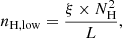
The ionisation parameter (Tarter et al. 1969; Krolik et al. 1981) conveniently quantifies the ionisation status of the outflows photoionised by the intense radiation from the accretion-driven central source, which is defined as
 (2)
(2)
where Lion is the 1 − 1000 Ryd (or 13.6 eV − 13.6 keV) band luminosity of the ionising source, nH the hydrogen number density of the ionised plasma, and r the distance of the plasma to the ionising source. Therefore, the distances can be constrained indirectly through measurements of the ionisation parameter, ionising luminosity, and density.
Assessing the density of the outflow accurately remains challenging. One approach is to use density-sensitive lines from a spectral analysis. The He-like triplet emission lines (Porquet et al. 2010) and the absorption lines from the metastable levels (Arav et al. 2015), among many other transitions, are considered to be sensitive to density. Mao et al. (2017) explored the density diagnostics using the metastable absorption lines of Be-, B-, and C-like ions for the AGN outflows, and found that in the same isoelectronic sequence, different ions cover not only a wide range of ionisation parameters but also an extensive density range. Less ionised ions probe lower density and smaller ionisation parameters within the same isonuclear sequence (Mao et al. 2017). The implementation of this method requires high-quality spectroscopic data of the outflows.
An alternative approach, namely spectral-timing analysis, mainly focuses on the variability of ionising luminosity, and involves investigation of the changes in the outflows over time, which can be a density-dependent response to the variation in the ionising luminosity (Kaastra et al. 2012; Rogantini et al. 2022). How fast the ionised plasma responds is dependent on the comparison of recombination timescale and the variability of the ionising source. Warm absorber (WA) as one kind of outflowing wind, can be studied using this technique. Through observations, it has been established that the response of WA to the continuum change provides valuable insight into the origin and acceleration mechanisms of this kind of outflow (Laha et al. 2021). Ebrero et al. (2016) estimated the lower limits on the density of WA of NGC 5548 with long-term variability using the photoionisation code Cloudy (Ferland et al. 1998). Time-dependent photoionisation modelling has been applied to Mrk 509 (Kaastra et al. 2012) and NGC 4051 (Silva et al. 2016), respectively, to constrain the density of WAs. It has been shown that the equilibrium model might become insufficient when it comes to detailed diagnostics of the outflows. The non-equilibrium model is needed to interpret high-quality data, including those obtained from future missions such as Athena (Sadaula et al. 2023; Juráňová et al. 2022).
Recently, Rogantini et al. (2022) built up a new time-dependent photoionisation model, tpho, which performs a self-consistent calculation solving the full time-dependent ionisation state for all ionic species and therefore allows investigation of time-dependent ionic concentrations. The tpho model keeps the shape of the spectral energy distribution (SED) constant, while the luminosity is able to be changed by following the input light-curve variation. In this paper, we apply this method with a realistic example of an AGN.
NGC 3783, with a redshift of z = 0.009730 (Theureau et al. 1998), hosts one of the most luminous local AGNs, with a bolometric AGN luminosity of log LAGN ∼ 44.5 erg s−1 at a distance of 38.5 Mpc (Davies et al. 2015) and also hosts a supermassive black hole of MBH = 3 × 10⁷ M⊙ (Vestergaard & Peterson 2006), and has been studied extensively, most notably for its ionised outflows (especially X-ray warm absorbers) and variability. In the X-ray band, ten photoionised components have been found (Mehdipour et al. 2017; Mao et al. 2019). The SED measured by Mehdipour et al. (2017) and the power spectral density (PSD) shape derived by Markowitz (2005), both in the unobscured state of NGC 3783, give us realistic parameters to feed into the tpho model.
In this study, we execute time-dependent photoionisation calculations using the tpho model (Rogantini et al. 2022) in SPEX version 3.07.01 (Kaastra et al. 2022) and adopt a realistic SED with variability and the ionisation parameters of ten WA components of NGC 3783 based on previous observations (Markowitz 2005; Mehdipour et al. 2017; Mao et al. 2019). In Sect. 2, we reproduce the measured SED and present the simulated light curve. In Sect. 3, we show tpho calculation results and execute a cross-correlation function to quantify the density-dependent lag; we also compare tpho with pion (photoionisation equilibrium model in SPEX). In Sects. 4 and 5, we discuss our findings and present conclusions.
2. Method
We first discuss how we produced a representative SED based on previous measurements, and simulated a realistic light curve corresponding to the PSD shape for NGC 3783. We assume that the shape of the SED stays the same during the variations. The tpho model calculates the evolution of ionic concentration for all available elements and all components of the WA. Finally, we show how we converted the ion concentration variation to the change of average charge states.
2.1. Modelling the NGC 3783 SED
We adopted the parameterised unobscured SED model of NGC 3783 determined by Mehdipour et al. (2017) for the unobscured state from 2000 to 2001 mainly based on the archival data taken by XMM-Newton (2000 and 2001) and Chandra HETGS (2000, 2001).
This model has a SED consisting of an optical/UV thin disc component, an X-ray power-law continuum, a neutral X-ray reflection component, and a warm Comptonisation component for the soft X-ray excess (Fig. 1).
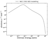 |
Fig. 1. Spectral energy distribution of NGC 3783 used in this work, based on Mehdipour et al. (2017) for the 2000 − 2001 observation in an unobscured state. |
2.2. Source simulated light curve
We used a doubly broken PSD (see Eq. (3)) model to simulate the NGC 3783 light curve (Markowitz 2005):
 (3)
(3)
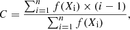
where Al is the PSD amplitude below the low-frequency break, fl = 2 × 10⁻⁷ Hz. Here the PSD has zero slopes. A = Al(fh/fl)−1 is the PSD amplitude at the high-frequency break, fh = 4 × 10⁻⁶ Hz. We adopt the best-fit Monte Carlo results from Table 2 of Markowitz (2005) and set the slope value to β = 2.6 as well as the power amplitude to A = 7200 Hz−1 in order to simulate the source light curve with variability in the energy band of 0.2 − 12 keV. The range between 2.5 × 10⁵ s and 5 × 10⁶ s becomes the typical timescale where high fluctuation occurs.
Figure 2 shows that the relative root-mean-square fluctuations decrease significantly as the binning time (hereafter tbin) increases from 105 to 107 s, while the variations on timescale ≤104 s remain nearly constant. Therefore, we (1) sample the light curve with bin size of 104 s and length of 1010 s or approximately 106 tbin, (2) and re-bin the light curve to 105 and/or 106 s bins for simulations with lower gas densities. For any densities of interest, the sampling time bin tbin is shorter than the typical recombination timescale of the WA.
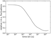 |
Fig. 2. Relative root-mean-square of fluctuations for different binning time of NGC 3783 based on Eq. (3). |
2.3. Ten WA components
We use the modelling based on the extensive observations with Chandra and XMM-Newton (Mehdipour et al. 2017). By analysing the archival Chandra and XMM-Newton grating data taken in 2000, 2001, and 2013, when the AGN was in an unobscured state, Mao et al. (2019) found nine photoionised absorption components with different ionisation parameters and kinematics. We incorporate them as components 1 − 9 in our current work. In the obscured state of the December 2016 data, Mehdipour et al. (2017) find evidence of a strong high-ionisation component (labelled HC in their Fig. 4), which is designated as component 0 in the present work. AGN SEDs do not normally change in shape significantly, unless there is strong X-ray obscuration, as in the above case. However, component 0, due to its high-ionisation state, is likely located near the centre and is therefore not shielded by the obscurer. It is therefore reasonable to assume that both component 0 and components 1 − 9 experience the same unobscured SED.
Table 1 shows the parameters of the ten WA components obtained with the pion model of SPEX. We use them as initial conditions for our tpho calculations.
pion good-fit parameters of ten X-ray WAs components of NGC 3783 (see Mehdipour et al. 2017 Table 1, and Table 3 of Mao et al. 2019).
2.4. Recombination timescale
Photoionisation or recombination of the ionised gas in response to changes in the ionising continuum will occur. For each specific ion Xi, the recombination timescale trec is the time that gas needs to respond to a decrease in the continuum; it depends on the local density and the ion population, following the equation (Bottorff et al. 2000; Ebrero et al. 2016):
![Mathematical equation: $$ \begin{aligned} t_{\rm rec}(X_{\rm i})=\left(\alpha _{\rm r}(X_{\rm i}) n_{\rm e} \left[\frac{f(X_{\rm i+1})}{f(X_{\rm i})} - \frac{\alpha _{\rm r}(X_{\rm i-1})}{\alpha _{\rm r}(X_{\rm i})} \right] \right)^{-1}, \end{aligned} $$](/articles/aa/full_html/2023/12/aa46520-23/aa46520-23-eq5.gif) (4)
(4)
where αr(Xi) is the recombination rate from ion Xi − 1 to ion Xi, and f(Xi) is the fraction of element X at the ionisation level i. The recombination rates αr are known from atomic physics, and the fractions f can be determined from the ionisation balance of the source. ne is the electron density.
For a cloud with known ionisation structure, trec ∝ 1/ne. Table 2 shows the column densities of the most relevant ions for each WA component, which were calculated using the model presented in Table 1 in an equilibrium state. Ebrero et al. (2016) use the ionic column densities of these most important ions to compute ne × trec, and they averaged the ne × trec of all the ions used to estimate it for the relevant WA component. The recombination timescale is defined this way through Eq. (4); however, it changes sign near the ion with the highest relative concentration and becomes very large in absolute value, meaning that this definition of the recombination timescale is not intuitive.
Ion column density NX in [1020 m−2] of the ten WA components for the specified Fe, S, Si, Mg, O, and N ions.
We therefore simply define the recombination timescale of an element as the time that the ionised plasma needs to change the average charge of the element by one charge state, namely:
 (5)
(5)
The average charge C is defined as
 (6)
(6)
and
![Mathematical equation: $$ \begin{aligned} \frac{\mathrm{d}C}{\mathrm{d}t} = \sum _{i=1}^{n} [f(X_{\rm i+1}) \alpha _r (X_{\rm i+1}) - f(X_{\rm i}) \alpha _r (X_{\rm i})] i , \end{aligned} $$](/articles/aa/full_html/2023/12/aa46520-23/aa46520-23-eq8.gif) (7)
(7)
where the denotation of f(Xi) and αr(Xi) are the same as shown in the Eq. (4). Table 3 shows examples of tC and trec where we see that the two values are consistent. Following the above calculation, we replace the previous definition of trec by tC in order to characterise the recombination timescale.
Ion species recombination timescale trec and element charge time tC using pion calculation for WA component 0 with log ξ = 3.61 as well as nH = 1010 m−3.
To quantity the relation between tC and ne, we use the logarithm of their product using the following equation
 (8)
(8)
where we express tC in seconds and ne in m−3. Table 4 shows the K(ξ, Z) value for the ten WA components from a pion calculation using Eq. (5) for Fe, S, Si, Mg, O, and N.
Quantity K(ξ, Z) for the ten WA components.
2.5. TPHO calculation
We now apply the tpho model to calculate the time evolution of each WA component of NGC 3783. The starting point of the tpho calculation is an equilibrium solution, which can be obtained from the pion model, ideally using the luminosity averaged over the entire simulation. Figure 3 shows the simulated light curve with a tbin of 104 s and 512 data points, resulting in a duration of 5.12 × 10⁶ s. The initial parameters, such as ionisation parameter ξ and column density NH, are taken from Table 1. We explore a range of hydrogen number density (nH) from 108 m−3 to 1015 m−3.
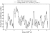 |
Fig. 3. NGC 3783 simulated light curve in the 0.2 − 12 keV band from the PSD shape of Markowitz (2005). |
If the photoionised plasma is too far away from the nucleus and/or the density of the plasma is too low, the plasma is in a quasi-steady state with its ionisation state varying slightly around the mean value, which corresponds to the mean ionising flux level over time; whereas for high density, the ion concentration will simultaneously follow the ionising luminosity variation in a near-equilibrium state (Krolik & Kriss 1995; Nicastro et al. 1999; Kaastra et al. 2012; Silva et al. 2016). Here we select the density range from 108 m−3 to 1015 m−3, which encompasses the steady state, the delayed state, and the nearby equilibrium state (see Sect. 3.1) as follows from our tpho calculation.
To further investigate the delayed state and to apply density diagnostics, the simulation must be set up with the following conditions,
 (9)
(9)
It is necessary to have tbin ≪ tvar because this guarantees that the variability of the ionising luminosity is sufficiently sampled. With tvar ≪ ttot, each simulation run would then contain multiple ionisation-recombination periods, providing better constraints. As addressed below, significant lags between the outflows and the central source are likely to be observed when tvar approaches the recombination time tC.
More specifically, we use tbin = 104, 105, 106 s for density 1012, 1011, 1010 m−3, respectively.
3. Results
We calculate the thermal stability curve of the ten WA components by computing the temperature for a range of ξ values using the pion model made with our SED. From this, we determine the pressure ionisation parameter, the ratio of radiation pressure to gas pressure, and Ξ defined as (Krolik et al. 1981)
 (10)
(10)
The shape of this curve in general depends on the precise form of the incoming X-ray spectrum. In this equation, p is the gas pressure, c is the speed of light, k is the constant of Boltzmann, and T is the electron temperature. Figure 4 shows a plot of log T versus log Ξ. We note that, in general, more temperature solutions are possible for a single value of Ξ (in particular when log Ξ is close to 1). Only solutions with dT/dΞ > 0 are stable, and therefore it seems that components 1 and 4 are in an unstable state.
 |
Fig. 4. Electron temperature in log T versus pressure ionisation parameter in log Ξ (‘S’ curve in black). The coloured dots show the ten X-ray WA components. |
Using the light curve described in Sect. 2.2 and the SED described in Sect. 2.1, we apply the tpho model for a range of densities for each WA component. The ion concentration changes over time because the gas ionises when the flux rises and recombines when the flux goes down. The recombination is responsible for the lag between the light curve and the ion concentration variability. We also investigate the relationship between density and lag timescales to further characterise this phenomenon. Here we present the component 0 results in more detail as an example.
3.1. Delayed state in ion concentration
Due to its high ionisation state, component 0 predominately produces absorption lines in the Fe-K band, and therefore we focus on Fe. We use the light curve with tbin = 104 s for the density ranging from 108 m−3 to 1015 m−3 in this section.
Figure 5 shows the ion concentrations of the most important Fe ions and the temperature as a function of time for three different densities. When the luminosity increases, the Fe XXVII concentration increases, but at the expense of Fe XXIV–Fe XXVI because of the conservation of the total number of Fe nuclei.
 |
Fig. 5. tpho calculation of the X-ray WA component 0 for NGC 3783 based on the simulated light curve (Fig. 3) and SED (Fig. 1). The time-dependent ion concentration of Fe XXVII, Fe XXVI, Fe XXV, and Fe XXIV are shown for hydrogen number densities of 1010, 1012, and 1014 m−3 in blue, red, and orange, respectively. The bottom panel shows the electron temperature T of the plasma of component 0 as a function of time. |
For a density of 1 × 10¹² m−3, the Fe XXVII ion concentration shows a clear lag with respect to the light curve. The lag arises mainly from the recombination timescale of the plasma, which depends inversely on the density (see Eq. (4)). Therefore, with increasing density, the Fe XXVII ion concentration (from blue, red, to orange curve) will correspond to a smaller lag timescale. For a higher density of 1 × 10¹⁴ m−3, the variability of Fe XXVII becomes well synchronised with the light curve. This is also the reason why the ion concentrations have a smoother appearance from high to low density. Further, the standard deviation amplitude of Fe XXVII for 1010, 1012, and 1014 m−3 is 0.007, 0.14, and 0.27, respectively.
The last panel of Fig. 5 shows the time-evolved electron temperature T profile. For low density, that is, 1010–1012 m−3, there are no variations and the temperature is constant over time, because the cooling rate is almost equal to the heating rate within the duration of the light curve. For higher density, for example 1014 m−3, the electron temperature lags because of the cooling time ∼106 s. Both time dependencies of the ion concentration and electron temperature are in agreement with the findings of (Rogantini et al. 2022; see their Figs. 7 and 8).
3.2. Density-dependent lag
The lag between the ionising luminosity and ion concentration as shown in Fig. 5 is caused by delayed recombination. To quantify the lag in our current work, we determine the cross-correlation function (CCF) between the average charge of Fe and the ionising luminosity as shown in Fig. 6. The Fe average charge CFe is derived using Eq. (6) for each time bin. The ionising luminosity L is also the value for each time bin. For both quantities, we calculate the relative variation by subtracting the long-term average. The CCF is a measure of the similarity of two series as a function of the displacement of one relative to the other as shown in the following equation:
![Mathematical equation: $$ \begin{aligned} ((L-\overline{L})*(C-\overline{C}))[\Delta t] = \sum _{-\infty }^{\infty } \overline{(L-\overline{L})[t]} (C-\overline{C})[t+\Delta t] . \end{aligned} $$](/articles/aa/full_html/2023/12/aa46520-23/aa46520-23-eq12.gif) (11)
(11)
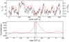 |
Fig. 6. Cross correlation of the Fe average charge with ionising luminosity for component 0 of NGC 3783. Top panel: Fe mean-subtracted average change (red curve) from the tpho calculation with a hydrogen number density of 1012 m−3 and an ionising luminosity in black (tbin = 104 s). Bottom: correlativity from CCF versus lag. The blue vertical line marks the lag timescale of 5 × 10⁴ s corresponding to the largest correlativity. |
Δt is defined as the displacement, also known as the lag. We use the procedure provided on the Scipy-correlation website1 to compute the CCF between the quantity  and mean-subtracted ionising luminosity (
 ). Here,
  and
and  are the average values calculated from all bins. We take the lag value corresponding to the largest correlativity for each calculation (see red curve at the bottom of Fig. 6).
Figure 6 shows the CCF for a hydrogen number density of 1012 m−3 and component 0. Here, we see a lag timescale of 5 × 10⁴ s (16 h, or more than half a day) for a density of 1012 m−3. There are lag timescales of 1 × 10⁶ and 2 × 10⁵ s for densities of 1010 and 1011 m−3, respectively. The uncertainties in the simulated light curve, which are derived from the power spectral density of Markowitz (2005), can introduce errors in the lag measurement. To account for this, we performed repeat simulations of the light curves, this time considering the errors in the observed PSD. By comparing the resulting lag times obtained from different light curves, we determine an uncertainty of roughly 10%.
The lag timescale in our work detected by the CCF method is the net effect of the recombination and ionisation periods. Similar to trec ∼ 1/n, the lag timescale decreases with increasing hydrogen number density because of the shorter recombination timescale, as shown in the top panel of Fig. 7. We fit these three data points (see black dot line) with a power law:
 (12)
(12)
 |
Fig. 7. Lag timescale and root-mean-square of average charge as a function of density for component 0 of NGC 3783 are presented in logarithmic. Top: lag timescale calculated from Fig. 6 vs. hydrogen number density in the unit of m−3. The fitting results are shown as a dashed line. Bottom: root-mean square σC of Fe average charge vs. hydrogen number density. The intersection between σC = −1.0 (horizontal black line) and the fitting results (dashed line) indicate the detectable lower limit. |
and find k = −0.651 and b = 12.489. Here, we find  for component 0. The observed lag, which is a result of both recombination and ionisation, is described by a power index of less than 1. Here, we take the timescale of 104 s as a typical minimum useful lag, which is approximately the timescale necessary to obtain a spectrum of sufficient quality so that AGN observations are relevant.
To scale the amplitude to the mean-subtracted average charge, we use root-mean-square 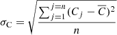 , where Cj refers to the average charge in the jth time binsize and n is the number of time bins. Hence, for each calculation from tpho, we further calculate the σC of the Fe ion concentration. At the bottom of Fig. 7, we show the relation between σC of Fe and hydrogen number density. We find that relatively high density corresponds to a relative large σC value, as well as a shorter lag time. We fit these three data points (see black dot line) with a power law:
 (13)
(13)
and find k = 0.357 and b = −5.111. We assume that, in practice, we can observe significant changes in absorption line spectra where σCFe > 0.1; however, for lower densities or longer lags, the amplitude of the charge variations becomes almost too small for effective measurement. Here, 10% serves as an empirical standard. A 10% variation in average charge for one element typically corresponds to changes of the order of 10% in ion concentration and therefore also in ionic column density and line optical depth. This is approximately true based on the observed Fe ion concentrations reported in Kaspi et al. (2002). For component 0, for Fe, we find a density of approximately 3 × 10¹¹ m−3 (see the black horizontal line) when σ = 0.1.
From the constraints of lag larger than 104 s and σC larger than 10%, for component 0 and Fe, lags can be detected for densities of roughly between 3 × 10¹¹ and 1 × 10¹³ m−3. Therefore, the above method – referred to here as the tpho-delay method – can be used to constrain the density range of the outflowing wind when the source variability timescale is comparable to the recombination time, that is, ionised plasma in delayed state. We carried out the same calculation for the other nine components.
3.3. Constraint on the WA density
Apart from the constraint that can be obtained from the spectral-timing analysis, that is, using the tpho-delay method of Sect. 3.2 in our present work, we take into account other astrophysical conditions. A lower limit to the density is obtained by assuming that the thickness (Δr) of the WA plasma cannot exceed its distance (r) to the SMBH (Krolik & Kriss 2001; Blustin et al. 2005), namely Δr ≤ r, and so we can derive the lower limit of the physical density using the following equation:
 (14)
(14)
where NH is the column density.
The upper limit to the density can be obtained based on the assumption that the outflow velocity vout of the wind is larger than or equal to the escape velocity (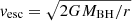 ); see for example Blustin et al. (2005). This gives,
 (15)
(15)
Using MBH = 3 × 10⁷ M⊙ (Vestergaard & Peterson 2006) and other parameters from Table 1, we compute nH, low and nH, upp.
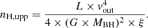
Following the technique introduced in Mao et al. (2017), we calculated the ranges of detectable densities using absorption lines from metastable levels in C-like ions for NGC 3783. The parameter range covered by this method shows a dependence on ionisation parameter and density, as depicted in the coloured rectangles of Fig. 8, which shows a comprehensive constraint on the density ranges for all ten WA components as derived from the methods described above.
 |
Fig. 8. Detectable density ranges of 10 X-ray WA components in the unobscured state of NGC 3783. The 10 WAs are marked in red. Upper black points and line: outflow velocity equals the escape velocity. For higher densities, winds cannot escape i.e., they are failed winds as shown in the light azure shaded region. Lower black points and line: the thickness of the wind equals its distance to the core. For lower densities, no solution exists, i.e., forbidden region shown in the yellow region. Red vertical solid lines: the detectable density range by the tpho-delay method for all 10 X-ray WAs. The upper limit: lag equals 104 s. For higher densities, lags are shorter and more difficult to measure due to photon statistics. The lower limit: relative variations of the charge of Fe ions is 10%. For lower densities, variations become too small to measure. Navy stars and lines with labels 1a–3: density measurements or lower limits from Gabel et al. (2005). ξ values converted for models with the SED of Mehdipour et al. (2017). Rectangular boxes: regions where density-sensitive X-ray lines can be used to measure densities. |
V = Vesc and Δr = r derived from previous observation are taken as the upper and lower limits on the density for the margins of a failed wind and the forbidden region, respectively. For X-ray component 0, we find that 1012.2 < nH < 1011.8 m−3, which means the lower limit is higher than the upper limit, and therefore that X-ray component 0 is a possible candidate for a failed wind.
We see that for the components with a relatively narrow physical density range as well as higher ionisation parameters, such as components 1 − 4, the tpho-delay method provides powerful diagnostics for the failed-wind scenario. The detectable density range of the tpho-delay method for components 2 − 5 covers most of their available physical density range, and therefore their density can be determined well using our method. Starting from component 5, metastable density works, and Si IX and S XI can be used to diagnose whether component 5 is failed wind or not.
For components 6 − 9 with a relatively broad allowed physical density range and a low ionisation parameter, we can combine the tpho-delay method with metastable C-like ions to give density constraints in the X-ray band. For components 7 − 9, we can cross-check between tpho-delay and the Ne V metastable lines. Mg VII, Ne V, and O III metastable lines also expand the detectable density range for components 6 − 9.
Grey stars and lines represent the density measurements or lower limit from UV observations using the UV metastable absorption lines (Table 3 in Gabel et al. 2005). Their ionisation parameter UH = QH/4πcnHr2 was converted into ξ for the models with the SED and luminosity of Mehdipour et al. (2017). We discuss UV components further in Sect. 5.
We note that here we use tlagFe, which is the lag timescale of the Fe average charge, to give the detectable density range for components at different ionisation states. However, the other elements would complement Fe in particular for the low-ionisation components. To fully comprehend the behaviour of the WA outflows, we will need to conduct similar calculations for other critical elements, such as C, O, N, Mg, and Si.
3.4. TPHO versus PION
In the present work, we derive the density of ionised plasma using the tpho model. In tpho calculations, the ξ value simply scales with the time-dependent luminosity value, assuming that the product nH × r2 remains constant over time. Thus,
 (16)
(16)
where L° and ξ° are the luminosity and ionisation parameter at t = 0, which is assumed to be in equilibrium state.
The pion model assumes photoionisation equilibrium, and the ionisation parameter ξ is obtained by fitting the observed spectra. Once the ξ value is known, the ion concentrations of different elements are known and the corresponding elemental average charge is also determined. There is therefore a one-to-one relation between ξPION and the element average charge in the pion equilibrium state.
In the left panels of Fig. 9, the black dots represent the ξ values of the pion model that are needed to yield the same Fe average charge value as the CFe(t) from the tpho simulation, which is represented by ξTPHO(t). The red line corresponds to equal values of both quantities. Only a small fraction of data points are located on the red line, which corresponds to the equilibrium state.
 |
Fig. 9. Ionisation parameter and Fe ion average charge comparisons for tpho and pion for X-ray WA component 0 of NGC 3783 for three different densities (1010, 1011 and 1012 m−3 from top to bottom). In the left panels, the black dots represent the ξ values of pion that are needed to obtain the same Fe average charge as for the tpho model. ξTPHO is a luminosity-dependent quantity in tpho calculations (See Eq. (16)). The red line represents the condition where the log ξ from pion is equal to tpho. The right panels show log ξ versus CFe, where the blue dots represent the pion log ξ and red dots represent the tpho log ξ, respectively. |
This figure also shows the limitations of applying an equilibrium (pion) model to a source that in reality has time-dependent photoionisation, as represented by the realistic tpho model. This holds in particular for periods of low luminosity (low ξTPHO(t)). In the right panels of Fig. 9, for example, nH = 1012 m−3, the data point with the lowest ξTPHO value of 2.75 (in the log) has an average charge for Fe of 25.4; if the corresponding spectrum were fitted with an equilibrium pion model, this average charge would yield log ξ = 3.5, a ξ value that is 5.6 times larger than the tpho value. Because the observer would like to use the measured luminosity for this data point to derive the product nH × r2 = Lion/ξ, both the lower L and larger ξ would lead to underestimation of nH × r2 by more than an order of magnitude.
4. Discussion
4.1. Ten WAs of NGC 3783 detectable geometry distance
We used Eq. (2) to derive the detectable distance based on our lag density relation in the present work and compared it with the NGC 3783 intrinsic structure measured by GRAVITY Collaboration (2021) as shown in Fig. 10. Component 0 exhibits a detectable distance very close to the broad line region, while components 1 − 2 can be constrained within the host dust structure. Components 1 − 4 show a relatively large detectable distance range, typically within approximately 1 parsec, which corresponds to the torus structure. Additionally, the distances of components 5 − 9 are detectable with our method only when they are located outside the torus.
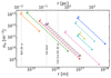 |
Fig. 10. Ten WAs for NGC 3783 used to predict the detectable distance range with the tpho-delay method (shown as a coloured dashed line). The vertical dashed lines show the main components of the structure measured by GRAVITY Collaboration (2021). |
4.2. Correspondence with the UV-X-ray absorbers
In addition to the ten X-ray WAs, there are absorbers detected in UV (Kraemer et al. 2001; Gabel et al. 2005) that exhibit some features in common with the chosen X-ray counterpart. Figure 8 shows three UV absorbers reported in Gabel et al. (2005), in which component 1 is composed of two physically distinct regions (1a and 1b) detected by the difference in covering factor and kinematic structure. Both components 1a and 1b are assumed to be colocated, because there is a decrease in the radial velocity of the lines in both components together with the same outflowing velocity (bottom panel of Fig. 11), while the ionisation parameter for component 1b derived in the unsaturated red wing of C IV and N V is higher than that of 1a, and therefore component 1b has lower density and column density (top panel of Fig. 11). The electron density of the lower ionisation component 1a, ∼3 × 10¹⁰ m−3, which we obtained directly from the individual metastable levels, falls in the range where the tpho-delay method as well as the metastable lines of Ne V can provide useful constraints. Moreover, UV component 1a appears to be intimately linked to component 9 in the X-rays. Therefore, UV component 1a can serve as a calibration for density diagnostic using an X-ray detector.
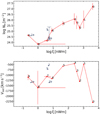 |
Fig. 11. Ten X-ray WA components and four UV components (Gabel et al. 2005) in NGC 3783 observations. Top panel: NH versus log ξ. Bottom panel: Vout versus log ξ. |
Direct estimates of density are not available for UV components 2 and 3 and so these are less well constrained than component 1 (Fig. 8). The lower limits on their densities are derived based on the basis of the observed variability. The ionisation parameters from higher ionisation UV absorbers, components 1b, 2, and 3 with log ξ ∼ 0.7, are close to the X-ray component 7 with log ξ ∼ 0.6. Nevertheless, the latter has a smaller total column density (Fig. 11).
Although the above findings suggest a possible connection between the UV absorbers and the weakly ionised X-ray counterparts, this connection remains uncertain given the poor X-ray constraints. It will be possible to test this hypothesis using the high-resolution X-ray data obtained with the upcoming XRISM (XRISM Science Team 2022) and Athena missions (Nandra et al. 2013).
4.3. Crossing time
X-ray variability from black holes is generally characterised as a red noise process (Uttley et al. 2014), and can be caused by different physical radiation processes (Cackett et al. 2021). Gabel et al. (2003) note that the observed changes in the absorption components could be due to the transverse motion of the clumping wind that moves across the line of sight, but for the intrinsic luminosity variability. To determine the potential impact of Keplerian motions on WA variability, we calculated the crossing time of outflows and compared them with the recombination time.
The X-ray-emitting region has a scale no larger than 20 gravitational radii (Reis & Miller 2013) as shown in the following equation,
 (17)
(17)
Therefore, the crossing time tcross can be computed as
 (18)
(18)
where  . Substituting Eq. (2) and Eq. (17) into Eq. (18), we obtain
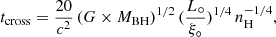 (19)
(19)
where L° = 6.36 × 1036 W (Mehdipour et al. 2017), and ξ° comes from Table 1.
The three timescales in Fig. 12, charge time tCFe, lag timescale tlagFe, and crossing time tcross, are density-dependent. We also present the positions of density constraints from tpho-delay and other methods.
 |
Fig. 12. Comparing tCFe, tlagFe, and tcross of the ten X-ray WAs in NGC 3783. The dashed and dotted line notations are the same as in Fig. 8. |
These findings show that the density ranges where our tpho-delay method can offer useful constraints likely satisfy tCFe < tcross. This indicates that the transverse motion of the outflows may not have a significant impact on the density diagnostics obtained assuming luminosity variation, that is, the ionisation variation is likely to be mainly caused by the variability, and not the transverse motions. We therefore consider the tpho-delay methods to be largely valid, even when accounting for the potential variability driven by motion.
4.4. SED and light curve of NGC 3783
The AGN SEDs do not normally change their shape significantly unless something dramatic happens; as in changing-look AGN, where the accretion rate and the X-ray corona emission decline. The SED may also vary if there is strong X-ray obscuration, and the difference between the impact of obscured and unobscured SEDs on the ionisation state is significant, as shown in NGC 5548 (Mehdipour et al. 2016). Here, the SED we used is uniformly derived from an unobscured state in order to study the ionisation state of the ten WA components. Because component 0 is in the obscured state but is not shielded by the obscurer, it is reasonable to assume that the same SED can be used for component 0 and components 1 − 9. NGC 3783 is a Seyfert-1 galaxy, and no extreme changing-look accretion events have been observed for this object. It is therefore reasonable to conclude that it is the normalisation that is mostly changing in an unobscured state. Indeed, individual SED components (such as the soft excess) show some specific variability, but usually this does not cause the shape to change so much such that it would impact photoionisation. Therefore, for tpho to assume that only the normalisation of the SED is changing is sufficient approximation in this case. We also note that deriving the variability of the SED shape (with limited data) presents certain challenges and entails assumptions that are highly model dependent.
4.5. Comparison with other time-resolved analyses
Time-dependent photoionisation modelling for outflowing winds has been described in other papers, but with different model constructions. Silva et al. (2016) and Juráňová et al. (2022) carry out time-dependent photoionisation modeling using precalculated runs from Cloudy, assuming equilibrium conditions. However, the tpho model Rogantini et al. (2022) takes into account non-equlibrium state conditions and tracks the time-dependency of the heating and cooling process according to the light curve of the ionising SED.
We point out that, without considering the non-equilibrium time-dependency of the heating and cooling process, it will, to some extent, affect the resulting calculation of ion concentration, because recombination rates are not only a function of density but also of temperature. A long light-curve history is required for tpho input, and the upcoming new satellite XRISM can provide good spectra to compare with the models. tpho is expected to be able to fit the observational data in cases where no significant change is seen in the shapes of AGN SEDs.
5. Conclusions
By using a realistic SED with variability from a realistic PSD, and WA physical parameters based on previous X-ray observations, we performed a theoretical tpho model calculation to investigate the time-dependent photoionisation plasma state of ten WA components of NGC 3783. We employed cross-correlation calculations to measure the correlation between response lag time and the outflow density for all WA components. By doing so, we determined the ranges of density for which the tpho model can yield practical constraints, and we compared our results with those obtained from metastable absorption lines in X-ray and UV bands. We further demonstrate that Keplerian motion is likely to have negligible impact on the density measurement for our range of interest. Our technique can easily be applied to the new data obtained with upcoming X-ray missions including XRISM and Athena.
Acknowledgments
We thank the anonymous referee for his/her constructive comments. C.L. acknowledges support from Chinese Scholarship Council (CSC) and Leiden University/Leiden Observatory, as well as SRON. SRON is supported financially by NWO, the Netherlands Organization for Scientific Research. C.L. thanks Anna Juráová for the discussions of different time-dependent photoionisation model constructions.
References
- Arav, N., Chamberlain, C., Kriss, G. A., et al. 2015, A&A, 577, A37 [NASA ADS] [CrossRef] [EDP Sciences] [Google Scholar]
- Blustin, A. J., Page, M. J., Fuerst, S. V., Branduardi-Raymont, G., & Ashton, C. E. 2005, A&A, 431, 111 [CrossRef] [EDP Sciences] [Google Scholar]
- Bottorff, M. C., Korista, K. T., & Shlosman, I. 2000, ApJ, 537, 134 [NASA ADS] [CrossRef] [Google Scholar]
- Cackett, E. M., Bentz, M. C., & Kara, E. 2021, iScience, 24, 102557 [NASA ADS] [CrossRef] [Google Scholar]
- Davies, R. I., Burtscher, L., Rosario, D., et al. 2015, ApJ, 806, 127 [Google Scholar]
- Ebrero, J., Kaastra, J. S., Kriss, G. A., et al. 2016, A&A, 587, A129 [NASA ADS] [CrossRef] [EDP Sciences] [Google Scholar]
- Ferland, G. J., Korista, K. T., Verner, D. A., et al. 1998, PASP, 110, 761 [Google Scholar]
- Gabel, J. R., Crenshaw, D. M., Kraemer, S. B., et al. 2003, ApJ, 595, 120 [NASA ADS] [CrossRef] [Google Scholar]
- Gabel, J. R., Kraemer, S. B., Crenshaw, D. M., et al. 2005, ApJ, 631, 741 [NASA ADS] [CrossRef] [Google Scholar]
- GRAVITY Collaboration (Amorim, A., et al.) 2021, A&A, 648, A117 [NASA ADS] [CrossRef] [EDP Sciences] [Google Scholar]
- Juráňová, A., Costantini, E., & Uttley, P. 2022, MNRAS, 510, 4225 [CrossRef] [Google Scholar]
- Kaastra, J. S., Detmers, R. G., Mehdipour, M., et al. 2012, A&A, 539, A117 [NASA ADS] [CrossRef] [EDP Sciences] [Google Scholar]
- Kaastra, J. S., Raassen, A. J. J., de Plaa, J., & Gu, L. 2022, https://doi.org/10.5281/zenodo.7037609 [Google Scholar]
- Kaspi, S., Brandt, W. N., George, I. M., et al. 2002, ApJ, 574, 643 [NASA ADS] [CrossRef] [Google Scholar]
- Kraemer, S. B., Crenshaw, D. M., & Gabel, J. R. 2001, ApJ, 557, 30 [NASA ADS] [CrossRef] [Google Scholar]
- Krolik, J. H., & Kriss, G. A. 1995, ApJ, 447, 512 [NASA ADS] [CrossRef] [Google Scholar]
- Krolik, J. H., & Kriss, G. A. 2001, ApJ, 561, 684 [CrossRef] [Google Scholar]
- Krolik, J. H., McKee, C. F., & Tarter, C. B. 1981, ApJ, 249, 422 [NASA ADS] [CrossRef] [Google Scholar]
- Laha, S., Reynolds, C. S., Reeves, J., et al. 2021, Nat. Astron., 5, 13 [NASA ADS] [CrossRef] [Google Scholar]
- Mao, J., Kaastra, J. S., Mehdipour, M., et al. 2017, A&A, 607, A100 [NASA ADS] [CrossRef] [EDP Sciences] [Google Scholar]
- Mao, J., Mehdipour, M., Kaastra, J. S., et al. 2019, A&A, 621, A99 [NASA ADS] [CrossRef] [EDP Sciences] [Google Scholar]
- Markowitz, A. 2005, ApJ, 635, 180 [NASA ADS] [CrossRef] [Google Scholar]
- Mehdipour, M., Kaastra, J. S., & Kallman, T. 2016, A&A, 596, A65 [NASA ADS] [CrossRef] [EDP Sciences] [Google Scholar]
- Mehdipour, M., Kaastra, J. S., Kriss, G. A., et al. 2017, A&A, 607, A28 [NASA ADS] [CrossRef] [EDP Sciences] [Google Scholar]
- Nandra, K., Barret, D., Barcons, X., et al. 2013, ArXiv e-prints [arXiv:1306.2307] [Google Scholar]
- Nicastro, F., Fiore, F., Perola, G. C., & Elvis, M. 1999, ApJ, 512, 184 [NASA ADS] [CrossRef] [Google Scholar]
- Porquet, D., Dubau, J., & Grosso, N. 2010, Space. Sci. Rev., 157, 103 [NASA ADS] [CrossRef] [Google Scholar]
- Reis, R. C., & Miller, J. M. 2013, ApJ, 769, L7 [NASA ADS] [CrossRef] [Google Scholar]
- Rogantini, D., Mehdipour, M., Kaastra, J., et al. 2022, ApJ, 940, 122 [NASA ADS] [CrossRef] [Google Scholar]
- Sadaula, D. R., Bautista, M. A., Garcia, J. A., & Kallman, T. R. 2023, ApJ, 946, 93 [NASA ADS] [CrossRef] [Google Scholar]
- Silva, C. V., Uttley, P., & Costantini, E. 2016, A&A, 596, A79 [NASA ADS] [CrossRef] [EDP Sciences] [Google Scholar]
- Tarter, C. B., Tucker, W. H., & Salpeter, E. E. 1969, ApJ, 156, 943 [Google Scholar]
- Theureau, G., Bottinelli, L., Coudreau-Durand, N., et al. 1998, A&AS, 130, 333 [NASA ADS] [CrossRef] [EDP Sciences] [Google Scholar]
- Uttley, P., Cackett, E. M., Fabian, A. C., Kara, E., & Wilkins, D. R. 2014, A&ARv, 22, 72 [NASA ADS] [CrossRef] [Google Scholar]
- Vestergaard, M., & Peterson, B. M. 2006, ApJ, 641, 689 [Google Scholar]
- XRISM Science Team 2022, ArXiv e-prints [arXiv:2202.05399] [Google Scholar]
All Tables
pion good-fit parameters of ten X-ray WAs components of NGC 3783 (see Mehdipour et al. 2017 Table 1, and Table 3 of Mao et al. 2019).
Ion column density NX in [1020 m−2] of the ten WA components for the specified Fe, S, Si, Mg, O, and N ions.
Ion species recombination timescale trec and element charge time tC using pion calculation for WA component 0 with log ξ = 3.61 as well as nH = 1010 m−3.
All Figures
|
Fig. 1. Spectral energy distribution of NGC 3783 used in this work, based on Mehdipour et al. (2017) for the 2000 − 2001 observation in an unobscured state. |
| In the text | |
|
Fig. 2. Relative root-mean-square of fluctuations for different binning time of NGC 3783 based on Eq. (3). |
| In the text | |
|
Fig. 3. NGC 3783 simulated light curve in the 0.2 − 12 keV band from the PSD shape of Markowitz (2005). |
| In the text | |
|
Fig. 4. Electron temperature in log T versus pressure ionisation parameter in log Ξ (‘S’ curve in black). The coloured dots show the ten X-ray WA components. |
| In the text | |
|
Fig. 5. tpho calculation of the X-ray WA component 0 for NGC 3783 based on the simulated light curve (Fig. 3) and SED (Fig. 1). The time-dependent ion concentration of Fe XXVII, Fe XXVI, Fe XXV, and Fe XXIV are shown for hydrogen number densities of 1010, 1012, and 1014 m−3 in blue, red, and orange, respectively. The bottom panel shows the electron temperature T of the plasma of component 0 as a function of time. |
| In the text | |
|
Fig. 6. Cross correlation of the Fe average charge with ionising luminosity for component 0 of NGC 3783. Top panel: Fe mean-subtracted average change (red curve) from the tpho calculation with a hydrogen number density of 1012 m−3 and an ionising luminosity in black (tbin = 104 s). Bottom: correlativity from CCF versus lag. The blue vertical line marks the lag timescale of 5 × 10⁴ s corresponding to the largest correlativity. |
| In the text | |
|
Fig. 7. Lag timescale and root-mean-square of average charge as a function of density for component 0 of NGC 3783 are presented in logarithmic. Top: lag timescale calculated from Fig. 6 vs. hydrogen number density in the unit of m−3. The fitting results are shown as a dashed line. Bottom: root-mean square σC of Fe average charge vs. hydrogen number density. The intersection between σC = −1.0 (horizontal black line) and the fitting results (dashed line) indicate the detectable lower limit. |
| In the text | |
|
Fig. 8. Detectable density ranges of 10 X-ray WA components in the unobscured state of NGC 3783. The 10 WAs are marked in red. Upper black points and line: outflow velocity equals the escape velocity. For higher densities, winds cannot escape i.e., they are failed winds as shown in the light azure shaded region. Lower black points and line: the thickness of the wind equals its distance to the core. For lower densities, no solution exists, i.e., forbidden region shown in the yellow region. Red vertical solid lines: the detectable density range by the tpho-delay method for all 10 X-ray WAs. The upper limit: lag equals 104 s. For higher densities, lags are shorter and more difficult to measure due to photon statistics. The lower limit: relative variations of the charge of Fe ions is 10%. For lower densities, variations become too small to measure. Navy stars and lines with labels 1a–3: density measurements or lower limits from Gabel et al. (2005). ξ values converted for models with the SED of Mehdipour et al. (2017). Rectangular boxes: regions where density-sensitive X-ray lines can be used to measure densities. |
| In the text | |
|
Fig. 9. Ionisation parameter and Fe ion average charge comparisons for tpho and pion for X-ray WA component 0 of NGC 3783 for three different densities (1010, 1011 and 1012 m−3 from top to bottom). In the left panels, the black dots represent the ξ values of pion that are needed to obtain the same Fe average charge as for the tpho model. ξTPHO is a luminosity-dependent quantity in tpho calculations (See Eq. (16)). The red line represents the condition where the log ξ from pion is equal to tpho. The right panels show log ξ versus CFe, where the blue dots represent the pion log ξ and red dots represent the tpho log ξ, respectively. |
| In the text | |
|
Fig. 10. Ten WAs for NGC 3783 used to predict the detectable distance range with the tpho-delay method (shown as a coloured dashed line). The vertical dashed lines show the main components of the structure measured by GRAVITY Collaboration (2021). |
| In the text | |
|
Fig. 11. Ten X-ray WA components and four UV components (Gabel et al. 2005) in NGC 3783 observations. Top panel: NH versus log ξ. Bottom panel: Vout versus log ξ. |
| In the text | |
|
Fig. 12. Comparing tCFe, tlagFe, and tcross of the ten X-ray WAs in NGC 3783. The dashed and dotted line notations are the same as in Fig. 8. |
| In the text | |
Current usage metrics show cumulative count of Article Views (full-text article views including HTML views, PDF and ePub downloads, according to the available data) and Abstracts Views on Vision4Press platform.
Data correspond to usage on the plateform after 2015. The current usage metrics is available 48-96 hours after online publication and is updated daily on week days.
Initial download of the metrics may take a while.