| Issue |
A&A
Volume 694, February 2025
|
|
|---|---|---|
| Article Number | A302 | |
| Number of page(s) | 9 | |
| Section | Extragalactic astronomy | |
| DOI | https://doi.org/10.1051/0004-6361/202452911 | |
| Published online | 20 February 2025 | |
A failed wind candidate in NGC 3783 from the 2001 campaign with Chandra/HETGS
1
Leiden Observatory, Leiden University, PO Box 9513 2300 RA Leiden, The Netherlands
2
SRON Netherlands Institute for Space Research, Niels Bohrweg 4, 2333 CA Leiden, The Netherlands
3
Department of Astronomy and Astrophysics, The University of Chicago, Chicago, IL 60637, USA
4
MIT Kavli Institute for Astrophysics and Space Research, Massachusetts Institute of Technology, Cambridge, MA 02139, USA
5
Space Telescope Science Institute, 3700 San Martin Drive, Baltimore, MD 21218, USA
⋆ Corresponding author; cli@strw.leidenuniv.nl
Received:
6
November
2024
Accepted:
15
January
2025
We reanalyse the Chandra/HETGS observations of NGC 3783 from the campaign in the year 2001 and identify significant spectral variations in the Fe unresolved transition array (UTA) over timescales of weeks to months. These changes correlate with a 1.4− to two-fold increase in the ionising continuum and exceed 10σ significance. The variations primarily originate from a low-ionisation state (log ξ = 1.65) component of the warm absorber. Time-dependent photoionisation modelling confirmed the sensitivity of this low-ionisation component to continuum variations within the Fe UTA band. Local fitting indicated a lower density limit of > 1012.3 m−3 at a 3σ statistical uncertainty, with the component located within 0.27 pc. Our findings suggest that this low-ionisation component is a potential failed wind candidate.
Key words: methods: observational / methods: statistical / galaxies: active / galaxies: individual: NGC 3783 / galaxies: nuclei / galaxies: Seyfert
© The Authors 2025
 Open Access article, published by EDP Sciences, under the terms of the Creative Commons Attribution License (https://creativecommons.org/licenses/by/4.0), which permits unrestricted use, distribution, and reproduction in any medium, provided the original work is properly cited.
This article is published in open access under the Subscribe to Open model. Subscribe to A&A to support open access publication.
1. Introduction
NGC 3783, a nearby Seyfert 1 galaxy at redshift z = 0.009730 (Theureau et al. 1998), hosts one of the most luminous local AGNs, with bolometric luminosity of log LAGN ∼ 44.5 erg s−1 at a distance of 38.5 Mpc (Davies et al. 2015). The AGN is powered by a supermassive black hole with  (Bentz et al. 2021). Extensive studies have focused on its ionised outflow, particularly the X-ray warm absorbers near the nucleus. While near-infrared interferometry has partially resolved the spatial structure of the broad-line region (BLR) within the central parsec (GRAVITY Collaboration 2021), a lack of direct imaging limits precise distance measurements of ionised plasma, including the warm absorber. This limits the ability to accurately determine the kinetic power and mass outflow rate of these absorbers.
The ionisation parameter

serves as a proxy for the outflow distance from the ionising source, where Lion is the ionising luminosity over the 1−1000 Ryd range, nH is the hydrogen number density, and r is the distance from the ionizing source (Tarter et al. 1969; Krolik et al. 1981). By measuring ξ, Lion, and nH, we can indirectly estimate the distance of the outflow.
Two main approaches can be used to derive the density for AGN outflows. The first relies on density-sensitive metastable spectral lines, which require high-quality, high-resolution spectra (often from time-averaged observations). For example, using the spectral energy distribution (SED) of NGC 5548, Mao et al. (2017) studied density diagnostics for AGN outflows through metastable absorption lines of Be-, B-, and C-like ions, showing that different ions within the same isoelectronic sequence can cover a broad range of ionisation parameters and densities. This technique has been used successfully to constrain the density of the lower ionised gas in NGC 3783 using UV lines (Gabel et al. 2005).
Another approach, the spectral-timing method uses time-resolved spectra to analyse plasma responses to fluctuations in ionising luminosity (Kaastra et al. 2012; Silva et al. 2016; Juráňnová et al. 2022). Time-dependent photoionisation modelling provides a comprehensive framework, simultaneously solving for ion concentration, heating, and cooling evolution in response to SED and AGN variability (Rogantini et al. 2022; Sadaula et al. 2023). The evolution of plasma state, indicated by the average charge over time, is driven by the relationship between the variability timescale (tvar) and the recombination timescale (trec), where trec is inversely proportional to plasma density. When tvar and trec are comparable, measurable lag timescales emerge between ionising luminosity changes and plasma state variations, given adequate sampling and photon counts in individual spectra (Li et al. 2023).
Variability in spectral lines correlated with flux changes has been observed in high signal-to-noise, high-resolution absorption spectroscopic studies (Netzer et al. 2003; Krongold et al. 2005). Analysing the 900 ks Chandra/HETG spectrum of NGC 3783, (Kaspi et al. 2002) provided a comprehensive characterisation of the absorption spectrum, which included several significant iron features, such as the L-shell lines from Fe XVII to Fe XXIV as well as the Unresolved Transition Array (UTA) of M-shell lines. The distinct Fe UTA structure has also been detected in XMM-Newton Reflection Grating Spectrometer spectra (Behar et al. 2001; Blustin et al. 2002). Various photoionisation models have been applied to analyse the X-ray absorption spectra of NGC 3783, and they employ different configurations: two ionised components (Blustin et al. 2002; Krongold et al. 2003, 2005), three components (Netzer et al. 2003), five components (Ballhausen et al. 2023), and nine components (Mehdipour et al. 2017; Kaastra et al. 2018; Mao et al. 2019). These models typically assume photoionisation equilibrium. However, Gu et al. (2023) introduced time-dependent effects within a nine-component photoionisation model, constraining the warm absorber’s density to the range 1010 − 1013 m−3.
Using the new time-dependent photoionisation model, tpho (Rogantini et al. 2022) in the SPEX code (Kaastra et al. 2024), we performed a self-consistent calculation of the full time-dependent ionisation state for all ionic species, generating synthetic transmission spectra based on the observed light curve. The structure of the paper is as follows. Section 2 presents the data reduction process for the Chandra/HETGS observations, incorporating recent calibration updates and displaying the resulting ratio spectrum. We also use the long-term RXTE light curve to calibrate the six Chandra observations to RXTE’s flux level. Section 3 describes our application of the tpho model to analyse the Chandra grating data of NGC 3783. Section 4 summarises the findings from our analysis. Finally, Section 5 discusses the results and potential model dependencies.
2. Data reduction
We used the CIAO v4.15 software and calibration database (CALDB) v4.10 to reprocess the Chandra/HETGS data. The chandra_repro script was employed to screen the data and generate spectral files for each observation. We combined the +1st and −1st orders of the medium-energy grating (MEG) spectra using the CIAO tool combine_grating_spectra, along with the associated response files, to produce an averaged MEG spectrum for each observation, with Gehrel’s errors applied. Next, we used the HEASoft mathpha tool to convert Gehrel’s errors to Poisson errors and the spextools trafo utility to transform the OGIP spectral format into the SPEX data input format.
To minimise systematic uncertainties, we utilised only the first-order Chandra/MEG spectrum, as the second and third orders are too faint to significantly contribute to the photon count. Fig. 1 displays the resulting spectra for the five observations from the 2001 campaign, with the Fe UTA feature clearly visible in the high-flux observation (ObsID 2093).
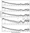 |
Fig. 1. Chandra/HETGS observations from 2001 binned at 0.03 Å. |
To investigate potential line variability, we calculated ratio spectra by comparing the high-flux state (ObsID 2093) to four lower-flux states (ObsIDs 2090, 2091, 2092, and 2094) that were observed within approximately one to three months of the high-flux state.
To account for the effect of continuum variation, we normalised the low-flux data to the high-flux state based on the average flux in the 9−14 Å band. The resulting ratio spectrum between ObsID 2090 and ObsID 2093 is presented in Fig. 2.
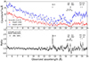 |
Fig. 2. Distinct spectral line variability are revealed by ratio spectrum in wavelength range of 5 − 20 Å. The top panel shows the low-flux state ObsID 2090 and high-flux state ObsID 2093 spectra binned to 0.1 Å. The bottom panel shows the low-flux state ObsID 2090 scaled up by a factor of 2.21 and the ratio spectrum defined by the low-flux state over the high-flux state ObsID 2093. |
To construct a continuous light curve, we combined RXTE/PCA and Chandra/HETGS data, as shown in Fig. 3. We converted the Chandra/HETGS fluxes to the equivalent RXTE 2−60 keV flux using WebPIMMS, assuming a power-law continuum and a Galactic absorption column density of 8.7 × 1020 cm−2 (Alloin et al. 1995). The converted flux levels are provided in Table 1. The Chandra observations analysed in this study are marked in red in Fig. 3 and are plotted at the midpoint of each exposure. Regarding long-term variability, we also include the observation taken in 2000 (ObsID 373) in order to illustrate the long-term timescale.
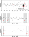 |
Fig. 3. RXTE light curve of NGC 3783 together with the epochs of six Chandra observations. In the top panel, the horizontal line represents the average flux level over 1.5 years of RXTE observations. The light grey shade bars represent the epochs of the Chandra observations. |
Observation log of NGC 3783 in 2000−2001 campaign.
3. Method
To investigate the spectral variability, we employed the tpho model (Rogantini et al. 2022) of SPEX (v3.08.01; Kaastra et al. 1996, 2024). Following Li et al. (2023), the initial unobscured SED is derived from the average broadband spectrum presented by Mehdipour et al. (2017) with no assumed changes in SED shape over time. The nine warm absorber components identified by Mao et al. (2019) were implemented within tpho, with their equilibrium properties serving as initial conditions. To capture the effects of long-term variability, we traced the evolution of each warm absorber component, extending sufficiently far back in time, guided by the up to weeks of RXTE monitoring preceding the Chandra observations are shown in Fig. 4.
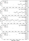 |
Fig. 4. RXTE light curve used as input for each tpho component calculation with the same starting data point from 1800 MJD. We show the part of the light curve within 14 days before the Chandra observation (red dot) corresponding to each component. The markers are similar to Fig. 3. The time resolution (tbin) in units of seconds was defined by the time difference between the Chandra observation and the last RXTE observation before it. |
Each component was exposed to the same unobscured SED, with light curves varying according to the observed data. This approach enabled us to assess how flux amplitude influences the resulting absorption spectra. The simulated transmissions were then cosmologically redshifted and convolved with the MEG response function. Finally, we derived the model ratio between low- and high-flux states from the simulated transmissions, with each state normalised separately to its respective continuum level.
4. Results
The ratio spectrum in Figure 2 reveals distinct features corresponding to the rest-frame wavelengths of the Ne IX resonance line (13.447 Å), the Fe UTA absorption complex (16−17 Å), the narrow O VII radiative recombination continuum (RRC at the O VII edge, 16.771 Å), the O VII absorption edge (16.771 Å), and the O VII/O VIII absorption lines (18.627 Å and 18.973 Å, respectively). As the Ne emission lines are relatively narrow, they are likely stable over time, appearing to deviate from unity due to the ratio spectrum’s normalisation against a variable continuum. The optical depths of the O VII Lyβ, O VIII Lyα, and Ne IX resonance lines are very large, which indicates that all of these absorption lines are saturated. In contrast, the Fe UTA absorption complex and the O VII edge (16 − 17.5 Å in the observed frame) exhibit significant variability, serving as the primary diagnostic indicators of warm absorber variation. By fitting the ratio spectrum with a combination of positive and negative Gaussian components, we determined a 10σ significance for Fe UTA variation, which is consistent with findings by Krongold et al. (2005).
Figure 5 demonstrates that the fifth component of transmission (which we refer to as component 5), with log ξ = 1.65 and column density = 0.5 × 1026 m−2, is the main contributor to the Fe UTA complex and O VII edge. The spectral variations observed in the ratio spectrum (Figure 2) reflect an increase in optical depth at the long-wavelength end of the Fe UTA and the O VII edge during the low-flux state, suggesting a response of the ionisation state of the warm absorber.
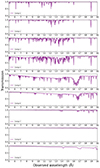 |
Fig. 5. Transmissions of the nine warm absorber components of NGC 3783 computed with the pion model based on the parameters listed in Mao et al. (2019). |
Figure 6 displays the results from the tpho calculations for component 5 and the best fit to the observed ratio of ObsID 2090 over 2093 within the local wavelength range of 15 − 18 Å. Panel a shows a clear transmission change from low-flux (red) to high-flux (blue) states at the same density, with the transmission ratio (black) revealing prominent peaks and dips exceeding 20% within the 16 − 17 Å wavelength range.
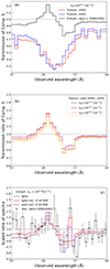 |
Fig. 6. Models from tpho for component 5 in the 15 − 18 Å binned with 0.1 Å. Panel a shows the transmission of component 5 in the high-flux state (blue) and low-flux state (red) and the transmission ratio (black) from the low-flux state over the high-flux state. Panel b shows the transmission ratio of component 5 as a function of increasing density. Panel c shows the observed ratio (black) was fitted well by the tpho model with a density of 1013.4 m−3 including the O VII RRC feature (red). The local scaling factor of 2.21 was calculated from the counts in the 9 − 14 Å range. |
Panel b of Figure 6 shows that calculations at lower densities (purple) produce weaker or negligible variations within the 16 − 17.5 Å band, which is attributed to longer recombination timescales and reduced variability in ionisation structure. In contrast, higher-density calculations (red and yellow lines) amplify the contrast between low- and high-flux states, with the greatest amplification occurring at a density of 1013.4 m−3, the current limit of our computational capabilities.
Panel c of Figure 6 demonstrates that a density of 1013.4 m−3 is optimal for reproducing the observed UTA and O VII edge variations, as suggested by the tpho calculations for component 5. Figure 2 displays a peak in the ratio spectrum corresponding to the narrow O VII RRC at 16.85 Å in the observed frame. To interpret this feature, we assumed that the RRC component remains constant over time, with the peak arising solely from continuum variation. This assumption is reasonable, as the RRC likely originates from the narrow line region, which is characterised by a low density (estimated around 1010 m−3, Davies et al. 2020) and thus has a recombination timescale of approximately one year (see Table 4 of Li et al. 2023). In panel c, the red line representing the model ratio under this assumption agrees well with the observed data. The green line showing the tpho calculation without adding the O VII RRC ratio gives a poorer fit. Additionally, we present the pion model calculation (purple), which closely matches the tpho results at a density of 1013.4 m−3 within the Fe UTA band. However, slight discrepancies are noted around the O VII edge band, with the pion model displaying a slightly lower continuum level than tpho. This suggests additional continuum absorption in the pion calculation, likely arising from oxygen within this wavelength range. We explore this aspect in greater detail in the discussion section.
In addition to component 5, component 6 might also partially contribute to the Fe UTA and O VII edge structure (see Fig. 5). However, our tpho calculations reveal that variations in component 6 are relatively minor, showing changes of less than 10%, especially when compared to the more substantial variability predicted for component 5.
To further constrain the density of component 5, we conducted a joint analysis of the ratio spectra from all four low-flux observations (ObsIDs 2090, 2091, 2092, and 2094) relative to ObsID 2093 within the 15 − 18 Å range. Figure 7 presents the ratio spectra (in black), fitted with the component 5 model (in green), the component 5 model including RRC (in red) with a density of 1013.4 m−3, and the pion model (in purple). Unlike ObsID 2090, the other three ObsIDs do not exhibit strong variation in ratio structure. Specifically, for ObsID 2094, the tpho model ratio for component 5 aligns well with the pion model, suggesting that the observed variations are within the expected range at this density level.
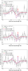 |
Fig. 7. Best fit of observation ratio with model ratio for groups of ObsID 2091/2093, ObsID 2092/2093, and ObsID 2094/2093 corresponding to the local scaling factor of 2.30, 1.87, and 1.66, respectively. The same approach was used as shown in Fig. 6. |
For component 5 (log ξ = 1.65), we performed a series of tpho calculations across a density range from 108 to 1015 m−3. For each density, we calculated a chi-square value by comparing the model predictions to the observed ratio spectra (Figure 8). Because the sampling of the input light curve for ObsID 2094 is sparse (2 × 10⁵ s), especially in the last two weeks, it cannot give a reliable constraint for densities ≥1012 m−3 for oxygen nor for densities ≥1010.3 m−3 for iron corresponding to the recombination timescale of 2 × 10⁵ s for that density, separately (see vertical dashed lines of Figure 9 and refer to Li et al. 2023). For the remaining observations, the sampling time is much shorter, of the order of 104 s (see Fig. 4), and we obtained reliable predictions for densities up to 1013.4 m−3. Again, for higher densities, the sampling uncertainties led to too high uncertainties in the predicted transmission. We combine the results for the three comparisons of Fig. 8 in Fig. 9. The density corresponding to the minimum chi-square value of 128.76, which is 1013.4 m−3, represents the best-fit solution confidently. At the 3σ confidence level, we found that the density is higher than 1012.3 m−3. The conservative lower limit by the tpho model calculation indicates that the assumption of photoionisation equilibrium (pion in the horizontal solid line with χ2 = 138) is less accurate than the tpho predictions at the 3.1σ confidence level (χ2 = 137). Additionally, Our lower limit is at least two orders of magnitude higher compared to the estimate based on photoionisation equilibrium by Krongold et al. (2005), who derived a density of > 1 × 10¹⁰ m−3.
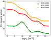 |
Fig. 8. Chi-square values computed from a comparison of observed spectral ratios with model ratios computed with the tpho model. |
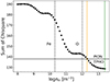 |
Fig. 9. Sum of chi-square values from Fig. 8 vs. density (black dots). The minimum chi-square value of 128.76 is obtained for a density of 1013.4 m−3 (green line). The chi-square value for fits with the pion model is shown as a solid horizontal line, which is higher than the tpho value at the 3σ confidence level (orange line). The vertical dashed lines indicate the densities of the outflow corresponding to a recombination time scale of 105 s for oxygen and iron. |
5. Discussion
Through our analysis of the extensive Chandra/HETGS data set from the 2001 NGC 3783 campaign, we identified significant spectral variability within the 16 − 17 Å range, with the most notable changes occurring on a monthly timescale. This finding indicates that the flux variation is likely driven by long-term fluctuations (on the order of months or more) that influence the plasma state of the warm absorber. Time-dependent photoionisation modelling using tpho and incorporating the RXTE light curve with a daily binning, suggests that the observed variability is predominantly attributable to component 5 of the warm absorber (log ξ = 1.65). This component requires a density of at least 2.0 × 10¹² m−3 to account for the variability, thus constraining its location to within 0.27 pc.
Our results confirm the flux-dependent features reported by Krongold et al. (2005). However, the density limits derived in our study are significantly higher than those presented in their work. This difference can likely be attributed to the advancements in our model, which employs the latest time-dependent photoionisation calculations and updated atomic data. Additionally, our findings are consistent with the density range reported by Gu et al. (2023), who also utilised the tpho model but employed a fundamentally different approach that focused solely on spectroscopic fitting of the time-averaged spectrum.
The soft excess reported by Netzer et al. (2003) and Krongold et al. (2005) could potentially introduce systematic uncertainties into our results, as the current tpho model does not account for changes in the SED. To assess the impact of the soft excess, we increased the flux in the 10 − 30 Å range by 20% and re-ran the tpho calculation for component 5. As shown in Figure 10, the soft excess has a negligible effect on the time variability of the Fe UTA and O edge within the relevant wavelength range, particularly in our fitting range.
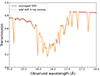 |
Fig. 10. Transmission of component 5 with the pion calculation by using different SED. The purple line indicates the averaged SED, and the orange curve denoted the SED adding soft X-ray excess in wavelength of 10 − 30 Å. |
Netzer et al. (2003) concluded that the observed changes in the underlying continuum were attributed to the appearance (high-flux state) and disappearance (low-flux state) of the soft excess component. This conclusion is consistent with the observations from ObsIDs 2093 and 2090, as shown in Fig. 1. The significant Fe UTA structure observed in ObsID 2093, following ObsID 2090, suggests that the Fe charge state has changed on a monthly timescale according to tpho calculations, allowing us to constrain the density of the low-ionisation component of the warm absorbers. Fig. 10 demonstrates that the soft X-ray excess does not significantly affect the Fe UTA feature, especially under the assumption of high density for the warm absorber component, as predicted by the pion model.
As illustrated in Figure 6, component 5 exhibits absorption features primarily from the Fe UTA and O VII edge at the relevant wavelengths. Due to their distinct recombination timescales–approximately 103 seconds for Fe and 105 seconds for O VII at a density of 1012 m−3–Fe and O VII respond differently to source variations, with Fe reacting to more rapid fluctuations while O VII primarily reflects longer-term changes. To fully separate the spectral contributions from Fe and O VII, a detailed analysis of spectral variations on hour- and day-level timescales would be ideal, though such data are not immediately available in this study. However, an estimate of their relative contributions to the observed spectral ratio variation can still be obtained. By setting the oxygen column density to zero in the tpho calculation, we isolated the Fe UTA feature (represented as the dashed line in Figure 11), and we compared it to the combined Fe and O VII calculation (shown as the solid line). The results suggest that Fe UTA absorption predominantly drives the variation in the 16 − 16.6 Å range, while the O VII edge contribution is secondary.
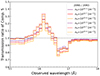 |
Fig. 11. Transmission ratio of component 5 with the tpho model for different densities in solid and dashed lines (including or excluding oxygen, respectively). |
The comparison between the tpho and pion models shown in panel c of Figure 6 reveals subtle differences between the out-of-equilibrium and equilibrium assumptions, particularly in the 16.7 − 17 Å range, where the O VII edge contributes. By calculating the ratio of the tpho to the pion transmission ratios, shown as the blue line in Figure 12, we observed that in the Fe UTA band, the tpho model with a density of 1013.4 m−3 matches closely with pion. However, in the 16.7 − 17 Å range, where the O VII edge impacts absorption, tpho shows a 10% difference from pion.
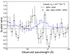 |
Fig. 12. Observation ratio is compared to the transmission ratio of component 5 with different assumptions. The observation ratio of ObsID 2090 to 2093 is illustrated with a black curve, and the transmission ratio of non-equilibrium (tpho) over equilibrium (pion) is represented by the blue line. |
Considering this, and noting the slight decrease in continuum absorption in the pion model in Figure 6, we hypothesise that in ObsIDs 2090 and 2093, Fe has likely reached equilibrium while oxygen has not. This is due to the fact that the recombination timescale for Fe (100 seconds at 1013.6 m−3) is considerably shorter than the light curve sampling interval, allowing Fe to reach equilibrium quickly (also refer to Figure 4). In contrast, oxygen, with a recombination timescale of approximately 104 s at the same density, aligns more closely with the sampling bin size, causing its response to lag behind the observed flux variations. Consequently, given the gaps between observations, oxygen could serve as an insightful diagnostic tool to probe higher-density plasmas, where recombination timescales more effectively reveal out-of-equilibrium effects (see Fig. 9). This further emphasises the importance of considering both density and recombination timescales when characterizing plasma conditions in variable environments.
The upper limit of the density nH, upp for an escaping wind is derived from the assumption that the outflowing velocity vout is larger than or equal to the escape velocity  . This yields
by substituting the escaping velocity into Eq. (1). The lower limit density nH of component 5 from our present tpho modelling is larger than nH, upp (see Figure 8 of Li et al. 2023), which indicates that the velocity of component 5 remains below the escape velocity. Therefore, this velocity discrepancy suggests that component 5 may be a failed wind that was unable to reach velocities sufficient to escape the gravitational pull of the SMBH and thus remains bound to the system.
Based on the density constraints shown in Figure 9, we could constrain the distance r of the low-ionisation warm absorber component using Eq. (1). Inserting log ξ = 1.65 and Lion = 6.36 × 1036 W (Mehdipour et al. 2017), at the 3σ confidence level, the distance of component 5 is limited to less than 0.27 pc. The derived distance is notably closer to the central SMBH than previous estimates, such as the ≤6 pc derived by Krongold et al. (2005). This closer proximity aligns well with the density values inferred from other variability studies, such as the upper bounds suggested by Behar et al. (2003) based on XMM-Newton grating spectra analysis. Furthermore, the finding of this location is consistent with the modelling by Chelouche & Netzer (2005), who predicted that hot X-ray absorbers likely originate from within 1 pc by analysing thermodynamic conditions in the outflowing structures.
Combining the results from the GRAVITY Collaboration (2021), the upper distance limit for component 5 (0.27 pc) is smaller than the coronal line region (0.4 pc) but larger than the hot dust (0.14 pc) and BLR (16 light-days) as measured by Br γ. This is consistent with the predicted scenario of a low-ionisation radiatively driven wind, which fails to escape and returns to the disc (Gallo et al. 2023).
This ‘failed wind’ component could provide a physical framework for interpreting various phenomenological components of AGNs (Giustini & Proga 2021). For instance, the inner failed wind component might offer a physical interpretation for key AGN features, such as the high-ionisation BLR, the obscuring material, and the X-ray corona. Additionally, the failed wind solutions describing the inner accretion and ejection flows of AGNs could help assess whether they significantly alter the physical and geometrical structure of the innermost accretion flow around highly accreting SMBHs.
In any model that predicts the launching mechanism and the impact of outflows on the surrounding medium, it is essential to determine the precise distance at which the outflow is launched. Time-dependent photoionisation modelling, which incorporates the variability of the warm absorber, offers an advantage in accurately determining the gas density. High-sensitivity, high-resolution calorimeters (such as Resolve on board XRISM, Tashiro et al. 2020, and X-IFU, prepared for the future Athena X-ray observatory, Barret et al. 2018) will provide significant advancements, especially in the study of variable warm absorbers and in determining their gas densities.
6. Conclusions
In this study, we revisited the unobscured-state spectrum of NGC 3783 using archival Chandra/HETGS data from the 2001 campaign. We investigated spectral variability over timescales of several months by comparing ratio spectra across varying flux levels. Significant changes were observed in the ratio spectrum over week-to-month timescales, which corresponds to a flux variation factor of 1.4 − 2. This variability, detected at a significance level greater than 10σ at maximum flux, points to notable response in the ionising continuum. To further explore these changes, we applied time-dependent photoionisation modelling with tpho (SPEX) and found that the low-ionisation component (log ξ = 1.65) exhibits a pronounced sensitivity to flux variations in the Fe UTA band. We constrained the density of this low-ionisation component to be higher than 1012.3 m−3 at the 3σ confidence level. This density places the location of the component within 0.27 pc of the central source. Our results suggest that this low-ionisation component may represent a failed wind candidate, as it lacks sufficient momentum to escape the gravitational influence of the SMBH and instead remains bound within the system. This finding contributes to a refined understanding of the dynamics and structure of AGN outflows in NGC 3783.
Acknowledgments
We thank the anonymous referee for his/her constructive comments. C.L. acknowledges support from Chinese Scholarship Council (CSC) and Leiden University/Leiden Observatory, as well as SRON. SRON is supported financially by NWO, the Netherlands Organization for Scientific Research. C.L. thanks Elisa Costantini for the discussions of distance scale of outflowing wind.
References
- Alloin, D., Santos-Lleo, M., Peterson, B. M., et al. 1995, A&A, 293, 293 [NASA ADS] [Google Scholar]
- Ballhausen, R., Kallman, T. R., Gu, L., & Paerels, F. 2023, ApJ, 956, 65 [NASA ADS] [CrossRef] [Google Scholar]
- Barret, D., Lam Trong, T., den Herder, J.-W., et al. 2018, SPIE Conf. Ser., 10699, 106991G [Google Scholar]
- Behar, E., Sako, M., & Kahn, S. M. 2001, ApJ, 563, 497 [NASA ADS] [CrossRef] [Google Scholar]
- Behar, E., Rasmussen, A. P., Blustin, A. J., et al. 2003, ApJ, 598, 232 [Google Scholar]
- Bentz, M. C., Williams, P. R., Street, R., et al. 2021, ApJ, 920, 112 [NASA ADS] [CrossRef] [Google Scholar]
- Blustin, A. J., Branduardi-Raymont, G., Behar, E., et al. 2002, A&A, 392, 453 [NASA ADS] [CrossRef] [EDP Sciences] [Google Scholar]
- Chelouche, D., & Netzer, H. 2005, ApJ, 625, 95 [NASA ADS] [CrossRef] [Google Scholar]
- Davies, R. I., Burtscher, L., Rosario, D., et al. 2015, ApJ, 806, 127 [Google Scholar]
- Davies, R., Baron, D., Shimizu, T., et al. 2020, MNRAS, 498, 4150 [Google Scholar]
- Gabel, J. R., Kraemer, S. B., Crenshaw, D. M., et al. 2005, ApJ, 631, 741 [NASA ADS] [CrossRef] [Google Scholar]
- Gallo, L. C., Miller, J. M., & Costantini, E. 2023, ArXiv e-prints [arXiv:2302.10930] [Google Scholar]
- Giustini, M., & Proga, D. 2021, IAU Symp., 356, 82 [NASA ADS] [Google Scholar]
- GRAVITY Collaboration (Amorim, A., et al.) 2021, A&A, 648, A117 [NASA ADS] [CrossRef] [EDP Sciences] [Google Scholar]
- Gu, L., Kaastra, J., Rogantini, D., et al. 2023, A&A, 679, A43 [NASA ADS] [CrossRef] [EDP Sciences] [Google Scholar]
- Juráňnová, A., Costantini, E., & Uttley, P. 2022, MNRAS, 510, 4225 [CrossRef] [Google Scholar]
- Kaastra, J. S., Mewe, R., & Nieuwenhuijzen, H. 1996, in UV and X-ray Spectroscopy of Astrophysical and Laboratory Plasmas, eds. K. Yamashita, & T. Watanabe, 411 [Google Scholar]
- Kaastra, J. S., Detmers, R. G., Mehdipour, M., et al. 2012, A&A, 539, A117 [NASA ADS] [CrossRef] [EDP Sciences] [Google Scholar]
- Kaastra, J. S., Mehdipour, M., Behar, E., et al. 2018, A&A, 619, A112 [NASA ADS] [CrossRef] [EDP Sciences] [Google Scholar]
- Kaastra, J. S., Raassen, A. J. J., de Plaa, J., & Gu, L. 2024, https://doi.org/10.5281/zenodo.7037609 [Google Scholar]
- Kaspi, S., Brandt, W. N., George, I. M., et al. 2002, ApJ, 574, 643 [NASA ADS] [CrossRef] [Google Scholar]
- Krolik, J. H., McKee, C. F., & Tarter, C. B. 1981, ApJ, 249, 422 [NASA ADS] [CrossRef] [Google Scholar]
- Krongold, Y., Nicastro, F., Brickhouse, N. S., et al. 2003, ApJ, 597, 832 [NASA ADS] [CrossRef] [Google Scholar]
- Krongold, Y., Nicastro, F., Brickhouse, N. S., Elvis, M., & Mathur, S. 2005, ApJ, 622, 842 [NASA ADS] [CrossRef] [Google Scholar]
- Li, C., Kaastra, J. S., Gu, L., & Mehdipour, M. 2023, A&A, 680, A44 [NASA ADS] [CrossRef] [EDP Sciences] [Google Scholar]
- Mao, J., Kaastra, J. S., Mehdipour, M., et al. 2017, A&A, 607, A100 [NASA ADS] [CrossRef] [EDP Sciences] [Google Scholar]
- Mao, J., Mehdipour, M., Kaastra, J. S., et al. 2019, A&A, 621, A99 [NASA ADS] [CrossRef] [EDP Sciences] [Google Scholar]
- Mehdipour, M., Kaastra, J. S., Kriss, G. A., et al. 2017, A&A, 607, A28 [NASA ADS] [CrossRef] [EDP Sciences] [Google Scholar]
- Netzer, H., Kaspi, S., Behar, E., et al. 2003, ApJ, 599, 933 [NASA ADS] [CrossRef] [Google Scholar]
- Rogantini, D., Mehdipour, M., Kaastra, J., et al. 2022, ApJ, 940, 122 [NASA ADS] [CrossRef] [Google Scholar]
- Sadaula, D. R., Bautista, M. A., García, J. A., & Kallman, T. R. 2023, ApJ, 946, 93 [NASA ADS] [CrossRef] [Google Scholar]
- Silva, C. V., Uttley, P., & Costantini, E. 2016, A&A, 596, A79 [NASA ADS] [CrossRef] [EDP Sciences] [Google Scholar]
- Tarter, C. B., Tucker, W. H., & Salpeter, E. E. 1969, ApJ, 156, 943 [Google Scholar]
- Tashiro, M., Maejima, H., Toda, K., et al. 2020, SPIE Conf. Ser., 11444, 1144422 [Google Scholar]
- Theureau, G., Bottinelli, L., Coudreau-Durand, N., et al. 1998, A&AS, 130, 333 [NASA ADS] [CrossRef] [EDP Sciences] [Google Scholar]
All Tables
All Figures
|
Fig. 1. Chandra/HETGS observations from 2001 binned at 0.03 Å. |
| In the text | |
|
Fig. 2. Distinct spectral line variability are revealed by ratio spectrum in wavelength range of 5 − 20 Å. The top panel shows the low-flux state ObsID 2090 and high-flux state ObsID 2093 spectra binned to 0.1 Å. The bottom panel shows the low-flux state ObsID 2090 scaled up by a factor of 2.21 and the ratio spectrum defined by the low-flux state over the high-flux state ObsID 2093. |
| In the text | |
|
Fig. 3. RXTE light curve of NGC 3783 together with the epochs of six Chandra observations. In the top panel, the horizontal line represents the average flux level over 1.5 years of RXTE observations. The light grey shade bars represent the epochs of the Chandra observations. |
| In the text | |
|
Fig. 4. RXTE light curve used as input for each tpho component calculation with the same starting data point from 1800 MJD. We show the part of the light curve within 14 days before the Chandra observation (red dot) corresponding to each component. The markers are similar to Fig. 3. The time resolution (tbin) in units of seconds was defined by the time difference between the Chandra observation and the last RXTE observation before it. |
| In the text | |
|
Fig. 5. Transmissions of the nine warm absorber components of NGC 3783 computed with the pion model based on the parameters listed in Mao et al. (2019). |
| In the text | |
|
Fig. 6. Models from tpho for component 5 in the 15 − 18 Å binned with 0.1 Å. Panel a shows the transmission of component 5 in the high-flux state (blue) and low-flux state (red) and the transmission ratio (black) from the low-flux state over the high-flux state. Panel b shows the transmission ratio of component 5 as a function of increasing density. Panel c shows the observed ratio (black) was fitted well by the tpho model with a density of 1013.4 m−3 including the O VII RRC feature (red). The local scaling factor of 2.21 was calculated from the counts in the 9 − 14 Å range. |
| In the text | |
|
Fig. 7. Best fit of observation ratio with model ratio for groups of ObsID 2091/2093, ObsID 2092/2093, and ObsID 2094/2093 corresponding to the local scaling factor of 2.30, 1.87, and 1.66, respectively. The same approach was used as shown in Fig. 6. |
| In the text | |
|
Fig. 8. Chi-square values computed from a comparison of observed spectral ratios with model ratios computed with the tpho model. |
| In the text | |
|
Fig. 9. Sum of chi-square values from Fig. 8 vs. density (black dots). The minimum chi-square value of 128.76 is obtained for a density of 1013.4 m−3 (green line). The chi-square value for fits with the pion model is shown as a solid horizontal line, which is higher than the tpho value at the 3σ confidence level (orange line). The vertical dashed lines indicate the densities of the outflow corresponding to a recombination time scale of 105 s for oxygen and iron. |
| In the text | |
|
Fig. 10. Transmission of component 5 with the pion calculation by using different SED. The purple line indicates the averaged SED, and the orange curve denoted the SED adding soft X-ray excess in wavelength of 10 − 30 Å. |
| In the text | |
|
Fig. 11. Transmission ratio of component 5 with the tpho model for different densities in solid and dashed lines (including or excluding oxygen, respectively). |
| In the text | |
|
Fig. 12. Observation ratio is compared to the transmission ratio of component 5 with different assumptions. The observation ratio of ObsID 2090 to 2093 is illustrated with a black curve, and the transmission ratio of non-equilibrium (tpho) over equilibrium (pion) is represented by the blue line. |
| In the text | |
Current usage metrics show cumulative count of Article Views (full-text article views including HTML views, PDF and ePub downloads, according to the available data) and Abstracts Views on Vision4Press platform.
Data correspond to usage on the plateform after 2015. The current usage metrics is available 48-96 hours after online publication and is updated daily on week days.
Initial download of the metrics may take a while.