| Issue |
A&A
Volume 678, October 2023
|
|
|---|---|---|
| Article Number | A173 | |
| Number of page(s) | 15 | |
| Section | Extragalactic astronomy | |
| DOI | https://doi.org/10.1051/0004-6361/202346981 | |
| Published online | 18 October 2023 | |
An extremely metal-poor star complex in the reionization era: Approaching Population III stars with JWST⋆
1
INAF – OAS, Osservatorio di Astrofisica e Scienza dello Spazio di Bologna, Via Gobetti 93/3, 40129 Bologna, Italy
e-mail: This email address is being protected from spambots. You need JavaScript enabled to view it.
2
Dipartimento di Fisica, Università degli Studi di Milano, Via Celoria 16, 20133 Milano, Italy
3
INAF – Osservatorio Astronomico di Roma, Via Frascati 33, 00078 Monteporzio Catone, Rome, Italy
4
Dipartimento di Fisica e Scienze della Terra, Università degli Studi di Ferrara, Via Saragat 1, 44122 Ferrara, Italy
5
INAF – IASF Milano, Via A. Corti 12, 20133 Milano, Italy
6
University of Ljubljana, Department of Mathematics and Physics, Jadranska ulica 19, 1000 Ljubljana, Slovenia
7
Department of Physics and Astronomy, University of California Davis, 1 Shields Avenue, Davis, CA 95616, USA
8
Department of Astronomy, Oskar Klein Centre, Stockholm University, AlbaNova University Centre, 106 91 Stockholm, Sweden
9
NSF’s National Optical-Infrared Astronomy Research Laboratory, 950 N. Cherry Ave., Tucson, AZ 85719, USA
10
Max Planck Institut für Astrophysik, Karl-Schwarzschild-Straße 1, 85748 Garching bei München, Germany
11
INAF Osservatorio Astronomico di Padova, Vicolo dell’Osservatorio 5, 35122 Padova, Italy
12
NRC Herzberg, 5071 West Saanich Rd, Victoria, BC V9E 2E7, Canada
13
Département d’Astronomie, Université de Genève, Chemin Pegasi 51, 1290 Versoix, Switzerland
14
European Southern Observatory, Alonso de Córdova 3107, Casilla 19, Santiago 19001, Chile
15
Dipartimento di Fisica e Astronomia, Università degli Studi di Padova, Vicolo dell’Osservatorio 3, 35122 Padova, Italy
16
European Southern Observatory, Karl-Schwarzschild-Strasse 2, 85748 Garching bei München, Germany
17
Kapteyn Astronomical Institute, University of Groningen, PO Box 800 9700 AV Groningen, The Netherlands
18
Department of Astronomy, University of Maryland, College Park 20742, USA
19
Space Telescope Science Institute (STScI), 3700 San Martin Drive, Baltimore, MD 21218, USA
20
Dipartimento di Fisica “E.R. Caianiello”, Università Degli Studi di Salerno, Via Giovanni Paolo II, 84084 Fisciano, SA, Italy
21
INAF – Osservatorio Astronomico di Capodimonte, Via Moiariello 16, 80131 Napoli, Italy
22
Cosmic Dawn Center (DAWN), Copenhagen, Denmark
23
Niels Bohr Institute, University of Copenhagen, Jagtvej 128, 2200 Copenhagen N, Denmark
24
Institute for Computational Astrophysics and Department of Astronomy & Physics, Saint Mary’s University, 923 Robie Street, Halifax, NS B3H 3C3, Canada
25
Technical University of Munich, Department of Physics, James-Franck-Straße 1, 85748 Garching, Germany
26
Centro de Astrobiología (CAB), CSIC-INTA, Ctra. de Ajalvir km 4, Torrejòn de Ardoz, 28850 Madrid, Spain
27
INAF-Trieste Astronomical Observatory, Via Bazzoni 2, 34124 Trieste, Italy
Received:
23
May
2023
Accepted:
28
July
2023
Abstract
We present JWST/Near Infrared Spectrograph (NIRSpec) integral field spectroscopy (IFS) of a lensed Population III candidate stellar complex (dubbed Lensed And Pristine 1, LAP1), with a lensing-corrected stellar mass of ≲104 M⊙ and an absolute luminosity of MUV > −11.2 (mUV > 35.6), confirmed at redshift 6.639 ± 0.004. The system is strongly amplified (μ ≳ 100) by straddling a critical line of the Hubble Frontier Field galaxy cluster MACS J0416. Although the stellar continuum is currently not detected in the Hubble and JWST/Near Infrared Camera (NIRCam) and Near Infrared Imager and Slitless Spectrograph (NIRISS) imaging, arclet-like shapes of Lyman and Balmer lines, Lyα, Hγ, Hβ and Hα are detected with NIRSpec IFS with signal-to-noise ratios (S/N) of approximately 5 − 13 and large equivalent widths (> 300 − 2000 Å), along with a remarkably weak [O III]λλ4959, 5007 at S/N ≃ 4. LAP1 shows a large ionizing photon production efficiency, log(ξion[erg Hz−1]) > 26. From the metallicity indexes R23 = ([O III] + [O II])/Hβ ≲ 0.74 and R3 = ([O III]/Hβ) = 0.55 ± 0.14, we derive an oxygen abundance of 12 + log(O/H)≲6.3. Intriguingly, the Hα emission is also measured in mirrored subcomponents where no [O III] is detected, providing even more stringent upper limits on the metallicity if in situ star formation is ongoing in this region (12 + log(O/H) < 6). The formal stellar mass limit of the subcomponents would correspond to ∼103 M⊙ or MUV fainter than −10. Alternatively, this metal-free, pure line-emitting region could be the first case of a fluorescing H I gas region induced by transverse escaping ionizing radiation from a nearby star complex. The presence of large equivalent-width hydrogen lines and the deficiency of metal lines in such a small region make LAP1 the most metal-poor star-forming region currently known in the reionization era and a promising site that may host isolated, pristine stars.
Key words: stars: Population III / galaxies: high-redshift / galaxies: star formation / gravitational lensing: strong
Based on observations collected with the James Webb Space Telescope (JWST) and Hubble Space Telescope (HST). These observations are associated with JWST GO program n.1908 (PI: E. Vanzella) and GTO n.1208 (CANUCS, PI: C. Willot).
© The Authors 2023
 Open Access article, published by EDP Sciences, under the terms of the Creative Commons Attribution License (https://creativecommons.org/licenses/by/4.0), which permits unrestricted use, distribution, and reproduction in any medium, provided the original work is properly cited.
This article is published in open access under the Subscribe to Open model. This email address is being protected from spambots. You need JavaScript enabled to view it. to support open access publication.
1. Introduction
With the advent of JWST, the search for metal-free, population III (PopIII) sources is now entering a golden epoch. Although no direct observations of PopIII stars have been made to date, their existence is supported by cosmological simulations (Abel et al. 2002; Bromm et al. 2002; Maio et al. 2010; Hirano et al. 2014; Park et al. 2021; Yajima et al. 2023; Klessen & Glover 2023, and references therein) and the observation of extremely metal-poor halo stars, which are believed to be enriched by metals produced in PopIII stars (e.g., Salvadori et al. 2007; Hartwig et al. 2018; Vanni et al. 2023).
Many recent papers have proposed key diagnostics designed to help identify these elusive pristine stars. The expected presence or deficit of emission lines in PopIII sources coupled with the underlying shape of the stellar continuum affects the colors of key photometric bands, which can now be easily probed in the ultraviolet/optical rest frame up to z ∼ 15 with JWST/NIRCAM and MIRI (e.g., see Trussler et al. 2023 and references therein). Even more informative is the direct access to ultraviolet and optical spectral features in the same early epochs (e.g., JWST/NIRSpec and/or MIRI), which can be used to derive rest-frame equivalent widths (EW0) and key line ratios (e.g., Nakajima et al. 2022, 2023; Cameron et al. 2023; Sanders et al. 2023). In particular, the presence of prominent helium (EW0 > 20 Å rest-frame) and Balmer (EW0 > 1000 Å) emission lines and Lyα (if not significantly attenuated by the IGM, EW0 > 1000 Å) and a deficit of metal lines provide support to the conclusion of very metal-poor conditions (Nakajima et al. 2022, see also Katz et al. 2023; Inoue 2011; Zackrisson et al. 2011; Schaerer 2002, 2003). However, despite the unprecedented capabilities of JWST, identifying PopIII stars remains challenging. In particular, a pocket of stars forming in pristine gas conditions at early epochs (either in isolation or as a metal-unpolluted satellite of a PopII galaxy) is expected to be out of reach, even given the sensitivity of the JWST. As a straightforward example, a star complex of PopIII stars at z = 7 with a stellar mass of 103, 4, 5 M⊙ corresponds an observed 1500 Å ultraviolet magnitude of 37.6, 35.1, 32.6 (assuming all stars have the same mass of 100 M⊙ and age ≲3 Myr for simplicity; Windhorst et al. 2018). The expected EW0 for the He IIλ1640 line in these complexes would span the interval 20 − 100 Å in the rest-frame (Nakajima & Maiolino 2022), which corresponds to fluxes of lower than 5 × 10⁻²⁰ erg s−1 cm−2. The strength of He IIλ1640 may be significantly affected by stochastic IMF sampling, which increases the variance of the emerging line flux, or be lowered by a factor of 10 or more if aging, different star formation rates (SFRs), or PopIII and PopII mixing are considered (Maio et al. 2016; Mas-Ribas et al. 2016; Katz et al. 2023; Vikaeus et al. 2022)1. These emission line flux and continuum levels also require a significant investment of time for JWST (e.g., at 2 μm a signal-to-noise ratio of S/N = 10 for a point-like source with line flux ≃4 × 10⁻¹⁹ erg s−1 cm−2 can be achieved with an integration time of 100 000 s, for R = 1000; Jakobsen et al. 2022).
In principle, the detection of more massive systems (e.g., 105 − 6 M⊙) purely composed of PopIII stars is possible with JWST. Indeed, detailed calculations at z = 8 by Trussler et al. (2023), adopting different IMFs for a 106 M⊙ PopIII complex, produce more accessible line fluxes (He IIλ1640) and magnitudes. In the most favorable conditions (e.g., adopting the Kroupa IMF used by these latter authors with a characteristic mass of stars of 100 M⊙), a few tens of hours of integration time with JWST/NIRSpec or NIRCam slitless spectroscopy are needed to reach a 5σ detection of the helium line, or a few hours with NIRCam if the source is imaged immediately after an instantaneous starburst. The exposure time diverges to hundreds of hours if the characteristic stellar mass decreases to 10 M⊙ or lower (see Trussler et al. 2023, for more details). Therefore, an integration time of dozens of hours would still be required, and the number density of such high-mass objects is still unknown and likely very low (Klessen & Glover 2023; Vikaeus et al. 2022). A mixture of PopII and PopIII components has been postulated (e.g., Venditti et al. 2023), with spectral features that reflect such a hybrid condition (Sarmento et al. 2018, 2019). However, even though these systems would produce accessible fluxes, the signature emerging from the pockets of pristine gas in the metal-enriched galaxy would be diluted or misinterpreted if insufficient angular resolution (spatial contrast) is available. Sources showing He IIλ1640 emission have already emerged at z ≃ 8 from initial JWST data, but further investigation is needed to better locate and characterize the region emitting such hard photons (Wang et al. 2022, see also the controversial case at z = 6.6, dubbed CR7; Sobral et al. 2019; Shibuya et al. 2018), and we must also note that even metal-enriched star-forming regions with SFR < 1 M⊙ yr−1 can show elevated He IIλ1640 equivalent width due to IMF sampling issues (e.g., Vikaeus et al. 2020; see also Shirazi & Brinchmann 2012; Senchyna et al. 2020, 2021; Schaerer et al. 2019; Kehrig et al. 2018; Bik et al. 2018, who report additional production mechanisms and sources of He IIλ1640 line emission, such as high-mass X-ray binaries, shocks, or very massive stars).
Because of these limitations, gravitational lensing has been identified as a promising tool with which to investigate pristine stars (Rydberg et al. 2013; Zackrisson et al. 2015; Vikaeus et al. 2022; Vanzella et al. 2020). In particular, lensing magnification increases (1) the spatial contrast and (2) the S/N of the observed features, with a caveat being the limited accessible volume as the magnification increases. Therefore, if the identification of extremely metal-poor conditions is restricted to very small spatial scales (e.g., before the targeted region is polluted by any previous or nearby/concurrent star formation event), the required large spatial contrast in such studies becomes relevant. Indeed, the fact that an isolated stellar complex or cluster of extremely metal-poor (EMP) or metal-free stars is expected to be found in isolation means that special observational conditions are required (Katz et al. 2023).
Vanzella et al. (2020) reported the identification of a Lyα-arclet at redshift z = 6.63 straddling a critical line, with no evident detection of a stellar counterpart in deep Hubble Frontier Fields (HFF) images of the galaxy cluster MACS J0416 (Lotz et al. 2017). The Lyα emission was detected at S/N = 17 from deep MUSE observations (Vanzella et al. 2020, 2021), with a flux of (4.4 ± 0.25)×10−18 erg s−1 cm−2 and an equivalent width likely larger than 500 Å rest-frame (or 1000 Å if the intergalactic medium (IGM) attenuates 50% of the line). The undetected stellar counterpart and the large amplification lead to an estimated stellar mass of ≃104 M⊙. Though possibly rare at these redshifts (but still expected down to z ∼ 3 − 5; Tornatore et al. 2007; Bromm 2013; Pallottini et al. 2014; Liu & Bromm 2020), large equivalent widths indicate the possible presence of extremely metal-poor or even PopIII stars, making this source an ideal target for JWST (Gardner et al. 2023; Rigby et al. 2023). Moreover, at z = 6.64, all the Balmer and the most prominent metal lines (e.g., [O III]λλ4959, 5007) can be captured in a single observation with the JWST/NIRSpec prism observing mode (Jakobsen et al. 2022; Ferruit et al. 2022; Böker et al. 2023). Here, we present JWST/NIRSpec prism integral field spectroscopy observations of a similarly exotic source, covering the rest-frame spectral range from Lyα to Hα, in addition to JWST/(NIRCam + NIRISS) imaging.
Throughout this paper, we assume a flat cosmology with ΩM = 0.3, ΩΛ = 0.7, and H0 = 70 km s−1 Mpc−1. All magnitudes are given in the AB system (Oke & Gunn 1983): mAB = 23.9 − 2.5log(fν/μJy).
2. JWST and HST imaging: Still an undetected source
JWST/NIRCam and JWST/NIRISS observations were acquired on January 2023, as part of the CAnadian NIRISS Unbiased Cluster Survey: CANUCS (Willott et al. 2022). The galaxy cluster MACS J0416 was observed in eight NIRCam filters covering the spectral range from 0.8 μm to 5 μm (F090W, F115W, F150W, F200W, F277W, F356W, F410M, F444W) and with an integration time of 6400 s per band. JWST/NIRISS imaging was also acquired as part of the pre-imaging for slitless spectroscopy in the F115W, F150W, and F200W bands for an integration time of 2280 s per band. The images were processed using a combination of the STScI JWST pipeline v1.8.4 with CRDS context jwst_1027.pmap and GRIZLI v1.7.8 (Brammer et al. 2022). A more detailed description of the CANUCS imaging processing will be presented in Martis et al. (in prep.). The magnitude limits for point sources at 5σ are 29.4 and 29.1 in the F150W band for JWST/NIRCam and JWST/NIRISS, respectively. Hubble Frontier Fields data in the F435W, F606W, F814W, F105W, F125W, F140W, and F160W bands are also included in the set of images used in this work, all of them with a typical 5σ magnitude limit for point sources of ≃29 (Lotz et al. 2017).
Figure 1 shows the stacked images centered at the coordinates of the Lyα arclet, which is hereafter referred to as LAP1 (Lensed And Pristine 1). Remarkably, and similarly to what is shown by Vanzella et al. (2020), there is no evidence of stellar counterparts in the proximity of the arclet in any of the image sets, that is, of HST, JWST/NIRcam, or JWST/NIRISS, either in the deep stacked image – which collects F115W, F150W, and F200W (after combining NIRCam and NIRISS) probing the 2000 Å rest-frame – or in the redder bands (λ > 2 μm), F277W, F356W, F410M, and F444W, which probe the optical 4000 Å rest-frame. The deep stacked ultraviolet and optical images provide lower limits of mUV and mopt ≃30.4 at 2σ (≃31 at 1σ), when measuring the flux with the A-PHOT tool (Merlin et al. 2019) in an elliptical aperture that includes the full arclet shape. The magnitude limits are reported in Table 1 and are used in Sect. 5 to constrain the limits on the equivalent widths of the emission lines and the intrinsic luminosity. The delensed properties of LAP1 are reported in Sect. 4.
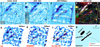 |
Fig. 1. Photometric and spectroscopic observations of LAP1. Hubble Frontier Fields (Lotz et al. 2017) and JWST NIRISS NIRCam imaging from the CANUCS GTO program (Willott et al. 2022). From top left to bottom right: (1) the combined HST F435W and F606W image probing λ < 915 Å at z = 6.639. The black arrow indicates the presence of a foreground object, which is nevertheless not significantly contaminating the extracted spectrum of LAP1; (2) the 11 stacked bands from JWST/NIRCam and NIRISS, as labeled in the bottom left (white and cyan labeled filters indicate NIRCam and NIRISS, respectively); (3) the median collapse of the entire NIRSpec datacube spanning the range 0.7 − 5.2 μm (black circles indicate sources visible in the JWST and HST imaging); (4) the color composite image with the three channels blue, green, and red as indicated in the legend on the left (we note that the red channel shows the 6 stacked bands F115W, F150W, and F200W combined from NIRISS and NIRCam). The white square marks the NIRSpec FoV. The yellow circles mark the same objects as in panel 3 and the green contour outlines the 3σ Lyα from VLT/MUSE; (5)–(7) show the Lyα, [O III]λ5007, and the sum Hγ + Hβ + Hα, with the critical line (in black) and the positions of the two B1,2 components (marked with red circles), respectively; (8) shows the masks used to extract the spectra from the sources described in the text. The elongated red contour of 2.3″ × 0.2″ outlines the aperture used to extract the spectrum of the arclet (LAP1), defined on the combined image of the Balmer lines (see Appendix B), while the ellipse indicates the aperture used to extract the spectrum shown in Fig. A.2 and the magnitudes of Source 1 (z = 2.41; see Appendix A). All panels have the same scale, indicated in panel 8. The angular size of the single spaxel and the PSF at 5 μm are reported in the bottom-right inset of panel 8. |
Observed and derived properties of LAP1.
Remarkably, despite the absence of any stellar counterpart, the JWST/NIRSpec observations reveal four emission lines, Lyα, Hγ, Hβ, [O III]λλ4959, 5007 and Hα, which follow the arclet-like shape already outlined by the previous VLT/MUSE Lyα emission at z = 6.64.
3. JWST NIRSpec/IFU observations
JWST/NIRSpec integral field unit (IFU) observations were performed on October 16 − 17, 2022, as part of five pointings targeting strongly lensed globular cluster precursors and candidate population III stellar complexes at redshift z = 6 − 7 (PI: Vanzella, prog. id 1908). In particular, four out of five pointings will cover a structure of tiny star-forming regions and proto-globulars at z = 6.14 (Vanzella et al. 2019, 2021; Calura et al. 2021) for a total integration time of ≃18 h (currently scheduled for Summer 2023). One out of five pointings was devoted to LAP1 at z = 6.64. Here we present observations of LAP1, which focus on an extremely faint candidate PopIII star complex discovered by Vanzella et al. (2020). These provide a total integration time of 6.19 h (including overheads) split into eight independent acquisitions of 2115.4 s each, for a net integration time on target of 4.7 h. The small (0.25″ extent) dithering cycling over eight points was applied to each acquisition.
3.1. Data reduction
We reduced the NIRSpec/IFU raw data using the STScI pipeline (version 1.9.5). The software version and the Calibration Reference Data System (CRDS) context are 11.16.20 and jwst_1062.pmap, respectively. The raw data (i.e., uncal exposures) were processed through three stages. In summary, Stage 1 is common to all the JWST instruments and corrects for detector-related issues (e.g., bias and dark subtraction, pixel saturation and deviation from linearity, and cosmic-ray flagging). Stage 2 converts the coordinates from the detector plane to sky coordinates and implements critical steps such as background subtraction, flat–field correction2, and flux and wavelength calibration. Also, intermediate datacubes associated with the single dithers are produced during this stage. The third and last stage combines the eight calibrated dithers into the final datacube.
We ran the three stages using the default parameters. We carefully inspected the intermediate products for each step. In particular, we did not find any significant vertical pattern associated with correlated noise (e.g., 1/f noise) in the count-rate images (i.e., rate files) produced after the first stage, as discussed by other works using NIRSpec/IFU (e.g., Marshall et al. 2023; Übler et al. 2023), and therefore we did not apply any correction outside the pipeline before running Stage 2. Moreover, we did not perform any background subtraction inside the pipeline, but used an independent procedure as described in Appendix A. Finally, we ran the Outlier Detection Step in Stage 3, which is meant to remove possible cosmic rays not recognized in the Jump Step of Stage 1 by comparing the single exposures. Other studies have shown that this step can lead to false-positive cosmic rays corresponding to bright sources in dithered exposures (i.e., quasars, see Cresci et al. 2023; Marshall et al. 2023; Perna et al. 2023), and therefore skipping this step is often recommended (see also Böker et al. 2023). However, by comparing the products obtained by applying and skipping the Outlier Detection procedure, we found that spurious cosmic rays are not produced at the location of the sources, which is likely due to the low flux regime of our targets. We verified that the application of this step with the default parameters works as expected, removing several spikes affecting our dataset. The final calibrated datacube is obtained after completing this three-stage data processing. We used the default spatial scale of 0.1″ for each spaxel.
Additional post-processing was performed on the reduced datacube. This includes background subtraction, the removal of outliers, and the computation of the error spectrum. In addition, cross-checks on the flux calibration were performed using JWST NIRCam, NIRISS, and Hubble photometry on sources lying in the same field of view (see Appendix A for more details). Finally, the detected sources in the reduced, post-processed, and collapsed datacube were aligned to the JWST/NIRCam counterparts by applying a rigid shift on right ascension (RA) and declination (Dec; see the sources marked with circles in Fig. 1).
3.2. Prominence of Balmer and deficit of metals lines
As discussed in Vanzella et al. (2020), the arclet was detected only in Lyα emission, without showing any significant stellar-continuum counterparts. The faintness of this object is also confirmed by the JWST imaging as reported in Sect. 2. However, the JWST spectroscopic data provide a wealth of unique information that is key to the physical interpretation of the source.
The Hα, Hβ, and Hγ emission lines emerge at the mean redshift z = 6.639 with a standard deviation of 0.004, resembling the same arclet-like orientation initially reported by Vanzella et al. (2020)3. In addition to Lyα, the Balmer lines Hγ, Hβ, and Hα are detected, along with a remarkably faint [O III]λλ4959, 5007. The arclet is considerably thin and appears not resolved along the radial direction4. We defined an elongated aperture using the stacked two-dimensional images of the emerging Balmer lines. In particular, the aperture extends 2.3″ along the arclet (tangential direction) and ≃0.2″ perpendicularly (radial direction), as outlined in Fig. 1 and nearly marks the 3σ contour of the arclet in the stacked image.
Figure 2 shows the one-dimensional spectrum of LAP1 and the line fluxes and errors are reported in Table 1. Hydrogen lines Lyα, Hγ, Hβ, and Hα are detected with S/N spanning the range 5 − 13 with unconstrained velocity widths, all of them consistent with the prism spectral resolution. The low spectral resolution provided by the prism mode R = 30(300) at λ = 1(5) μm corresponds to dv ≃ 10 000(1000) km s−1 and prevents us from measuring a velocity offset among the spectral features. The line ratios Hα/Hβ and Hβ/Hγ are consistent within the uncertainties with the case B recombination, corresponding to Hα/Hβ ≃ 2.8 and Hβ/Hγ ≃ 2.1 (e.g., Osterbrock 1989), implying very little or no dust attenuation. Under the same case B assumption, the expected Lyα/Hα is 8.7, suggesting that nearly half of the Lyα line is attenuated by the IGM (after neglecting any additional internal absorption or geometrical effect). Remarkably, the extracted spectrum from LAP1 shows [O III]λ5007 emission that is significantly fainter than that of Hβ, with [O III]λ5007/Hβ ≃ 0.55. It is worth noting that such a deficit of oxygen emission compared to the Balmer lines is in opposition to the strong optical oxygen emission recently observed at z > 5 − 6 with JWST, in which large equivalent widths of [O III] (> 1000 Å rest-frame) showing [O III]λ5007/Hβ ≫ 1 are commonly observed (e.g., Matthee et al. 2023; see also Withers et al. 2023; Rinaldi et al. 2023; Williams et al. 2023; Endsley et al. 2021; Boyett et al. 2022; Castellano et al. 2017; De Barros et al. 2019).
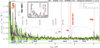 |
Fig. 2. One-dimensional NIRSpec spectrum of LAP1 (black line) extracted from the elongated aperture (“Arclet”) shown in panel 8 of Fig. 1. The most relevant lines, detected with S/N > 4, are indicated in bold red text and dashed lines. Additional undetected atomic transitions are shown with gray dotted lines at the redshift inferred from the Balmer lines, along with the uncertain He IIλ1640 detection marked in black. The green area shows the distribution of 42 spectra randomly extracted with the same aperture within the FoV. The blue and red lines show the corresponding absolute median and standard deviations, respectively. The redshift, adopted clipping threshold, and background window size used in the post-processing are given (top-right corner; see Appendix A for more details). The standard and mean absolute deviations are shown in red and blue, respectively. JWST photometric bands are outlined with blue dotted lines and are labeled at the bottom of the figure. |
Figure 2 also shows a possible detection of the He IIλ1640 transition, which is a key feature related to the possible hardness of the underlying spectrum expected for PopIII ionizing sources (see Sect. 1). Although the feature has a formal peak S/N ∼ 3.8 (see the inset in Fig. 2), we notice a small blueshift relative to the Balmer lines, dv ≃ −1200 km s−1. Such a shift corresponds to only approximately one-quarter of the native NIRSpec prism dispersion at 1.253 μm; however, a real velocity offset might weaken the reliability of its identification as He IIλ1640. Moreover, the measured flux (reported in Table 1) would imply a rest-frame equivalent width of ≳200 Å and log(He IIλ1640/Hα) = 0.06. Such values would be quite extreme even for a PopIII scenario, lying at the limits of the proposed ranges (e.g., Katz et al. 2023; Nakajima & Maiolino 2022). We adopt a more conservative approach by considering that the He IIλ1640 line is currently not detected. The He IIλ1640 and continuum nondetections make the equivalent width unconstrained, while the comparison with Hα gives log(He IIλ1640/Hα) < −0.5. However, the different geometry among the emitting regions might affect this ratio and necessitates further study. Nevertheless, a nondetection of He IIλ1640 does not exclude the PopIII scenario. Another emission feature with similar S/N peaks approximately 200 Å blueward of the expected wavelength of C IVλ1548, 1550, and we similarly conclude that it is likely to be spurious. Before discussing the implications of the physical properties of LAP1 from the line ratios and magnitude limits listed in Table 1, a careful delensing is required in order to determine the precise portion of the star-forming region covered by our observations.
4. Source-plane reconstruction
LAP1 is an arclet confirmed at z = 6.639 detected by means of nebular lines, without a significant detection of a stellar continuum counterpart. To infer the intrinsic properties of the source, we use the lens model recently presented in Bergamini et al. (2023). The model suggests that the region where LAP1 lies has a multiplicity of higher than one. As a result, we expect multiple images at the redshift and location of the source, with a third, less magnified counter-image (more than ten times fainter) falling on the opposite side of the galaxy cluster. A high multiplicity in the region surrounding the arclet (within 6″) is also corroborated by the presence of multiple images confirmed with deep VLT/MUSE observations at slightly lower redshift, z = 6.14 (Vanzella et al. 2017, 2019). In Vanzella et al. (2020), we found that the Lyα emission of LAP1 observed with deep VLT/MUSE (seeing-limited with a FWHM of 0.6″) is well reproduced by considering an emitting object on the source plane very close to the tangential caustic, which generates two mirrored images straddling the critical line on the lens plane. These two images are too close to be individually resolved by MUSE, which results in the observed single Lyα arclet.
The JWST/NIRSpec observations add interesting details to the shape and structure of the observed arclet. As shown in Fig. 1 (and Appendix B), a triple knot morphology aligned along the tangential stretch emerges when the Balmer lines are all stacked together. Specifically, as we expect two multiple images at the location of the arclet, the presence of three knots where the critical line is expected suggests that there are two source components on the source plane: one (dubbed B) that generates the two knots at the edges of the arclet (B1 and B2), and another one (named A) – superimposed over the caustic – that produces two merged images on the critical line, appearing as a single knot on the lens plane and not resolved by JWST/NIRSpec (see Fig. 1). Thus, the critical line likely passes through the central knot of LAP1. The observed configuration is accurately modeled below.
The proximity of the source to the critical line challenges any lens-model prediction and makes direct source reconstruction difficult because the magnification gradients around the source location are very large. The accurate determination of the delensed physical properties of the background sources producing the observed morphology of the arc crucially depends on the robustness of the cluster lens model. For this reason, in our analysis we make use of the latest lens model of MACS J0416 (Bergamini et al. 2023), which is constrained by 237 spectroscopically confirmed multiple images (from 88 background galaxies), the largest dataset used to date for the total mass reconstruction of a galaxy cluster. This model is also characterized by a very small scatter between the model-predicted and observed positions of the multiple images:  . We note that this model originally included two point-like images at the position of the arc – with large associated positional errors – based on seeing-limited MUSE data. To further improve the model accuracy in the vicinity of LAP1, and specifically the position of the critical line (see Vanzella et al. 2020), we reoptimized the Bergamini et al. (2023) model by replacing the two previously adopted images with the mirror images B1 and B2, using a small positional error based on the JWST Balmer line image (see Fig. 3). This new model (hereafter B23new) still preserves a total
  , with the positions of B1 and B2 very accurately predicted, that is, with a Δrms = 0.04″. The B23new model is used for the forward modeling of LAP1 and to derive the magnification maps in the region of the arc.
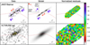 |
Fig. 3. Results from the modeling of the lensed arclet LAP1 using our forward-modeling procedure. The top-left panel shows the co-added flux of the Balmer lines (Hγ + Hβ + Hα) from the NIRSpec IFS datacube, where the blue circles indicate the position of the B1,2 mirror images and the red curve is the critical line corresponding to a source redshift z = 6.64 passing through the merged A1,2 images. The top-mid panel shows the corresponding model image; the inset shows the source plane configuration of A and B, where we also indicate the physical scale and the caustic line. The top-right panel shows the normalized residuals, (Data − Model)/σ. The bottom panels similarly show the GravityFM modeling of the VLT/MUSE Lyα image, with overlaid Lyα emission contours (in yellow) obtained from the NIRSpec datacube. |
We use the forward-modeling tool GravityFM to fit the surface brightness distribution of LAP1 obtained by co-adding the Balmer line flux within the NIRSpec IFU. This novel method – based on the Python library pyLensLib (Meneghetti 2021) and already used in Bergamini et al. (2023) – will be described in detail in a forthcoming paper by Bergamini et al. (in prep.). Briefly, by implementing a Bayesian approach and using the deflection maps from a cluster lens model, GravityFM reconstructs the structural parameter and associated errors of one or more background sources by minimizing the residuals between their extended model-predicted and observed multiple images. With GravityFM, one can add local corrections to the deflection maps of the cluster lens model. However, in our analysis, we assume the deflection field to be fixed, a decision motivated by the aforementioned high precision of the B23new macro model in reproducing the positions of all multiple images, including B1 and B2. Figure 3 shows the results of this forward model optimization. The triple-knot morphology is well reproduced with two circular components parameterized as Sérsic profiles on the source plane. The first component, named A, produces two unresolved images falling on the critical line (A1,2 in Fig. 3), while the second component, B, is responsible for the two mirrored emissions B1,2 on either side of the critical line, each of them marginally elongated along the tangential direction (we note that the telescope point spread function (PSF) at 5 μm is of the order of 1.5 spaxels; see Fig. 3). In the optimization procedure, the position, total luminosity, effective radius, and Sérsic index of both sources are free parameters, which are left free to vary with large uniform priors.
The residuals in Fig. 3, normalized by the noise measured on the image plane, show the goodness of the fit of the extended source. The bottom panel shows that the same model, optimized for the Balmer lines, also well reproduces the MUSE Lyα emission, in which the multiple single images are clearly not resolved. On the other hand, the NIRSpec Lyα emission (see overlaid yellow contours) indicates that the Lyα region is close to the central knot of LAP1. Although the detailed geometrical configuration on the source plane is still uncertain and based on emitting lines only, it is worth noting that the individual components A and B are separated by ∼150 pc on the source plane – with a formal statistical error of less than 10% – and have estimated sizes of < 5 pc and a few tens of parsecs, respectively.
Figure 4 shows the magnification map on LAP1, with the contours of the observed components A1,2 and B1,2 overlaid. The resulting best magnification factors at the median model-predicted positions of B1 and B2 are  and
and  , respectively, with relative statistical errors of ∼10%. The 68% central intervals were derived by extracting the total(tangential) magnification μtot(μtang) at the model-predicted positions over 500 realizations of the lens model, by sampling the posterior probability distribution function with a Bayesian Markov chain Monte Carlo (MCMC) technique. Such statistical errors do not include systematic errors, which likely dominate the uncertainty in this large amplification regime (e.g., Meneghetti et al. 2017). Similarly, from the same 500 magnification maps, the best magnification of LAP1 calculated within the elongated aperture (shown in Fig. 1) is μtot = 120 ± 9. This value is used when delensing the physical properties of LAP1. The corresponding median tangential stretch is also large, μtang ≃ 55 (see Table 1). The magnification of component A is formally very large, μtot(A1, 2) > 500. In the following section, we discuss the physical properties of the full arclet LAP1, and discuss its subcomponents, A and B, in Sect. 5.3.
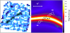 |
Fig. 4. Magnification map extracted from the B23new lens model is shown in the right panel, with contours marking the stacked, triply imaged Balmer line emission produced by the A and B components (see the left panel with the same contours). The two mirrored images B1 and B2 and A1,2 are labeled on the color-coded μtot map (adopting a square root scale). The lines corresponding to μtot = 100 are also overlaid in green. |
5. Discussion
It is worth stressing that the source-plane reconstruction is based only on the nebular emission lines, as no stellar counterpart has yet been detected. The two main emitting regions (A and B) – separated by only ∼150 pc (see source plane diagram in Fig. 3) – could either be part of a larger complex or isolated. However, regardless of its morphological structure, the magnified region shows a remarkable deficit of oxygen lines compared to the Balmer emission (e.g., [O III]λ5007/Hβ ≃ 0.55, see Table 1), implying a very low gas-phase metallicity. It is also worth emphasizing that such a result is lens-model-independent, because it is based on flux ratios and is not sensitive to possible flux-calibration issues (which appear minimal in any case; see Appendix A) given the small wavelength differences between the Balmer and metal lines.
5.1. A low-luminosity and low-mass efficient ionizing emitter
The 2σ magnitude limit of the arclet (LAP1) inferred from the stacked JWST images of 30.4 (Sect. 2) and the median magnification μtot ≃ 120 extracted from the same region (Sect. 4) correspond to a rest-frame delensed ultraviolet magnitude at 2000 Å mUV > 35.6, or an absolute MUV of fainter than −11.2. This luminosity corresponds to a stellar mass of 5 × 10³ M⊙, if we adopt a Starburst99 (Leitherer et al. 2014) instantaneous burst scenario, a Salpeter IMF, and the lowest available metallicity (1/20 Z⊙) with an age of younger than 10 Myr5. Uncertainties affect this conversion, such as the unknown underlying ultraviolet slope correction between 1500 Å and 2000 Å, the assumed IMF, metallicity, magnification, and so on. The stellar mass limit associated to LAP1 (the entire arclet) can be relaxed to 104 M⊙, a value similar to that inferred by Vanzella et al. (2020) using the HFF photometric upper limit (a subcomponent of LAP1 is discussed in Sect. 5.3). As discussed in Sect. 2, there is also no clear detection of LAP1 in the JWST bands redder than F200W, either individually or in their stacked version. In particular, it is worth noting that the measured line fluxes from Hγ, Hβ, and [O III]λλ4959, 5007 – which fall in the F356W band – correspond to a magnitude in the same band of ≃30.4, a value which is out of reach at the present depth, even assuming a point-source morphology.
The undetected stellar counterparts of LAP1 also make the equivalent width estimates of the lines unconstrained and only lower limits can be derived. In general, possible different sizes of the stellar and nebular components might be subject to different amplification values, making the equivalent widths dependent on the lens model (see discussion in Vanzella et al. 2020). However, if we assume that the stellar and nebular emissions are amplified by the same factor (both originate from the same physical region), the equivalent widths do not depend on the lens model and correspond to 3σ lower limits of 370(2020) Å rest-frame for Lyα(Hα) (see Table 1). These large values imply high ionizing photon production efficiency (ξion), metal-poor conditions (see Sect. 5.2), and ages of a few million years at most (e.g., Withers et al. 2023; Maseda et al. 2020; Raiter et al. 2010; Inoue 2011; Schaerer 2002, 2003). From the Hα and the (upper-limit) ultraviolet luminosities, we infer a 2σ lower limit estimate of the ionizing photon production efficiency of log(ξion[erg Hz−1]) > 26 (neglecting dust attenuation and assuming no escaping ionizing photons). Such a high value is reminiscent of that reported by Maseda et al. (2020) at z ∼ 4 − 5 for faint high-equivalent-width Lyα emitters with MUV ≃ −16. It is worth stressing that these limits remain relatively uncertain, as the stellar counterpart remains undetected.
5.2. LAP1, a hyper metal-poor system
A sample of extremely metal-poor galaxies (EMPGs; e.g., Annibali & Tosi 2022) in the local Universe and at moderate redshift (z ∼ 3 − 4) was recently collected by Nishigaki et al. (2023, and references therein), with additional candidates selected from JWST observations. These include EMPGs with 0.01 < Z < 0.1 Z⊙ and the authors note a deficit of hyper metal-poor cases (Z < 0.01 Z⊙), suggesting that a metallicity floor may be present at Z ∼ 0.01 Z⊙, particularly in the local Universe. The search for hyper metal-poor conditions is often carried out in the high-redshift Universe, where much lower mean metallicity of the IGM is expected: Z < 0.001 Z⊙ (e.g. Madau & Dickinson 2014). Recently, Curti et al. (2023) found a shallow slope at the low-mass end of the mass–metallicity relation at z = 3 − 10, with ≃107 M⊙ galaxies showing 12 + log(O/H)≃7.2 (see also Yang et al. 2023), where the solar value is 12 + log(O/H)⊙ = 8.69 ± 0.05 (Asplund et al. 2009). At fainter luminosities, Maseda et al. (2023) identified low-metallicity galaxies in ultra-deep MUSE observations at z = 3 − 6.7 with Z = (2 − 30)% Z⊙, preferentially showing strong Lyα emission (exceeding 120 Å rest-frame equivalent width).
We employed indirect metallicity indexes – based on the strong-line method used in the literature – for the estimation of gas metallicity (e.g., Pagel et al. 1979; Maiolino & Mannucci 2019; Nakajima et al. 2023; Katz et al. 2023; Curti et al. 2023; Maseda et al. 2023; Maiolino et al. 2008), in particular the R23 = ([O III]λλ4959, 5007 + [O II]λ3727, 3729)/Hβ and R3 = ([O III]λ5007/Hβ), along with the O32 index as a tracer of the ionization parameter (Kewley & Dopita 2002), O32 = ([O III]λλ4959, 5007/[O II]λ3727, 3729). As the calibration of such indexes typically spans the range 12 + log(O/H) > 7 (e.g., Sanders et al. 2023), in the case of LAP1, such calibrations need to be extended to slightly lower values.
As discussed by Izotov et al. (2021), a common problem of the strong-line method is the dependency on the ionization parameter, which increases the scatter of the conversion factor at low metallicity. Figure 5 shows the photoionization model predictions of the R23 and R3 indexes down to 12 + log(O/H) = 5.5 as a function of the ionization parameter, as calculated by Nakajima et al. (2022), along with the location of LAP1 described in this work. The inferred R23 =  and R3 =
  implies 6 < 12 + log(O/H) < 7, with the exact value depending on the ionization parameter. Izotov et al. (2021) introduced the O32 index in the oxygen abundance estimator in order to take into account the ionization parameter and reduce the scatter in the conversion at low metallicity, 12 + log(O/H) < 7.06.
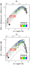 |
Fig. 5. Photoionization model predictions of the R23 (top) and R3 (bottom) indexes based on the binary evolution SEDs (BPASS). The model tracks (dashed lines) span the ionization parameter log(U) from −3.5 (thin lines) to −0.5 (thick lines) with a step of 0.5 dex. The gas density is fixed to 100 cm−3. The models encompass the scatter of data points and the dependency on the EW(Hβ) by changing the ionization parameter. The datapoints are those collected by Nakajima et al. (2022) for which accurate metallicities were measured with the direct Te method (figures adapted from Nakajima et al. 2022). |
LAP1 shows faint [O III]λ5007 and an the absence of [O II]λ3727, corresponding to a lower limit of O32 > 3(6) at 2(1)σ. In the following, we consider the total flux of the doublet [O III]λλ4959, 5007 as inferred from the observed [O III]λ5007 (which is the component with the highest S/N, of namely 4.2), fixing the ratio of the doublet to the theoretical value given by atomic physics, [O III]λ5007/[O III]λ4959 = 2.98 (Storey & Zeippen 2000, and see the notes of Table 1). Moreover, the upper limit of the flux for the unresolved doublet [O II]λ3727, 3729 (i.e., including both components) is derived by propagating the error spectrum at λ ≃ 2.8474 μm considering three slices, roughly sampling the dispersion element given by the prism mode. Adopting the above R23 value and O32 1σ limit for LAP1, Izotov et al. Eq. (5) gives 12 + log(O/H) < 6.3 (or Z < 0.004 Z⊙). This value is also consistent with those extrapolated from the photoionization models of Nakajima et al. (2022) when a high-ionization parameter is considered (high Hβ equivalent widths), as shown in Fig. 5. Figure 6 shows the location of LAP1 in the mass–metallicity plane compared to a collection of measurements performed in the local and high-redshift Universe. While the bulk of current estimates span the range of stellar masses higher than 105 M⊙ and Z > 0.01 Z⊙, with galaxies at the lower mass tail approaching the extremely metal-poor domain, LAP1 lies in the region of the hyper metal-poor systems with Z < 0.01 Z⊙, and among the lowest stellar mass star-forming regions probed in the first billion years of cosmic history, breaking the low-metallicity floor currently observed (Nishigaki et al. 2023). It is worth noting that the low stellar mass inferred for LAP1 might imply stochastic effects on its ultraviolet properties due to IMF sampling (e.g., Stanway & Eldridge 2023), such that the number of massive O-type stars (the stellar ionizers) could be penalized, resulting in an intrinsically weak [O III] emission. However, the very large ξion derived in the previous section from Balmer emissions, ξion ≳ 26, would imply a prominent [O III] equivalent width in typical metallicity conditions, 12 + log(O/H) > 7, larger than 1500 − 2000 Å rest-frame (as expected from modeling, e.g., Chevallard et al. 2018 and recently inferred with JWST, e.g., Tang et al. 2023), something which is not observed in LAP1. It is also worth noting that the same modeling of Stanway & Eldridge (2023) predict typically higher ξion as metallicity decreases, at the given stellar mass, supporting the low gas-phase metallicity interpretation for LAP1.
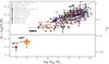 |
Fig. 6. Gas metallicity vs. stellar mass from a collection of different surveys and categories of sources in the local and high-redshift Universe (as reported in the legend; Hirschauer et al. 2022; Berg et al. 2022; Izotov et al. 2018, 2019; Nishigaki et al. 2023; Yang et al. 2017a,b; Nakajima et al. 2023; Matthee et al. 2023; Rhoads et al. 2023; Curti et al. 2023). The star-forming region described in this work – LAP1 at z = 6.639 and its subcomponent B – are marked with stars in the bottom-left corner of the figure and lie below the extremely metal-poor plateau identified to date (EMPG), approximately indicated with a horizontal shaded stripe. |
5.3. Subcomponents of LAP1, a possible pure line emitter approaching the pristine stars
So far, we have discussed the properties of the LAP1 region as it appears on the image plane. The strong-lensing forward modeling suggests that the subcomponents A and B are separated by ∼150 pc on the source plane with estimated sizes of < 5 pc and a few tens of parsecs, respectively. The comparison between the spectra extracted from components A and B and the arclet LAP1 is reported in Fig. B.2. There are two facts emerging from the NIRSpec data: (1) at positions A1,2, all the lines are detected (including weak [O III]λ5007), while (2) only the Balmer lines are currently measured at the locations B1,2. The faintness of [O III]λ5007 at B1,2 would imply an even more severe deficit of oxygen in B. In this case, the conversion to metallicity used in the previous section based on O32 cannot be used as the O32 index is not defined. Moreover, when extracting individual spectra, the overall S/N decreases, especially for the Hβ line. We therefore rely on the Hα emission from B1+B2 and adopt the ratio Hα/Hβ ≃ 2.8 (case B) to infer the metallicity. The inferred R3 < 0.2 and R23 < 0.4 (at 1σ) would correspond to 12 + log(O/H) < 6 (or Z < 0.002 Z⊙) for component B, assuming the upper envelope of the ionization parameter grid (see red arrows in Fig. 5). The Hα emissions at B1,2 are slightly elongated but still nucleated, and the magnitude limits calculated in the stacked JWST image (F115W, F150W and F200W) at those locations provide even fainter limits, of namely m2000 = 32.4 at 2σ within a circular aperture of 0.12″ diameter (corresponding to 3 × FWHM in F115W and 2 × FWHM in F200W of NIRCam imaging). The magnification for each of the mirrored images B1,2 is μtot ≃ 100, which implies an absolute magnitude M2000 fainter than −9.4 (or intrinsic m2000 > 37.4). This limit would correspond to a stellar mass of the order of (or smaller than) 103 M⊙ under the same assumptions as in the previous section. Interestingly, the above magnitude also corresponds to the expected magnitude of a single 1000 M⊙ PopIII star (Windhorst et al. 2018; Park et al. 2023) placed at z = 7. Though still speculative, component B (see the red star symbol in Fig. 6) might be the lowest metallicity portion of LAP1.
Finally, as Hα traces the same gas that produces Lyα, we would also expect Lyα emission at locations B1,2, where Hα is detected. However, there is an apparent deficit of Lyα emission at those positions, at least at the available depth. On the other hand, Lyα emission is present in the central knot, A1,2, where [O III]λ5007 and Hα are also detected (see Fig. 1). The resonant nature of the Lyα line (e.g., Dijkstra 2014) and the geometry of the emitting regions offer a possible explanation. Assuming that the IGM attenuation of Lyα is the same for A1,2 and B1,2 and that there is no dust absorption, the deficit can be ascribed to different spatial distributions of the Lyα and Hα emitting regions, with Lyα subjected to radiative transfer processes and eventually emerging from a region that is larger than the one emitting Hα (which is not resonant). This would imply that Lyα is subjected to lower magnification than Hα, preventing us from detecting it.
Another intriguing possible reason for the lack of continuum emission is that component B is undergoing Hα emission from recombination on the surface of a self-shielding system (often referred to as fluorescence) induced by the escaping ionizing radiation from component A, in which a very metal-poor stellar complex (whose stellar component is traced by faint [O III]λ5007) with MUV ≃ −10 (or fainter) acts as an efficient ionizer. Also, in this case, the Lyα emission might be attenuated by radiative transfer and magnification effects as described above. This would be the first indirect probe of escaping ionizing radiation in the reionization epoch at small spatial scales (Mas-Ribas et al. 2017a,b; Rauch et al. 2011; Runnholm et al. 2023 for a similar study in the local Universe). In addition, in this scenario, the equivalent widths of the Balmer lines at B1,2 would be formally infinite, losing their physical meaning. It is worth stressing that the still missing stellar component (from JWST imaging) and the location of A1,2 on the critical line (formally with μtot > 500) make any further detailed analysis challenging. Investigation of these possible scenarios and an in-depth study of component A (A1,2) will require higher S/N, and we aim to achieve this in future work.
6. Conclusions
We present JWST follow-up observations of an extremely faint, highly magnified Lyα arclet originally identified at z = 6.639 with HFF and VLT/MUSE deep observations, and evidence suggesting it could host extremely metal-poor stars (Vanzella et al. 2020). JWST spectroscopic data reveal new, key information on the nature of this source, corroborating evidence that it is the most metal-poor star-forming complex currently known, observed at an epoch of 800 Myr after the Big Bang. Our results can be summarized as follows:
(1) JWST/NIRSpec IFU observations confirm the redshift of the underlying forming system, z = 6.639, by means of hydrogen Balmer lines, Hγ, Hβ, and Hα, with a remarkably faint oxygen line, [O III]λλ4959, 5007 – the only metal line detected – with a ratio [O III]λ5007/Hβ = 0.55 ± 0.15. The flux ratios of the Balmer lines are consistent (within 2σ) with case B recombination theory, suggesting negligible dust extinction. The same case B and the ratio Hα/Lyα ≃ 5 imply that part of the Lyα line is attenuated by circumgalactic or intergalactic neutral gas or is escaping on larger scales.
(2) No significant stellar counterpart is detected in the stacked JWST/NIRCam, NIRISS, and Hubble images down to a UV magnitude m2000 ≃ 30.4 at 2σ level, corresponding to an intrinsic magnitude m2000 > 35.8 (or fainter than M2000 = −11). Such low luminosity implies a stellar mass of ≲104 M⊙, assuming no dust extinction and an instantaneous burst scenario. This is currently the faintest confirmed star-forming complex found in the reionization era.
(3) The deficiency of metal lines of LAP1 implies an extremely low metallicity, 12 + log(O/H) < 6.3 (Z < 0.004 Z⊙). With such a low metallicity and the above upper limit on the stellar mass, LAP1 breaks the metallicity floor (Z ≳ 0.01 Z⊙) observed in a variety of systems in the local and distant Universe, thus entering the hyper metal-poor regime (Z < 0.01 Z⊙) and approaching the properties expected for a pristine star-forming region. A possible detection of He IIλ1640 emission remains tentative and will require further exploration.
(4) Based on a high-precision strong lensing model of MACS J0416, the highly elongated nebular-line morphology of LAP1, straddling the critical line at z = 6.64, can be reproduced with two components, A and B, spanning ∼300 pc on the source plane. LAP1-B is fainter than MUV = −10, with undetected metal lines, likely lying at the lowest stellar mass and metallicity of the mass-metallicity relation (Fig. 6). LAP1-A is subject to extreme magnification (μ ≫ 100), falling on the critical line, appears rather compact, and shows faint [O III] emission. The nature of LAP1-A is still uncertain and will be studied in future work. The possibility that the Balmer emission in B is induced by escaping ionizing radiation coming from component A is also an option, and, in such a case, is the first indirect probe of a transverse escaping ionizing radiation during reionization.
Overall, LAP1 (A+B) represents an intriguing remote region of forming stars, possibly approaching the long-sought pristine zero-metal conditions. Further JWST observations and future facilities, such as the ELT, will be crucial for probing key spectral lines such as He IIλ1640 of Population-III regions, reaching even fainter flux limits than those that JWST or 8−10 m class telescopes can achieve now.
Finally, it is worth emphasizing that LAP1 was a serendipitous discovery by means of blind IFU spectroscopy obtained with VLT/MUSE through the Lyα detection, as a pure line emitter. The results presented in this work were only achievable thanks to the IFU JWST/NIRSpec spectroscopy, which allowed us to perform a blind two-dimensional characterization of the emission lines along the arclet and the regions across the critical line. Therefore, integral filed spectroscopy plays a crucial role in this kind of investigation.
For example, in the fiducial model of Vikaeus et al. (2022), a 104 M⊙ system younger than 10 Myr would have a He IIλ1640 line flux of 4.5 × 10⁻²² erg s−1 cm−2 at z = 10.
At the time of writing, this step can introduce a systematic uncertainty as high as 10% due to a simplification in the reference files (Böker et al. 2023).
The inferred redshift appears slightly higher than the value obtained from VLT/MUSE, z = 6.629. This discrepancy is not fully clear at the time of writing. However, we note that the JWST/NIRSpec wavelength calibration is still under verification especially in the case of the IFS mode (see Sect. 6.3 in Böker et al. 2023). This possible shift does not affect the conclusions of this work.
It is worth noting that the NIRSpec spaxel angular scale of 0.1″ undersamples the JWST PSF at λ < 2.5 μm.
This value was inferred after rescaling the Starburst99 reference case of a 106 M⊙ system (which produces a peak 1500 Å luminosity of L1500 ≃ 1039.5 erg s−1 Å−1) to the L1500 < 1037.2 erg s−1 Å−1 of LAP1. The dust extinction is neglected here and the magnitude correction dm from 2000 Å to 1500 Å –depending on the ultraviolet slope β (Fλ ∼ λβ)– is not significant; dm < +0.3 if the slope is shallower than β = −3.
Equation (5) of Izotov et al. (2021): 12 + log10(O/H) = 0.958 × log10(R23 − (0.080 − 0.00078 × O32) × O32) + 6.805.
Acknowledgments
We thank the anonymous referee for the careful reading and constructive comments. We thank Raffaella Schneider for useful comments. We thank K. Nakajima who provided us part of the information used in Fig. 5 and the extended calibrations of the indexes R23 and R3 down to 12 + log(O/H) = 5.5. This work is based on observations made with the NASA/ESA/CSA James Webb Space Telescope (JWST) and Hubble Space Telescope (HST). These observations are associated with JWST GO program n.1908 (PI: E. Vanzella) and GTO n.1208 (CANUCS, PI: C. Willot). We acknowledge financial support through grants PRIN-MIUR 2017WSCC32 and 2020SKSTHZ. M.M. acknowledges support from INAF Minigrant “The Big-Data era of cluster lensing”. M.C. acknowledges support from INAF Mini-grant “Reionization and Fundamental Cosmology with High-Redshift Galaxies”. E.V. acknowledges support from the INAF GO Grant 2022 “The revolution is around the corner: JWST will probe globular cluster precursors and Population III stellar clusters at cosmic dawn”. M.B. and G.R. acknowledge support from the Slovenian national research agency ARRS through grant N1-0238. K.I.C. acknowledges funding from the Netherlands Research School for Astronomy (NOVA) and the Dutch Research Council (NWO) through the award of the Vici Grant VI.C.212.036. M.G. thanks the Max Planck Society for support through the Max Planck Research Group. This research has made use of NASA’s Astrophysics Data System, QFitsView, and SAOImageDS9, developed by Smithsonian Astrophysical Observatory. Additionally, this work made use of the following open-source packages for Python and we are thankful to the developers of these: Matplotlib (Hunter 2007), MPDAF (Piqueras et al. 2019), PyMUSE (Pessa et al. 2020), Numpy (van der Walt et al. 2011). We would like to express our deepest gratitude to our colleague and friend Mario Nonino for inspiring discussions over the years on all aspects related to the quest for the first generation of stars in the Universe, and particularly for sharing with us his profound knowledge on data analysis and reduction; Mario, unfortunately, passed away at the age of 63, during the acceptance of this work.
References
- Abel, T., Bryan, G. L., & Norman, M. L. 2002, Science, 295, 93 [CrossRef] [Google Scholar]
- Annibali, F., & Tosi, M. 2022, Nat. Astron., 6, 48 [NASA ADS] [CrossRef] [Google Scholar]
- Asplund, M., Grevesse, N., Sauval, A. J., & Scott, P. 2009, ARA&A, 47, 481 [NASA ADS] [CrossRef] [Google Scholar]
- Berg, D. A., James, B. L., King, T., et al. 2022, ApJS, 261, 31 [NASA ADS] [CrossRef] [Google Scholar]
- Bergamini, P., Grillo, C., Rosati, P., et al. 2023, A&A, 674, A79 [NASA ADS] [CrossRef] [EDP Sciences] [Google Scholar]
- Bik, A., Östlin, G., Menacho, V., et al. 2018, A&A, 619, A131 [NASA ADS] [CrossRef] [EDP Sciences] [Google Scholar]
- Böker, T., Beck, T. L., Birkmann, S. M., et al. 2023, PASP, 135, 1045 [Google Scholar]
- Boyett, K. N. K., Stark, D. P., Bunker, A. J., Tang, M., & Maseda, M. V. 2022, MNRAS, 513, 4451 [NASA ADS] [CrossRef] [Google Scholar]
- Brammer, G., Strait, V., Matharu, J., & Momcheva, I. 2022, https://zenodo.org/record/6672538 [Google Scholar]
- Bromm, V. 2013, Rep. Progr. Phys., 76, 112901 [CrossRef] [Google Scholar]
- Bromm, V., Coppi, P. S., & Larson, R. B. 2002, ApJ, 564, 23 [Google Scholar]
- Calura, F., Vanzella, E., Carniani, S., et al. 2021, MNRAS, 500, 3083 [Google Scholar]
- Cameron, A. J., Saxena, A., Bunker, A. J., et al. 2023, A&A, 677, A115 [NASA ADS] [CrossRef] [EDP Sciences] [Google Scholar]
- Castellano, M., Pentericci, L., Fontana, A., et al. 2017, ApJ, 839, 73 [NASA ADS] [CrossRef] [Google Scholar]
- Chevallard, J., Charlot, S., Senchyna, P., et al. 2018, MNRAS, 479, 3264 [Google Scholar]
- Cresci, G., Tozzi, G., Perna, M., et al. 2023, A&A, 672, A128 [NASA ADS] [CrossRef] [EDP Sciences] [Google Scholar]
- Curti, M., Maiolino, R., Carniani, S., et al. 2023, A&A, submitted [arXiv:2304.08516] [Google Scholar]
- De Barros, S., Oesch, P. A., Labbé, I., et al. 2019, MNRAS, 489, 2355 [NASA ADS] [CrossRef] [Google Scholar]
- Dijkstra, M. 2014, PASA, 31, e040 [Google Scholar]
- Endsley, R., Stark, D. P., Chevallard, J., & Charlot, S. 2021, MNRAS, 500, 5229 [Google Scholar]
- Ferruit, P., Jakobsen, P., Giardino, G., et al. 2022, A&A, 661, A81 [NASA ADS] [CrossRef] [EDP Sciences] [Google Scholar]
- Gardner, J. P., Mather, J. C., Abbott, R., et al. 2023, PASP, 135, 1048 [Google Scholar]
- Hartwig, T., Yoshida, N., Magg, M., et al. 2018, MNRAS, 478, 1795 [CrossRef] [Google Scholar]
- Hirano, S., Hosokawa, T., Yoshida, N., et al. 2014, ApJ, 781, 60 [NASA ADS] [CrossRef] [Google Scholar]
- Hirschauer, A. S., Salzer, J. J., Haurberg, N., Gronwall, C., & Janowiecki, S. 2022, ApJ, 925, 131 [NASA ADS] [CrossRef] [Google Scholar]
- Hunter, J. D. 2007, Comput. Sci. Eng., 9, 90 [NASA ADS] [CrossRef] [Google Scholar]
- Inoue, A. K. 2011, MNRAS, 415, 2920 [NASA ADS] [CrossRef] [Google Scholar]
- Izotov, Y. I., Thuan, T. X., Guseva, N. G., & Liss, S. E. 2018, MNRAS, 473, 1956 [NASA ADS] [CrossRef] [Google Scholar]
- Izotov, Y. I., Guseva, N. G., Fricke, K. J., & Henkel, C. 2019, A&A, 623, A40 [NASA ADS] [CrossRef] [EDP Sciences] [Google Scholar]
- Izotov, Y. I., Thuan, T. X., & Guseva, N. G. 2021, MNRAS, 504, 3996 [NASA ADS] [CrossRef] [Google Scholar]
- Jakobsen, P., Ferruit, P., Alves de Oliveira, C., et al. 2022, A&A, 661, A80 [NASA ADS] [CrossRef] [EDP Sciences] [Google Scholar]
- Katz, H., Kimm, T., Ellis, R. S., Devriendt, J., & Slyz, A. 2023, MNRAS, 524, 351 [CrossRef] [Google Scholar]
- Kehrig, C., Vílchez, J. M., Guerrero, M. A., et al. 2018, MNRAS, 480, 1081 [NASA ADS] [Google Scholar]
- Kewley, L. J., & Dopita, M. A. 2002, ApJS, 142, 35 [Google Scholar]
- Klessen, R. S., & Glover, S. C. O. 2023, ARA&A, 61, 65 [NASA ADS] [CrossRef] [Google Scholar]
- Leitherer, C., Ekström, S., Meynet, G., et al. 2014, ApJS, 212, 14 [Google Scholar]
- Liu, B., & Bromm, V. 2020, MNRAS, 497, 2839 [NASA ADS] [CrossRef] [Google Scholar]
- Lotz, J. M., Koekemoer, A., Coe, D., et al. 2017, ApJ, 837, 97 [Google Scholar]
- Madau, P., & Dickinson, M. 2014, ARA&A, 52, 415 [Google Scholar]
- Maio, U., Ciardi, B., Dolag, K., Tornatore, L., & Khochfar, S. 2010, MNRAS, 407, 1003 [CrossRef] [Google Scholar]
- Maio, U., Petkova, M., De Lucia, G., & Borgani, S. 2016, MNRAS, 460, 3733 [NASA ADS] [CrossRef] [Google Scholar]
- Maiolino, R., & Mannucci, F. 2019, A&ARv, 27, 3 [Google Scholar]
- Maiolino, R., Nagao, T., Grazian, A., et al. 2008, A&A, 488, 463 [NASA ADS] [CrossRef] [EDP Sciences] [Google Scholar]
- Marshall, M. A., Perna, M., Willott, C. J., et al. 2023, A&A, in press [arXiv:2302.04795] [Google Scholar]
- Mas-Ribas, L., Dijkstra, M., & Forero-Romero, J. E. 2016, ApJ, 833, 65 [NASA ADS] [Google Scholar]
- Mas-Ribas, L., Dijkstra, M., Hennawi, J. F., et al. 2017a, ApJ, 841, 19 [Google Scholar]
- Mas-Ribas, L., Hennawi, J. F., Dijkstra, M., et al. 2017b, ApJ, 846, 11 [NASA ADS] [CrossRef] [Google Scholar]
- Maseda, M. V., Bacon, R., Lam, D., et al. 2020, MNRAS, 493, 5120 [Google Scholar]
- Maseda, M. V., Lewis, Z., Matthee, J., et al. 2023, ApJ, accepted [arXiv:2304.08511] [Google Scholar]
- Matthee, J., Mackenzie, R., Simcoe, R. A., et al. 2023, ApJ, 950, 67 [NASA ADS] [CrossRef] [Google Scholar]
- Meneghetti, M. 2021, Introduction to Gravitational Lensing: With Python Examples (Cham: Springer International Publishing) [CrossRef] [Google Scholar]
- Meneghetti, M., Natarajan, P., Coe, D., et al. 2017, MNRAS, 472, 3177 [Google Scholar]
- Merlin, E., Pilo, S., Fontana, A., et al. 2019, A&A, 622, A169 [NASA ADS] [CrossRef] [EDP Sciences] [Google Scholar]
- Nakajima, K., & Maiolino, R. 2022, MNRAS, 513, 5134 [NASA ADS] [CrossRef] [Google Scholar]
- Nakajima, K., Ouchi, M., Xu, Y., et al. 2022, ApJS, 262, 3 [CrossRef] [Google Scholar]
- Nakajima, K., Ouchi, M., Isobe, Y., et al. 2023, ApJS, accepted [arXiv:2301.12825] [Google Scholar]
- Nishigaki, M., Ouchi, M., Nakajima, K., et al. 2023, ApJ, 952, 11 [NASA ADS] [CrossRef] [Google Scholar]
- Oke, J. B., & Gunn, J. E. 1983, ApJ, 266, 713 [NASA ADS] [CrossRef] [Google Scholar]
- Osterbrock, D. E. 1989, Astrophysics of Gaseous Nebulae and Active Galactic Nuclei (Mill Valley: University Science Books) [Google Scholar]
- Pagel, B. E. J., Edmunds, M. G., Blackwell, D. E., Chun, M. S., & Smith, G. 1979, MNRAS, 189, 95 [NASA ADS] [CrossRef] [Google Scholar]
- Pallottini, A., Ferrara, A., Gallerani, S., Salvadori, S., & D’Odorico, V. 2014, MNRAS, 440, 2498 [NASA ADS] [CrossRef] [Google Scholar]
- Park, J., Ricotti, M., & Sugimura, K. 2021, MNRAS, 508, 6176 [NASA ADS] [CrossRef] [Google Scholar]
- Park, J., Ricotti, M., & Sugimura, K. 2023, MNRAS, 521, 5334 [NASA ADS] [CrossRef] [Google Scholar]
- Perna, M., Arribas, S., Marshall, M., et al. 2023, A&A, in press [arXiv:2304.06756] [Google Scholar]
- Pessa, I., Tejos, N., & Moya, C. 2020, ASP Conf. Ser., 522, 61 [Google Scholar]
- Piqueras, L., Conseil, S., Shepherd, M., et al. 2019, ASP Conf. Ser., 521, 545 [Google Scholar]
- Raiter, A., Schaerer, D., & Fosbury, R. A. E. 2010, A&A, 523, A64 [NASA ADS] [CrossRef] [EDP Sciences] [Google Scholar]
- Rauch, M., Becker, G. D., Haehnelt, M. G., et al. 2011, MNRAS, 418, 1115 [NASA ADS] [CrossRef] [Google Scholar]
- Rhoads, J. E., Wold, I. G. B., Harish, S., et al. 2023, ApJ, 942, L14 [NASA ADS] [CrossRef] [Google Scholar]
- Rigby, J., Perrin, M., McElwain, M., et al. 2023, PASP, 135, 048001 [NASA ADS] [CrossRef] [Google Scholar]
- Rinaldi, P., Caputi, K. I., Costantin, L., et al. 2023, ApJ, 952, 143 [NASA ADS] [CrossRef] [Google Scholar]
- Runnholm, A., Hayes, M. J., Lin, Y. H., et al. 2023, MNRAS, 522, 4275 [NASA ADS] [CrossRef] [Google Scholar]
- Rydberg, C.-E., Zackrisson, E., Lundqvist, P., & Scott, P. 2013, MNRAS, 429, 3658 [NASA ADS] [CrossRef] [Google Scholar]
- Salvadori, S., Schneider, R., & Ferrara, A. 2007, MNRAS, 381, 647 [NASA ADS] [CrossRef] [Google Scholar]
- Sanders, R. L., Shapley, A. E., Topping, M. W., Reddy, N. A., & Brammer, G. B. 2023, ApJ, submitted [arXiv:2303.08149] [Google Scholar]
- Sarmento, R., Scannapieco, E., & Cohen, S. 2018, ApJ, 854, 75 [NASA ADS] [CrossRef] [Google Scholar]
- Sarmento, R., Scannapieco, E., & Côté, B. 2019, ApJ, 871, 206 [CrossRef] [Google Scholar]
- Schaerer, D. 2002, A&A, 382, 28 [NASA ADS] [CrossRef] [EDP Sciences] [Google Scholar]
- Schaerer, D. 2003, A&A, 397, 527 [NASA ADS] [CrossRef] [EDP Sciences] [Google Scholar]
- Schaerer, D., Fragos, T., & Izotov, Y. I. 2019, A&A, 622, L10 [NASA ADS] [CrossRef] [EDP Sciences] [Google Scholar]
- Senchyna, P., Stark, D. P., Mirocha, J., et al. 2020, MNRAS, 494, 941 [CrossRef] [Google Scholar]
- Senchyna, P., Stark, D. P., Charlot, S., et al. 2021, MNRAS, 503, 6112 [NASA ADS] [CrossRef] [Google Scholar]
- Shibuya, T., Ouchi, M., Harikane, Y., et al. 2018, PASJ, 70, S15 [Google Scholar]
- Shirazi, M., & Brinchmann, J. 2012, MNRAS, 421, 1043 [NASA ADS] [CrossRef] [Google Scholar]
- Sobral, D., Matthee, J., Brammer, G., et al. 2019, MNRAS, 482, 2422 [Google Scholar]
- Stanway, E. R., & Eldridge, J. J. 2023, MNRAS, 522, 4430 [NASA ADS] [CrossRef] [Google Scholar]
- Storey, P. J., & Zeippen, C. J. 2000, MNRAS, 312, 813 [NASA ADS] [CrossRef] [Google Scholar]
- Tang, M., Stark, D. P., Chen, Z., et al. 2023, MNRAS, 526, 1657 [NASA ADS] [CrossRef] [Google Scholar]
- Tornatore, L., Ferrara, A., & Schneider, R. 2007, MNRAS, 382, 945 [NASA ADS] [CrossRef] [Google Scholar]
- Trussler, J. A. A., Conselice, C. J., Adams, N. J., et al. 2023, MNRAS, 525, 5328 [NASA ADS] [CrossRef] [Google Scholar]
- Übler, H., Maiolino, R., Curtis-Lake, E., et al. 2023, A&A, 677, A145 [NASA ADS] [CrossRef] [EDP Sciences] [Google Scholar]
- van der Walt, S., Colbert, S. C., & Varoquaux, G. 2011, Comput. Sci. Eng., 13, 22 [Google Scholar]
- Vanni, I., Salvadori, S., & Skúladóttir, Á. 2023, MemSAIt, accepted [arXiv:2305.02358] [Google Scholar]
- Vanzella, E., Calura, F., Meneghetti, M., et al. 2017, MNRAS, 467, 4304 [Google Scholar]
- Vanzella, E., Calura, F., Meneghetti, M., et al. 2019, MNRAS, 483, 3618 [Google Scholar]
- Vanzella, E., Meneghetti, M., Caminha, G. B., et al. 2020, MNRAS, 494, L81 [Google Scholar]
- Vanzella, E., Caminha, G. B., Rosati, P., et al. 2021, A&A, 646, A57 [EDP Sciences] [Google Scholar]
- Venditti, A., Graziani, L., Schneider, R., et al. 2023, MNRAS, 522, 3809 [NASA ADS] [CrossRef] [Google Scholar]
- Vikaeus, A., Zackrisson, E., & Binggeli, C. 2020, MNRAS, 492, 1706 [CrossRef] [Google Scholar]
- Vikaeus, A., Zackrisson, E., Schaerer, D., et al. 2022, MNRAS, 512, 3030 [NASA ADS] [CrossRef] [Google Scholar]
- Wang, X., Cheng, C., Ge, J., et al. 2022, ArXiv e-prints [arXiv:2212.04476] [Google Scholar]
- Williams, C. C., Tacchella, S., Maseda, M. V., et al. 2023, AAS, submitted [arXiv:2301.09780] [Google Scholar]
- Willott, C. J., Doyon, R., Albert, L., et al. 2022, PASP, 134, 025002 [CrossRef] [Google Scholar]
- Windhorst, R. A., Timmes, F. X., Wyithe, J. S. B., et al. 2018, ApJS, 234, 41 [NASA ADS] [CrossRef] [Google Scholar]
- Withers, S., Muzzin, A., Ravindranath, S., et al. 2023, ApJL, submitted [arXiv:2304.11181] [Google Scholar]
- Yajima, H., Abe, M., Fukushima, H., et al. 2023, MNRAS, 525, 4832 [NASA ADS] [CrossRef] [Google Scholar]
- Yang, H., Malhotra, S., Rhoads, J. E., & Wang, J. 2017a, ApJ, 847, 38 [NASA ADS] [CrossRef] [Google Scholar]
- Yang, H., Malhotra, S., Gronke, M., et al. 2017b, ApJ, 844, 171 [NASA ADS] [CrossRef] [Google Scholar]
- Yang, S., Lidz, A., Smith, A., Benson, A., & Li, H. 2023, MNRAS, 525, 5989 [NASA ADS] [CrossRef] [Google Scholar]
- Zackrisson, E., Rydberg, C.-E., Schaerer, D., Östlin, G., & Tuli, M. 2011, ApJ, 740, 13 [NASA ADS] [CrossRef] [Google Scholar]
- Zackrisson, E., González, J., Eriksson, S., et al. 2015, MNRAS, 449, 3057 [NASA ADS] [CrossRef] [Google Scholar]
Appendix A: Post-processing and flux calibration
We decided to perform the background subtraction directly from the reduced datacube rather than applying the specific procedure provided by the NIRSpec reduction pipeline. A limited number of sources fall in the cube field of view, meaning that a large sky region can be used to estimate the background robustly. Specifically, the background in the datacube was derived by calculating a moving median in each XY (sky coordinates) plane, with a box of 7 × 7 spaxels, corresponding to 0.7″ × 0.7″, or ≃1/20 of the field of view (3″ × 3″). The same procedure was performed by varying the window size from 3 × 3 to 11 × 11 spaxels. The few sources present in the field were masked following the NIRSpec median collapsed image and the NIRCam deep stacking, which identify the same set of sources (see Figure 1 and A.1). We found that median filter boxes ranging from 5 × 5 to 9 × 9 spaxels provide the best results, with 7 × 7 providing the best compromise.
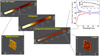 |
Fig. A.1. Scheme of the post-processing of the datacube. From top left to lower right, the reduced cube flux-calibrated in Fλ as described in Sect. 3.1, not background subtracted. Each XY plane consists of 48 by 43 spaxels (0.1″/spaxel), while 940 slices span the range 0.6 − 5.3 μm along the wavelength direction, with 1 slice sampling 50 Å. In the middle panel, the background is derived from the top left with a moving median calculated on each XY plane and removal of the outliers (see text). The bottom panel shows the background-subtracted and clipped datacube. An example of the masked sources and edges of the cube is shown in the bottom left, while the bottom right shows an extracted slice at the peak of the Hα line. In the top-right inset, the residual values per slice and the depth of the cube are reported (see details in the text). |
After subtracting the background cube from the original one, a cleaning procedure was applied on each XY plane by setting to zero the spaxel values deviating more than a given percentile threshold (percup and perclow). For the arclet, we adopt percup = 98% and perclow 2% after verifying that such a cut does not affect the extracted signal from LAP1. This clipping procedure removes single spaxels and not structures. Figure A.1 shows the median, 16%, and 84% percentiles calculated on each slice from 0.6 to 5.3 μm. The median is overall consistent with zero, and the lower and upper percentiles are symmetric.
Finally, the spectrum is extracted by summing up the corresponding spaxel values within the adopted aperture. The noise is estimated by randomly placing apertures (both of Source 1 or the arclet) within the field of view, avoiding the positions of the targets. In the case of the arclet, this translates into avoiding random positions along the diagonal direction of the datacube. For example, in the case of Source 1 at z = 2.41, 62 spectra were extracted from as many random positions (shown in green in Figure A.2). The standard and absolute median deviations provide the 1σ uncertainty of the extracted spectrum. The same procedure was performed for LAP1.
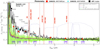 |
Fig. A.2. One-dimensional spectrum of Source 1 at z = 2.41 extracted from the aperture shown in Figure 1. The same aperture was used to compute the JWST/NIRcam, NIRISS, and Hubble photometry, all superimposed on this figure without applying any scaling factor. At the bottom, the filter names are indicated with the magnitudes of Source 1. The blue dashed lines show the filter throughputs. The green region shows the noise obtained from 62 spectra extracted with the same aperture size, placed randomly in the field of view. The blue and red lines show the absolute and standard deviation from the green envelope. |
The high S/N of Source 1 in the JWST/NIRCam and NIRISS observations also provides an additional reference for flux calibration. We extracted the spectrum from the same region as the photometric aperture (see the red ellipse in Figure 1). Photometry was performed with the A-PHOT tool (Merlin et al. 2019) on JWST and HST data. Figure A.2 shows the consistency between the photometric points and the spectrum of Source 1 without applying any correction factor. The flux calibration provided by the JWST/NIRspec pipeline appears accurate at a few percent level (Böker et al. 2023), though systematic effects may still be present on the overall normalization. We assume they are not larger than 20%, as the good agreement between photometry and spectroscopy suggests. It is worth noting that this is not affecting the inferred flux ratios reported in Table 1, especially the ratios between close (in wavelength) atomic lines.
The depth of the cleaned and flux-calibrated datacube is entirely consistent with expectations given the integration time (Figure A.1, top-right), corresponding to a magnitude of ≃30.6 per slice at 1σ at λ = 1.2 μm and within an aperture of 0.2″ × 0.2″ (4 spaxels).
Appendix B: Emission lines from LAP1
The Lyα, [O III]λ5007, and the Balmer lines Hγ, Hβ, and Hα are detected with S/N spanning the range 4 − 13 and are shown in Figure B.1, after averaging them along four slices (each slice corresponds to Δλ = 50 Å). As expected from the lens model, two multiple images of both sides of the critical line emerge in the stacked image of Balmer lines (indicated with black circles). The Lyα emission appears mainly located in the center, on top of the critical line, while [O III]λ5007 shows a smaller extension than the Balmer lines.
 |
Fig. B.1. Two-dimensional images of the most relevant lines detected at the redshift of the arclet. From left to right, the Lyα, [O III]λ5007, Hα and the sum of the Balmer lines, Hγ, Hβ, and Hα. The first and second rows show the same images, derived after averaging three slices at the wavelength position of the lines. In the second row, the knots are labeled: the black circles highlight the components B1,2 and the ellipse marks the position of source 1. The black curve outlines the critical line of the customized lens model. |
Figure B.2 shows the comparison between the one-dimensional spectra extracted individually from components A1,2, B1,2, and LAP1.
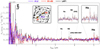 |
Fig. B.2. One-dimensional spectra extracted from individual components. The main arclet spectrum of LAP1 is shown in black, while the A1,2 and B1,2 in blue and red, respectively (as indicated in the title). The apertures from which the spectra of A1,2 and B1,2 were extracted are shown in the top-left inset in which the spaxels used are superimposed to the stacked image of Balmer lines (the same as shown in Figure B.1). The top-right insets show the zoomed regions, indicated with gray-dashed lines. |
All Tables
All Figures
|
Fig. 1. Photometric and spectroscopic observations of LAP1. Hubble Frontier Fields (Lotz et al. 2017) and JWST NIRISS NIRCam imaging from the CANUCS GTO program (Willott et al. 2022). From top left to bottom right: (1) the combined HST F435W and F606W image probing λ < 915 Å at z = 6.639. The black arrow indicates the presence of a foreground object, which is nevertheless not significantly contaminating the extracted spectrum of LAP1; (2) the 11 stacked bands from JWST/NIRCam and NIRISS, as labeled in the bottom left (white and cyan labeled filters indicate NIRCam and NIRISS, respectively); (3) the median collapse of the entire NIRSpec datacube spanning the range 0.7 − 5.2 μm (black circles indicate sources visible in the JWST and HST imaging); (4) the color composite image with the three channels blue, green, and red as indicated in the legend on the left (we note that the red channel shows the 6 stacked bands F115W, F150W, and F200W combined from NIRISS and NIRCam). The white square marks the NIRSpec FoV. The yellow circles mark the same objects as in panel 3 and the green contour outlines the 3σ Lyα from VLT/MUSE; (5)–(7) show the Lyα, [O III]λ5007, and the sum Hγ + Hβ + Hα, with the critical line (in black) and the positions of the two B1,2 components (marked with red circles), respectively; (8) shows the masks used to extract the spectra from the sources described in the text. The elongated red contour of 2.3″ × 0.2″ outlines the aperture used to extract the spectrum of the arclet (LAP1), defined on the combined image of the Balmer lines (see Appendix B), while the ellipse indicates the aperture used to extract the spectrum shown in Fig. A.2 and the magnitudes of Source 1 (z = 2.41; see Appendix A). All panels have the same scale, indicated in panel 8. The angular size of the single spaxel and the PSF at 5 μm are reported in the bottom-right inset of panel 8. |
| In the text | |
|
Fig. 2. One-dimensional NIRSpec spectrum of LAP1 (black line) extracted from the elongated aperture (“Arclet”) shown in panel 8 of Fig. 1. The most relevant lines, detected with S/N > 4, are indicated in bold red text and dashed lines. Additional undetected atomic transitions are shown with gray dotted lines at the redshift inferred from the Balmer lines, along with the uncertain He IIλ1640 detection marked in black. The green area shows the distribution of 42 spectra randomly extracted with the same aperture within the FoV. The blue and red lines show the corresponding absolute median and standard deviations, respectively. The redshift, adopted clipping threshold, and background window size used in the post-processing are given (top-right corner; see Appendix A for more details). The standard and mean absolute deviations are shown in red and blue, respectively. JWST photometric bands are outlined with blue dotted lines and are labeled at the bottom of the figure. |
| In the text | |
|
Fig. 3. Results from the modeling of the lensed arclet LAP1 using our forward-modeling procedure. The top-left panel shows the co-added flux of the Balmer lines (Hγ + Hβ + Hα) from the NIRSpec IFS datacube, where the blue circles indicate the position of the B1,2 mirror images and the red curve is the critical line corresponding to a source redshift z = 6.64 passing through the merged A1,2 images. The top-mid panel shows the corresponding model image; the inset shows the source plane configuration of A and B, where we also indicate the physical scale and the caustic line. The top-right panel shows the normalized residuals, (Data − Model)/σ. The bottom panels similarly show the GravityFM modeling of the VLT/MUSE Lyα image, with overlaid Lyα emission contours (in yellow) obtained from the NIRSpec datacube. |
| In the text | |
|
Fig. 4. Magnification map extracted from the B23new lens model is shown in the right panel, with contours marking the stacked, triply imaged Balmer line emission produced by the A and B components (see the left panel with the same contours). The two mirrored images B1 and B2 and A1,2 are labeled on the color-coded μtot map (adopting a square root scale). The lines corresponding to μtot = 100 are also overlaid in green. |
| In the text | |
|
Fig. 5. Photoionization model predictions of the R23 (top) and R3 (bottom) indexes based on the binary evolution SEDs (BPASS). The model tracks (dashed lines) span the ionization parameter log(U) from −3.5 (thin lines) to −0.5 (thick lines) with a step of 0.5 dex. The gas density is fixed to 100 cm−3. The models encompass the scatter of data points and the dependency on the EW(Hβ) by changing the ionization parameter. The datapoints are those collected by Nakajima et al. (2022) for which accurate metallicities were measured with the direct Te method (figures adapted from Nakajima et al. 2022). |
| In the text | |
|
Fig. 6. Gas metallicity vs. stellar mass from a collection of different surveys and categories of sources in the local and high-redshift Universe (as reported in the legend; Hirschauer et al. 2022; Berg et al. 2022; Izotov et al. 2018, 2019; Nishigaki et al. 2023; Yang et al. 2017a,b; Nakajima et al. 2023; Matthee et al. 2023; Rhoads et al. 2023; Curti et al. 2023). The star-forming region described in this work – LAP1 at z = 6.639 and its subcomponent B – are marked with stars in the bottom-left corner of the figure and lie below the extremely metal-poor plateau identified to date (EMPG), approximately indicated with a horizontal shaded stripe. |
| In the text | |
|
Fig. A.1. Scheme of the post-processing of the datacube. From top left to lower right, the reduced cube flux-calibrated in Fλ as described in Sect. 3.1, not background subtracted. Each XY plane consists of 48 by 43 spaxels (0.1″/spaxel), while 940 slices span the range 0.6 − 5.3 μm along the wavelength direction, with 1 slice sampling 50 Å. In the middle panel, the background is derived from the top left with a moving median calculated on each XY plane and removal of the outliers (see text). The bottom panel shows the background-subtracted and clipped datacube. An example of the masked sources and edges of the cube is shown in the bottom left, while the bottom right shows an extracted slice at the peak of the Hα line. In the top-right inset, the residual values per slice and the depth of the cube are reported (see details in the text). |
| In the text | |
|
Fig. A.2. One-dimensional spectrum of Source 1 at z = 2.41 extracted from the aperture shown in Figure 1. The same aperture was used to compute the JWST/NIRcam, NIRISS, and Hubble photometry, all superimposed on this figure without applying any scaling factor. At the bottom, the filter names are indicated with the magnitudes of Source 1. The blue dashed lines show the filter throughputs. The green region shows the noise obtained from 62 spectra extracted with the same aperture size, placed randomly in the field of view. The blue and red lines show the absolute and standard deviation from the green envelope. |
| In the text | |
|
Fig. B.1. Two-dimensional images of the most relevant lines detected at the redshift of the arclet. From left to right, the Lyα, [O III]λ5007, Hα and the sum of the Balmer lines, Hγ, Hβ, and Hα. The first and second rows show the same images, derived after averaging three slices at the wavelength position of the lines. In the second row, the knots are labeled: the black circles highlight the components B1,2 and the ellipse marks the position of source 1. The black curve outlines the critical line of the customized lens model. |
| In the text | |
|
Fig. B.2. One-dimensional spectra extracted from individual components. The main arclet spectrum of LAP1 is shown in black, while the A1,2 and B1,2 in blue and red, respectively (as indicated in the title). The apertures from which the spectra of A1,2 and B1,2 were extracted are shown in the top-left inset in which the spaxels used are superimposed to the stacked image of Balmer lines (the same as shown in Figure B.1). The top-right insets show the zoomed regions, indicated with gray-dashed lines. |
| In the text | |
Current usage metrics show cumulative count of Article Views (full-text article views including HTML views, PDF and ePub downloads, according to the available data) and Abstracts Views on Vision4Press platform.
Data correspond to usage on the plateform after 2015. The current usage metrics is available 48-96 hours after online publication and is updated daily on week days.
Initial download of the metrics may take a while.