| Issue |
A&A
Volume 677, September 2023
|
|
|---|---|---|
| Article Number | A52 | |
| Number of page(s) | 17 | |
| Section | The Sun and the Heliosphere | |
| DOI | https://doi.org/10.1051/0004-6361/202346796 | |
| Published online | 04 September 2023 | |
Formation of Hε in the solar atmosphere
1
Rosseland Centre for Solar Physics, University of Oslo, PO Box 1029 Blindern, 0315 Oslo, Norway
2
Institute of Theoretical Astrophysics, University of Oslo, PO Box 1029 Blindern, 0315 Oslo, Norway
e-mail: This email address is being protected from spambots. You need JavaScript enabled to view it.
Received:
2
May
2023
Accepted:
4
July
2023
Abstract
Context. In the solar spectrum, the Balmer series line Hε is a weak blend on the wing of Ca II H. Recent high-resolution Hε spectroheliograms reveal a reversed granulation pattern and in some cases, even unique structures. It is apparent that Hε could potentially be a useful diagnostic tool for the lower solar atmosphere.
Aims. Our aim is to understand how Hε is formed in the quiet Sun. In particular, we consider the particular physical mechanism that sets its source function and extinction, how it is formed in different solar structures, and why it is sometimes observed in emission.
Methods. We used a 3D radiative magnetohydrodynamic (MHD) simulation that accounts for non-equilibrium hydrogen ionization, run with the Bifrost code. To synthesize Hε and Ca II H spectra, we made use of the RH code, which was modified to take into account the non-equilibrium hydrogen ionization. To determine the dominant terms in the Hε source function, we adopted a multi-level description of the source function. Making use of the synthetic spectra and simulation, we studied the contribution function to the relative line absorption or emission and compared it with atmospheric quantities at different locations.
Results. Our multi-level source function description suggests that the Hε source function is dominated by interlocking, with the dominant interlocking transition being through the ground level, populating the upper level of Hε via the Lyman series. This makes the Hε source function partly sensitive to temperature. The Hε extinction is set by Lyman-α. In some cases, this temperature dependence gives rise to Hε emission, indicating heating. The typical absorption profiles show reversed granulation and the Hε line core reflects mostly the Ca II H background radiation.
Conclusions. Synthetic Hε spectra can reproduce quiet Sun observations quite well. High-resolution observations reveal that Hε is not just a weak absorption line. Regions with Hε in emission are especially interesting to detect small-scale heating events in the lower solar atmosphere, such as Ellerman bombs. Thus, Hε can be an important new diagnostic tool for studies of heating in the solar atmosphere, augmenting the diagnostic potential of Ca II H when observed simultaneously.
Key words: radiative transfer / line: formation / Sun: photosphere / Sun: chromosphere
© The Authors 2023
 Open Access article, published by EDP Sciences, under the terms of the Creative Commons Attribution License (https://creativecommons.org/licenses/by/4.0), which permits unrestricted use, distribution, and reproduction in any medium, provided the original work is properly cited.
This article is published in open access under the Subscribe to Open model. This email address is being protected from spambots. You need JavaScript enabled to view it. to support open access publication.
1. Introduction
The Hε spectral line is one of the lesser known members of the Balmer hydrogen series associated with the transition from energy level n = 7 to n = 2, at λ0 = 397.1202 nm in vacuum. In the solar spectrum, Hε is a weak feature blended on the red wing of the Ca II H resonance line, one of the strongest lines in the solar spectrum. Understanding the formation of Hε holds an intrinsic value, but it is even more relevant in the context of simultaneous observations with Ca II H, a widely used line to study the solar chromosphere. Combining both lines has the potential to offer additional information about the dynamics of the solar atmosphere.
Overall, Hε is rarely studied in the solar context, but it has received more attention in other stars, where it is used as an indicator of chromospheric activity (Montes et al. 1995, 1996). Only a handful of studies have focused on modeling (Ayres & Linsky 1975; Bayazitov & Sakhibullin 1991) and observing Hε (Evershed 1930; Turova 1994) in the Sun. Observations of Hε are either connected to studies of solar flares (Rolli & Magun 1995; Rolli et al. 1998a,b) or prominences (Nikaidou 1982; Anan et al. 2017; Zapiór et al. 2022). What all of these studies have in common is that they highlight cases where Hε is seen in emission relative to the Ca II H background. The most archetypical case of Hε emission can be found in the K giant Arcturus (Wilson 1938; Wellmann 1940; Popper 1956; Ayres & Linsky 1975) or late-type stars such as K and M giants (Wilson 1957).
The work of Ayres & Linsky (1975) is one of the first studies of the formation of Hε in the solar atmosphere, but it was limited to 1D plane-parallel atmospheres and disk-averaged solar observations. One of the main conclusions drawn from this study is that the Hε source function is dominated by the Balmer continuum radiation field, both in the Sun and Arcturus. In the case of Arcturus, the authors argue that Hε appears in emission due to a different column mass structure and a stronger sensitivity to the chromospheric temperature increase. As we show later in the present work, high spatial resolution solar observations taken at the Hε line core show a reversed granulation pattern. If Hε is formed under optically-thick conditions, this is difficult to reconcile with its source function being dominated by the Balmer continuum, since, in that case, we would expect to observe photospheric granulation in the Hε line core. This puzzling aspect has prompted us to revisit the formation of Hε.
Additional motivation for this work came from a recent study by Joshi et al. (2020), who show a much higher occurrence of quiet Sun Ellerman bombs (QSEBs) in Hβ than in Hα observations. Joshi et al. (2020) raises the question of whether Hε could be an even better diagnostic tool for detecting QSEBs. Because of its shorter wavelength, Hε has the potential to probe photospheric reconnection at even higher spatial resolution and enhanced intensity contrast, and it is less affected by extinction from the overlying chromospheric canopy fibrils.
In this study, we want to understand the formation of Hε in the dynamic solar atmosphere, using a state-of-the-art 3D radiative magneto-hydrodynamic (MHD) simulations in combination with non-LTE radiative transfer. The outline of the paper is as follows. In Sect. 2 we describe recent observations of the Ca II H and Hε lines. Section 3 details our forward-modeling methods aimed at understanding the formation of Hε in a dynamic atmosphere. Our results are presented in Sect. 4, where we detail the formation of Hε for different structures seen in observations and investigate the influence of Balmer continuum line blanketing, hydrogen non-equilibrium ionization, and 3D radiative transfer on the formation of Hε. We present our discussion in Sect. 5, followed by our concluding remarks in Sect. 6.
2. Observations
To compare our synthetic spectra with solar observations, we made use of data taken with the CHROMIS instrument installed at the Swedish 1-m Solar Telescope (SST, Scharmer et al. 2003) located at La Palma. CHROMIS is a Fabry-Pérot filtergraph based on the design by Scharmer (2006) that is capable of fast wavelength sampling. We observed the Ca II H line together with Hε at 47 wavelength positions with a cadence of 13 s.
CHROMIS has a narrowband spectral transmission profile width of 0.012 nm. We covered a spectral range from 396.63 nm to 397.09 nm. Spectral sampling was performed with a critical sampling of 0.006 nm steps within ±0.072 nm around the Ca II H line core and between an offset of +0.132 to +0.168 nm relative to the Ca II H line core, covering the Hε line. The Hε line is located at +0.156 nm redward of the Ca II H line core. The sampling positions outside of the ranges mentioned above were taken with 0.012 nm steps. An additional wavelength position at 400 nm was used to sample the continuum. CHROMIS includes a wide band (WB) channel that is used for image restoration. The WB imaging filter has a center wavelength of 395 nm, a full width at half maximum (FWHM) of 1.32 nm, and displays a photospheric scene.
CHROMIS data were processed using the SSTRED data processing pipeline (Löfdahl et al. 2021), which includes multi-object multi-frame blind deconvolution (MOMFBD, van Noort et al. 2005) image restoration. Here, we analyzed spectral scans that were recorded under excellent seeing conditions and the spatial resolution is close to the diffraction limit of the telescope ( at the wavelength of Ca II H for the D = 0.97 m clear aperture of the SST). The SST adaptive optics wavefront sensor measured the seeing quality (see Scharmer et al. 2019). The Fried’s parameter r0 for the ground-layer seeing peaked above 50 cm during the best seeing moments. CHROMIS has a pixel size of
  .
.
The targets of our CHROMIS observations were a quiet Sun and a pore region. The quiet Sun observation was taken on June 22, 2021 at 15:28 UT near the disk center at (x, y) = (12″, 14″). The pore observation was taken on June 28, 2022 starting at 08:30 UT close to AR 13040 at (x, y) = (232″, −220″) and is part of a longer time series. Two snapshots of this series are shown in this work. The first snapshot was taken around 08:49:45 UT and the second around 09:17:52 UT. For the purposes of our work, we only show a small part of the total field of view with a spatial extent of ≈24 Mm and ≈17 Mm (for the 09:17:52 UT snapshot).
3. Methods
3.1. Model atmospheres
We used two different model atmospheres in our study. First, the semi-empirical model C from Fontenla et al. (1993) which we will refer to as the FALC model. The 1D time-independent FALC atmosphere was constructed to match temporal and spatial averaged spectra in the UV. This “simple” atmosphere gives a good starting point to understand the formation of Hε and compare synthetic profiles to temporal and spatial averaged observations of the Sun, such as observations from the Fourier transform spectrometer (FTS) atlas (Kurucz et al. 1984).
The second model atmosphere we use is the publicly available Bifrost model from Carlsson et al. (2016). Bifrost is a 3D radiation magneto-hydrodynamic simulation code that solves the resistive MHD equation on a Cartesian grid including various important physical effects in the solar atmosphere (for more details, see Gudiksen et al. 2011). One important physical ingredient is hydrogen non-equilibrium ionization (HNEI), influencing the hydrogen level populations and, therefore, the formation of Hε. The Cartesian grid of the numerical model consists of 504 × 504 × 496 grid points, spanning a computational box of 24 × 24 × 14.4 Mm. The simulation consists of multiple snapshots in time. We used snapshot 385 at simulation time t = 3850 s, which is the first published snapshot with non-equilibrium hydrogen ionization.
3.2. Model atoms
The Hε line is a weak line blended in the strong Ca II H wing. Therefore, we have to properly model the Ca II H line with partial frequency redistribution (PRD) over the line profile as the inner wings of Ca II H are affected by PRD at the Hε wavelength. To model Ca II H, we used the five-level plus continuum Ca model atom from Carlsson & Leenaarts (2012). We modeled the infrared triplet of Ca II (at 849.8, 854.2, and 866.2 nm) with the assumption of complete frequency redistribution (CRD), as well as the Ca II K line. The resonance doublet and infrared triplet of Ca II are affected by the cross-redistribution (XRD) of photons between these two spectral lines, generally known as Raman scattering. Therefore, XRD will affect the inner wings of the Ca II H and K line mapping heights where the Ca triplet lines are formed. These give a different escape route of Ca II H and K photons and will decrease the inner wing intensity of the lines. The influence of XRD effects in Ca II was studied in some detail by Bjørgen et al. (2018). We tested the influence of XRD on the Ca II H wing intensity at the wavelength where Hε is located and found minor intensity changes if we treat the doublet and triplet lines in XRD. Consequently, we only model Ca II H in PRD and treat all the other lines in CRD to decrease the computational time. We used the approximation of angle-dependent PRD of Leenaarts et al. (2012a).
To construct an efficient hydrogen model atom to synthesize Hε, we started with a nineteen-level plus continuum model atom and collapsed collectively levels starting from the uppermost hydrogen energy level down to the upper energy level of Hε (n = 7). The goal was to find the smallest hydrogen model atom, which is computationally the most efficient and models the Hε line best, as compared with the nineteen-level hydrogen atom. We found that an eight-level plus continuum hydrogen atom, where the eighth-level consists of the collapsed levels from n = 19 to n = 8, provides a good approximation of the Hε line when compared with the nineteen-level atom. Other collapsed model atoms seem to model the Hε line less accurately (although, generally, the difference is small), by representing the recombination cascades of hydrogen less correctly. We tested if the assumption of PRD for other hydrogen transitions has an influence on the emergent Hε line profile. Tests show that the influence of PRD in Hε is negligible and we therefore treated all hydrogen transitions in CRD. To summarize, we chose to model Hε with a collapsed eight-level plus continuum atom where Hε is calculated in CRD as well as all other hydrogen transitions.
3.3. Total source function
The total source function,  , at the wavelength of Hε can be written as an expression of the line source function,
  , and background source function,
  ,
,
 (1)
(1)
where
 (2)
(2)
which is the relative line extinction. The relative line extinction gives the probability per total extinction that a photon is destroyed by a line process. The background source function,  , contains all background emissivity and extinction contributions (Ca II H, continuum and others) at the Hε wavelength not related to the Hε transition.
3.4. Radiative transfer
We synthesized the Ca II H line with overlapping Hε wavelength points using the RH code (Uitenbroek 2001) and the 1.5D version (Pereira & Uitenbroek 2015). This code solves the non-LTE radiative transfer problem with overlapping wavelength points for bound-bound and bound-free transitions. Forward modeling with the RH 1.5D code will treat every vertical column of a 3D model atmosphere as an independent plane-parallel 1D atmosphere (1.5D approximation) with no horizontal transfer of radiation. Because of this shortcoming, we went on to use the 3D branch of RH to synthesize Ca II H and Hε to check for 3D effects in a few regions.
To study the formation of the Hε spectral line, we need to distinguish between the region of formation of the emergent intensity; in our case, this is the Ca II H wing intensity and the region where the Hε line depression is formed. As we are dealing with a “weak” line blend in a strong background continuum, the Ca II H line, the use of contribution function (CF) to intensity can be misleading (Magain 1986) and can give a misleading impression of where the line depression is formed. In the case of faint or weak spectral lines, one has to distinguish between the origin of the continuum and the origin of the region where the line depression is formed. Otherwise, this could lead to a wrong interpretation where the emergent intensity of a spectral line is formed (de Jager 1952; Gurtovenko et al. 1974). Magain (1986) gives a derivation of the relative contribution function to intensity (line depression or line emission):
 (3)
(3)
and expresses the transfer equation for Rν, identifying the integrand of the formal solution as the CF to relative line depression (for a detailed derivation, see, Magain 1986). Also,  is the background (continuum) intensity and
  is the intensity of the spectral line. Thus, the formal solution and relative contribution function for emergent line depression can be expressed as:
 (4)
(4)
 (5)
(5)
with  and
and  given as:
 (6)
(6)
 (7)
(7)
The relative contribution function can be simplified to
 (8)
(8)
which gives a more intuitive way to understand relative spectral line formation. We see a contribution to line depression or emission if  or
or  . The former says that some absorber has to be present for a spectral line to form and the latter tells us that the photons created by the line processes should not be equal to the photons created by the background processes at the region where the line is formed. Further, the expression in the brackets of Eq. (8) defines whether there is a contribution to relative line emission
  or depression
  . In our case,
  represents the height-dependent Ca II H background wing intensity.
3.5. Statistical equilibrium and approximation to HNEI
In a dynamical atmosphere, such as the solar chromosphere, the statistically time-dependent state of the plasma is given by:
 (9)
(9)
where ni, nj are the number density of particles in state i or j. The left-hand side gives the collision term of the kinetic equilibrium equation and is known as the statistical equilibrium equation if time-dependent changes are negligible. Then, Pij is the total rate of transition (collisions and radiative) from state i to j. Radiative transfer codes such as RH solve only the statistical equilibrium equation, neglecting time-dependent changes which are important for species with large second-level excitation energy, such as hydrogen and helium (Carlsson & Stein 2002; Golding et al. 2014). These time-dependent changes are available from state-of-the-art radiative MHD simulations. Currently, it is not computationally feasible to solve the exact radiative transfer problem at the same time with the MHD equations. Therefore, we can use an approximation for HNEI given by
 (10)
(10)
solving only for the bound levels and fixing the ionized hydrogen number density nc given by the Bifrost simulation which treats hydrogen in non-equilibrium ionization. Here, Pci describes the transition rate out of the continuum. We implemented this approximation to HNEI into the RH code when solving the statistical equilibrium equation.
The inherent degeneracy of solutions to the statistical equilibrium equation allows us to formulate solutions in a variety of ways (White 1961). However, not all of them are convenient for the interpretation of line source functions. A particularly interesting solution is given by Jefferies (1960, 1968), written in terms of indirect transition probabilities between levels. This formulation helps to find the strongest indirect transition contributing to the interlocking term in the multi-level source function description (see Sect. 3.6). A general formal solution in terms of level ratios was already given by Rosseland (1926) and in terms of indirect transition probabilities can be written as
 (11)
(11)
with Plk the transition rate out of the lower level l into individual levels k and qku, l the indirect transition probability that a transition starting from the level k arrives at the upper level u before transitioning back to the lower level l. The indirect transition probabilities can be calculated by solving a set of linear equations:
 (12)
(12)
with the transition probability pil given as:
 (13)
(13)
3.6. Multi-level source function
The expression for the solution of the statistical equilibrium equation given by Eq. (11) can be used to express the multi-level line source,  , for the complete redistribution in a more intuitive way:
 (14)
(14)
where the term  describes the contribution to line photons by scattering from the profile-averaged mean radiation field
  , while ϵBν(Te) is the fraction of thermally created line photon following the Planck function and the last term, ηBν(T⋆), is the contribution to line photons from interlocking transitions. Interlocking transitions populate the upper or lower level of a given transition indirectly via an intermediate level. Here, we express the multi-level line source function
  in terms of total extinction, while in the literature (e.g., Jefferies 1968) the multi-level line source function is often expressed relative to scattering. The coefficients σ, ϵ, and η relative to the total extinction are given by:
 (15)
(15)
 (16)
(16)
 (17)
(17)
 (18)
(18)
with Cul and Aul having the usual meaning of the collisional and radiative deexcitation rates. Also, Te is the electron temperature. The terms ∑u, ∑l, and Bν(T⋆), which determine interlocking, are given as:
 (19)
(19)
 (20)
(20)
 (21)
(21)
The quantities ∑u, ∑l are the sum of all indirect transitions that start from the upper level u (lower level l) and populate indirectly the lower level l (upper level u) via some intermediate transitions. These two quantities help determine which intermediate levels play a significant role in the contribution to interlocking, whereas Bν(T⋆) represents a Planck function with a characteristic temperature T⋆ determined by the dominant intermediate interlocking processes.
To determine how strong each intermediate level contributes to interlocking Bν(T⋆) in Eq. (21) we can further break down the expression into a sum of Planck functions each with a characteristic temperature, T⋆, as:
 (22)
(22)
where i is the sum over the intermediate levels and  , βi, and βtot are given by:
 (23)
(23)
 (24)
(24)
 (25)
(25)
where  describe Planck functions following characteristic temperatures T⋆ determined by the radiative and collisional processes coupling the upper and lower level through a loop with the intermediate level i. Here, βi and βtot are necessary to split the ratio of gu∑u/gl∑l into several different Planck functions. Physically, βi/βtot describes the fractional contribution to interlocking extinction for each intermediate loop via level i. βi the contribution to interlocking extinction corrected for indirect transitions into the upper level for each individual indirect transition loop.
Finding the physical process and transitions that set the line source function in NLTE radiative transfer can be quite challenging if indirect transitions play a significant role in populating atomic levels. It is difficult to quantify how strong intermediate transitions affect the line source function, especially for model atoms with a large number of transitions. The given description of the multi-level source function, including indirect transition probabilities for the interlocking term, gives a straightforward way to quantify which transition(s) dominate the line source function.
4. Results
4.1. Hε observations
In this section, we discuss how the morphology of Hε line core images can guide us to understand the formation of the spectral line. To explain the apparent structures seen in Hε line core images, we need to determine where we are looking in the solar atmosphere, in terms of extinction and what sets the total source function.
Figure 1 displays such Hε line core images. We choose these two particular regions for comparison with our synthetic spectra. Figure 2 compares synthetic degraded spectra with selected observed spectral profiles.
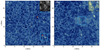 |
Fig. 1. Hε line core observations of a quiet Sun and pore region. The images are histogram equalized to the synthetic Hε line core image in Fig. 6. Left panel: quiet Sun observation with a wide band insert at the top right corner. The WB insert covers the area outlined by the light blue square and includes a few magnetic bright points. Right panel: more active scene close to a pore region (taken at 08:49:45 UT) with a zoomed-in insert at the top right corner (the insert is more saturated to highlight dark fibrils). Crosses indicate positions of spectral profiles shown in Fig. 2 with the same color coding. |
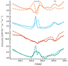 |
Fig. 2. Ca II H plus Hε spectral profiles for different solar structures indicated with crosses in Fig. 1. Solid lines: observations taken with the CHROMIS instrument. Dashed lines: degraded synthetic spectra. The Hε emission profiles are shown in orange and light blue. Orange synthetic profile (1.5D HNEI) is taken from Fig. 6 at x ≈ 13.6 Mm and y ≈ 17.7 Mm (red contours). Light blue synthetic profile (1.5D HNEI) shows the same as the one in the bottom right panel of Fig. 12. The red spectral profile is taken from a magnetic bright point. The synthetic profile (3D SE) is shown in the bottom left panel of Fig. 10. The turquoise spectral profile is taken from a dark fibrilar structure. The synthetic profile (1.5D HNEI) is shown in the bottom right panel of Fig. 10. |
We start with a discussion of where we are looking with regard to extinction in the quiet Sun case. The Hε line core images reveal a reversed granulation pattern. Reversed granulation originates from the mid-photosphere due to a reversal in the temperature structure, which leads to a reversal in the intensity images compared to the photospheric granulation pattern (Nordlund 1984; Cheung et al. 2007). The fact that the Hε line core image shows reversed granulation, as well as the Ca II H blue wing (see Fig. 3) suggests that the layers above reversed granulation are optically thin to Hε radiation. As we are looking at atmospheric layers close to the temperature minimum, the Hε extinction should be significantly reduced due to the temperature sensitivity of the hydrogen n = 2 population. A forward synthesis of Hε from the Bifrost simulation would help clarify which observed structures (if any) could be optically thick to Hε radiation. Furthermore, as no chromospheric canopy structure (the fibrilar chromosphere that is characteristic for a chromospheric line such as Hα) is apparent in Hε quiet Sun images, the chromosphere is mostly transparent, suggesting a mid-photospheric origin of Hε.
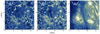 |
Fig. 3. Hε and Ca II H pore observation covering a region with stronger magnetic fields (taken at 09:17:52 UT). The wavelength positions are indicated in the top left corners on an average spectral profile with light blue crosses. Left panel: Ca II H blue (−0.15 nm) wing image, showing no chromospheric structures. Middle panel: Hε line core image, showing both reversed granulation and chromospheric structures. Right panel: Ca II H line core image, dominated by chromospheric structures. |
The pore region shows a slightly different picture. Here, we see some imprints of dark fibrilar structures. This hints at a chromospheric origin for such fibrilar structures observed in Hε (see top-right insert in the right panel of Fig. 1). To illustrate that Hε can show some chromospheric structures, we show the Ca II H blue wing, Hε, and Ca II H line core images side-by-side in Fig. 3. The blue wing Ca II H blue image shows only reversed granulation, whereas the Hε image shows fine imprints of dark fibrils. These dark fibrils are connected to chromospheric fibrilar structures observed in the Ca II H line core image, illustrating a chromospheric contribution in the Hε images. Not all dark fibrilar structures seem to be optically thick. Through some fibrilar structures, we observe the background with reversed granulation. In more active solar regions, the Hε extinction appears to increase at higher layers, making the chromosphere opaque. We note the images shown were taken during excellent seeing conditions, making the thin dark fibrilar structures clearly visible.
Next, we address the Hε source function. Ayres & Linsky (1975) suggested that the Hε source function is dominated by the Balmer continuum radiation field. This would result in apparent images resembling granulation if Hε is formed under optically-thick conditions, as the Balmer continuum is highly scattering and the thermalization depth lies in the photosphere. Nevertheless, we see reversed granulation in Hε images, which suggests most radiation is coming from the Ca II H background intensity and not Hε itself. Detailed radiative transfer calculations can reveal which hydrogen atomic transition dominates the Hε source function.
The conclusion we can draw from the Hε observations helps to narrow down the question, how the Hε line is formed in the solar atmosphere and gives some restriction on the total source function (Eq. (1)). The total source function  has to be sensitive to temperature but it is a linear combination of the line source function,
  , and the background source function,
  , weighted by their relative extinctions. This leaves us with two options. Either the Ca II H extinction dominates and
  is set by
  , which follows the Planck function. Or, instead, the Hε extinction dominates, and
  follows
  , which is coupled to temperature through one of the terms in Eq. (14).
We address the formation of Hε with the forward synthesis of Hε from state-of-the-art radiative MHD simulations. We specify where we are looking in the solar atmosphere in terms of extinction and determine the dominant processes in the total source function. We evaluate the effects of Balmer line blanketing, HNEI, and 3D effects on the formation of Hε. In addition, we discuss the appearance of bright points and elongated dark fibrils apparent in the Hε images with example spectra shown in Fig. 2 and why and when we see Hε in emission against the Ca II H background. We mainly focus on quiet Sun regions but will try to give some idea about the formation of Hε in more active regions.
4.2. Balmer continuum
The Balmer continuum radiation is the main driver of the hydrogen rate system and the dominant source of hydrogen ionization in the solar chromosphere (Carlsson & Stein 2002). Electrons recombine into high energy levels and cascade downwards, strongly affecting the transition rates and level populations of the hydrogen atom and, therefore, the Hε line. It is thus essential to properly model the Balmer continuum radiation field including line blends. RH 1.5D has the option to add line blends in the form of a Kurucz line list1. The spectral lines from the Kurucz line list are calculated assuming LTE, including scattering. To speed up the computation we created a list of lines that affect the Balmer continuum radiation significantly.
Figure 4 compares the synthesized Ca II H plus Hε spectral region from the FALC model atmosphere against the FTS atlas normalized to the continuum. The inclusion of line blanketing in the Balmer continuum results in stronger Hε absorption closely matching the observations. The bottom panel compares the FTS atlas against the average line profile summed over the Bifrost simulation calculated with SE and HNEI. There is a strong effect of the Balmer radiation field strength on the Hε line profile, but this does not necessarily mean that the Hε source function is set by the Balmer radiation field. It only highlights that the hydrogen transitions (as Hε) are sensitive to changes in the Balmer radiation field. To show that the Balmer radiation field sets the Hε source function, it is necessary to show that the divergence between the upper and lower level of Hε with height is set by the Balmer radiation field. Further, we have to evaluate what sets the total source function in Eq. (1) and which term dominates the multi-level source function in Eq. (14) for Hε.
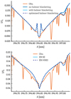 |
Fig. 4. Synthetic Ca II H and Hε spectral profiles compared against a FTS atlas observation. Top panel: FTS atlas observations (orange) compared to the synthesised Ca II H plus Hε profiles from the FALC model. Blue profile for the case with no Balmer continuum blanketing, light blue for Balmer blanketing with all lines included in the Kurucz line list, and dark blue for the optimized Kurucz line list including only lines affecting the Balmer continuum radiation significantly. Bottom panel: averaged Bifrost Ca II H plus Hε profiles for the SE (light blue) and HNEI (dark blue) case against FTS atlas observations (orange). |
Figure 5 presents what sets the total source function (top panel), the influence of the Balmer line blanketing on the total source function (middle panel), and what sets the Hε source function for the FALC solar-atmosphere model. The total source function is dominated by the Ca II H background source function throughout the lower solar atmosphere. At the formation height of Hε, only around 32% of the photons are actually from the Hε transition. This stems from the fact that Ca II H is a resonance line, whereas Hε lower level is an excited level with an energy jump of 10.2 eV. The Ca II H extinction will dominate the total extinction in the cooler parts of the atmosphere, with the dip in δ coinciding with the photospheric temperature minimum. This is an indication that the solar layers above reversed granulation are optically thin to Hε radiation.
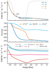 |
Fig. 5. Total source function of Hε, effect of Balmer continuum line blanketing, and Hε multi-level source function for the FALC model. Upper panel: line (SHϵ), background (Sb), and total source function (St), for the FALC model including Balmer continuum line blanketing. The dotted grey line shows the ratio δ between line extinction and total extinction (Eq. (2)). The three vertical ticks mark the total optical depth heights τλ = 3, 1, 0.3. The 32% label shows that at the τλ = 1 height 32% of the total source function consists of the Hε source function. Middle panel: fraction of the total, line, and background source function including Balmer blanketing and no Balmer blanketing. The change in the total source function with Balmer blanketing results from a change in the Hε source function, only making up 32% of the total source function. Bottom panel: Hε source function split up in the multi-level source function terms (Eq. (14); scattering |


The strong effect on the emergent Hε absorption stems from the Balmer line blanketing changing the total source function and not the extinction. The Balmer line blanketing has minor effects on the lower level populations of the Hε and Ca II H transitions that make up the extinction. As a result, the atmospheric layers we are looking at in the FALC model do not change, but the number of photons available as described by the source function does change. The middle panel illustrates that the change in the total source function, resulting from the Balmer line blanketing is mainly due to a change in the Hε source function – and not the background source function. Even when the total source function is dominated by the Ca II H source function. An increase in the strength of the Balmer radiation field (no Balmer blanketing) will lead to an increase in the upper-level population of the Hε transition, therefore, increasing the source function but keeping the Hε extinction the same. However, this does not show that the Hε source function is set by the Balmer radiation field, only that the Hε source function is somehow affected by the Balmer radiation field. To illustrate which process dominates the Hε source function we have to evaluate the multi-level source function.
The bottom panel of Fig. 5 divides the Hε source function into the multi-level source function terms. The contributions from the scattering  and thermal ϵB(Te) part are orders of magnitude lower than the one from interlocking ηB(Te). Interlocking dominates the Hε source function throughout the whole FALC model atmosphere. To highlight that the Hε source function is actually not following the Balmer radiation field we plotted the Balmer mean radiation field close to the Balmer edge in dotted green. The dominant interlocking term in Eq. (22) is
  , with the ground level as an intermediate level. The Planck function
  is set by the ratio P71q12, 7/P21q17, 2, where the probability q17, 2 characterizes the Hε source function. The probability q17, 2 represents the sum of the transition probabilities, p1i, Eq. (13) from the ground level into other hydrogen levels multiplied by the indirect transition probability to end up in the upper level of Hε. The transition probabilities are dominated by the radiative rates out of the ground level, not the collisional rates.
In summary, in the FALC model, the total source function is dominated by the Ca II H source function at the formation height of Hε. Our multi-level source function description suggests that the Hε source function is dominated by interlocking, with the ground level being the dominant intermediate level radiatively populating the upper level of Hε and not by the Balmer continuum radiation field as suggested by Ayres & Linsky (1975).
4.3. Effect of HNEI on Hε
The solar chromosphere is pervaded by upwardly propagating magneto-acoustic shocks, making the effect of time-dependent hydrogen ionization important already above the solar photosphere. Non-equilibrium computations of hydrogen ionization strongly affect the temperature structure and ionization of the atmosphere due to the slow recombination rate at low-temperature intershock phases (Leenaarts et al. 2007). The ion population in turn is strongly coupled to the n = 2 population of hydrogen, which sets the line extinction of Hε and therefore the formation height of Balmer series lines (Carlsson & Stein 2002). In some cases, HNEI can have strong effects depending on where we are looking at in the atmosphere and what we are observing, thereby directly influencing the Hε source function.
Figure 6 shows synthesized Hε line core (at 397.1202 nm) images from the Bifrost simulation (left panel for SE, and right panel for HNEI). The SE case uses the standard version of RH to solve the statistical equilibrium equation, which loses information about the time-dependent hydrogen ionization. Our HNEI implementation in RH uses the proton density given by the Bifrost simulation (see Sect. 3.5).
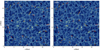 |
Fig. 6. Synthetic Hε line core images at 397.1202 nm. Left panel: SE case. Right panel: HNEI case. Contours mark regions of Hε emission at different column mass regions. Yellow: column mass ≥2 × 10⁻¹ g cm−2. Red: 2 × 10⁻¹ g cm−1 > column mass > 2 × 10⁻² g cm−2. Cyan: column mass ≤ 2 × 10⁻² g cm−2. Dashed lines: position of the vertical slice shown in Fig. 7. |
The two images look almost identical. Both are mapping reversed granulation, which originates in the mid-photosphere. The synthetic images match the observed Hε images from Fig. 1 quite well, which suggests a similar formation of Hε between simulation and observations. However, the effect of HNEI seems negligible for the observed reversed granulation pattern, which in the simulation is mainly made up of weak Hε absorption lines. To evaluate the effect of HNEI on the Hε source function and extinction, we look at a vertical cut through the Bifrost simulation, denoted by two dashed lines in Fig. 6.
Figure 7 compares the hydrogen ionization structure and n = 2 level population for the cases of SE and HNEI. The HNEI case shows a different and smoother ionization structure through the atmosphere compared to the SE case. This is also reflected in the n = 2 populations – especially in the lower part of the atmosphere (below 1 Mm), where the dark voids vanish under HNEI. The reason for the smoother n = 2 populations is that under HNEI the n = 2 populations follow the hydrogen ionization (Leenaarts et al. 2007), whereas for SE, the n = 2 population follows the temperature (compare temperature panel in Fig. 8). This temperature sensitivity below 1 Mm stems from the fact that Lyman-α is in radiative balance n1/n2 = R21/R12 with S ≈ J ≈ B. Therefore, the n = 2 hydrogen population follows LTE: Saha-Boltzmann partitioning for the predominately neutral lower solar atmosphere, with high Lyman-α extinction (Vernazza et al. 1981; Rutten 2016, 2017).
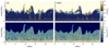 |
Fig. 7. Hydrogen ionization (top) and n = 2 populations (bottom) from a vertical slice through the simulation (indicated in Fig. 6). Left column: results for statistical equilibrium (SE). Right column: results for non-equilibrium hydrogen ionization (HNEI). The solid orange and dashed grey lines show the τ = 1 heights for both cases, and the orange crosses and light blue crosses mark regions where Hε is in emission. The dark blue line shows the relative variation of the Hε line core intensity. |
The n = 2 level population increases strongly for hot pockets in the lower solar atmosphere in SE. This raises the τ = 1 height, represented by the orange line in Fig. 7. These elevated τ = 1 locations are connected to Hε emission indicated by crosses. Under HNEI the Hε extinction does not “feel” this temperature increases as much as in SE. This not only has a strong influence on the extinction but also on the source function itself. The influence of HNEI on the n = 2 populations and total source function in terms of departure from SE can be seen in Fig. 8. We show the departures from SE for the lower solar atmosphere in the formation region of Hε. The τ = 1 heights for Hε, where most of the radiation escapes are similar between SE and HNEI, which illustrates that the increase in the n = 2 populations under HNEI is not enough to change where we are looking at in the simulation. Further, the total source functions at the τ = 1 height do not change much between SE and HNEI. Therefore, time-dependent hydrogen ionization effects are negligible for the Hε extinction and the total source function where Hε absorption is formed. However, this is not the case for Hε emission.
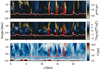 |
Fig. 8. Departures from statistical equilibrium from a vertical slice through the Bifrost simulation. Top panel: departure of the total source function from SE. Middle panel: departure of the hydrogen n = 2 populations from SE. Bottom panel: temperature structure of the Bifrost simulation. The vertical slice is taken at the position marked with white dashed lines in Fig. 6. Red solid: Hετ = 1 height for SE. White dashed: Hετ = 1 height for HNEI. |
Hε emission is co-located with enhanced temperatures in the lower solar atmosphere, as illustrated in the lower panel of Fig. 8 (Hε emission is marked with crosses in Fig. 7). This leads to two orders of magnitude higher n = 2 populations at these heating events, shifting up the τ = 1 formation heights. At these particular atmospheric heights, the total source function under SE is significantly higher (up to a factor of 2) compared to HNEI, resulting in stronger Hε emission. Only two out of five emission locations (crosses in Fig. 7) are still in emission in HNEI. Even though the τ = 1 height is lower in HNEI, for these two locations in emission, under SE, the Hε emission profile has a significant contribution from these higher-lying layers, where the total source function is increased.
HNEI has a sizeable effect on the n = 2 populations throughout the whole atmosphere, from the lower atmosphere up to the transition region. It changes not only the extinction but also the Hε source function. This effect can be seen in Fig. 8 (top panel). Similarly, we find that HNEI also affects the line source functions of other lines in the Balmer series (not shown in the figures). Depending on where the lines are formed, the difference between the emergent Balmer series line profiles in SE or HNEI can be significant. Another important side effect of HNEI is time-dependent ionization, where the hydrogen populations can have a memory of a previous atmospheric state, decoupling the observed line profiles from the instantaneous conditions in the atmosphere. This has implications for the interpretation of Hα spectroheliograms, as they contain information about previous events, especially heating events that increase the Hα extinction (Rutten 2016).
The strong effect of HNEI on Hε emission can be seen in Fig. 6, where the over-plotted contours mark regions where Hε is in emission. The different colored contours group the column masses at τ = 1 height into three different groups related to the column mass panel of Fig. 9. The yellow contours highlight regions where the column mass at τ = 1 is greater than or equal to 2 × 10⁻² g cm−1, red regions greater than 2 × 10⁻¹ g cm−2 and less than 2 × 10⁻² g cm−2, and the cyan color less than or equal to 2 × 10⁻² g cm−2. Figure 9 shows a kernel density estimation (Rosenblatt 1956) for the distributions of formation heights, column masses, temperatures, and electron densities at the τ = 1 heights for Hε emission and absorption lines for the Bifrost simulation. Hε in absorption is formed just above the Ca II H background, whereas Hε emission is formed across a large range of column masses. This range is connected to enhanced temperatures in the lower solar atmosphere, which shifts the formation height upwards under SE and is connected to increased ionization in HNEI. Generally, HNEI reduces the amount of Hε emission formed higher up in the atmosphere.
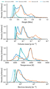 |
Fig. 9. Distributions of atmospheric quantities at the Hετ = 1 height. Panels show the kernel density estimation as a function of height, column mass, temperature, and electron density at the τ = 1 height for the Hε rest wavelength. The distributions are separated by the type of Hε profile, as indicated in the legend: absorption in HNEI, emission in HNEI, emission in SE, and the Ca II H background continuum at Hε rest wavelength in HNEI. |
In summary, Hε synthetic images are similar to solar observations, showing mainly reversed granulation. Why we observe reversed granulation in the Hε line core, we will address in the Sect. 4.4. Furthermore, we have to explain the small bright points seen in the Hε line core images; HNEI has little effect on the reversed granulation pattern but influences the Hε emission. As Hε emission can form relatively high up in the lower solar atmosphere, we have to check for probable 3D radiative transfer effects (Sect. 4.5).
4.4. Hε absorption
In this section, we discuss the formation of Hε absorption profiles. We analyze why we observe reversed granulation in weak Hε absorption profiles and why strong Hε absorption lines are linked to magnetic elements.
Figure 10 shows a synthetic Hε line core image from a small region from the Bifrost simulation. The region covers a magnetic element and parts of the reversed granulation pattern. To check for 3D effects we synthesized the same region in 3D, but assuming SE and treating Ca II H in CRD. We adopted these approximations because it was difficult to get RH to converge under HNEI and PRD in regions with strong horizontal inhomogeneities, such as magnetic elements. Representative profiles are shown in Fig. 10 including one particularly interesting structure, which goes from Hε emission in 1.5D to absorption in 3D (this structure crosses the red cross at an approximately 45° angle). We address the effects of 3D radiative transfer on Hε emission in Sect. 4.5.
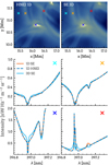 |
Fig. 10. Synthetic Ca II H and Hε images and spectral profiles for reversed granulation, magnetic elements, and a dark fibrilar structure. Topmost row: synthesized Hε line core images from a cutout of the Bifrost simulation calculated in 1D (left) and 3D (right). Bottom two rows: Ca II H plus Hε spectral profiles from locations marked with coloured crosses in the Hε line core images. Middle-left: granular spectral profile. Middle-right: intergranular spectral profile. Bottom-left: spectral profile located at a magnetic field concentration. Bottom-right: location where Hε emission in 1D turns to absorption in 3D. |
In general, we observe very weak Hε absorption lines inside granules that get stronger the closer we get to the granular edge. 3D effects are negligible on the Hε line profiles (see middle panels of Fig. 10). To discuss the formation of weak Hε absorption lines we created relative four-panel formation diagrams inspired by Carlsson & Stein (1997). Figure 11 displays such diagrams, which we henceforth refer to as “four-panel diagrams”. The four-panel diagrams decompose the contribution to relative line depression or emission into three components:
 (26)
(26)
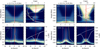 |
Fig. 11. Hε four-panel diagrams for an intergranular lane (left) and a magnetic bright point (right). The locations of each point in the simulation are marked with orange and blue crosses in Fig. 10. Each diagram is organized as follows. Top left panels: relative χν/τν; sensitive to velocity gradients. Top right panels: Sν: relative source function. Solid white: total source function at rest wavelength. Dashed yellow: Hε source function. Dashed blue: background source function. Source functions are displayed in brightness temperature units with the scale at the top. Solid grey: ratio of Hε to total extinction (if Hε extinction dominates the grey curve is on the left side of the plot; if Ca II H extinction dominates on the right). Dotted red: atmospheric temperature profile. Bottom-left panels: relative τνe( − τν); indicates where most of the contribution to relative line intensity comes from. Solid green: ϵBν(Te). Solid violet: σJν. Solid gold: ηBν(T⋆). The three terms are displayed in brightness temperature units with the scale at the top. Bottom-right panels: CI; contribution to relative line depression. Solid white: Ca II H plus Hε line profile. Dashed white: Ca II H background line profile. Solid red: atmospheric vertical velocity profile. Solid light blue: τ = 1 height. |
based on Eq. (5). The first component  is the ratio between relative extinction and relative optical depth. This term has large values where there are many absorbing or emitting particles (line and background;
  ) at low relative optical depth. This component is sensitive to line-of-sight velocity gradients that move plasma, so that they effectively increase extinction at varying Doppler offsets at wavelength regions with low optical depths.
The second component  has the largest values around the τ = 1 height. In this panel, we over-plotted the three components of the multi-level source function (Eq. (14)) for Hε. This helps to determine the dominant line-formation process.
The third component  (z) describes the relative source function. The relative source function can have positive or negative values. This is a major difference from standard four-panel formation diagrams, where the source function panel only has positive values. Here, positive values signify that the line source function,
  , is lower than the background intensity,
  , resulting in a contribution to relative line depression at a particular height in the atmosphere. Negative values signify a relative contribution to line emission. However, the relative source function does not specify what sets the total source function at the formation height of Hε. Based on the upper panel of Fig. 5, we included the different components expressing the total source function at the Hε line core wavelength: the total source function, the Hε source function, the background source function, and additionally included the ratio of Hε extinction to total extinction. The last panel shows CI, which is the contribution to the relative line depression or emission. We note that CI is positive in regions that contribute to line absorption and negative in regions that contribute to line emission.
First, we focus on the left four-panel diagram in Fig. 11, which illustrates the formation of a relatively weak Hε absorption line in the intergranular lane (orange cross in Fig. 10). Most contribution to relative line depression is formed just above the Ca II H background intensity. This highlights that the added Hε extinction on top of the Ca II H extinction is very small, making the atmosphere nearly transparent to Hε radiation. Further, we have to evaluate what sets the total source function at the line formation region specified by the relative extinction over-plotted in the relative source function panel. The grey curve points out that more than 50% of line photons are actually coming from the Ca II H transition. The total source function is more tightly coupled to the Ca II H source function than to the Hε source function. The Ca II H source function is still strongly coupled to LTE, which means that in this case more than 50% of photons at the Hε wavelength are formed under LTE conditions. The optical depth τλ of the atmosphere above the height where the Ca II H background is formed is just below unity (τ ≈ 0.78 for the intergranular location), thus giving the appearance of reversed granulation in the Hε line core, which happens for most for quiet Sun locations.
The closer we get to the granular center, the weaker the Hε absorption gets (see the middle row in Fig. 10). This stems from the fact that the mid-photosphere is cooler at the center of granules where reversed granulation is formed. As the Hε extinction is strongly coupled to Saha-Boltzmann due to Lyman-α thermalization, the Hε contribution to the total extinction becomes smaller, essentially removing the Hε line depression. The decrease in Hε extinction will couple the total source function even closer to the Ca II H source function (≈80%).
The change in Hε absorption strength from the granular center to the granular edge is therefore dependent on the temperature structure and not so much on the strength of the Balmer radiation. The Balmer radiation will indeed increase the Hε source function in both SE and HNEI. In SE, a stronger Balmer radiation field will not change the Hε extinction (n = 2 population), but increase the n = 7 populations, thereby increasing the Hε source function. In HNEI, the behavior is different: the Hε extinction and n = 7 populations decrease for a stronger Balmer radiation field but still result in an increased Hε source function as the Hε extinction decreases more rapidly with height than the n = 7 populations. However, the Hε source function for weak Hε absorption is dominated by interlocking illustrated by the gold solid line in the  panel. Similarly, as in Sect. 4.2, our multi-level source function description suggests the interlocking term is dominated by the Lyman series with indirect transitions into the upper level Hε through the ground level – and not by the Balmer radiation field. The Balmer radiation field will affect the mean radiation fields in the Lyman series, but not the Hε source function directly.
We now move to the formation of strong Hε absorption lines. As a representative example, we consider the bottom left line profile in Fig. 10 (blue cross), and show its corresponding four-panel diagram in Fig. 11 (right panels). This strong Hε absorption line is connected to a magnetic field concentration. Due to the low gas density inside magnetic elements, Hε forms at lower heights, therefore, it is associated with higher temperatures. As the Ca II H wing intensity is well approximated by LTE and follows the temperature, the intensity above the magnetic elements will be significantly increased compared to that in reversed granulation. The reason is similar to why magnetic elements appear bright in the wings of Hα (Leenaarts et al. 2006). However, Hε is formed on top of the Ca II H wing. The added Hε extinction shifts the formation height upwards making magnetic elements optically thick to Hε radiation. The total source function strongly decreases with height, being mainly set by the Hε source function due to the increased Hε extinction above magnetic elements. This mapping of higher layers with a lower source function compared to the Ca II H background leads to strong Hε absorption lines. Therefore, Hε can be used to identify and track weak magnetic elements.
Our multi-level source function description also suggests that the Hε source function is dominated by interlocking. The dominant interlocking process is an indirect transition loop through the ground level for strong Hε absorption profiles connected to magnetic field concentrations, the same process as found for weak Hε absorption profiles.
The fourth profile, marked with a red cross in Fig. 10 is a good example that some Hε profiles can suffer significant 3D effects. In this particular case, the bright elongated structure seen in 1D will turn into a faint fibrilar structure if 3D radiative transfer effects are taken into account. In the next section, we address 3D effects on Hε emission regions, where the formation height is increased compared to the usual reversed granulation.
4.5. 3D effects on Hε emission
The Balmer series lines, for example Hα, are strongly affected by scattering. The characteristic fibrilar chromosphere seen in Hα can only be reproduced if the radiation field is treated in 3D geometry (Leenaarts et al. 2012b). However, as shown in Sect. 4.2, the Hε source function is not dominated by two-level scattering but instead by interlocking through the Lyman series. The Lyman series lines are the strongest scattering lines in the solar spectrum, having the lowest collisional destruction probability per line photon extinction. Hence, we evaluated 3D Lyman scattering effects on the emergent Hε line profiles formed higher up in the atmosphere (at lower column masses than 2 × 10⁻² g cm−2).
To investigate 3D effects on the emergent Hε profiles, we chose small regions of interest from the Bifrost simulation. From these regions, we synthesized Hε with the assumption of HNEI in 1D and 3D geometry. We carried out spectral synthesis in 3D only in these selected regions to avoid the large computational costs of a full 3D synthesis, and because there are only a few regions where Hε is formed higher up in the atmosphere. Furthermore, we synthesized Ca II H in CRD instead of PRD in 3D geometry as the running with PRD led to numerical instabilities and the problem often failed to converge. Because we assume CRD in 3D, the intensity at the Ca II H inner wings will deviate between 3D and 1.5D.
First, we discuss the case of low column mass, where 3D effects become important at certain locations. Figure 12 shows two regions of interest from the Bifrost simulation, where Hε is in emission at low column mass. The left column shows a region with strong 3D effects, while the right column shows a region with negligible 3D effects. We show the corresponding four-panel diagrams in Fig. 13.
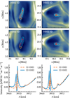 |
Fig. 12. Synthetic Ca II H and Hε images and spectral profiles for Hε emission formed at low mass densities. Top two rows: synthesized Hε line core images from a cutout of the Bifrost simulation calculated in 1D (top row) and 3D (middle row). Contours mark column mass regions, same as in Fig. 6. Bottom row: Ca II H plus Hε spectral profiles from locations marked with red crosses in the Hε line core images. |
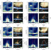 |
Fig. 13. Hε four-panel diagrams for the locations marked with crosses in Fig. 12. Top row: Hε synthesized in 1.5D. Bottom row: same location synthesized in 3D. Top left panels: relative χν/τν; sensitive to velocity gradients. Top right panels: Sν; relative source function. Yellow colormap for negative source function values. Light blue colormap for positive source function values. Solid white: total source function at rest wavelength. Dashed yellow: Hε source function. Dashed blue: background source function. Source functions are displayed in brightness temperature units with the scale at the top. Solid grey: ratio of Hε to total extinction (if Hε extinction dominates the grey curve is on the left side of the plot; if Ca II H extinction dominates on the right). Dotted red: atmospheric temperature profile. Bottom left panels: relative τνe( − τν); indicates where most of the contribution to relative line intensity comes from. Solid green: ϵBν(Te). Solid violet: σJν. Solid gold: ηBν(T⋆). The three terms are displayed in brightness temperature units with the scale at the top. Bottom right panels: CI; contribution to relative line depression/emission. Yellow colormap contribution to line depression. Light blue colormap contribution to line emission. Solid white: Ca II H plus Hε line profile. Dashed white: Ca II H background line profile. Solid red: atmospheric upward velocity profile. Solid light blue: τ = 1 height. |
The left column of Fig. 13 illustrates the formation of Hε with strong 3D effects. In the 3D case, CI outlines significantly more contribution to line depression than for the 1.5D case on top of the relative line emission region. The answer to the question of why we have more contribution to line depression in 3D is twofold. First the Hε extinction  plays an important role (see Eq. (8)). The n = 2 populations are in radiative equilibrium with Lyman-α as n2 = n1R12/R21 is set by the Lyman-α mean radiation field and the exponential density decrease of the atmosphere. The Lyman-α mean radiation field in 3D is slightly increased compared to 1.5D. Therefore, the Hε extinction is mapping more of the positive relative source function giving rise to relative line depression. However, the increase in Hε extinction is not the main reason for the enhanced contribution to the relative line depression in 3D highlighted by similar τνexp(−τν) panels.
The main reason why we see enhanced relative line depression in 3D is that the Hε line source function is significantly lower than the 1.5D case above a certain atmospheric height. This decrease in  in 3D causes a negative relative line source function at lower heights compared to 1.5D (illustrated in the top right Sν panels in Fig. 13). The relative source function becomes negative when the Hε source function
  is smaller then the background Ca II H wing intensity, specified by
  . The background intensity
  flattens out with height (around ≈0.5 Mm), having lower values in 3D. Our multi-level source function description suggests that the Hε source function is dominated by interlocking, set by the Lyman series (same process as for Hε absorption), or more precisely, a linear combination of the transition probability, p1i, multiplied by an indirect transition probability, qi7, 2, due to a Lyman series transition. The transition probabilities are dominated by the radiative rates. The net rate out of the ground level is set by the Lyman-α radiative rate which is orders of magnitude higher than other Lyman series radiative rates. Therefore, the transition probabilities are given by p1i = R1i/R12 and reflect the ratio between the Lyman series and the Lyman-α mean radiation field. The main difference between 1.5D and 3D is that this ratio decreases more strongly with height in 3D than in 1.5D. This puts the Hε source function,
  , below the Ca II H background intensity,
  , at lower heights giving rise to a negative source function creating the strong relative absorption contribution in 3D.
The negligible 3D effects on Hε for the right column of Fig. 13 stem from the fact that the temperature increase is situated lower in the atmosphere than for the left column. This temperature rise at lower heights leads to a coupling of the Lyman-α mean radiation field with the Planck function to heights where the temperature is decreasing again, above the temperature peak. Whereas for the case of strong 3D effects, the Lyman-α mean radiation decouples from the Planck function at the temperature peak in the atmosphere. In both cases, the Lyman-α mean radiation decouples approximately at the same height from the Planck function. As the n = 2 level population follows the Lyman-α mean radiation via n2 = n1R12/R21, the Hε line extinction  decreases after the temperature rise. This strong decrease in line extinction, as illustrated in the τνexp(−τν) panel, is the main reason why we do not see a strong contribution to relative line depression above the emission region. The Hε emission formed at greater column masses than 2 × 10⁻² g cm−2 (yellow and red contours in Fig. 6) show negligible 3D effects.
In summary: if a temperature increase in the lower solar atmosphere extends too high up in the atmosphere and is not confined in the lower solar atmosphere (for the Bifrost simulation this would be approximately a height of 0.75 Mm), the Hε line will suffer from 3D effects, showing a Hε absorption line instead of a Hε emission line in 1.5D, given the density stratification of the Bifrost atmosphere.
This explains the strong change in the appearance of the bright fibrilar structure in 1.5D in Fig. 10, compared with the dark fibrilar structure seen in 3D. Figure 8 show a temperature cut through this fibrilar structure (white dashed lines in Fig. 6). The strong temperature enhancement throughout the lower atmosphere connected to this structure leads to an increased Hε line extinction via n2 = n1R12/R21. The 3D effects lead to a lower Hε line source function than the Ca II H background intensity  and give a strong contribution to relative line depression above the emission region compared to the 1.5D case. As a result, the 1.5D Hε emission lines at the fibrilar structure become absorption lines in 3D.
5. Discussion
5.1. The Hε source function
Numerical experiments such as the Bifrost simulation represent a solar-like model atmosphere with properties close to the real solar atmosphere. We focus our discussion on the similarities between synthetic and observed Hε profiles. The synthetic Hε profiles combined with the Bifrost simulation can help us understand the basic formation processes in the solar atmosphere that lead to features observed in the quiet Sun, such as reversed granulation, bright points, Hε emission, and dark fibrilar structures.
Several decades ago, Thomas (1957) suggested dividing the resonance lines and strong lines such as Hα into collisionally or photoelectrically dominated. For Hα, this division meant that the source function is set by collisions, the second term in Eq. (14), or by the third term (photoelectric) in Eq. (14). The third term describes the interlocking contribution to the line source function and, following Thomas (1957), it states that the indirect path that dominates the Hα source function is photoionization from n = 2 and a recombination cascade into n = 3 (thus, the description of it as photoelectric). However, Rutten & Uitenbroek (2012) demonstrated that the Hα source function is dominated by scattering, described by the first term in Eq. (14), with strong contributions from chromospheric backscattering. However, our main question concerns which process dominates the source function of higher order Balmer series lines, such as Hε.
Ayres & Linsky (1975) first modeled the formation of Hε based on 1D numerical radiative transfer calculations for two model atmospheres, one representing the Sun (Hε in absorption) and one Arcturus (Hε in emission). They concluded that the Balmer continuum radiation dominates the Hε source function via photoionization, the same mechanism proposed by Thomas (1957) for the Hα source function. However, our Hε forward modeling from the FALC and Bifrost model atmosphere suggests otherwise. Our multi-level source function description suggests that the Hε source function is dominated by interlocking via the ground level of hydrogen due to the Lyman series. Not the Balmer continuum radiation field.
Our synthetic Hε line core images (Fig. 6) reproduce the observed Hε reversed granulation pattern (Fig. 1) quite well. Both show the characteristic dark granules and bright intergranular lanes suggesting that the Bifrost simulation has the basic physical properties representing a quiet Sun lower atmosphere. The reversed granulation pattern consists of weak Hε absorption lines. The weakest Hε absorption profiles can be found inside granules and the closer we get to the intergranular lanes, the stronger the Hε absorption becomes. We illustrated that the total source function for weak Hε absorption lines is dominated by the background Ca II H source function and not the Hε source function. The temperature structure of the reversed granulation sets the extinction and total source function and therefore the behavior of weak Hε absorption lines.
We tested the influence of HNEI on the emergent Hε line profiles against SE. The influence is negligible at the reversed granulation pattern, which is represented by weak Hε absorption lines, formed deep in the solar atmosphere where time-dependent ionization is not important. However, for hydrogen lines formed higher up in the solar atmosphere, HNEI will have severe effects on the line extinctions and source functions. The main effect of HNEI is that the proton density sets the level populations and not the temperature structure. Therefore, structures not reflecting reversed granulation should indicate high ionization regions (leading to increased extinction), showing higher atmospheric layers than reversed granulation. The most prominent features seen sticking out of the reversed granulation background in Figs. 1 and 3 are bright points and dark fibrilar structures.
5.2. Bright points
The bright points in our synthetic and observational Hε images are connected to small magnetic elements. The wide band insert in Fig. 1 illustrates that the magnetic structures are connected to Hε bright points. We explained the formation of Hε above magnetic elements in Sect. 4.4 as the result of density depletion and a different optical depth scale compared to their surroundings. Therefore, we get large Ca II H wing intensities (formed under LTE) with strong Hε absorption lines on top. The strong Hε absorption forms higher in the atmosphere, with a strong decrease of the total source function versus height that is dominated by the Hε source function. If we compare our synthetic Hε profile in Fig. 2 with observations of a magnetic element (red profiles), they look remarkably similar. Therefore, we conclude that bright points in Hε observations represent magnetic elements where the Ca II H wing intensities reflect the temperature at the Ca II H wing formation height, and the strong Hε absorption lines reflect an enhanced Hε extinction above magnetic elements where the Hε source function drops rapidly with increasing height.
5.3. Dark fibrilar structures
We could only reproduce a dark fibrilar structure with the Bifrost simulation if we include 3D radiative transfer effects; still, these structures are rare in the synthetic spectra. One example is shown in Fig. 10, where the bright fibrilar structure in 1D turns into a (very faint) dark fibrilar structure if 3D effects are taken into account. This feature goes diagonally through the red cross in Fig. 10, extending nearly to the top and right borders of the image. The 3D radiative transfer effects lead to stronger relative absorption contribution above emission (see Fig. 13) compared to 1D. The reason is the temperature structure of the atmosphere. The temperature structure (or proton densities under HNEI) sets the n = 2 populations due to the Lyman-α mean radiation field. If we have high-enough temperatures in the lower atmosphere, up to heights where the Lyman-α decouples from the Planck function, it will increase the Hε line extinction. This increases the contribution from higher layers, where the Hε source function is lower than the Ca II H background intensity, thereby giving rise to strong contributions to absorption. Such dark fibrilar structures could in principle be visible in solar observations and not only in synthetic Hε images from simulation. They would mark regions with strong heating: high temperatures that extend from the lower atmosphere up to the lower chromosphere and are not confined to the lower atmosphere.
It is important to avoid confusing the Bifrost dark fibrilar structure shown in Fig. 10 with the dark fibrilar structures observed in more active regions (Fig. 3). These fibrilar structures become partly opaque due to increased mass density similar to the Hα fibrilar chromosphere (Leenaarts et al. 2012b). These fibrilar structures outline the chromospheric canopy. There is a clear correlation between the dark fibrilar structures seen in the Ca II H and Hε line core images. On the other hand, the dark fibrilar structure from Bifrost is a result of heating. Dark fibrilar structures similar to those seen in the simulation should be observable in the quiet Sun, but they may be easily confused with other dark structures connected to the reversed granulation background. Dark fibrilar structures should stand out clearly from the Ca II H reversed granulation and not be aligned with the reversed granulation pattern. One example of this is the dark fibrilar structure seen in Fig. 10 connecting two different granules. It is conceivable that a strong episode of flux emergence may be an event that shows clear signatures of dark fibrilar structures.
5.4. Hε in emission
Lastly, we address locations of Hε emission that mark regions of confined heating in the lower atmosphere (otherwise 3D effects would become important and we would observe a Hε absorption line). Locations with Hε in emission are difficult to identify only by looking at Hε line core images. We have to look at the individual line profiles to identify locations with emission. In Fig. 6, we outlined Hε emission locations with contours. All locations covered by contours in the simulation are related to temperature enhancements in the lower atmosphere, at heights between 0.3 Mm and 0.75 Mm in the Bifrost simulation (see an example in Fig. 13). We found a significant amount of Hε emission in the Bifrost simulation, but a question arises about whether such emission can also be found in observations covering quiet Sun regions, as Hε is generally thought to be a weak absorption feature in the quiet Sun. To illustrate that the quiet Sun does show regions with emission, we show two example profiles in Fig. 2 and compare them to some of our synthetic profiles.
Observing Hε in emission requires high resolution. We interpret the regions with Hε emission as locations marking confined heating events: weak temperature enhancements in the lower solar atmosphere, as illustrated by the formation of Hε emission from the Bifrost simulation. We are not aware of any spectral line that shows such a clear signature of weak small-scale heating (≈6000 K) in the lower solar atmosphere. The Mg II triplet lines are sensitive to such weak heating events formed at even lower column masses (Pereira et al. 2015) and can serve as a fitting complement to Hε.
6. Conclusions
We revisited the formation of Hε, inspired by the work of Ayres & Linsky (1975), and we propose that the Hε source function is not set by the Balmer radiation field but instead by interlocking via the ground level. We present high-resolution Hε line core images that appear to be dominated by reversed granulation, mostly coming from the Ca II H background radiation as the contribution of Hε is very small under typical quiet Sun conditions. In several cases, we find locations with a different appearance: bright points or dark fibrilar structures that are related to enhanced temperatures and reflect locations where a majority of photons come from the Hε transition. These structures are optically thick to Hε radiation. Therefore, Hε line core images represent a stacked view of different atmospheric layers where the dominant source of photons varies with hydrogen ionization.
Our main findings are as follows:
-
In most quiet Sun locations, the Hε extinction is minor and the atmospheric layers above the formation height of Ca II H are transparent to Hε radiation.
-
In magnetic elements and small-scale heating events, the Hε extinction dominates and the atmospheric layers are optically thick to Hε radiation.
-
Our multi-level source function description suggests that the Hε source function is dominated by interlocking via the term P71q12, 7/P21q17, 2, with the hydrogen ground level as intermediate interlocking level – and not by the Balmer continuum radiation.
-
The Hε source function is dominated by the Lyman series via the term q17, 2, which represents a linear combination of the transition probabilities out of the ground level.
-
The Hε source function and extinction are both coupled to temperature in the lower solar atmosphere. The extinction via Lyman-α, and the source function via the whole Lyman series.
-
HNEI couples the hydrogen populations to the proton densities, whereas SE couples the population to temperature in the lower solar atmosphere. HNEI has a strong effect on all hydrogen lines, affecting both source functions and extinctions.
-
We can synthesize Hε in 1.5D with the assumption of HNEI as long as Hε is not formed too high up in the atmosphere, where the 3D effect can become important.
-
HNEI has the strongest effect at locations where Hε is formed higher up in the solar atmosphere, such as magnetic elements, dark fibrilar structures, and Hε emission locations.
-
Hε emission marks locations of confined heating events in the lower solar atmosphere.
The Hε transition is special compared to Hα and Hβ because the extinction and source function are coupled to temperature. For Hα and Hβ, only the extinctions are coupled to temperature, while their source functions are dominated by scattering, except by strong heating events in the lower atmosphere such as Ellerman bombs (Ellerman 1917; Rutten et al. 2013). In Hα and Hβ, the line core extinction is high enough that we observe the chromospheric magnetic canopy. For Hε, this is not the case. This gives the unique opportunity for a Balmer series line to look through the magnetic canopy and observe heating events in the lower solar atmosphere. Another interesting fact is that the source function of higher-order Balmer series lines (higher than Hα and Hβ) seem to become dominated by interlocking via the Lyman series, and therefore temperature-sensitive. This extinction “gap” and temperature sensitivity of the Hε source function opens a new window onto the possibility of observing small-scale weak heating events in the lower atmosphere marked by Hε emission regions, for instance, QSEB reconnection events (Rouppe van der Voort et al. 2016; Joshi et al. 2020), shocks, and others in high spatial and temporal cadence. Another positive aspect is that it is relatively easy to observe Hε together with Ca II H. For example, the CHROMIS instrument at the SST can observe both lines without sacrificing too much temporal cadence making the combination of spectral lines a strong diagnostic tool. The Hε and Ca II H combination is also well covered by the ViSP instrument (de Wijn et al. 2022) at DKIST (Rimmele et al. 2020).
The Hε line is not only of solar interest but also for the wider astrophysics community. Generally, Hε is used to study stellar flare activity (Pavlenko et al. 2019), chromospheric activity in M and K dwarfs (Houdebine et al. 2009; Maldonado et al. 2017), active galactic nuclei (AGNs; Ilić et al. 2012), young active stars (Biazzo et al. 2009), Cepheids (Kovtyukh et al. 2015), and chromospheric active binaries (Montes et al. 1995, 1996). Montes et al. (1996) showed a clear surface flux correlation between Ca II H and Hε excess emission for chromospherically active binaries. We can explain this correlation qualitatively. The Ca II H source function for these types of stars is collisionally dominated, formed under LTE conditions, and therefore the intensity is proportional to temperature. Meanwhile, the Hε source function is set by interlocking with a partial sensitivity to temperature and therefore the intensity is coupled to the temperature structure of the atmosphere. The sensitivity of both lines to temperature results in a strong correlation between the two line excess fluxes and explains the steep temperature increase needed to produce Hε emission against the Ca II H background intensity.
We demonstrate that the Hε can be used to detect weak small-scale heating in the lower solar atmosphere at an unprecedented resolution. This could be of particular interest in the studies of QSEBs and it is worthwhile exploring how Hε could help to shed light on these new phenomena in greater detail. Further questions that ought to be considered in future studies include: what higher order Balmer series lines can tell us about QSEBs and whether stellar Hε emission forms the same way as in the solar atmosphere as we have predicted, as well as when (and why) the Balmer series lines actually become dominated by interlocking.
For details see: http://kurucz.harvard.edu/linelists.html
Acknowledgments
This work has been supported by the Research Council of Norway through its Centers of Excellence scheme, project number 262622, and through project number 325491. Computational resources have been provided by Sigma2 – the National Infrastructure for High-Performance Computing and Data Storage in Norway. We acknowledge funding support by the European Research Council under ERC Synergy grant agreement No. 810218 (Whole Sun). K.K. acknowledges the insight Mats Carlsson gave during his Stellar Atmospheres II course. The Swedish 1-m Solar Telescope is operated on the island of La Palma by the Institute for Solar Physics of Stockholm University in the Spanish Observatorio del Roque de los Muchachos of the Instituto de Astrofísica de Canarias. The Institute for Solar Physics is supported by a grant for research infrastructures of national importance from the Swedish Research Council (registration number 2021-00169). The Scientific color maps (Crameri 2021) are used in this study to prevent visual distortion of the data and exclusion of readers with colour vision deficiencies (Crameri et al. 2020).
References
- Anan, T., Ichimoto, K., & Hillier, A. 2017, A&A, 601, A103 [NASA ADS] [CrossRef] [EDP Sciences] [Google Scholar]
- Ayres, T. R., & Linsky, J. L. 1975, ApJ, 201, 212 [NASA ADS] [CrossRef] [Google Scholar]
- Bayazitov, U. S., & Sakhibullin, N. A. 1991, Soviet Astron. Lett., 17, 160 [Google Scholar]
- Biazzo, K., Frasca, A., Marilli, E., et al. 2009, A&A, 499, 579 [NASA ADS] [CrossRef] [EDP Sciences] [Google Scholar]
- Bjørgen, J. P., Sukhorukov, A. V., Leenaarts, J., et al. 2018, A&A, 611, A62 [Google Scholar]
- Carlsson, M., & Leenaarts, J. 2012, A&A, 539, A39 [NASA ADS] [CrossRef] [EDP Sciences] [Google Scholar]
- Carlsson, M., & Stein, R. F. 1997, ApJ, 481, 500 [Google Scholar]
- Carlsson, M., & Stein, R. F. 2002, ApJ, 572, 626 [Google Scholar]
- Carlsson, M., Hansteen, V. H., Gudiksen, B. V., Leenaarts, J., & De Pontieu, B. 2016, A&A, 585, A4 [NASA ADS] [CrossRef] [EDP Sciences] [Google Scholar]
- Cheung, M. C. M., Schüssler, M., & Moreno-Insertis, F. 2007, A&A, 461, 1163 [NASA ADS] [CrossRef] [EDP Sciences] [Google Scholar]
- Crameri, F. 2021, https://doi.org/10.5281/zenodo.5501399 [Google Scholar]
- Crameri, F., Shephard, G. E., & Heron, P. J. 2020, Nat. Commun., 11, 5444 [NASA ADS] [CrossRef] [Google Scholar]
- de Jager, C. 1952, Recherches Astronomiques de l’Observatoire d’Utrecht, 1 [Google Scholar]
- de Wijn, A. G., Casini, R., Carlile, A., et al. 2022, Sol. Phys., 297, 22 [NASA ADS] [CrossRef] [Google Scholar]
- Ellerman, F. 1917, ApJ, 46, 298 [NASA ADS] [CrossRef] [Google Scholar]
- Evershed, J. 1930, MNRAS, 90, 762 [NASA ADS] [CrossRef] [Google Scholar]
- Fontenla, J. M., Avrett, E. H., & Loeser, R. 1993, ApJ, 406, 319 [Google Scholar]
- Golding, T. P., Carlsson, M., & Leenaarts, J. 2014, ApJ, 784, 30 [NASA ADS] [CrossRef] [Google Scholar]
- Gudiksen, B. V., Carlsson, M., Hansteen, V. H., et al. 2011, A&A, 531, A154 [NASA ADS] [CrossRef] [EDP Sciences] [Google Scholar]
- Gurtovenko, E., Ratnikova, V., & de Jager, C. 1974, Sol. Phys., 37, 43 [Google Scholar]
- Houdebine, E. R., Junghans, K., Heanue, M. C., & Andrews, A. D. 2009, A&A, 503, 929 [NASA ADS] [CrossRef] [EDP Sciences] [Google Scholar]
- Ilić, D., Popović, L. Č., La Mura, G., Ciroi, S., & Rafanelli, P. 2012, A&A, 543, A142 [NASA ADS] [CrossRef] [EDP Sciences] [Google Scholar]
- Jefferies, J. T. 1960, ApJ, 132, 775 [NASA ADS] [CrossRef] [Google Scholar]
- Jefferies, J. T. 1968, Spectral Line Formation (Waltham: Blaisdell) [Google Scholar]
- Joshi, J., Rouppe van der Voort, L. H. M., & de la Cruz Rodríguez, J. 2020, A&A, 641, L5 [EDP Sciences] [Google Scholar]
- Kovtyukh, V., Szabados, L., Chekhonadskikh, F., Lemasle, B., & Belik, S. 2015, MNRAS, 448, 3567 [NASA ADS] [CrossRef] [Google Scholar]
- Kurucz, R. L., Furenlid, I., Brault, J., & Testerman, L. 1984, Solar Flux Atlas from 296 to 1300 nm (New Mexico: National Solar Observatory) [Google Scholar]
- Leenaarts, J., Rutten, R. J., Sütterlin, P., Carlsson, M., & Uitenbroek, H. 2006, A&A, 449, 1209 [NASA ADS] [CrossRef] [EDP Sciences] [Google Scholar]
- Leenaarts, J., Carlsson, M., Hansteen, V., & Rutten, R. J. 2007, A&A, 473, 625 [NASA ADS] [CrossRef] [EDP Sciences] [Google Scholar]
- Leenaarts, J., Pereira, T. M. D., & Uitenbroek, H. 2012a, A&A, 543, A109 [NASA ADS] [CrossRef] [EDP Sciences] [Google Scholar]
- Leenaarts, J., Carlsson, M., & Rouppe van der Voort, L. 2012b, ApJ, 749, 136 [NASA ADS] [CrossRef] [Google Scholar]
- Löfdahl, M. G., Hillberg, T., de la Cruz Rodríguez, J., et al. 2021, A&A, 653, A68 [Google Scholar]
- Magain, P. 1986, A&A, 163, 135 [NASA ADS] [Google Scholar]
- Maldonado, J., Scandariato, G., Stelzer, B., et al. 2017, A&A, 598, A27 [NASA ADS] [CrossRef] [EDP Sciences] [Google Scholar]
- Montes, D., de Castro, E., Fernandez-Figueroa, M. J., & Cornide, M. 1995, A&AS, 114, 287 [NASA ADS] [Google Scholar]
- Montes, D., Fernandez-Figueroa, M. J., Cornide, M., & de Castro, E. 1996, A&A, 312, 221 [NASA ADS] [Google Scholar]
- Nikaidou, Y. 1982, Sol. Phys., 80, 259 [NASA ADS] [CrossRef] [Google Scholar]
- Nordlund, A. 1984, in Small-Scale Dynamical Processes in Quiet Stellar Atmospheres, ed. S. L. Keil, 181 [Google Scholar]
- Pavlenko, Y. V., Suárez Mascareño, A., Zapatero Osorio, M. R., et al. 2019, A&A, 626, A111 [NASA ADS] [CrossRef] [EDP Sciences] [Google Scholar]
- Pereira, T. M. D., & Uitenbroek, H. 2015, A&A, 574, A3 [NASA ADS] [CrossRef] [EDP Sciences] [Google Scholar]
- Pereira, T. M. D., Carlsson, M., De Pontieu, B., & Hansteen, V. 2015, ApJ, 806, 14 [NASA ADS] [CrossRef] [Google Scholar]
- Popper, D. M. 1956, ApJ, 123, 377 [NASA ADS] [CrossRef] [Google Scholar]
- Rimmele, T. R., Warner, M., Keil, S. L., et al. 2020, Sol. Phys., 295, 172 [Google Scholar]
- Rolli, E., & Magun, A. 1995, Sol. Phys., 160, 29 [NASA ADS] [CrossRef] [Google Scholar]
- Rolli, E., Wülser, J. P., & Magun, A. 1998a, Sol. Phys., 180, 361 [NASA ADS] [CrossRef] [Google Scholar]
- Rolli, E., Wülser, J. P., & Magun, A. 1998b, Sol. Phys., 180, 343 [NASA ADS] [CrossRef] [Google Scholar]
- Rosenblatt, M. 1956, Ann. Math. Stat., 27, 832 [Google Scholar]
- Rosseland, S. 1926, ApJ, 63, 218 [NASA ADS] [CrossRef] [Google Scholar]
- Rouppe van der Voort, L. H. M., Rutten, R. J., & Vissers, G. J. M. 2016, A&A, 592, A100 [NASA ADS] [CrossRef] [EDP Sciences] [Google Scholar]
- Rutten, R. J. 2016, A&A, 590, A124 [NASA ADS] [CrossRef] [EDP Sciences] [Google Scholar]
- Rutten, R. J. 2017, A&A, 598, A89 [NASA ADS] [CrossRef] [EDP Sciences] [Google Scholar]
- Rutten, R. J., & Uitenbroek, H. 2012, A&A, 540, A86 [NASA ADS] [CrossRef] [EDP Sciences] [Google Scholar]
- Rutten, R. J., Vissers, G. J. M., Rouppe van der Voort, L., Sütterlin, H. M., & Vitas, N. 2013, J. Phys. Conf. Ser., 440, 012007 [NASA ADS] [CrossRef] [Google Scholar]
- Scharmer, G. B. 2006, A&A, 447, 1111 [NASA ADS] [CrossRef] [EDP Sciences] [Google Scholar]
- Scharmer, G. B., Bjelksjo, K., Korhonen, T. K., Lindberg, B., & Petterson, B. 2003, in Innovative Telescopes and Instrumentation for Solar Astrophysics, eds. S. L. Keil, & S. V. Avakyan, SPIE Conf. Ser., 4853, 341 [NASA ADS] [CrossRef] [Google Scholar]
- Scharmer, G. B., Löfdahl, M. G., Sliepen, G., & de la Cruz Rodríguez, J. 2019, A&A, 626, A55 [NASA ADS] [CrossRef] [EDP Sciences] [Google Scholar]
- Thomas, R. N. 1957, ApJ, 125, 260 [NASA ADS] [CrossRef] [Google Scholar]
- Turova, I. P. 1994, Sol. Phys., 150, 71 [NASA ADS] [CrossRef] [Google Scholar]
- Uitenbroek, H. 2001, ApJ, 557, 389 [Google Scholar]
- van Noort, M., Rouppe van der Voort, L., & Löfdahl, M. G. 2005, Sol. Phys., 228, 191 [Google Scholar]
- Vernazza, J. E., Avrett, E. H., & Loeser, R. 1981, ApJS, 45, 635 [Google Scholar]
- Wellmann, P. 1940, ZAp, 19, 236 [NASA ADS] [Google Scholar]
- White, O. R. 1961, ApJ, 134, 85 [NASA ADS] [CrossRef] [Google Scholar]
- Wilson, O. C. 1938, PASP, 50, 245 [NASA ADS] [CrossRef] [Google Scholar]
- Wilson, O. C. 1957, ApJ, 126, 46 [NASA ADS] [CrossRef] [Google Scholar]
- Zapiór, M., Heinzel, P., & Khomenko, E. 2022, ApJ, 934, 16 [CrossRef] [Google Scholar]
All Figures
|
Fig. 1. Hε line core observations of a quiet Sun and pore region. The images are histogram equalized to the synthetic Hε line core image in Fig. 6. Left panel: quiet Sun observation with a wide band insert at the top right corner. The WB insert covers the area outlined by the light blue square and includes a few magnetic bright points. Right panel: more active scene close to a pore region (taken at 08:49:45 UT) with a zoomed-in insert at the top right corner (the insert is more saturated to highlight dark fibrils). Crosses indicate positions of spectral profiles shown in Fig. 2 with the same color coding. |
| In the text | |
|
Fig. 2. Ca II H plus Hε spectral profiles for different solar structures indicated with crosses in Fig. 1. Solid lines: observations taken with the CHROMIS instrument. Dashed lines: degraded synthetic spectra. The Hε emission profiles are shown in orange and light blue. Orange synthetic profile (1.5D HNEI) is taken from Fig. 6 at x ≈ 13.6 Mm and y ≈ 17.7 Mm (red contours). Light blue synthetic profile (1.5D HNEI) shows the same as the one in the bottom right panel of Fig. 12. The red spectral profile is taken from a magnetic bright point. The synthetic profile (3D SE) is shown in the bottom left panel of Fig. 10. The turquoise spectral profile is taken from a dark fibrilar structure. The synthetic profile (1.5D HNEI) is shown in the bottom right panel of Fig. 10. |
| In the text | |
|
Fig. 3. Hε and Ca II H pore observation covering a region with stronger magnetic fields (taken at 09:17:52 UT). The wavelength positions are indicated in the top left corners on an average spectral profile with light blue crosses. Left panel: Ca II H blue (−0.15 nm) wing image, showing no chromospheric structures. Middle panel: Hε line core image, showing both reversed granulation and chromospheric structures. Right panel: Ca II H line core image, dominated by chromospheric structures. |
| In the text | |
|
Fig. 4. Synthetic Ca II H and Hε spectral profiles compared against a FTS atlas observation. Top panel: FTS atlas observations (orange) compared to the synthesised Ca II H plus Hε profiles from the FALC model. Blue profile for the case with no Balmer continuum blanketing, light blue for Balmer blanketing with all lines included in the Kurucz line list, and dark blue for the optimized Kurucz line list including only lines affecting the Balmer continuum radiation significantly. Bottom panel: averaged Bifrost Ca II H plus Hε profiles for the SE (light blue) and HNEI (dark blue) case against FTS atlas observations (orange). |
| In the text | |
|
Fig. 5. Total source function of Hε, effect of Balmer continuum line blanketing, and Hε multi-level source function for the FALC model. Upper panel: line (SHϵ), background (Sb), and total source function (St), for the FALC model including Balmer continuum line blanketing. The dotted grey line shows the ratio δ between line extinction and total extinction (Eq. (2)). The three vertical ticks mark the total optical depth heights τλ = 3, 1, 0.3. The 32% label shows that at the τλ = 1 height 32% of the total source function consists of the Hε source function. Middle panel: fraction of the total, line, and background source function including Balmer blanketing and no Balmer blanketing. The change in the total source function with Balmer blanketing results from a change in the Hε source function, only making up 32% of the total source function. Bottom panel: Hε source function split up in the multi-level source function terms (Eq. (14); scattering |
| In the text | |
|
Fig. 6. Synthetic Hε line core images at 397.1202 nm. Left panel: SE case. Right panel: HNEI case. Contours mark regions of Hε emission at different column mass regions. Yellow: column mass ≥2 × 10⁻¹ g cm−2. Red: 2 × 10⁻¹ g cm−1 > column mass > 2 × 10⁻² g cm−2. Cyan: column mass ≤ 2 × 10⁻² g cm−2. Dashed lines: position of the vertical slice shown in Fig. 7. |
| In the text | |
|
Fig. 7. Hydrogen ionization (top) and n = 2 populations (bottom) from a vertical slice through the simulation (indicated in Fig. 6). Left column: results for statistical equilibrium (SE). Right column: results for non-equilibrium hydrogen ionization (HNEI). The solid orange and dashed grey lines show the τ = 1 heights for both cases, and the orange crosses and light blue crosses mark regions where Hε is in emission. The dark blue line shows the relative variation of the Hε line core intensity. |
| In the text | |
|
Fig. 8. Departures from statistical equilibrium from a vertical slice through the Bifrost simulation. Top panel: departure of the total source function from SE. Middle panel: departure of the hydrogen n = 2 populations from SE. Bottom panel: temperature structure of the Bifrost simulation. The vertical slice is taken at the position marked with white dashed lines in Fig. 6. Red solid: Hετ = 1 height for SE. White dashed: Hετ = 1 height for HNEI. |
| In the text | |
|
Fig. 9. Distributions of atmospheric quantities at the Hετ = 1 height. Panels show the kernel density estimation as a function of height, column mass, temperature, and electron density at the τ = 1 height for the Hε rest wavelength. The distributions are separated by the type of Hε profile, as indicated in the legend: absorption in HNEI, emission in HNEI, emission in SE, and the Ca II H background continuum at Hε rest wavelength in HNEI. |
| In the text | |
|
Fig. 10. Synthetic Ca II H and Hε images and spectral profiles for reversed granulation, magnetic elements, and a dark fibrilar structure. Topmost row: synthesized Hε line core images from a cutout of the Bifrost simulation calculated in 1D (left) and 3D (right). Bottom two rows: Ca II H plus Hε spectral profiles from locations marked with coloured crosses in the Hε line core images. Middle-left: granular spectral profile. Middle-right: intergranular spectral profile. Bottom-left: spectral profile located at a magnetic field concentration. Bottom-right: location where Hε emission in 1D turns to absorption in 3D. |
| In the text | |
|
Fig. 11. Hε four-panel diagrams for an intergranular lane (left) and a magnetic bright point (right). The locations of each point in the simulation are marked with orange and blue crosses in Fig. 10. Each diagram is organized as follows. Top left panels: relative χν/τν; sensitive to velocity gradients. Top right panels: Sν: relative source function. Solid white: total source function at rest wavelength. Dashed yellow: Hε source function. Dashed blue: background source function. Source functions are displayed in brightness temperature units with the scale at the top. Solid grey: ratio of Hε to total extinction (if Hε extinction dominates the grey curve is on the left side of the plot; if Ca II H extinction dominates on the right). Dotted red: atmospheric temperature profile. Bottom-left panels: relative τνe( − τν); indicates where most of the contribution to relative line intensity comes from. Solid green: ϵBν(Te). Solid violet: σJν. Solid gold: ηBν(T⋆). The three terms are displayed in brightness temperature units with the scale at the top. Bottom-right panels: CI; contribution to relative line depression. Solid white: Ca II H plus Hε line profile. Dashed white: Ca II H background line profile. Solid red: atmospheric vertical velocity profile. Solid light blue: τ = 1 height. |
| In the text | |
|
Fig. 12. Synthetic Ca II H and Hε images and spectral profiles for Hε emission formed at low mass densities. Top two rows: synthesized Hε line core images from a cutout of the Bifrost simulation calculated in 1D (top row) and 3D (middle row). Contours mark column mass regions, same as in Fig. 6. Bottom row: Ca II H plus Hε spectral profiles from locations marked with red crosses in the Hε line core images. |
| In the text | |
|
Fig. 13. Hε four-panel diagrams for the locations marked with crosses in Fig. 12. Top row: Hε synthesized in 1.5D. Bottom row: same location synthesized in 3D. Top left panels: relative χν/τν; sensitive to velocity gradients. Top right panels: Sν; relative source function. Yellow colormap for negative source function values. Light blue colormap for positive source function values. Solid white: total source function at rest wavelength. Dashed yellow: Hε source function. Dashed blue: background source function. Source functions are displayed in brightness temperature units with the scale at the top. Solid grey: ratio of Hε to total extinction (if Hε extinction dominates the grey curve is on the left side of the plot; if Ca II H extinction dominates on the right). Dotted red: atmospheric temperature profile. Bottom left panels: relative τνe( − τν); indicates where most of the contribution to relative line intensity comes from. Solid green: ϵBν(Te). Solid violet: σJν. Solid gold: ηBν(T⋆). The three terms are displayed in brightness temperature units with the scale at the top. Bottom right panels: CI; contribution to relative line depression/emission. Yellow colormap contribution to line depression. Light blue colormap contribution to line emission. Solid white: Ca II H plus Hε line profile. Dashed white: Ca II H background line profile. Solid red: atmospheric upward velocity profile. Solid light blue: τ = 1 height. |
| In the text | |
Current usage metrics show cumulative count of Article Views (full-text article views including HTML views, PDF and ePub downloads, according to the available data) and Abstracts Views on Vision4Press platform.
Data correspond to usage on the plateform after 2015. The current usage metrics is available 48-96 hours after online publication and is updated daily on week days.
Initial download of the metrics may take a while.