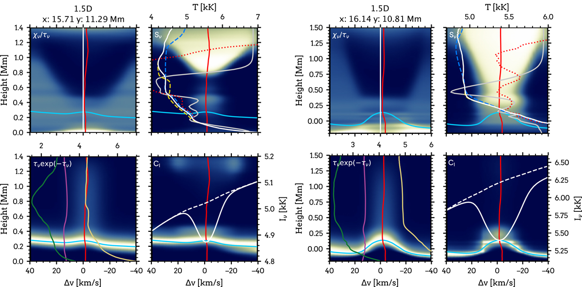
Hε four-panel diagrams for an intergranular lane (left) and a magnetic bright point (right). The locations of each point in the simulation are marked with orange and blue crosses in Fig. 10. Each diagram is organized as follows. Top left panels: relative χ_ν/τ_ν; sensitive to velocity gradients. Top right panels: S_ν: relative source function. Solid white: total source function at rest wavelength. Dashed yellow: Hε source function. Dashed blue: background source function. Source functions are displayed in brightness temperature units with the scale at the top. Solid grey: ratio of Hε to total extinction (if Hε extinction dominates the grey curve is on the left side of the plot; if Ca II H extinction dominates on the right). Dotted red: atmospheric temperature profile. Bottom-left panels: relative τ_νe^{( − τ_ν)}; indicates where most of the contribution to relative line intensity comes from. Solid green: ϵB_ν(T_e). Solid violet: σJ_ν. Solid gold: ηB_ν(T^⋆). The three terms are displayed in brightness temperature units with the scale at the top. Bottom-right panels: C_I; contribution to relative line depression. Solid white: Ca II H plus Hε line profile. Dashed white: Ca II H background line profile. Solid red: atmospheric vertical velocity profile. Solid light blue: τ = 1 height.