| Issue |
A&A
Volume 695, March 2025
|
|
|---|---|---|
| Article Number | A123 | |
| Number of page(s) | 13 | |
| Section | The Sun and the Heliosphere | |
| DOI | https://doi.org/10.1051/0004-6361/202453118 | |
| Published online | 12 March 2025 | |
Small-scale energetic phenomena in Hε: Ellerman bombs, UV bursts, and small flares
1
Rosseland Centre for Solar Physics, University of Oslo, PO Box 1029 Blindern 0315 Oslo, Norway
2
Institute of Theoretical Astrophysics, University of Oslo, PO Box 1029 Blindern, 0315 Oslo, Norway
⋆ Corresponding author; This email address is being protected from spambots. You need JavaScript enabled to view it.
Received:
21
November
2024
Accepted:
10
February
2025
Abstract
Aims. We investigated the potential of using Hε to diagnose small-scale energetic phenomena such as Ellerman bombs, UV bursts, and small-scale flares. Our focus is to understand the formation of the line and how to use its properties to get insight into the dynamics of small-scale energetic phenomena.
Methods. We carried out a forward modeling study, combining simulations and detailed radiative transfer calculations. The 3D radiative magnetohydrodynamic simulations were run with the Bifrost code and included energetic phenomena. We employed a Markovian framework to study the Hε multilevel source function, used relative contribution functions to identify its formation regions, and correlated the properties of synthetic spectra with atmospheric parameters.
Results. Ellerman bombs are predominantly optically thick in Hε, appearing as well-defined structures. UV bursts and small flares are partially optically thin and give rise to diffuse structures. The Hε line serves as a good velocity diagnostic for small-scale heating events in the lower chromosphere. However, its emission strength is a poor indicator of temperature, and its line width offers limited utility due to the interplay of various broadening mechanisms. Compared to Hα, Hε exhibits greater sensitivity to phenomena such as Ellerman bombs, as its line core experiences higher extinction than the Hα wing.
Conclusions. Hε is a valuable tool for studying small-scale energetic phenomena in the lower chromosphere. It provides more reliable estimates of velocities than those extracted from wing emission in Hα or Hβ. Maps of Hε emission show more abundant energetic events than the Hα counterpart. Our findings highlight Hε’s potential to advance our understanding of dynamic processes in the solar atmosphere.
Key words: line: formation / radiative transfer / Sun: activity / Sun: atmosphere / Sun: flares
© The Authors 2025
 Open Access article, published by EDP Sciences, under the terms of the Creative Commons Attribution License (https://creativecommons.org/licenses/by/4.0), which permits unrestricted use, distribution, and reproduction in any medium, provided the original work is properly cited.
This article is published in open access under the Subscribe to Open model. This email address is being protected from spambots. You need JavaScript enabled to view it. to support open access publication.
1. Introduction
Magnetic reconnection is widely regarded as a fundamental driver of various solar energetic phenomena, including flares, Ellerman bombs (Pariat et al. 2007; Bello González et al. 2013; Rouppe van der Voort et al. 2016), and UV bursts (Peter et al. 2014; Young et al. 2018). Flares represent the most dramatic releases of magnetic energy in the solar atmosphere, with observable signatures across spectral lines originating from the corona, chromosphere, and down to the photosphere. UV bursts (Peter et al. 2014) are chromospheric phenomena that were first observed in the Si IV lines using the Interface Region Imaging Spectrograph (IRIS; De Pontieu et al. 2014), and they are several orders of magnitude less energetic than flares. The smallest detectable transient reconnection events are commonly referred to as Ellerman bombs (Ellerman 1917; McMath et al. 1960; Severny 1956), which are observed in the solar photosphere. Ellerman bombs are traditionally detected in regions of strong magnetic activity as intense brightenings of the extended wings of the Hα line, while they remain undetectable in the Hα line core.
Rouppe van der Voort et al. (2016) show that Ellerman-bomb-like events seen in Hα are much more common than previously thought and not limited to active regions; they have even been observed in the quiet Sun, and such events have been termed quiet-Sun Ellerman bombs. Nelson et al. (2017) and Shetye et al. (2018) further explored this phenomenon. More recently, Joshi et al. (2020) and Joshi & Rouppe van der Voort (2022) revealed that quiet-Sun Ellerman bombs are more prevalent in Hβ than in Hα across the quiet Sun, which has sparked growing interest in using higher-order Balmer series lines as diagnostic tools for these small-scale energetic events.
The Balmer series line Hε is one such candidate. In the solar spectrum, this line is only a weak blend in the Ca II H wing. Its formation in the solar spectrum was first studied by Ayres & Linsky (1975), who used a 1D plane-parallel static model atmosphere. In Krikova et al. (2023, hereafter Paper I) we revisited the formation of Hε using state-of-the-art 3D radiative magnetohydrodynamic simulations (Carlsson et al. 2016) coupled with modern nonlocal thermodynamic equilibrium (non-LTE) radiative transfer codes (Uitenbroek 2001; Pereira & Uitenbroek 2015). In Paper I we find that most locations in the quiet Sun are optically thin to Hε radiation; the exceptions are regions of enhanced temperature in the lower atmosphere, where Hε extinction increases.
Earlier studies of Hε in solar energetic phenomena (e.g., Rolli & Magun 1995; Rolli et al. 1998a,b) focused on its behavior during flares. Advances in instrumentation, in particular the CHROMIS instrument (Scharmer 2006, 2007) at the Swedish 1-m Solar Telescope (SST; Scharmer et al. 2003), allow us to observe Hε at much higher spatial resolution and have re-sparked interest in this line. Rouppe van der Voort et al. (2024) made use of such novel observations to demonstrate that Hε is uniquely suited for investigations of energetic phenomena such as Ellerman bombs, even more than Hα or Hβ. Furthermore, Anan et al. (2024) emphasize that the polarization of Hε serves as a diagnostic for electric fields linked to magnetic diffusion, potentially tied to the release of magnetic energy in small-scale energetic phenomena.
Energetic events in Hε are often associated with emission, either in the line core or in the wings. The Hε emission profiles we studied in Paper I came from a relatively quiet 3D simulation, which lacked reconnection-driven large events, and therefore were associated with shocks. However, given the vast observational evidence (Rouppe van der Voort et al. 2024) that Hε emission is associated with Ellerman bombs and other events, it is worth revisiting the subject using models that actually simulate these phenomena.
In this work we investigated the fundamental formation properties of Hε in small-scale energetic phenomena, such as Ellerman bombs, UV bursts, and small-scale flares, using active simulations (Hansteen et al. 2017, 2019) run with the Bifrost code (Gudiksen et al. 2011). We sought to identify what atmospheric information can be derived from the Hε profiles for energetic events and determine where the Hε radiation originates.
We explored which transitions are responsible for the observed line photons in energetic events, encoded within the multilevel source function, using the multilevel source function description we developed in Krikova & Pereira (2024, hereafter Paper II). Finally, we aimed to quantify whether Hε is formed under optically thin or optically thick conditions during small-scale energetic events, which will provide insight into how these structures appear in observations.
The outline of the paper is as follows. Section 2 introduces the Bifrost simulations, details the calculation of synthetic spectra, and describes the methodologies used to analyze the Hε spectral profiles. In Sect. 3 we provide an overview of the synthetic spectra derived from the Bifrost simulations, determining whether the line formation is optically thick or thin. Additionally, we performed a detailed analysis of an Ellerman bomb, a UV burst, and a small-scale flare. Section 4 investigates the relationship between line parameters and atmospheric conditions, examines the broadening mechanisms affecting Hε, and compares synthetic Hα images with Hε. Our findings are discussed in Sect. 5, which is followed by concluding remarks in Sect. 6.
2. Methods
2.1. Simulations
We made use of two different 3D radiative magnetohydrodynamic simulations run with the Bifrost code (Gudiksen et al. 2011). They were solved on a Cartesian grid with 24 × 24 Mm2 in the horizontal direction and span the upper convection zone to the lower corona.
The first simulation is described by Hansteen et al. (2017), and we refer to it as the cbh simulation. It has a horizontal grid size of 48 km, and a vertical grid size of about 20 km in the photosphere and chromosphere. The simulation was evolved starting with a weak and uniform magnetic field, and then a horizontal magnetic flux sheet with 336 mT (3360 G) oriented in the y direction was injected at the bottom boundary, which later emerges to the photosphere. As they rise through the atmosphere, magnetic flux elements generate several heating events, several of which resemble Ellerman bombs and UV bursts, and even some small nano- or micro-flares (with temperatures of ≈1 MK). We used a single snapshot of this simulation, at a simulated time of 8200 s, in which several energetic events are seen.
The second simulation is described by Hansteen et al. (2019), and we refer to it as the en simulation. Its spatial resolution is slightly higher. The horizontal grid size is 31.25 km, and its vertical grid size is about 12 km in the photosphere and chromosphere. It was started from the Bifrost simulation of Carlsson et al. (2016), which has two main magnetic polarities at the surface. In a similar approach to the cbh simulation, a horizontal magnetic flux sheet with 200 mT (2000 G) oriented in the y direction was injected at the bottom boundary and allowed to evolve. On rising and interacting with the photospheric convection and upper atmospheres, the emerging magnetic flux sheet leads to several reconnection events that resemble Ellerman bombs and UV bursts. We used one snapshot, chosen at a simulation time of 9100 s, in which several energetic events are visible.
2.2. Synthetic spectra
To obtain synthetic spectra for Hε we followed the same procedure as in Paper I. The Hε spectral line is a weak blend in the wing of the much stronger Ca II H line, and therefore we needed to perform radiative transfer calculations in non-LTE (outside LTE, or local thermodynamical equilibrium) for both the hydrogen and calcium atoms.
For hydrogen, we used a model atom with eight levels plus the H II continuum and incorporated line blends in the Balmer continuum radiation. All hydrogen lines were treated using complete redistribution (CRD). We adopted the convention where the hydrogen ground level is n = 1 and the continuum is n = 9.
For calcium, we used a model atom with five levels of Ca II plus the Ca III continuum. To correctly reproduce the wing profile around Hε, we treated the Ca II H line with partial redistribution (PRD). All other lines Ca II were treated under CRD, to save computing time, since their indirect effect in the Ca II H line was negligible.
For the spectral synthesis, our main workhorse was the RH 1.5D code (Pereira & Uitenbroek 2015; Uitenbroek 2001). This code uses the 1.5D approximation, treating each simulation column as an independent 1D plane-parallel atmosphere. This is a reasonable assumption for the Hε line (see Paper I), and allows more tractable run times, since 3D non-LTE calculations with PRD are extremely expensive (Sukhorukov & Leenaarts 2017).
We wanted to also compare radiation from Hε with that from Hα, and for this line the 1.5D approximation works poorly (Leenaarts et al. 2012). We therefore also used the Multi3D code (Leenaarts et al. 2009) to obtain Hα line profiles. Here we used a simplified hydrogen model atom with a five-level plus continuum. The Ly-α and Ly-β lines were modeled under CRD, using Gaussian line profiles to approximate the effects of PRD, as described by Leenaarts et al. (2012).
Finally, we made use of the Muspel library (Pereira & Harnes 2024) to synthesize line profiles at arbitrary inclinations. Muspel includes the same continuum extinction, line profile physics, and formal solvers as RH 1.5D, and enables a flexible framework to load populations from RH 1.5D and compute radiation for different ray inclinations.
2.3. Relative contribution functions
To quantify the contribution of each layer in the simulation to the Hε line intensity, we employed relative contribution functions instead of the traditional contribution functions for intensity (Carlsson & Stein 1997). Contribution functions tell us where in the atmosphere the line is being formed. Relative contribution functions (introduced by Magain 1986, to study weak blends in strong continua) can distinguish between contributions to line emission and to line absorption. We defined the relative contribution function as
 (1)
(1)
where χνl is the line extinction, Sνl the line source function, Iνb the height-dependent background (continuum) emergent intensity, and τνR the relative optical depth. Iνb is computed by solving the radiative transfer equation using the background source function and extinction for a ray starting at the lower boundary and up to each height point. The relative optical depth can be calculated through cumulative integration of the relative extinction χνR expressed as
 (2)
(2)
where χνl refers to the line extinction, χνb to the background extinction, and Sνb to the background source function. In the case of Hε the background extinction and source function include both the Ca II H line and all continuum processes.
From Eq. (1) there are two cases when the line is absent and the relative contribution function is zero: when χνl = 0 (no absorbers), or when Sνl = Iνb. When there is a spectral line, atmospheric layers contribute to either relative line depression (Sνl < Iνb) or emission (Sνl > Iνb) We give further details on the application of relative contribution functions and Hε in Paper I. For locations with Hε emission, using either relative contribution functions or traditional contribution functions yields similar results.
2.4. Multilevel source function
To quantify the physical process contributing the most to the observed line photons, encoded in the line source function Sνl, we used the multilevel source function approach (Jefferies 1968, Canfield 1971, Rutten 2021, Paper II). The source function is divided into three different physical mechanisms responsible for adding line photons: scattering, thermal, and interlocking:
 (3)
(3)
The terms  , Bν0(Te), and Bν0(T⋆) represent the sources of photons related to the mean radiation field, the Planck function, and the interlocking source function, respectively. The coefficients σ, ϵ, and η describe which of these three physical mechanisms predominates in contributing to the line photons.
To compute the terms in Eq. (3), we used a Markovian description of the multilevel source function (Paper II). Additionally, we simplified the source function by assuming CRD and neglecting the stimulated emission term, which has a minimal effect in the shorter wavelength region of the solar spectrum. This leads to the following expression:
 (4)
(4)
where ni and gi are the populations and statistical weights of level i (u for upper level and l for lower level). Using a general solution of the statistical equilibrium equation in terms of a level-ratio solution, as expressed in Paper II, we have
 (5)
(5)
Pul and Plu are the direct transition rates (radiative and collisional) between the upper and lower levels, and vice versa. ∑u and ∑l contain the indirect transitions per second between the upper and lower levels through all intermediate levels. We replaced this population ratio in Eq. (4), obtaining
 (6)
(6)
with the indirect transition rates split into individual intermediate levels, i, with Pli and Pui representing the transition rates from the lower or upper levels to the intermediate level. The indirect transition probabilities, qil, u and qiu, l, describe the likelihood that a transition from the intermediate level i ends up in the lower or upper level, respectively. The algebraic expressions for these probabilities can be quite lengthy, but in Paper II we identify a pattern in these expressions for the indirect transition probabilities. We utilized these patterns, which resemble all nonrecurrent paths from the intermediate level i to the lower or upper level (corrected for closed loops), to identify the dominant path that determines the level ratio and thus the line source function, as given in Eq. (6).
2.5. Optical depth of Hε
We want to quantify whether the structures observed in Hε are formed under optically thin or thick conditions and follow an approach similar to that of Rathore et al. (2015), who introduce a mean formation depth τfm (Eq. 4), in terms of log10τ0 (the optical depth at the line core), to quantify the significance of optically thick or thin formation in the C II 133.4 nm and C II 133.5 nm lines.
We introduced an average formation optical depth τafd, defined as
 (7)
(7)
 (8)
(8)
where  quantifies the optical thickness or thinness at each wavelength position across the spectral profile on a logarithmic optical depth scale. The quantity τafd represents the average optical thickness or thinness of structures within a spectral line, calculated over the wavelength range bounded by λmax and λmin. The greater the deviation from zero (i.e., the more negative τafd becomes), the more optically thin structures become in a spectral line.
2.6. Line parameters and atmospheric conditions
During energetic events, Hε is often in emission. To quantify the properties of these emission profiles, we employed a composite fitting model comprising a Gaussian component and a second-degree polynomial background for the synthetic Hε profiles. Such fitting is always approximate since the line shapes vary considerably, but we find it a good approximation to extract the line shift, width, and peak intensity. The second-degree polynomial effectively accounts for the variability in the local continuum of the Ca II H wing. The resulting Hε line profile is then approximated as
 (9)
(9)
where λ0 is the fitted line shift and ΔλDfit the line width.
For optically thin lines, the Doppler width is a combination of thermal and nonthermal broadening:
 (10)
(10)
where ξ describes the nonthermal broadening. Following the approach of Rathore et al. (2015), we estimated the nonthermal broadening from the root mean square of the line of sight velocities extracted from the simulation, in the line-forming region:
 (11)
(11)
where vi is the line of sight velocity at height i, hcont is the height where the background is formed (we assumed at λ = 396.85 nm, the symmetric blue wing position of Hε at the Ca II H wing) and hrw is relative contribution function weighted average height.
Why we used hrw to estimate the nonthermal broadening and how we identified the formation region of Hε warrants further explanation. When a spectral line is optically thick, h(τλ = 1), the height where the optical depth reaches unity, is a good proxy for the height of formation. Indeed, in several forward-modeling studies, authors correlate atmospheric properties at h(τλ = 1) with parameters of spectra (e.g., Leenaarts et al. 2013; Pereira et al. 2013; Pereira & Uitenbroek 2015; Rathore et al. 2015; Leenaarts et al. 2012; Lin et al. 2017). However, when a line is formed under optically thin conditions, or if its source function varies nonlinearly over the line formation region, h(τλ = 1) is not a reliable proxy. A more accurate approach to obtaining estimates of height, temperature, velocity, or other atmospheric parameters at the region where the line forms is to weigh the quantity X by the relative contribution function (Eq. (1)):
 (12)
(12)
We used this definition to obtain not only hrw and ξ, but also temperature, line of sight velocity, and thermal broadening.
Rathore & Carlsson (2015) demonstrated that the optically thick C II 133.4 nm and C II 133.5 nm lines can be significantly affected by opacity broadening. Opacity broadening occurs when the observed spectral line width exceeds what can be explained solely by Doppler broadening (thermal and nonthermal contributions), with the excess width arising from opacity effects in an optically thick medium. To quantify opacity broadening effects in Hε, we studied how the fitted line width ΔλDfit follows the theoretical ΔλD from Eq. (10). We built ΔλD by using ξ from Eq. (11) and the thermal velocity
 (13)
(13)
where Trw is the temperature in the line-forming region following Eq. (12). Therefore, ΔλD depends only on quantities from the simulation, while ΔλDfit comes from fitting a Gaussian to the synthetic profile. In the absence of opacity broadening these should be similar, and we defined an opacity broadening factor Opf as
 (14)
(14)
If Eq. (10) holds for the synthetic profiles, we can use it to measure the nonthermal broadening from the spectra (as opposed to ξ, which is obtained from the atmospheric velocities), using vth and ΔλDfit:
 (15)
(15)
In the absence of opacity broadening, and assuming a Gaussian profile, vnth should closely follow ξ.
3. Hε in energetic events
3.1. Synthetic observables
We present an overview of the synthetic observations of Hα, Hε, and Ca II H in Fig. 1 for the en simulation, and in Fig. 2 for the cbh simulation. Both simulations contain Ellerman bombs and UV bursts, and cbh further contains two small-scale flares.
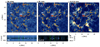 |
Fig. 1. Synthetic observables from the en simulation. The top three panels show images at the fixed wavelengths in the Hα wing, Hε core, and Ca II H core, respectively. The bottom two panels show spectrograms normalized to the continuum taken from a horizontal slice in the simulation at y ≈ 13 Mm (edges denoted by the white lines in the top panels), in Hα and Ca II H (which also includes Hε, whose location is indicated by the dashed gray line). The orange contours in the top panels indicate regions where Hε is strongly in emission, while the red contours indicate regions where Hα shows the typical signature of Ellerman bombs. The UVB and EB labels indicate the location of a UV burst and an Ellerman bomb selected for detailed study. The green vertical lines in the bottom panels indicate the approximate extent of the UV burst. |
 |
Fig. 2. Synthetic observables from the cbh simulation. The caption is the same as for Fig. 1 with the difference that the labeled events are now F1 and F2, the locations of two small flares. The vertical green lines in the bottom panels indicate the approximate position of the F1 flare. |
In the figures, we show the Hα intensity at a wing position, typically used to identify Ellerman bombs, which have a mustache-like profile with raised wings. We define regions of strong Hε emission as where the Hε core intensity exceeds 5% of its background. The background is defined as the Ca II H wing intensity at 396.85 nm, corresponding to the symmetric blue wing position of Hε. As a result, not all Ellerman bombs detected in Hα necessarily coincide with regions of strong Hε emission.
The synthetic spectra from both simulations confirm the findings of Paper I, in particular that Hε emission is an indicator of lower atmospheric heating. From Figs. 1 and 2 we see that Hε emission is more common than in the quiet-Sun simulation of Paper I and that it is often concentrated near intergranular lanes, where the magnetic field is concentrated. Hε emission is often colocated with or adjacent to Hα Ellerman bomb signatures, and regions surrounding the small flares have widespread emission in Hε. We examine a prominent Ellerman bomb, labeled in Fig. 1, in more detail in Sect. 3.2 to determine the origin of the Hε emission.
Figure 1 also demonstrates that UV bursts can produce Hε emission signatures. This is illustrated in the Ca II H plus Hε spectro-heliograms, which show multiple strong Hε emission locations throughout the UV burst structure. In Sect. 3.3 we explore the source of the Hε intensity in a UV bursts. Our synthetic profiles of Ellerman bombs and UV bursts (e.g., lower panels of Fig. 1 in between the green lines) show wing emission in Hα (with little to no signature in the core) and core emission in Hε, a signature that is consistent with observations (Rouppe van der Voort et al. 2024).
We also investigated the formation properties of Hε in small-scale flares, labeled F1 and F2 in Fig. 2. F2 is the more intense of the two. The spectrograms show a slice across F1, where both Hα and Hε are in emission at the flaring location. In Sect. 3.4 we discuss the formation mechanisms of Hε for these small-scale flare events.
To complement the spectral information, we map τafd in Fig. 3 to identify where Hε is optically thin and optically thick for both simulations. We find that Hε is optically thin in most locations in both simulations, but that regions with Hε emission tend to be optically thicker, as seen in the distributions in the lower panel of Fig. 3.
 |
Fig. 3. Average formation depth, τafd, for the Hε spectral line. Top panels:τafd maps for the en simulation (panel a) and chb simulation (panel b). The orange contours indicate regions where Hε is strongly in emission, while the red contours indicate regions where Hα shows the typical signature of Ellerman bombs. For each panel, two inserts show a zoomed-in view covering the energetic events labeled earlier: an Ellerman bomb (EB), a UV burst (UVB), and two small flares (F1 and F2). The dashed white lines in the insets indicate the horizontal slices taken for the spectrograms of Figs. 1 and 2. Panel c: Distributions of log10τafd. The emission distribution is amplified by a factor of six. |
The distribution for the en simulation peaks at log(τafd) = − 0.75, whereas the cbh distribution is skewed toward lower log(τafd) values. The light blue and red distributions indicate that Hε emission regions are optically thicker compared to their surroundings (orange and blue distributions), although a significant fraction of the locations still show optically thin structures in Hε.
To gain a more detailed perspective on the energetic events, we inserted magnified views of an Ellerman bomb, a UV burst, and small-scale flares into the corners of Fig. 3. The Hε emission associated with the Ellerman bomb structure is predominantly formed under optically thick conditions, with most of the contribution originating near the τλ = 1 layers. In locations where Hα and Hε simultaneously display Ellerman bomb signatures, it is evident that part of the Hε contribution arises from below the τλ = 1 layers. However, as we approach the western edge of the Ellerman bomb structure, the Hε-emitting regions increasingly display optically thin characteristics, with contributions coming from above the τλ = 1 layer.
The insets for more energetic events show a more dispersed distribution of optically thin and thick structures. The UV burst inset reveals that a large fraction of the Hε emission associated with the UV burst structure is formed near the τλ = 1 height, although some parts of the burst are optically thin. For the small-scale flares (F1 and F2), a significant portion of the structures seen in Hε are optically thin, indicating that layers above τλ = 1 contribute predominantly to the emergent line intensity.
3.2. Ellerman bomb
We next looked in detail at the Ellerman bomb structure labeled in Fig. 3. We aimed to determine which parts of the Ellerman bomb are observed in the Hε line and how this compares to other chromospheric lines. Additionally, we identified the transitions that govern the Hε source function within the Ellerman bomb, using Eq. (6).
In Fig. 4 we present the horizontal temperature profile of the Ellerman bomb, along with the Hε relative contribution function, to identify the layers where most line photons originate from. The relative contribution function is shown for the wavelength position where the maximum τλ = 1 height is reached within Hε. In the top panel of Fig. 4 we overplot the τλ = 1 heights for Hε with those of Ca II H, Ca II 854.2 nm, and the wing of Hα (at 656.35 nm). Ca II H and Ca II 854.2 nm probe the upper chromosphere above the Ellerman bomb structure, whereas the Ellerman bomb itself is visible in the Hα wing. Between x = 4 and x = 4.5 Mm, we observe an increase in the τλ = 1 height of the Hα wing associated with the Ellerman bomb structure.
 |
Fig. 4. Line formation through an Ellerman bomb. Panel a: Temperature slice across the atmosphere with h(τλ = 1) overplotted for the different line cores of Hε, Ca II H, and Ca II 854.2 nm and the wing of Hα at 656.35 nm. The inset shows a zoomed-in view around the Ellerman bomb, excluding h(τλ = 1) of Hε; there is a different temperature scale on top. Panel b: Relative contribution function at the maximum h(τλ = 1) over the Hε profile. |
The Hα wing captures the lower part of the Ellerman bomb, where temperatures range between 7000 and 8000 K, as shown in the inset of panel (a). The inset further reveals a temperature front, with values around 7500 K, extending and tilting upward. This temperature front is observed in Hε, as evidenced by the τλ = 1 height, which follows closely the front. This front represents the layer that predominantly contributes to the emergent line intensity, as emphasized by the relative contribution function in panel (b). Panel (b) appears largely dark over the heights where the temperature front is located because the contribution to line emission (light blue color) is precisely situated beneath the τλ = 1 line in the image. Consequently, this spatial alignment between the relative contribution function and the τλ = 1 height highlights optically thick line formation. An exception occurs at the leftmost edge of the structure (3 < x (Mm) < 3.3), where τλ = 1 is reached much lower than the region from which Hε photons originate (light blue area).
To quantify which transition pathways control the Hε source function, responsible for the majority of the emitted line photons, we present the multilevel source function in Fig. 5. It highlights why Ellerman bombs appear brighter than their surroundings. The Ellerman bomb structure shows an increase in the line source function that partly resembles the temperature structure shown in Fig. 4. In Paper II we explored the nature of indirect transition probabilities qil, u and qiu, l and provide an analytical framework to express them.
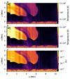 |
Fig. 5. Source function through an Ellerman bomb. Panel a: Hε source function as computed by RH 1.5D. Panel b: Approximate Hε source function from Eq. (16). Both source functions are shown on a brightness temperature scale. Panel c: Transition probability p17 from n = 1 to the upper level of Hε. |
By analyzing the transition probabilities for this event, we find that the Hε source function, as described by Eq. (6), is primarily determined by transition paths involving the ground level, denoted by P21q17, 2 and P71q12, 7. P21 is the total transition rate from the lower level of the Hε transition to n = 1, and q17, 2 the probability of reaching the upper level of the Hε transition. The total transition rate P71, combined with the probability q12, 7, describes the reverse transitions, originating from the upper level of Hε.
Looking further, we find that the dominant pathways into the transition probabilities q17, 2 and q12, 7 are the first-order paths, which connect directly the upper and lower levels of Hε with the ground level. These first-order paths are described by the probabilities p17 and p12. This means that the Hε source function can be approximated as
 (16)
(16)
In Fig. 5 we show SνRH, the line source function calculated in the RH 1.5D code, SνML (both on a brightness temperature scale), and p17 near the Ellerman bomb. We present the source functions expressed in brightness temperatures, which correspond to the temperature for which the Planck function reproduces the observed intensity to facilitate direct comparison with the atmospheric temperature. It is clear that in the Ellerman bomb region, they all show similar morphologies, strongly suggesting that the approximation in Eq. (16) is valid. The number of photons detected from the Ellerman bomb structure closely correlates with the transition probability p17.
3.3. UV burst
We depict a detailed view of line formation for a UV burst in Fig. 6. Similar to Fig. 4, it shows the temperature and Hε relative contribution function with h(τλ = 1) for different lines.
At this instant in the en simulation (t = 8200 s), the UV burst exhibits moderate temperatures above 10 000 K. In the temperature cut, it appears as a lozenge shape of enhanced temperature, at heights between 1 and 3 Mm in the chromosphere.
Hε traces the deepest layers of the UV burst, as shown by its h(τλ = 1), where it becomes optically thick to Hε radiation. This is confirmed by the overlap of the relative contribution function with h(τλ = 1). The temperatures in this Hε formation region range between 8000 and 14 000 K. The Ca II H and Ca II 854.2 nm lines are sensitive to approximately the same UV burst layers as Hε, and thus reveal comparable structures. In contrast, the Hα wing intensity is formed above Hε.
Similar to the results for the Ellerman bomb, we find that the Hε source function in the UV burst region is dominated by a first-order transition path through the ground level, as revealed by an analysis of the multilevel source function. We show this in Fig. 7, where we compare the line source function with the multilevel approximation from Eq. (16) and p17. In these panels, the UV burst structure is clearly visible in the transition probability p17, with finer structures extending from the UV burst. These finer structures, in turn, appear faintly in the temperature structure with significant contribution to relative emission, as shown in panel (b) of Fig. 6. The most distinct of these structures is located between x = 12 and x = 12.8 Mm, at an approximate height of 2 Mm, and is responsible for Hε emission that is not directly associated with the UV burst.
3.4. Small-scale flares
We next turned our attention to the small-scale flares in the cbh simulation. We focused on two events, F1 and F2. F1 is the less energetic of the two. It reaches temperatures of 10 000 K, which is not high enough to fully ionize the chromosphere. F2, on the other hand, reaches temperatures in excess of 1 MK.
We show in Fig. 8 the detailed temperature and Hε relative contribution function with h(τλ = 1) for different lines. This is similar to Figs. 4 and 6, but a difference here is that we also show h(τλ = 1) for the Hα core.
 |
Fig. 8. Line formation through two small-scale flares. The caption for each pair of panels is the same as for Fig. 4. Panels a and c are for the F1 flare, while panels b and d are for the F2 flare. In this figure there is an additional line for the h(τ) = 1 of Hα line core. |
For the F1 flare, Fig. 8 confirms that the chromosphere is not fully ionized, since h(τλ = 1) for Hα core is formed above the flare. Hε, the Hα wing, Ca II H, and Ca II 854.2 nm observe distinct parts of the event. The temperature structure of the flare is best traced at the Hα wing. Hε, Ca II H, and Ca II 854.2 nm are sensitive to the lower part of the flare’s temperature enhancement, observing similar regions. The Hε contribution to relative line emission comes from layers between 1 and 2 Mm, where temperatures reach close to 7000 K. This contribution lies slightly above h(τλ = 1), particularly at x = 13.5 Mm, indicating that parts of the flare are optically thin to Hε radiation.
The much hotter F2 flare leads to a significant degree of hydrogen ionization, which results in negligible Hα extinction and an optically thin chromosphere, as observed in Hα. Thus, both Hα and Hε observe the lower part of the flare, where temperatures remain low enough to avoid full hydrogen ionization. While Hα traces a higher layer of the flare due to its higher line extinction per particle (about 50 times that of Hε), h(τλ = 1) of Hε lies just below the region where most of the contribution to relative line emission originates, emphasizing that parts of the flare are optically thin to Hε radiation.
In Fig. 9 we examine which term in the multilevel source function (Eq. (6)) dominates the Hε source function for the hotter F2 flare. Our analysis of the multilevel source function reveals that the proportionality given in Eq. (16) holds true also for the flare structure. The transition probability p17 accurately represents the variation in the Hε source function throughout the flare, particularly in the fine structures around 2 Mm and below. These fine structures also highlight where the relative contribution to line emission originates from at x = 6.15 Mm from approximately z = 1 Mm and beyond. An increase in p17 leads to an enhanced source function and, consequently, increased Hε emission.
4. General properties of Hε in emission
4.1. Line properties
The shapes of spectral lines encode essential information about the atmospheric conditions under which the lines form. We studied the shapes of Hε profiles in the regions from both simulations where they are in emission and performed Gaussian fitting to extract three key parameters: line core intensity, width, and Doppler shift. From these, we computed additional quantities such as thermal and nonthermal broadening, and an estimate of opacity broadening (Sect. 2.6). We then compared the parameters derived from the spectra with atmospheric quantities (weighted by the relative contribution function of Hε).
We started with the line core intensity, which we show in Fig. 10. In general, the core intensity of an optically thick line is set by its source function in the line formation region. From Fig. 10, we see that indeed the Hε line core intensity exhibits a reasonable correlation with the relative contribution function weighted Hε source function, as demonstrated in panel (a). The Hε core intensity is a reliable indicator of the source function, but to which parameter is the source function related? We explore this in the other two panels of Fig. 10. A natural assumption would be temperature, displayed in panel (b). However, no significant correlation exists between temperature and the source function, except in the most optically thick regions, where the coupling to temperature is stronger. In many of the cases, the source function (and therefore line intensity) is decoupled and often below the temperature due to scattering and interlocking, similar to other chromospheric lines (e.g., Mg II h & k; see Leenaarts et al. 2013). The parameter that shows a very good correlation with the source function is the transition probability p17, shown in panel (c) (The correlation is a curved line because we are plotting the source function in a brightness temperature scale). Therefore, the Hε line core intensity serves as a proxy for the strength of the transition probability p17, which is consistent with what we found for the individual energetic events in Sects. 3.2–3.4.
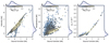 |
Fig. 10. Correlations between the properties of Hε emission profiles and atmospheric quantities. The atmospheric properties have been weighted by the relative contribution functions. Panel a: Source function and line core intensity (derived from a Gaussian fit) in brightness temperature. Panel b: Source function versus gas temperature. Panel c: Source function and transition probability p17. The color of the points indicates if Hε is optically thin or thick, as shown by the color bar that shows log10(τafd). The probability density functions of the points, calculated using Gaussian kernel density estimation, are shown at the top and right of each panel. |
Another key property of Hε is its width. The widths of Balmer lines are primarily determined by Doppler broadening or linear Stark broadening (from electrons and ions). RH 1.5D includes linear Stark broadening by electrons, following Sutton (1978), with a dependence on electron density, proportional to  . However, we find no correlation between electron density and the width of Hε (not shown in the figures), which indicates that the dominant broadening mechanisms are thermal, nonthermal, and opacity broadening.
In Fig. 11 we explore the relations between the measured Hε width, ΔλDfit, the thermal and nonthermal broadening, and the opacity broadening factor. In panel (a), we compare the thermal broadening vth, computed using the temperature weighted by the relative contribution function, with the line width. We find that the thermal broadening alone cannot explain the measured widths, which can be much larger. Most points fall to the right of the red line, which represents the width expected from thermal broadening alone. Notably, many regions with larger optical depth show widths many times larger than the thermal broadening.
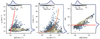 |
Fig. 11. Correlations between different contributions to the Hε broadening. Panel a: Width of Hε (ΔλDfit, from a Gaussian fit) and thermal broadening (vth). Panel b: Nonthermal broadening (vnth) and nonthermal velocity (ξ). Panel c: Width of Hε (ΔλDfit) and the opacity broadening factor (Opf). The color of the points indicates if Hε is optically thin or thick, as shown by the color bar that shows log10(τafd). The probability density functions of the points, calculated using Gaussian kernel density estimation, are shown at the top and right of each panel. The solid lines in panels a and b denote the y = x curve. |
Since thermal broadening fails to explain the observed widths, we look into how the remaining nonthermal broadening vnth from the measured widths can be explained by ξ, the nonthermal broadening estimated from velocities in the simulation. We do this in panel (b) of Fig. 11. The red line in the panel is vnth = ξ; it delineates excessive (left side) and insufficient (right side) contributions of nonthermal velocity to the line width. The values of ξ are clustered around 5 km/s, while vnth estimated from the spectral widths is typically larger. This suggests that a considerable portion of these widths cannot be explained by either thermal or nonthermal mechanisms alone. This is especially true for locations that are optically thicker, where opacity broadening is likely important.
To quantify the contribution of opacity broadening, we plot in panel (c) the opacity broadening factor (Eq. (14)) against the theoretical line width (Eq. (10)). This relation emphasizes that opacity broadening is significant, particularly for the most optically thick regions. Points above 1 (the red line) indicate cases where opacity broadening enhances the line width, while points below 1 suggest that the theoretical line width overestimates the observed width.
The next line property we looked into was the Doppler shift of Hε, which we expect can be used to diagnose velocities in the line-forming region. In Fig. 12 we plot the Doppler shift estimated from the spectra against the simulation’s line-of-sight (vertical) velocity weighted by the relative contribution function of Hε. The figure illustrates a strong correlation between atmospheric velocities and the Doppler shifts of Hε. Optically thin points (light blue) exhibit a clearer velocity-Doppler shift relationship due to their nearly ideal Gaussian profiles. In contrast, line profiles from optically thick regions often exhibit non-Gaussian shapes (e.g., central reversals), which will affect the quality of the Gaussian fit and therefore the correlation. Outliers around Doppler shifts of 50 km/s and 70 km/s likely result from profiles with central reversals, where the fitting routine misidentifies the line centroid, favoring the shorter wavelength (upflow) emission peak, creating two distinct clusters.
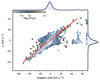 |
Fig. 12. Correlation between line-of-sight velocity, vz, and the fitted Doppler shift of the Hε line core. vz is weighted by the relative contribution function. The color of the points indicates if Hε is optically thin or thick, as shown by the color bar that shows log10(τafd). The probability density functions of the points, calculated using Gaussian kernel density estimation, are shown at the top and right. |
4.2. Hε and Hα
The spatial extent and the flame-like structure of Ellerman bombs are best observed at off-vertical inclinations (Rouppe van der Voort et al. 2016), with a μ ≡ cos θ = 0.5 being a good compromise between an inclined view but away from the limb proper, where too much superposition occurs. We generated Hα and Hε synthetic spectra for different μ using the Muspel package, using the hydrogen populations from Multi3D for Hα and RH 1.5D for Hε.
For the inclined profiles of Hε we assumed no contribution from Ca II H, only Hε. This is a strong simplification, but a good approximation for the Hε line core intensity, which is our main goal. Using results from RH 1.5D we find that neglecting Ca II H has only a minor impact on the Hε line core, and therefore use the Muspel Hε-only synthesis as a good proxy.
We show an inclined view from the simulations at μ = 0.5 in Fig. 13. The cbh simulation shows multiple brightenings in the Hα wing image, colocated with Hε line core brightenings. These brightenings are more intense in Hε, due to its higher extinction compared to the Hα wing. The higher extinction of Hε allows us to observe finer details of these structures, revealing those that could be optically thin in the Hα wing. Structures that are otherwise faint in Hα wing become prominent in Hε. This is exemplified by the flare structures F1 and F2, labeled in panel (c), where F1 appears as a tower-like structure with a blurry, veil-like appearance in Hε, but shows little to no signature in the wing of Hα. The blurry appearance of F1 in Hε results from parts of the flare being optically thin to Hε radiation, an effect even more pronounced for the more energetic flare F2.
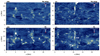 |
Fig. 13. Synthetic Hα and Hε images at an heliocentric angle of μ = 0.5. Panels a and b show an Hα wing image for the cbh and en simulations. Panels c and d show an Hε line core image for the cbh and en simulations. The wavelength position of each image is indicated by a red vertical line on top of the averaged spectral profile at the top-right corner. The Hε images are a proxy for the line core emission and were calculated by neglecting the contribution of Ca II H. |
The cbh and en simulations contain multiple Ellerman bombs, visible as flame-like structures in the Hα wing. For instance, the Ellerman bomb examined in Sect. 3.2 appears as a dome-like structure (labeled EB in panel (d)) in both Hα and Hε, although the structure is more pronounced and extended in Hε. Another notable example is the inverted Y-shaped structure, located around x ≈ 1.5 and y ≈ 16 Mm. This structure is clearly visible in the Hε line, whereas Hα only shows a faint indication of it. In general, wherever Ellerman bombs are detected in Hα, a co-spatial signature is present in Hε. However, Hε reveals more flame-like structures that are not visible in Hα. This difference comes from the larger line extinction in Hε compared to the Hα wing, which enhances the visibility of small-scale structures.
5. Discussion
We investigated the formation and observational properties of Hε for small-scale energetic events, including Ellerman bombs, UV bursts, and small-scale flares. Our focus lies on understanding how Hε behaves under varying atmospheric conditions connected to energetic events and to what degree these events can be diagnosed with Hε spectra. Ellerman bombs, UV bursts, and flares each display distinct characteristics in the Hε line. Due to high temperatures at lower column masses (chromospheric regions), UV bursts and flares appear partially optically thin in Hε, resulting in enhanced but diffuse structural features. In contrast, Ellerman bombs form in optically thick conditions with temperature increases occurring at higher column masses, which yields sharper, better-defined structures than those of UV bursts and flares.
However, it is not easy to quantify the temperature increases from Hε spectra. Its core intensity is primarily determined by the transition probability p17, and not by the temperature directly, which one might expect given that small-scale energetic events typically cause temperature enhancements. The temperature enhancements increase p17, producing more photons emitted from small-scale energetic events.
The mechanism of photon creation in Hε differs from the traditional view that the Balmer continuum primarily generates the photons for Balmer line transitions (Gebbie & Steinitz 1974; Ayres & Linsky 1975). The reason is the following. The Balmer continuum drives the radiative rates in the hydrogen atom, which leads the atomic transitions to adjust (Carlsson & Stein 2002). The changes in transition rates, particularly within the Lyman series, influence p17, which results in more photons being emitted through the ground state of hydrogen rather than through transitions into the continuum. This approach contrasts a view where the Balmer continuum is thought to ionize hydrogen, leading to recombination and cascading downward to the upper levels of the Balmer series transitions, which will eventually emit photons. However, this ionization-recombination model is unsupported by the multilevel source function, which defines the probabilities of transition paths through the atom leading to the population of the upper level of a transition eventually emitting photons (Paper II). This highlights that the emission of photons follows primarily from transitions connected to the Lyman series rather than the ionization-recombination view. They are connected to temperature in a nonlinear way, and therefore it is difficult to convert from Hε line intensity into temperature.
To date, no high-resolution observations of flares in Hε have been published. The most comprehensive results available are low-resolution observations of flares by Rolli & Magun (1995) and Rolli et al. (1998a,b), which used the Hε line width to estimate the electron density evolution in the chromosphere during flare events. These studies assumed optically thin Hε formation, no nonthermal broadening, thermal broadening at T = 104 K, and linear Stark broadening to approximate electron density. However, our analysis of the Hε widths suggests that nonthermal and opacity broadening can substantially impact the line width. They must be taken into account to obtain accurate estimates of electron density during flares. Generally, drawing definitive conclusions regarding which broadening mechanisms and atmospheric parameters primarily set the Hε width is challenging, as the full extent of the Hε profile remains “concealed” from observers. The atmosphere is optically thick to Hε wing photons, with Ca II H extinction dominating and preventing these wing photons from escaping. As a result, Hε photons can escape only near the line core, which is the visible part in observations. The more dominant Hε extinction becomes over Ca II H extinction, which is strongly temperature-dependent (due to Ly-α), the more of the Hε profile is revealed. This explains why certain data points in Fig. 11 exhibit stronger broadening than theoretical predictions (e.g., points to the left of the red line), complicating efforts to find the dominant broadening mechanism.
The Doppler shift of Hε is a good estimate of atmospheric velocities, as shown by its correlation with line-of-sight velocities. Hε can be used to measure outflows in Ellerman bombs – a measurement that is difficult to perform in Hα or Hβ. Additionally, Hε could enable detailed observations of atmospheric velocity responses to UV bursts and flares in high-resolution observations, at the atmospheric layers where the Hε line core is formed. This allows measurements of chromospheric velocities throughout the flare’s progression and across different regions of flares. The velocity estimate works better for Gaussian-shaped Hε profiles, which usually come from optically thin regions. For optically thicker regions, as seen in Fig. 12, there is more scatter in the correlation because it is difficult to reliably extract shifts from non-Gaussian profiles with central reversals and/or strong asymmetries.
Figure 13 shows more Ellerman bomb structures in Hε than in Hα. This is consistent with the observations of Rouppe van der Voort et al. (2024) and underscores the value of higher-order Balmer series lines to capture details of small-scale energetic events. For example, the Ellerman bomb structure highlighted in Fig. 13 and the inverted Y-shaped structure around x ≈ 1.5 and y ≈ 16 Mm are clearly visible in Hε but absent from Hα. These differences arise because the Hε line core has more extinction than the Hα wing, where such structures are fainter. If the extinction in small-scale energetic events is amplified due to a temperature or density increase, they can become more visible in the Hα wing. A critical assumption in synthesizing the inclined view of Hε was neglecting Ca II H, but we find it a reasonable approximation close to the line core because both the Hε extinction and source function dominate over Ca II H. As a result, our maps show granulation in the Hε core (similar to the Hα wing) instead of reversed granulation, except in regions of small-scale energetic events. The bright, diffuse structures in panel (d) reflect contributions from optically thin areas within Hε. Furthermore, we are limited by the assumption of 1.5D, but our findings in Paper I indicate that 3D effects are not pronounced for Hε.
6. Conclusions
We studied the formation of Hε in small-scale energetic phenomena from two active-Sun Bifrost simulations. We find distinct Hε signatures of Ellerman bombs, UV bursts, and flares that can offer additional diagnostics compared to other spectral lines. Key findings from our study include:
-
Flares and UV bursts exhibit partial optical thinness to Hε radiation due to strong temperature increases in the chromosphere and should appear as blurred structures in observations.
-
Ellerman bombs remain largely optically thick in Hε and appear as sharply defined structures, tracing temperature increases in the lower atmosphere.
-
Ellerman bombs are easier to see in Hε than in Hα because the line core of Hε has more extinction than the wing of Hα.
-
Hε provides good velocity diagnostics for small-scale heating events in the lower chromosphere.
-
The amount of Hε emission is a poor tracer of temperature since it is mostly set by the p17 transition probability, which depends on Lyman transitions and nonlinearly on temperature.
-
The width of Hε is poorly correlated with atmospheric properties because it is influenced by various broadening mechanisms: thermal, nonthermal, and opacity broadening.
In Paper I we demonstrate that interlocking strongly influences the line source function and, consequently, the amount of emitted Hε photons. Here, we pinpoint the p17 transition as responsible for setting Hε emission in energetic events. We show that Hε serves as a valuable diagnostic tool for detecting and analyzing small-scale energetic events, such as Ellerman bombs, UV bursts, and small-scale flares, and demonstrate how these phenomena can be observed in Hε.
Compared to other hydrogen lines, Hε is weaker but has the advantage of not being opaque enough to the fibril canopy. Therefore, it can be used to image lower chromospheric heating in its line core, not just in the wings like Hα and Hβ. This makes it more reliable for extracting velocities as the line core is easier to trace than wing emission. Its position in the Ca II H wing is both a curse and a blessing. The dominating background obscures nearly the whole Hε profile except for a small region around the core. Other lines such as Hδ and Hγ could be promising alternatives, particularly for quiet-Sun Ellerman bombs, if the chromosphere is optically thin in these lines – a possibility that merits further investigation.
Acknowledgments
This work has been supported by the Research Council of Norway through its Centers of Excellence scheme, project number 262622. Computational resources have been provided by Sigma2 – the National Infrastructure for High-Performance Computing and Data Storage in Norway. KK acknowledges support by the European Research Council under ERC Synergy grant agreement No. 810218 (Whole Sun).
References
- Anan, T., Casini, R., Uitenbroek, H., et al. 2024, Nat. Commun., 15, 8811 [NASA ADS] [CrossRef] [Google Scholar]
- Ayres, T. R., & Linsky, J. L. 1975, ApJ, 201, 212 [NASA ADS] [CrossRef] [Google Scholar]
- Bello González, N., Danilovic, S., & Kneer, F. 2013, A&A, 557, A102 [Google Scholar]
- Canfield, R. C. 1971, A&A, 10, 54 [NASA ADS] [Google Scholar]
- Carlsson, M., & Stein, R. F. 1997, ApJ, 481, 500 [Google Scholar]
- Carlsson, M., & Stein, R. F. 2002, ApJ, 572, 626 [Google Scholar]
- Carlsson, M., Hansteen, V. H., Gudiksen, B. V., Leenaarts, J., & De Pontieu, B. 2016, A&A, 585, A4 [NASA ADS] [CrossRef] [EDP Sciences] [Google Scholar]
- De Pontieu, B., Title, A. M., Lemen, J. R., et al. 2014, Sol. Phys., 289, 2733 [Google Scholar]
- Ellerman, F. 1917, ApJ, 46, 298 [NASA ADS] [CrossRef] [Google Scholar]
- Gebbie, K. B., & Steinitz, R. 1974, ApJ, 188, 399 [NASA ADS] [CrossRef] [Google Scholar]
- Gudiksen, B. V., Carlsson, M., Hansteen, V. H., et al. 2011, A&A, 531, A154 [NASA ADS] [CrossRef] [EDP Sciences] [Google Scholar]
- Hansteen, V. H., Archontis, V., Pereira, T. M. D., et al. 2017, ApJ, 839, 22 [NASA ADS] [CrossRef] [Google Scholar]
- Hansteen, V., Ortiz, A., Archontis, V., et al. 2019, A&A, 626, A33 [NASA ADS] [CrossRef] [EDP Sciences] [Google Scholar]
- Jefferies, J. T. 1968, Spectral line formation (Waltham, Mass.: Blaisdell) [Google Scholar]
- Joshi, J., & Rouppe van der Voort, L. H. M. 2022, A&A, 664, A72 [NASA ADS] [CrossRef] [EDP Sciences] [Google Scholar]
- Joshi, J., Rouppe van der Voort, L. H. M., & de la Cruz Rodríguez, J. 2020, A&A, 641, L5 [EDP Sciences] [Google Scholar]
- Krikova, K., & Pereira, T. M. D. 2024, A&A, 689, A239 [NASA ADS] [CrossRef] [EDP Sciences] [Google Scholar]
- Krikova, K., Pereira, T. M. D., & Rouppe van der Voort, L. H. M. 2023, A&A, 677, A52 [NASA ADS] [CrossRef] [EDP Sciences] [Google Scholar]
- Leenaarts, J., Carlsson, M., et al. 2009, in The Second Hinode Science Meeting: Beyond Discovery-Toward Understanding, eds. B. Lites, M. Cheung, T. Magara, et al., ASP Conf. Ser., 415, 87 [NASA ADS] [Google Scholar]
- Leenaarts, J., Carlsson, M., & Rouppe van der Voort, L. 2012, ApJ, 749, 136 [NASA ADS] [CrossRef] [Google Scholar]
- Leenaarts, J., Pereira, T. M. D., Carlsson, M., Uitenbroek, H., & De Pontieu, B. 2013, ApJ, 772, 90 [NASA ADS] [CrossRef] [Google Scholar]
- Lin, H.-H., Carlsson, M., & Leenaarts, J. 2017, ApJ, 846, 40 [NASA ADS] [CrossRef] [Google Scholar]
- Magain, P. 1986, A&A, 163, 135 [NASA ADS] [Google Scholar]
- McMath, R. R., Mohler, O. C., & Dodson, H. W. 1960, Proc. Nat. Acad. Sci., 46, 165 [NASA ADS] [CrossRef] [Google Scholar]
- Nelson, C. J., Freij, N., Reid, A., et al. 2017, ApJ, 845, 16 [Google Scholar]
- Pariat, E., Schmieder, B., Berlicki, A., et al. 2007, A&A, 473, 279 [NASA ADS] [CrossRef] [EDP Sciences] [Google Scholar]
- Pereira, T. M. D., & Harnes, E. 2024, https://doi.org/10.5281/zenodo.10854426 [Google Scholar]
- Pereira, T. M. D., & Uitenbroek, H. 2015, A&A, 574, A3 [NASA ADS] [CrossRef] [EDP Sciences] [Google Scholar]
- Pereira, T. M. D., Leenaarts, J., De Pontieu, B., Carlsson, M., & Uitenbroek, H. 2013, ApJ, 778, 143 [NASA ADS] [CrossRef] [Google Scholar]
- Peter, H., Tian, H., Curdt, W., et al. 2014, Science, 346, 1255726 [Google Scholar]
- Rathore, B., & Carlsson, M. 2015, ApJ, 811, 80 [NASA ADS] [CrossRef] [Google Scholar]
- Rathore, B., Carlsson, M., Leenaarts, J., & De Pontieu, B. 2015, ApJ, 811, 81 [NASA ADS] [CrossRef] [Google Scholar]
- Rolli, E., & Magun, A. 1995, Sol. Phys., 160, 29 [NASA ADS] [CrossRef] [Google Scholar]
- Rolli, E., Wülser, J. P., & Magun, A. 1998a, Sol. Phys., 180, 361 [NASA ADS] [CrossRef] [Google Scholar]
- Rolli, E., Wülser, J. P., & Magun, A. 1998b, Sol. Phys., 180, 343 [NASA ADS] [CrossRef] [Google Scholar]
- Rouppe van der Voort, L. H. M., Rutten, R. J., & Vissers, G. J. M. 2016, A&A, 592, A100 [NASA ADS] [CrossRef] [EDP Sciences] [Google Scholar]
- Rouppe van der Voort, L. H. M., Joshi, J., & Krikova, K. 2024, A&A, 683, A190 [NASA ADS] [CrossRef] [EDP Sciences] [Google Scholar]
- Rutten, R. J. 2021, arXiv e-prints [arXiv:2103.02369] [Google Scholar]
- Scharmer, G. B. 2006, A&A, 447, 1111 [NASA ADS] [CrossRef] [EDP Sciences] [Google Scholar]
- Scharmer, G. 2017, in SOLARNET IV: The Physics of the Sun from the Interior to the Outer Atmosphere, 85 [Google Scholar]
- Scharmer, G. B., Bjelksjo, K., Korhonen, T. K., Lindberg, B., & Petterson, B. 2003, in Innovative Telescopes and Instrumentation for Solar Astrophysics, eds. S. L. Keil, & S. V. Avakyan, SPIE Conf. Ser., 4853, 341 [NASA ADS] [CrossRef] [Google Scholar]
- Severny, A. B. 1956, The Observatory, 76, 241 [NASA ADS] [Google Scholar]
- Shetye, J., Shelyag, S., Reid, A. L., et al. 2018, MNRAS, 479, 3274 [Google Scholar]
- Sukhorukov, A. V., & Leenaarts, J. 2017, A&A, 597, A46 [NASA ADS] [CrossRef] [EDP Sciences] [Google Scholar]
- Sutton, K. 1978, J. Quant. Spectr. Rad. Transf., 20, 333 [NASA ADS] [CrossRef] [Google Scholar]
- Uitenbroek, H. 2001, ApJ, 557, 389 [Google Scholar]
- Young, P. R., Tian, H., Peter, H., et al. 2018, Space Sci. Rev., 214, 120 [Google Scholar]
All Figures
|
Fig. 1. Synthetic observables from the en simulation. The top three panels show images at the fixed wavelengths in the Hα wing, Hε core, and Ca II H core, respectively. The bottom two panels show spectrograms normalized to the continuum taken from a horizontal slice in the simulation at y ≈ 13 Mm (edges denoted by the white lines in the top panels), in Hα and Ca II H (which also includes Hε, whose location is indicated by the dashed gray line). The orange contours in the top panels indicate regions where Hε is strongly in emission, while the red contours indicate regions where Hα shows the typical signature of Ellerman bombs. The UVB and EB labels indicate the location of a UV burst and an Ellerman bomb selected for detailed study. The green vertical lines in the bottom panels indicate the approximate extent of the UV burst. |
| In the text | |
|
Fig. 2. Synthetic observables from the cbh simulation. The caption is the same as for Fig. 1 with the difference that the labeled events are now F1 and F2, the locations of two small flares. The vertical green lines in the bottom panels indicate the approximate position of the F1 flare. |
| In the text | |
|
Fig. 3. Average formation depth, τafd, for the Hε spectral line. Top panels:τafd maps for the en simulation (panel a) and chb simulation (panel b). The orange contours indicate regions where Hε is strongly in emission, while the red contours indicate regions where Hα shows the typical signature of Ellerman bombs. For each panel, two inserts show a zoomed-in view covering the energetic events labeled earlier: an Ellerman bomb (EB), a UV burst (UVB), and two small flares (F1 and F2). The dashed white lines in the insets indicate the horizontal slices taken for the spectrograms of Figs. 1 and 2. Panel c: Distributions of log10τafd. The emission distribution is amplified by a factor of six. |
| In the text | |
|
Fig. 4. Line formation through an Ellerman bomb. Panel a: Temperature slice across the atmosphere with h(τλ = 1) overplotted for the different line cores of Hε, Ca II H, and Ca II 854.2 nm and the wing of Hα at 656.35 nm. The inset shows a zoomed-in view around the Ellerman bomb, excluding h(τλ = 1) of Hε; there is a different temperature scale on top. Panel b: Relative contribution function at the maximum h(τλ = 1) over the Hε profile. |
| In the text | |
|
Fig. 5. Source function through an Ellerman bomb. Panel a: Hε source function as computed by RH 1.5D. Panel b: Approximate Hε source function from Eq. (16). Both source functions are shown on a brightness temperature scale. Panel c: Transition probability p17 from n = 1 to the upper level of Hε. |
| In the text | |
 |
Fig. 6. Line formation through a UV burst. The caption is the same as for Fig. 4. |
| In the text | |
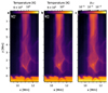 |
Fig. 7. Source function through a UV burst. The caption is the same as for Fig. 5. |
| In the text | |
|
Fig. 8. Line formation through two small-scale flares. The caption for each pair of panels is the same as for Fig. 4. Panels a and c are for the F1 flare, while panels b and d are for the F2 flare. In this figure there is an additional line for the h(τ) = 1 of Hα line core. |
| In the text | |
 |
Fig. 9. Source function through small-scale flare F2. The caption is the same as for Fig. 5. |
| In the text | |
|
Fig. 10. Correlations between the properties of Hε emission profiles and atmospheric quantities. The atmospheric properties have been weighted by the relative contribution functions. Panel a: Source function and line core intensity (derived from a Gaussian fit) in brightness temperature. Panel b: Source function versus gas temperature. Panel c: Source function and transition probability p17. The color of the points indicates if Hε is optically thin or thick, as shown by the color bar that shows log10(τafd). The probability density functions of the points, calculated using Gaussian kernel density estimation, are shown at the top and right of each panel. |
| In the text | |
|
Fig. 11. Correlations between different contributions to the Hε broadening. Panel a: Width of Hε (ΔλDfit, from a Gaussian fit) and thermal broadening (vth). Panel b: Nonthermal broadening (vnth) and nonthermal velocity (ξ). Panel c: Width of Hε (ΔλDfit) and the opacity broadening factor (Opf). The color of the points indicates if Hε is optically thin or thick, as shown by the color bar that shows log10(τafd). The probability density functions of the points, calculated using Gaussian kernel density estimation, are shown at the top and right of each panel. The solid lines in panels a and b denote the y = x curve. |
| In the text | |
|
Fig. 12. Correlation between line-of-sight velocity, vz, and the fitted Doppler shift of the Hε line core. vz is weighted by the relative contribution function. The color of the points indicates if Hε is optically thin or thick, as shown by the color bar that shows log10(τafd). The probability density functions of the points, calculated using Gaussian kernel density estimation, are shown at the top and right. |
| In the text | |
|
Fig. 13. Synthetic Hα and Hε images at an heliocentric angle of μ = 0.5. Panels a and b show an Hα wing image for the cbh and en simulations. Panels c and d show an Hε line core image for the cbh and en simulations. The wavelength position of each image is indicated by a red vertical line on top of the averaged spectral profile at the top-right corner. The Hε images are a proxy for the line core emission and were calculated by neglecting the contribution of Ca II H. |
| In the text | |
Current usage metrics show cumulative count of Article Views (full-text article views including HTML views, PDF and ePub downloads, according to the available data) and Abstracts Views on Vision4Press platform.
Data correspond to usage on the plateform after 2015. The current usage metrics is available 48-96 hours after online publication and is updated daily on week days.
Initial download of the metrics may take a while.