| Issue |
A&A
Volume 686, June 2024
|
|
|---|---|---|
| Article Number | A218 | |
| Number of page(s) | 10 | |
| Section | The Sun and the Heliosphere | |
| DOI | https://doi.org/10.1051/0004-6361/202348894 | |
| Published online | 13 June 2024 | |
Small-scale magnetic flux emergence preceding a chain of energetic solar atmospheric events⋆
1
Instituto de Astrofísica de Canarias, 38205 La Laguna, Tenerife, Spain
e-mail: This email address is being protected from spambots. You need JavaScript enabled to view it.
2
Universidad de La Laguna, Dept. Astrofísica, 38206 La Laguna, Tenerife, Spain
3
Rosseland Centre for Solar Physics, University of Oslo, PO Box 1029 Blindern, 0315 Oslo, Norway
4
Institute of Theoretical Astrophysics, University of Oslo, PO Box 1029 Blindern, 0315 Oslo, Norway
5
Universidad de La Laguna, Dept. Didácticas Específicas, 38200 La Laguna, Tenerife, Spain
6
Lockheed Martin Solar and Astrophysics Laboratory, Palo Alto, CA 94304, USA
7
Bay Area Environmental Research Institute, NASA Research Park, Moffett Field, CA 94035, USA
8
LPC2E, CNRS/CNES/University of Orléans, 3A Avenue de la Recherche Scientifique, Orléans, France
Received:
9
December
2023
Accepted:
17
March
2024
Abstract
Context. Advancements in instrumentation have revealed a multitude of small-scale extreme-ultraviolet (EUV) events in the solar atmosphere and considerable effort is currently undergoing to unravel them.
Aims. Our aim is to employ high-resolution and high-sensitivity magnetograms to gain a detailed understanding of the magnetic origin of such phenomena.
Methods. We used coordinated observations from the Swedish 1-m Solar Telescope (SST), the Interface Region Imaging Spectrograph (IRIS), and the Solar Dynamics Observatory (SDO) to analyze an ephemeral magnetic flux emergence episode and the following chain of small-scale energetic events. These unique observations clearly link these phenomena together.
Results. The high-resolution (0.″057 pixel−1) magnetograms obtained with SST/CRISP allowed us to reliably measure the magnetic field at the photosphere and to detect the emerging bipole that caused the subsequent eruptive atmospheric events. Notably, this small-scale emergence episode remains indiscernible in the lower resolution SDO/HMI magnetograms (0.″5 pixel−1). We report the appearance of a dark bubble in Ca II K 3933 Å related to the emerging bipole, a sign of the canonical expanding magnetic dome predicted in flux emergence simulations. Evidence of reconnection are also found, first through an Ellerman bomb and later by the launch of a surge next to a UV burst. The UV burst exhibits a weak EUV counterpart in the coronal SDO/AIA channels. By calculating the differential emission measure (DEM), its plasma is shown to reach a temperature beyond 1 MK and to have densities between the upper chromosphere and transition region.
Conclusions. Our study showcases the importance of high-resolution magnetograms in revealing the mechanisms that trigger phenomena such as EBs, UV bursts, and surges. This could hold implications for small-scale events similar to those recently reported in the EUV using Solar Orbiter. The finding of temperatures beyond 1 MK in the UV burst plasma strongly suggests that we are examining analogous features. Therefore, we recommend caution when drawing conclusions from full-disk magnetograms that lack the necessary resolution to reveal their true magnetic origin.
Key words: methods: observational / Sun: chromosphere / Sun: corona / Sun: photosphere / Sun: transition region
Movies are available at https://www.aanda.org
© The Authors 2024
 Open Access article, published by EDP Sciences, under the terms of the Creative Commons Attribution License (https://creativecommons.org/licenses/by/4.0), which permits unrestricted use, distribution, and reproduction in any medium, provided the original work is properly cited.
This article is published in open access under the Subscribe to Open model. This email address is being protected from spambots. You need JavaScript enabled to view it. to support open access publication.
1. Introduction
The emergence of magnetic flux from the solar interior into the photosphere and upper layers triggers a wide variety of eruptive and ejective phenomena in the solar atmosphere. From observations, there are several reports about the subsequent phenomena following magnetic flux emergence:
-
Ellerman bombs (EBs, e.g., Pariat et al. 2004; Hashimoto et al. 2010; Watanabe et al. 2011; Nelson et al. 2013; Rutten et al. 2013; Vissers et al. 2013; Reid et al. 2016; Yang et al. 2016; Rouppe van der Voort et al. 2021, 2023; Shen et al. 2022);
-
surges (e.g., Liu & Kurokawa 2004; Guglielmino et al. 2010, 2019; Vargas Domínguez et al. 2014; Kim et al. 2015; Nóbrega-Siverio et al. 2017; Verma et al. 2020; Díaz Baso et al. 2021; Nóbrega-Siverio et al. 2021);
-
ultraviolet (UV) bursts (e.g., Peter et al. 2014; Vissers et al. 2015; Grubecka et al. 2016; Rouppe van der Voort et al. 2017; Young et al. 2018; Tian et al. 2018; Guglielmino et al. 2018; Chen et al. 2019; Ortiz et al. 2020);
-
coronal jets (e.g., Shibata et al. 1992; Canfield et al. 1996; Liu et al. 2011; Huang et al. 2012; Schmieder et al. 2013; Ruan et al. 2019; Joshi et al. 2020a).
Recently, improvements in observational capabilities, such as the Extreme Ultraviolet Imager of the High Resolution Imager (EUI-HRI; Rochus et al. 2020) on board Solar Orbiter (SolO; Müller et al. 2020), have revealed a forest of small-scale events visible in the corona. This includes a phenomenon called campfires (e.g., Berghmans et al. 2021; Zhukov et al. 2021; Kahil et al. 2022; Dolliou et al. 2023; Huang et al. 2023), which are small-scale EUV brightenings in the quiet Sun, and small inverted Y-shaped jets with a base width down to ≤1 Mm (Mandal et al. 2022; Chitta et al. 2023; Panesar et al. 2023). In order to broaden our comprehension of their origins, it is crucial to understand the connection to the topology and evolution of the magnetic field. This requires coordination of the coronal observations with observations at other wavelengths and spectropolarimetry to cover the full solar atmosphere. High sensitivity in magnetograms is essential for revealing the appearance of emerging small-scale magnetic loops and accurately characterizing the magnetic flux. For example, Guglielmino et al. (2018) found that the magnetic flux measured in an emerging region with the Helioseismic and Magnetic Imager (HMI; Scherrer et al. 2012) on board the Solar Dynamics Observatory (SDO; Pesnell et al. 2012) is three times smaller than the flux measured with the higher resolution Solar Optical Telescope (SOT; Tsuneta et al. 2008) on board Hinode (Kosugi et al. 2007). Furthermore, high spatial resolution, in observations that sample the lower atmosphere, is important to be able to detect the rise of the small-scale loops through the atmosphere and their interaction with the pre-existing ambient field. For instance, using HINODE/SOT, Vargas Domínguez et al. (2012) and Kontogiannis et al. (2020) identified, in Ca II H images, elliptical dark features with a lifetime of ≈12 min located between the footpoints of emerging bipoles, a finding also reported by Centeno et al. (2017) through Ca II H observations with SUNRISE II (Solanki et al. 2017). Similar features visible in Ca II 8542 Å were described by Ortiz et al. (2014, 2016), de la Cruz Rodríguez et al. (2015b), using the Swedish 1-m Solar Telescope (SST; Scharmer et al. 2003). Further evidence using other spectral lines is necessary to better constrain the magnetic flux emergence through the lower atmosphere.
In this work we present a small-scale magnetic flux emergence episode observed on 2017 May 25 using SST, the Interface Region Imaging Spectrograph (IRIS; De Pontieu et al. 2014), and SDO, underscoring the absolute necessity of sensitive magnetograms for detecting such events. The episode exhibited a wide variety of signatures in all the atmospheric layers resulting from magnetic flux emergence and subsequent reconnection with the pre-existing ambient field. The layout of this paper is as follows. In Sect. 2 we describe the coordinated observations and the alignment between them. In Sect. 3 we show the results and analyze the magnetic flux emergence episode through different resolution magnetograms (Sect. 3.1). We later describe all the phenomena related to it, namely the dark bubble (Sect. 3.2), the Ellerman bomb (Sect. 3.3), as well as UV burst and surge along with their EUV counterparts (Sects. 3.4 and 3.5). Finally, Sect. 4 contains the discussion and the main conclusions.
2. Observations
We used coordinated observations from SST, IRIS, and SDO obtained on 2017 May 25 from 08:07:54 to 09:02:42 UT of an enhanced network region near disk center at heliocentric coordinates (x, y) = (36″, −91″) and observing angle μ = 0.99. This dataset was acquired as part of a multi-season effort to acquire coordinated observations of different targets with SST and IRIS (see Rouppe van der Voort et al. 2020). The observations are unique, with a combination of precise co-pointing and excellent seeing conditions over an extended period. All instruments delivered consistent high-quality data to cover the full evolution of the sequence of events.
The SST dataset contains the following spectral scans obtained with the CRisp Imaging Spectropolarimeter (CRISP; Scharmer et al. 2008): the Fe I 6301 and 6302 Å line pair in spectropolarimetric mode and Hα 6563 Å in spectroscopic mode. The Fe I 6301 and 6302 Å lines were sampled in 16 positions between −1178 mÅ and +90 mÅ from the 6302 Å line core. For each line position and polarization state, six exposures were acquired that were used for image restoration (i.e., a total of 384 exposures per spectral line scan). The noise level in the restored Stokes V/Icont maps was estimated to be 2 × 10⁻³. The Hα line was sampled in 32 positions ranging from −1850 mÅ to +1850 mÅ from the line core. The CRISP scans have a temporal cadence of 19.5 s, a spatial sampling of 0.″057 per pixel, and a field of view (FOV) of ∼58″ × 58″.
In addition, the SST dataset contains spectral scans from the CHROmospheric Imaging Spectrometer (CHROMIS) for the Ca II K 3934 Å line, which is sampled in 41 positions between −1300 mÅ and +1300 mÅ from the line core. In addition, one continuum wavelength at 4000 Å was recorded. The CHROMIS scans have a temporal cadence of 13.8 s, a spatial sampling of 0.″038 per pixel, and a FOV of 66″ × 42″.
The CRISP and CHROMIS data were processed using the SSTRED data reduction pipeline (de la Cruz Rodríguez et al. 2015a; Löfdahl et al. 2021), which includes Multi-Object Multi-Frame Blind Deconvolution (MOMFBD; Van Noort et al. 2005) image restoration and the method for intra-scan consistency of Henriques (2012). High image quality was achieved via the combination of the SST adaptive optics system (Scharmer et al. 2024), MOMFBD image restoration, and excellent seeing conditions. The CRISP and CHROMIS time series were coaligned such that the CRISP data matched the CHROMIS pixel scale and the CHROMIS data matched the CRISP temporal cadence. More details about the observing program and data processing are provided by Bose et al. (2021), who analyzed a 97 min time series of the same target that started shortly after the dataset we present here.
Line-of-sight (LOS) magnetograms were obtained by performing Milne-Eddington inversions of the Fe I 6301 and 6302 Å Stokes profiles following the scheme developed by de la Cruz Rodríguez (2019)1. By measuring the standard deviation in a very quiet region, we estimated the noise level in the BLOS maps to be 7 G.
The IRIS dataset was acquired with the observation program OBSID 3633105426. The spectral information was acquired through medium dense raster scans, with the spectrograph slit covering 62″ in the y direction and scanning 2″ in the x direction in eight steps of 0.″35, with an exposure time of 2 s and a raster cadence of 25 s. The slit-jaw images (SJI) covered a FOV of 60″ × 68″ with a cadence of 6 s, obtaining a total of 4000 images in the 1400 Å and 2796 Å passbands. The IRIS data were co-aligned to SST by cross-correlation between Ca II K and SJI 2796 Å, similarly to Bose et al. (2019). We estimated that the alignment precision is better than the size of the IRIS pixel (0.″17, see Rouppe van der Voort et al. 2020). We have also employed data from HMI and the Atmospheric Imaging Assembly (AIA; Lemen et al. 2012) on board SDO. The precision error for 45-s BLOS maps is around 10 G (Liu et al. 2012, also see the HMI data documentation2). Regarding the alignment, we used the routines developed by Prof. Rob Rutten and detailed documented in his manual3. A first cross-alignment was performed in all the AIA channels to the HMI continuum. Then, HMI continuum images are co-aligned to Ca II K wideband channels. The resulting EUV cross-alignments usually reach a 0.″1 precision.
Figure 1 and the associated animation illustrate the observations on 2017 May 25 analyzed in this paper. The first row displays the extended context of the observations. The region of interest is highlighted with a green square and is shown in detail in the bottom two rows. Panels (e) and (f) contain LOS magnetograms indicating the location of the emerged bipole that leads to the chain of energetic solar atmospheric events. In panels (g) and (h), the surge is identifiable as an elongated and dark structure in Hα and Ca II K, respectively. Panel (i) shows IRIS/SJI 1400 Å with a UV burst: the compact area with enhanced emission in the middle of the panel around (10″, 12″). Panels (j), (k), and (l) show the counterparts of the UV burst and surge in coronal SDO/AIA channels, the former as a weak brightening co-located with the UV burst, and the latter as a dark absorption feature in AIA at the same position of the surge.
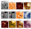 |
Fig. 1. Coordinated observations on 2017 May 25 at ∼08:48 UT. Panel (a): LOS magnetogram for SST/CRISP. Panel (b): Hα at −32 km s−1 from SST/CRISP. Panel (c): IRIS/SJI 1400 Å aligned to SST. Panel (d): SDO/AIA 193 Å aligned to SST. The 19″ × 19″ field of view highlighted in green encompasses the region of interest shown in the rest of the panels. Panels (e) and (f): LOS magnetograms for SST/CRISP and SDO/HMI aligned to SST, respectively. The red rectangle delimits the area where magnetic flux is analyzed in Sect. 3.1. Panel (g): Hα at −32 km s−1 from SST/CRISP. The colored diamonds indicate the location of the spectral profiles shown in Sect. 3.5. Panel (h): Ca II K at 10 km s−1 taken with SST/CHROMIS. Panel (i): IRIS/SJI 1400 Å with eight lines indicating the approximate locations of the spectrograph slit and the area covered by the raster scan. The light curves within the light gray rectangle are studied in Sect. 3.4. Panels (j), (k), and (l): SDO/AIA 171 Å, 193 Å, and 211 Å, respectively. In all the zoomed-in panels, the colored contours delimit the surge in the Hα blue wing (blue) and the UV burst on the IRIS/SJI 1400 (green). An animation of this figure is available online with the evolution of the system from 08:15 to 09:02 UT. |
3. Results
3.1. The magnetic flux emergence episode
We begin the analysis of the magnetic flux emergence episode by comparing panels (a) and (b) of Fig. 2, which show a close-up of the SST/CRISP and the aligned SDO/HMI magnetograms, respectively. In the figure, a clear bipole is discernible in the high-resolution (0.″057 pixel−1) SST/CRISP magnetograms. The bipole appears around 08:17 UT (see associated animation) and rapidly shows diverging opposite polarities reaching a maximum separation around 3″. The bipole is discernible for approximately 20 min, until its negative polarity merges with the preexisting surrounding negative field and the positive polarity starts to collide against the negative environment. In contrast, the lower resolution SDO/HMI magnetograms (0.″5 pixel−1) can only detect a slight increase in the positive magnetic field across a few pixels. This makes it challenging to relate it to a clear emerging bipole. This result is not altered by the interpolations from the rotation and alignment of the SDO/HMI data to SST/CRISP, as demonstrated in panel (c) of Fig. 2, with the original magnetogram from HMI. We further inspected the capabilities of SDO/HMI applying deconvolution following the method of Norton et al. (2018), which enhances the SDO/HMI signal by correcting it from scattered light. The result is shown in panel (d) labeled as SDO/HMI deconvolved. In this case the positive magnetic field exhibits higher contrast, but a discernible emerging bipole remains elusive.
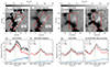 |
Fig. 2. Magnetic flux emergence episode. Panels (a) and (b): LOS magnetograms, respectively, from SST/CRISP and SDO/HMI aligned to SST. Panels (c) and (d): LOS magnetograms from the original SDO/HMI data without and with deconvolution, respectively. Panels (e), (f), (g), and (h): Magnetic flux evolution within the red rectangle for the corresponding magnetograms, showing the unsigned flux (black), the positive flux (blue), and the absolute value of the negative flux (red). In panels (e) and (g), the gray band represents the standard deviation of the unsigned flux measured in the original SST/CRISP and SDO/HMI data, respectively. An animation of this figure is available online showing the time evolution from 08:07 to 08:59 UT. |
We delved into the characterization of this event by measuring the magnetic flux within the red rectangle depicted in the respective magnetograms. The measurements for the unsigned flux (black), positive flux (blue), and absolute value of the negative flux (red) are shown in the bottom row of Fig. 2. In panel (e) the unsigned magnetic flux measured with SST/CRISP is plotted with its standard deviation (gray band). The values obtained ([0.6 − 1.1]×1019 Mx) are within the ephemeral flux region category (Zwaan 1987) and fit with the flux values reported in other similar emergence episodes (see, e.g., Guglielmino et al. 2010; Joshi et al. 2017). The positive flux shows a linear increase from 08:17 UT onward as the bipole emerges. On the contrary, the homologous measurement from the aligned SDO/HMI (panel f) does not capture that trend and underestimates the positive flux up to a factor ≈4. For the negative flux, the underestimation can be up to 1.3 at the peak of the event at 08:31 UT. This difference is independent of the rotation and alignment of the SDO/HMI data. We demonstrate that by measuring the flux in the original data (panel g), and obtained the same result. If we consider the 10 G precision error specified by the HMI team for the unsigned flux in the original SDO/HMI data (gray band), we cannot still reproduce the flux measured using SST/CRISP. The discrepancy in the magnetic flux is noticeably reduced when measuring it in the SDO/HMI deconvolved data (panel h), although it still underestimates the flux of the event.
In addition to the described bipolar emergence episode, other secondary smaller bipoles are emerging around the main event. For instance, SST/CRISP magnetograms show a tiny bipole emerging around 08:49 UT centered at (7.″0, 10.″5) which roughly lasts for five minutes (see associated animation). Instead, SDO/HMI does not show any hint of the existence of this event. Its resolution is not high enough to resolve this tiny bipole whose size is around 1″. The appearance of tiny bipoles around a main dominant one in ephemeral flux regions can also be found in numerical experiments (Nóbrega-Siverio et al. 2016).
3.2. The dark bubble
The effects of magnetic flux emergence become immediately apparent in the lower atmosphere as illustrated in Fig. 3. Panel (a) shows the SST/CRISP magnetogram, providing context, while panel (b), shows a Ca II K map in the blue wing at −49 km s−1. The latter displays a roundish dark structure, or bubble, situated between the bipole polarities. In the animation, the dark bubble becomes perceptible around 08:21 UT, four minutes after the emergence appears in the photosphere. Subsequently, the bubble expands in alignment with the diverging motion of the bipole polarities, reaching a maximum size of 3″ and lasting for 18 min. The spectral profile at approximately the center of the bubble is shown as a solid orange curve in panel (c), alongside the average Ca II K profile of the observation (orange dashed curve). Within the dark bubble, the Ca II K wings exhibit noticeable faintness, about 1.5 times weaker than the average profile, suggesting a temperature decrease in the lower atmosphere, specifically, a few hundred kilometers above the surface.
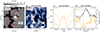 |
Fig. 3. Dark bubble. Panel (a): LOS magnetogram from SST/CRISP. Panel (b): Ca II K map at −49 km s−1 from SST/CHROMIS. Panel (c): Ca II K profiles normalized to the continuum for the location marked in panel (b) (solid line), and the average over the whole FOV of the observation (dashed line). Panel (d): Time evolution of the normalized Ca II K intensity at −49 km s−1 for the position indicated in panel (b) (orange), and the unsigned magnetic flux from SST/CRISP within the red rectangle (black). An animation of this figure is available online showing the time evolution from 08:07 to 08:59 UT. |
The relationship between the emergence episode and the appearance of this dark bubble is also evident in panel (d), which demonstrates how the intensity of Ca II K at −49 km s−1 at the center of the bubble diminishes while the magnetic flux increases; in other words, they are anti-correlated. Thus, the appearance of dark bubbles may serve as additional indirect indicators of magnetic flux emergence when high-resolution magnetograms are not available. The secondary tiny bipole described in the previous section also exhibits an associated dark bubble at approximately 08:49 UT centered at (7.″0, 10.″5) (see associated animation).
We checked the IRIS/SJI 2796 Å images to see if we could discern a similar dark pattern associated with the bubble similar to the one reported by Ortiz et al. (2016); nonetheless, we were not able to distinguish any clear high-contrast dark feature. We also examined the IRIS Mg II h&k spectra; however, the overlap of the IRIS slit with the bubble is not perfect, so the results are inconclusive.
3.3. The Ellerman bomb
Once the emerging magnetized plasma reaches the lower atmosphere, it interacts with the pre-existing magnetic field, giving rise to an EB. As an illustration, panels (a) and (e) of Fig. 4 contain far-blue wing maps of the Hα and Ca II K lines, respectively. The EB manifests as an enhanced, blob-like brightening in both maps, as indicated by the arrows. In the associated animation, we can distinguish its appearance at around 08:28 UT, which is seven minutes after the initial indications of the dark bubble. Following the motion of the EB, we can estimate its lifetime to be around 7 min. During this time, the EB exhibits rapid changes in its apparent shape and size, covering an area up to approximately 0.6 arcsec2, which is within the typical values reported in the literature (see, e.g., Vissers et al. 2013). The EB’s location, at (9.″8, 11.″8), coincides with the region where the positive polarity of the emerging bipole encounters a pre-existing negative concentration: a favorable configuration for magnetic reconnection. Panels (b) and (f) display the λ − t plot at that particular location for Hα and Ca II K, respectively. Furthermore, panels (c) and (g) show the comparison between the EB profile (solid) and the average profile over the whole FOV of the observation (dashed) for both spectral lines. In these panels the enhancement in the wings of the Hα and Ca II K lines is clearly visible, which is a defining feature of EBs (see, e.g., Rouppe van der Voort et al. 2017; Leenaarts et al. 2018; Vissers et al. 2019a, among others cited in the Introduction), corroborating the magnetic reconnection scenario. Additional indications of the EB can be observed in the SDO/AIA 1600 and 1700 Å channels (panels d and h) through a co-spatial slight intensity increase (see associated animation). This agrees with previous observational results (see Vissers et al. 2019a, and references therein) and further supports the validity of the automated procedure for identifying EBs using SDO data by Vissers et al. (2019b).
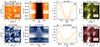 |
Fig. 4. Ellerman Bomb. Panels (a) and (e): Maps of the Hα and Ca II K lines, respectively, in the far-blue wing. The location of the EB centered at (9.″8, 11.″8) is indicated with a circle. Panels (b) and (f): λ − t plot at the center of the EB for Hα and Ca II K, respectively. The vertical red line indicates the spectral position shown in panels (a) and (e), while the horizontal green line indicates the time. Panels (c) and (g): Comparison between the spectral profile of the EB (solid) and the average profile over the whole FOV of the observation (dashed) for Hα and Ca II K, respectively. Panels (d) and (h): SDO/AIA 1600 and 1700 Å channels aligned to SST. An animation of this figure is available online showing the time evolution from 08:25 to 08:35 UT. |
3.4. The UV burst
Additional evidence of magnetic reconnection is found following the EB by the appearance of a UV burst at 08:41 UT in the IRIS SJI/1400 Å channel (see Fig. 1 and the accompanying animation). During its lifetime, the UV burst extends up to a width of ∼2″ and a length of ∼3″. We calculated the total intensity I within the light gray rectangle depicted in Fig. 1 and standardized it; that is, we subtracted the average Imean and divided it by the standard deviation Istd. The result is presented in Fig. 5 as a black line. The UV burst experiences a rapid increase in intensity over four minutes until it reaches its maximum at 08:45 UT. Subsequently, the intensity follows a gradual decline, punctuated by sporadic and sudden bursts of intensity enhancements, until it disappears around 09:00 UT, resulting in a UV burst lifetime of 19 min. This bursty behavior is one of the most characteristic identifying features of UV bursts (Young et al. 2018). Interestingly, the UV burst also exhibits a weak EUV counterpart during its lifetime. This is more evident in the intensity curves of various SDO/AIA channels depicted as colored lines in Fig. 5. In the plot, the SDO/AIA 94 Å (green), 193 Å (red), and 211 Å (blue) curves increase immediately after the maximum of the UV burst, peaking around 08:47:12 UT, whereas the SDO/AIA 171 Å channel (yellow) shows a bursty behavior with multiple peaks, more similar to the behavior detected in UV, reaching its maximum intensity slightly later.
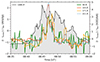 |
Fig. 5. Standardized intensity calculated within the light gray rectangle shown in Fig. 1. The curve from IRIS (left axis) shows the UV burst in SJI 1400 Å (black), whereas the curves from SDO (right axis) depict its EUV counterpart in the AIA filters 94 Å (green), 193 Å (red), 171 Å (yellow), and 211 Å (blue). |
To determine whether the SDO/AIA response signifies a bright transition region (see, e.g., Viall & Klimchuk 2015) or whether it reflects a genuine MK response, we used the approach developed by Plowman & Caspi (2020) to calculate the differential emission measure (DEM) on the original SDO/AIA data. This code solves for the undetermined DEM inversion problem by employing the Tikhonov regularization technique (more commonly known as the L2 norm). The idea behind this technique is to impose an additional mathematical constraint in the merit function (see Eq. (14) of Plowman & Caspi 2020) that helps to converge the inversion and discards any physical meaningless solutions. In return, the algorithm guarantees positive DEM solutions. Panels (a)–(d) of Fig. 6 contain 2D maps centered on the UV burst showing the emission measure (EM) integrated in bins of log10(T[K]) = 0.1 and covering a temperature range of log10(T[K]) = [6.0, 6.4]. This analysis indicates that the increase in the SDO/AIA light curves we could see in Fig. 5 around 08:47:12 UT corresponds to an enhancement of the emission at temperatures greater than log10(T[K]) = 6.1, which supports the idea that the plasma in the burst is heated above MK temperatures. To delve into this, we calculated the total EM of the area around the UV burst and a quiet reference area, including the error on the recovered EM. The error is calculated through a Monte Carlo approach (Press et al. 1992) with 100 random realizations of the input AIA data within the noise range. The EM is then computed for all the different realizations, which provides a measure of the errors through the standard deviation of the obtained solutions. This is a common approach, as implemented in the DEM code by Hannah & Kontar (2012), and it has been widely adopted for studying inversions from AIA observations (see, e.g., Su et al. 2018; Devi et al. 2022). For a comprehensive overview of errors, we refer to Guennou et al. (2012a,b) and Athiray & Winebarger (2024). The results are shown in panel (e) of Fig. 6. Our analysis reveals that for the range of log10(T[K]) = [5.8, 6.3], the recovered EM is very well constrained. This behavior is also consistent with the findings of a recently published study by Athiray & Winebarger (2024), where the authors use several EM solvers and report that AIA data are most reliable in recovering EM in the range log10(T[K]) = [5.8, 6.3] (see their Fig. 5). Thus, we can strengthen our claims about the plasma in the burst being heated above MK temperatures.
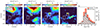 |
Fig. 6. Emission measure (EM) results applying the method by Plowman & Caspi (2020) on the original SDO/AIA data at 08:47:12 UT. Panels (a)–(d) show the EM maps integrated within the four distinct temperature bins specified in the respective labels. The white rectangle centered on (X, Y) = (41″, −94″) outlines the EUV counterpart of the UV burst, while the gray rectangle delimits a quiet region for comparison. Panel (e) contains the total EM within these two rectangles against temperature, where the associated errors are indicated as vertical lines. An animation of this figure is available online showing the time evolution from 08:35 to 09:00 UT. |
It is also interesting to note that the EM distributions of the UV burst and the quiet area are similar in terms of the shape and the temperature bin in which they reach their maximum. The relative EM enhancement at the burst location between log10(T[K]) = [6.0, 6.6] can be an indication that the temperature increase occurs in a higher-density plasma. We can estimate the density necessary to explain the enhanced EM at a given temperature bin. To that end, we suppose that the EM from the burst is a combination of the EM from the quiet region plus an extra optically thin layer, so
 (1)
(1)
where ne and nH are the electron and hydrogen number density, respectively. The plasma is totally ionized, so ne ≈ nH. If the plasma is uniform in this extra layer, we have
 (2)
(2)
where L is the length along the line-of-sight of the extra layer. Consequently,
 (3)
(3)
For instance, EMextra = 5 × 1027 cm−3 for the bin log10(T[K]) = [6.2, 6.3]. Assuming a length L ∈ [0.1, 1.0] Mm, this would imply ne ∈ [0.71, 2.24]×1010 cm−3, which corresponds to typical densities from the upper chromosphere and transition region. This is consistent with the UV burst happening below standard coronal heights. A detailed discussion regarding the EUV counterpart and the MK response is provided in Sect. 4.
3.5. The surge
Simultaneously with the UV burst, a chromospheric surge is ejected, which is an additional indication of magnetic reconnection. The surge is visible in the wings of Hα and Ca II K (see Fig. 1 and the associated animation) and reaches a maximum length and width of 8″ and 3″, respectively. The velocity inferred is around a few tens of km s−1 and its lifetime is approximately 19 min. The surge also shows a dark counterpart in all the SDO/AIA EUV channels, indicating that the surge thickness along the LOS has to be at least a few megameters to attenuate the AIA emission, as stated by Ortiz et al. (2016).
We inspected representative spectral profiles within the surge in Ca II K and relate them with the profiles obtained in Hα. The chosen locations to study the surge spectra are indicated in Fig. 1 by colored symbols: a blue diamond for surge plasma ascending and a red diamond for surge plasma descending. The results are shown in Fig. 7 following the same color-coding, including, as a black line, the average profile over the whole FOV for comparison purposes. Panel (a) shows that the Hα profiles are standard for a surge; in other words, they show blue- and redshift of the overall line profile, as well as asymmetry with enhanced absorption in one of the wings, in accordance to the motion of the plasma along the LOS. At the same location in Ca II K, panel (b), the ascending surge plasma shows an absent K2V peak, while the descending one has an absent K2R peak. We attribute this absence to the shift of the high-opacity Ca II K core (K3), which nearly completely blocks the photons coming from lower regions in the atmosphere that form the K2 features. This matches with the opacity window effect described for other chromospheric ejections such as spicules (Bose et al. 2019). The inferred K3 shifts, as well as the lower intensity K3 line minimum for the red profile, are in accordance with the corresponding Hα core Doppler shifts and relative intensities. This serves as a direct confirmation that the Ca II K3 feature is a good tracer of the LOS velocities in the chromosphere (see Bjørgen et al. 2018).
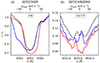 |
Fig. 7. Surge representative spectra for Hα (panel a) and Ca II K (panel b) at ∼08:48 UT. The blue and red curves are the profiles corresponding to the locations, respectively, indicated by the blue and red diamonds in Fig. 1. The black dashed line is a reference profile that is the average over the whole FOV of the observation. |
4. Discussion and conclusions
In this paper we used coordinated observations from SST, IRIS, and SDO obtained on 2017 May 25 to study the whole evolution of an ephemeral magnetic flux emergence episode and subsequent related energetic phenomena at the different solar atmospheric layers. In the following, we present the discussion and main conclusions for each of these phenomena from Sect. 3: the emerging bipole, the dark bubble, the EB, the UV burst, and the surge.
4.1. Magnetic flux emergence
The SST/CRISP magnetograms clearly reveal the appearance of a main bipole at the solar surface of a few arcseconds in size as well as other smaller bipoles emerging in the neighborhood. In contrast, the SDO/HMI magnetograms barely allow us to distinguish the positive part of the main bipole, substantially underestimating the amount of magnetic flux, even when incorporating the error deviation in the measurements. Deconvolving the SDO/HMI data (Norton et al. 2018) helps to obtain a slightly better agreement in the flux values and higher contrast in the magnetograms, but it is still not enough to clearly discern the main emerging bipole nor the smaller secondary magnetic flux emergence episodes that occur in the surroundings.
As a conclusion, our results show the importance of employing high-resolution magnetograms to detect small-scale magnetic flux emergence episodes and relate them to subsequent eruptive/ejective phenomena. Thus, we advise caution when using HMI magnetograms to draw conclusions about the origin of small-scale phenomena in the solar atmosphere. For instance, the claims about the lack of evidence of flux emergence leading to some surges (Nelson & Doyle 2013) or related to the campfires (Panesar et al. 2021, 2023) could be biased because of insufficient resolution. We estimate therefore that to properly resolve a bipole like the main one studied in this paper, it is necessary to have a resolution at least four to five times higher than that of HMI. This could be achievable, for example, using the Polarimetric and Helioseismic Imager (PHI; Solanki et al. 2020) on board SolO, which can reach 200 km resolution at a distance of 0.28 AU, or through ground-based telescopes with an aperture of at least 1 m.
4.2. The dark bubble
To the best of our knowledge, this is the first report in the Ca II K line of the existence of cold domes related to flux emergence through the appearance of a dark bubble located within the emerging bipole, and it adds to the already existing reports in Ca II H (Vargas Domínguez et al. 2012; Centeno et al. 2017; Kontogiannis et al. 2020), also referred to as dark lanes (Otsuji et al. 2007; Cheung et al. 2008; Guglielmino et al. 2010), and in the infrared Ca II 8542 Å line (Ortiz et al. 2014, 2016; de la Cruz Rodríguez et al. 2015b).
The reason for such intensity dimming in Ca II can be explained by adiabatic cooling that takes place when the emerging magnetized plasma rapidly expands as it rises through the solar atmosphere, as shown by de la Cruz Rodríguez et al. (2015b). Even though our results are not conclusive for Mg II h&k due to the location of the IRIS slit with respect to the bubble, it is encouraging to keep looking for evidence since these lines are formed higher in the solar atmosphere compared to the homologous Ca II H&K lines as well as the Ca II 8542 Å line (Leenaarts et al. 2013a,b; Bjørgen et al. 2018), and they could potentially track later stages of the expansion. Additionally, it would be of interest to explore other diagnostic methods that can provide information about cool temperatures, in a similar fashion to that used by Mulay & Fletcher (2021), through IRIS observations to find regions with H2 molecules next to flares, or as by Stauffer et al. (2022), employing observations in the 4.7 μm molecular band of CO with the NSO Array Camera (NAC; Ayres et al. 2008) to report cool features around a pore.
4.3. The Ellerman bomb
The reported EB following flux emergence appears to exhibit a very canonical pattern, with enhanced wings in both Hα and Ca II K, while the core of these lines remains relatively unperturbed. There is a 7-min delay between the EB and the appearance of the dark bubble, and an 11-min delay with respect to the first detection of the bipole. These timescales align with findings from 3D magneto-hydrodynamics (MHD) numerical simulations, which range from a few minutes (Danilovic 2017; Hansteen et al. 2017) to several tens of minutes (Danilovic et al. 2017; Hansteen et al. 2019). The delay is attributed to the time the emerged loops need to reach a few hundred kilometers above the surface and create a significant conflict with the pre-existing magnetic field in order to lead magnetic reconnection and plasma heating.
Recent observations using the Hβ line suggest that EBs are more common than previously believed, opening up new possibilities for the study of these small-scale reconnection events (Joshi & Rouppe van der Voort 2020b, 2022). The exact scenario to explain the high occurrence of EBs found in quiet sun (QS) regions remains unclear. Therefore, investigating the relationship between these quiet sun Ellerman bombs (QSEBs) and, for instance, flux emergence episodes as small as the secondary episodes reported here is a task that must be addressed in the near future: a challenge that can only be tackled with the availability of high-resolution magnetograms.
4.4. The UV burst
The UV burst following the EB displays canonical features, such as its size, its roundish shape, and an enhanced intensity with rapid temporal variation. Given the debate about the temperature and height formation of UV bursts (e.g., Judge 2015; Grubecka et al. 2016; Peter et al. 2019; Ni et al. 2022, and references therein), the finding of associated weak EUV signatures in the SDO/AIA coronal channels is particularly intriguing. Through DEM analysis, we show that the EUV response indicates heating above 1 MK temperatures. Additionally, the density estimated to explain the enhanced EUV related to the UV burst corresponds to densities between the upper chromosphere and transition region. These results are consistent with recent radiative MHD numerical models of magnetic flux emergence. There, UV bursts are formed in elongated current sheets spanning several scale heights through the chromosphere, and the plasma is at times heated to above 1 MK (see, e.g., Nóbrega-Siverio et al. 2017; Rouppe van der Voort et al. 2017; Hansteen et al. 2019). From observations it seems that there is a continuum of EUV counterparts concerning UV bursts, starting with Peter et al. (2014) and Kleint & Panos (2022), who did not find any counterparts in AIA images; then moving on to, for instance, Vissers et al. (2015) and Gupta & Tripathi (2015), who only detected brief signatures in the 171 and 193 Å filters; and finally to Guglielmino et al. (2018), who observed a very strong counterpart in the SDO/AIA coronal channels related to the UV burst, even reporting emission in the weak coronal Fe XII 1349.4 Å line using IRIS (Guglielmino et al. 2019). The diversity of EUV responses may stem from differences in the amount of magnetic energy involved during the flux emergence process and subsequent reconnection, as well as differences in the density of the inflow plasma at the reconnection site, which determines how efficient the Joule heating per particle is. Additionally, overlying cool and dense plasma to the reconnection site can also significantly absorb the EUV emission source, even blocking it completely (see Hansteen et al. 2019, and their Fig. 7).
Usually, in flux emergence experiments, there is a coronal inverted Y-shaped (or Eiffel-tower) jet with a narrow spine next to the surge once the plasma is heated to temperatures around MK (e.g., Yokoyama & Shibata 1995; Moreno-Insertis & Galsgaard 2013; Fang et al. 2014; Nóbrega-Siverio et al. 2016; Nóbrega-Siverio & Moreno-Insertis 2022). In our observations we did not detect such an elongated hot jet next to the surge. We cannot exclude that this is due to the resolution limitations of SDO/AIA and that we did not sufficiently spatially resolve the fine structure of this event. Nonetheless, we have seen that the bursty enhancements in the region of the UV burst detected in the SDO/AIA coronal channels occur on scales as small as 60 s. These timescales align with those recently reported by Chitta et al. (2023) concerning tiny inverted Y-shaped coronal jets with picoflare energy observed using SolO/EUI-HRI. It is likely that with higher resolution, some bursts could be associated with tiny EUV inverted Y-shaped jets.
4.5. The surge
The surge ejected as a result of magnetic flux emergence studied here shows typical values with respect to its properties. For instance, the surge has a lifetime of around 19 min, which fits with the values (between several minutes and tens of minutes) derived from observations (e.g., Wang et al. 2014; Ortiz et al. 2020; Guglielmino et al. 2018) and from simulations (e.g., Nóbrega-Siverio et al. 2016; Li et al. 2023). The velocities (around a few tens of km s−1) inferred from the shifts in the Hα and Ca II K lines are also in agreement with the moderate velocities that have been carefully analyzed in numerical experiments (see MacTaggart et al. 2015).
The fact that this surge is very canonical makes it a case study to start exploring their Ca II K properties. The motivation is that most of the observational surge studies have focused on Hα, and the ones studying the violet Ca II lines have been traditionally performed with broadband filters centered in Ca II H, for instance, using Hinode (Nishizuka et al. 2008; Liu et al. 2009, 2011). Consequently, the details about the Ca II K spectra have not been explored. In this paper we have made a first step to alleviate this, showing the Ca II K spectra in two representative locations of the surge. We find that the blue and red shifts seen in Hα in the surge have a corresponding counterpart as shifts of the Ca II K core (K3) with same Doppler velocities. This can potentially facilitate the surge identification using machine learning techniques in the near future, following approaches such as k-means (see, e.g., Nóbrega-Siverio et al. 2021).
4.6. Concluding remarks
We studied a unique dataset of coordinated observations between ground-based and space-borne telescopes covering the full evolution of an ephemeral magnetic flux emergence episode that triggers a chain of subsequent energetic phenomena higher in the atmosphere and ends with an eruption of plasma in the form of a surge. The high-resolution SST observations show in detail the emergence of a bipole that is practically impossible to discern in the cotemporal HMI magnetograms, emphasizing the need for high-resolution magnetograms to reveal the magnetic origin of small-scale atmospheric events. The emerging magnetic flux leads to the formation of a dark bubble, which is an imprint of the passage of the magnetized plasma traversing the low solar atmosphere and that is reported here in the Ca II K line for the first time. The observations also show the occurrence of magnetic reconnection once the emerging magnetized plasma interacts with the pre-existing magnetic field, as evidenced first by the appearance of an EB and then by a UV burst and surge, both with EUV counterparts. This provides an excellent scenario to compare with recent numerical MHD simulations. The EUV emission in the UV burst indicates heating to temperatures above 1 MK in the region of the upper chromosphere and transition region. We expect that forthcoming observations from SolO/EUI-HRI will provide valuable insights in this regard.
Movies
Movie 1 associated with Fig. 1 (figure_01) Access Supplementary Material
Movie 2 associated with Fig. 2 (figure_02) Access Supplementary Material
Movie 3 associated with Fig. 3 (figure_03) Access Supplementary Material
Movie 4 associated with Fig. 4 (figure_04) Access Supplementary Material
Movie 5 associated with Fig. 6 (figure_06) Access Supplementary Material
https://github.com/jaimedelacruz/pyMilne
http://hmi.stanford.edu/Description/hmi-overview/hmi-overview.html
https://robrutten.nl/rridl/00-README/sdo-manual.html
Acknowledgments
This research has been supported by the Spanish Ministry of Science, Innovation, and Universities through projects AYA2014-55078-P and PGC2018-095832-B-I00; by the European Research Council through the Synergy Grant number 810218 (ERC-2018-SyG); by the International Space Science Institute (ISSI) in Bern, through ISSI International Team project #535 Unraveling surges: a joint perspective from numerical models, observations, and machine learning; and by the Research Council of Norway through its Centres of Excellence scheme, project number 262622, and through project number 325491. S.B. gratefully acknowledges support from NASA grant 80NSSC20K1272 “Flux emergence and the structure, dynamics, and energetics of the solar atmosphere” and from NASA contract NNG09FA40C (IRIS). C.F. acknowledges funding from the CNES. The Swedish 1-m Solar Telescope is operated on the island of La Palma by the Institute for Solar Physics of Stockholm University in the Spanish Observatorio del Roque de Los Muchachos of the Instituto de Astrofísica de Canarias. The Institute for Solar Physics is supported by a grant for research infrastructures of national importance from the Swedish Research Council (registration number 2017-00625). IRIS is a NASA small explorer mission developed and operated by LMSAL with mission operations executed at NASA Ames Research center and major contributions to downlink communications funded by ESA and the Norwegian Space Centre. SDO observations are courtesy of NASA/SDO and the AIA, EVE, and HMI science teams. We acknowledge the HMI team for providing the data corrected for scattered light, with special thanks to Dr. Aimee Norton and Dr. Jeneen Sommers for their assistance.
References
- Athiray, P. S., & Winebarger, A. R. 2024, ApJ, 961, 181 [NASA ADS] [CrossRef] [Google Scholar]
- Ayres, T., Penn, M., Plymate, C., & Keller, C. 2008, Eur. Sol. Phys. Meeting, 12, 2.74 [NASA ADS] [Google Scholar]
- Berghmans, D., Auchère, F., Long, D. M., et al. 2021, A&A, 656, L4 [NASA ADS] [CrossRef] [EDP Sciences] [Google Scholar]
- Bjørgen, J. P., Sukhorukov, A. V., Leenaarts, J., et al. 2018, A&A, 611, A62 [Google Scholar]
- Bose, S., Henriques, V. M. J., Joshi, J., & Rouppe van der Voort, L. 2019, A&A, 631, L5 [NASA ADS] [CrossRef] [EDP Sciences] [Google Scholar]
- Bose, S., Joshi, J., Henriques, V. M. J., & Rouppe van der Voort, L. 2021, A&A, 647, A147 [EDP Sciences] [Google Scholar]
- Canfield, R. C., Reardon, K. P., Leka, K. D., et al. 1996, ApJ, 464, 1016 [NASA ADS] [CrossRef] [Google Scholar]
- Centeno, R., Blanco Rodríguez, J., Del Toro Iniesta, J. C., et al. 2017, ApJS, 229, 3 [NASA ADS] [CrossRef] [Google Scholar]
- Chen, Y., Tian, H., Peter, H., et al. 2019, ApJ, 875, L30 [NASA ADS] [CrossRef] [Google Scholar]
- Cheung, M. C. M., Schüssler, M., Tarbell, T. D., & Title, A. M. 2008, ApJ, 687, 1373 [Google Scholar]
- Chitta, L. P., Zhukov, A. N., Berghmans, D., et al. 2023, Science, 381, 867 [NASA ADS] [CrossRef] [Google Scholar]
- Danilovic, S. 2017, A&A, 601, A122 [NASA ADS] [CrossRef] [EDP Sciences] [Google Scholar]
- Danilovic, S., Solanki, S. K., Barthol, P., et al. 2017, ApJS, 229, 5 [NASA ADS] [CrossRef] [Google Scholar]
- de la Cruz Rodríguez, J. 2019, A&A, 631, A153 [NASA ADS] [CrossRef] [EDP Sciences] [Google Scholar]
- de la Cruz Rodríguez, J., Löfdahl, M. G., Sütterlin, P., Hillberg, T., & Rouppe van der Voort, L. 2015a, A&A, 573, A40 [NASA ADS] [CrossRef] [EDP Sciences] [Google Scholar]
- de la Cruz Rodríguez, J., Hansteen, V., Bellot-Rubio, L., & Ortiz, A. 2015b, ApJ, 810, 145 [Google Scholar]
- De Pontieu, B., Title, A. M., Lemen, J. R., et al. 2014, Sol. Phys., 289, 2733 [Google Scholar]
- Devi, P., Chandra, R., Awasthi, A. K., Schmieder, B., & Joshi, R. 2022, Sol. Phys., 297, 153 [NASA ADS] [CrossRef] [Google Scholar]
- Díaz Baso, C. J., de la Cruz Rodríguez, J., & Leenaarts, J. 2021, A&A, 647, A188 [NASA ADS] [CrossRef] [EDP Sciences] [Google Scholar]
- Dolliou, A., Parenti, S., Auchère, F., et al. 2023, A&A, 671, A64 [NASA ADS] [CrossRef] [EDP Sciences] [Google Scholar]
- Fang, F., Fan, Y., & McIntosh, S. W. 2014, ApJ, 789, L19 [NASA ADS] [CrossRef] [Google Scholar]
- Grubecka, M., Schmieder, B., Berlicki, A., et al. 2016, A&A, 593, A32 [NASA ADS] [CrossRef] [EDP Sciences] [Google Scholar]
- Guennou, C., Auchère, F., Soubrié, E., et al. 2012a, ApJS, 203, 25 [NASA ADS] [CrossRef] [Google Scholar]
- Guennou, C., Auchère, F., Soubrié, E., et al. 2012b, ApJS, 203, 26 [Google Scholar]
- Guglielmino, S. L., Bellot Rubio, L. R., Zuccarello, F., et al. 2010, ApJ, 724, 1083 [Google Scholar]
- Guglielmino, S. L., Zuccarello, F., Young, P. R., Murabito, M., & Romano, P. 2018, ApJ, 856, 127 [Google Scholar]
- Guglielmino, S. L., Young, P. R., & Zuccarello, F. 2019, ApJ, 871, 82 [Google Scholar]
- Gupta, G. R., & Tripathi, D. 2015, ApJ, 809, 82 [Google Scholar]
- Hannah, I. G., & Kontar, E. P. 2012, A&A, 539, A146 [NASA ADS] [CrossRef] [EDP Sciences] [Google Scholar]
- Hansteen, V. H., Archontis, V., Pereira, T. M. D., et al. 2017, ApJ, 839, 22 [NASA ADS] [CrossRef] [Google Scholar]
- Hansteen, V., Ortiz, A., Archontis, V., et al. 2019, A&A, 626, A33 [NASA ADS] [CrossRef] [EDP Sciences] [Google Scholar]
- Hashimoto, Y., Kitai, R., Ichimoto, K., et al. 2010, PASJ, 62, 879 [NASA ADS] [Google Scholar]
- Henriques, V. M. J. 2012, A&A, 548, A114 [NASA ADS] [CrossRef] [EDP Sciences] [Google Scholar]
- Huang, Z., Madjarska, M. S., Doyle, J. G., & Lamb, D. A. 2012, A&A, 548, A62 [NASA ADS] [CrossRef] [EDP Sciences] [Google Scholar]
- Huang, Z., Teriaca, L., Aznar Cuadrado, R., et al. 2023, A&A, 673, A82 [NASA ADS] [CrossRef] [EDP Sciences] [Google Scholar]
- Joshi, J., & Rouppe van der Voort, L. H. M. 2022, A&A, 664, A72 [NASA ADS] [CrossRef] [EDP Sciences] [Google Scholar]
- Joshi, R., Schmieder, B., Chandra, R., et al. 2017, Sol. Phys., 292, 152 [NASA ADS] [CrossRef] [Google Scholar]
- Joshi, R., Chandra, R., Schmieder, B., et al. 2020a, A&A, 639, A22 [NASA ADS] [CrossRef] [EDP Sciences] [Google Scholar]
- Joshi, J., Rouppe van der Voort, L. H. M., & de la Cruz Rodríguez, J. 2020b, A&A, 641, L5 [EDP Sciences] [Google Scholar]
- Judge, P. G. 2015, ApJ, 808, 116 [NASA ADS] [CrossRef] [Google Scholar]
- Kahil, F., Hirzberger, J., Solanki, S. K., et al. 2022, A&A, 660, A143 [NASA ADS] [CrossRef] [EDP Sciences] [Google Scholar]
- Kim, Y.-H., Yurchyshyn, V., Bong, S.-C., et al. 2015, ApJ, 810, 38 [NASA ADS] [CrossRef] [Google Scholar]
- Kleint, L., & Panos, B. 2022, A&A, 657, A132 [NASA ADS] [CrossRef] [EDP Sciences] [Google Scholar]
- Kontogiannis, I., Tsiropoula, G., Tziotziou, K., et al. 2020, A&A, 633, A67 [NASA ADS] [CrossRef] [EDP Sciences] [Google Scholar]
- Kosugi, T., Matsuzaki, K., Sakao, T., et al. 2007, Sol. Phys., 243, 3 [Google Scholar]
- Leenaarts, J., Pereira, T. M. D., Carlsson, M., Uitenbroek, H., & De Pontieu, B. 2013a, ApJ, 772, 89 [NASA ADS] [CrossRef] [Google Scholar]
- Leenaarts, J., Pereira, T. M. D., Carlsson, M., Uitenbroek, H., & De Pontieu, B. 2013b, ApJ, 772, 90 [NASA ADS] [CrossRef] [Google Scholar]
- Leenaarts, J., de la Cruz Rodríguez, J., Danilovic, S., Scharmer, G., & Carlsson, M. 2018, A&A, 612, A28 [NASA ADS] [CrossRef] [EDP Sciences] [Google Scholar]
- Lemen, J. R., Title, A. M., Akin, D. J., et al. 2012, Sol. Phys., 275, 17 [Google Scholar]
- Li, X., Keppens, R., & Zhou, Y. 2023, ApJ, 947, L17 [NASA ADS] [CrossRef] [Google Scholar]
- Liu, Y., & Kurokawa, H. 2004, ApJ, 610, 1136 [Google Scholar]
- Liu, W., Berger, T. E., Title, A. M., & Tarbell, T. D. 2009, ApJ, 707, L37 [NASA ADS] [CrossRef] [Google Scholar]
- Liu, W., Berger, T. E., Title, A. M., Tarbell, T. D., & Low, B. C. 2011, ApJ, 728, 103 [NASA ADS] [CrossRef] [Google Scholar]
- Liu, Y., Hoeksema, J. T., Scherrer, P. H., et al. 2012, Sol. Phys., 279, 295 [Google Scholar]
- Löfdahl, M. G., Hillberg, T., de la Cruz Rodríguez, J., et al. 2021, A&A, 653, A68 [Google Scholar]
- MacTaggart, D., Guglielmino, S. L., Haynes, A. L., Simitev, R., & Zuccarello, F. 2015, A&A, 576, A4 [NASA ADS] [CrossRef] [EDP Sciences] [Google Scholar]
- Mandal, S., Chitta, L. P., Peter, H., et al. 2022, A&A, 664, A28 [NASA ADS] [CrossRef] [EDP Sciences] [Google Scholar]
- Moreno-Insertis, F., & Galsgaard, K. 2013, ApJ, 771, 20 [Google Scholar]
- Mulay, S. M., & Fletcher, L. 2021, MNRAS, 504, 2842 [NASA ADS] [CrossRef] [Google Scholar]
- Müller, D., St. Cyr, O. C., Zouganelis, I., et al. 2020, A&A, 642, A1 [Google Scholar]
- Nelson, C. J., & Doyle, J. G. 2013, A&A, 560, A31 [NASA ADS] [CrossRef] [EDP Sciences] [Google Scholar]
- Nelson, C. J., Doyle, J. G., Erdélyi, R., et al. 2013, Sol. Phys., 283, 307 [Google Scholar]
- Ni, L., Cheng, G., & Lin, J. 2022, A&A, 665, A116 [NASA ADS] [CrossRef] [EDP Sciences] [Google Scholar]
- Nishizuka, N., Shimizu, M., Nakamura, T., et al. 2008, ApJ, 683, L83 [NASA ADS] [CrossRef] [Google Scholar]
- Nóbrega-Siverio, D., & Moreno-Insertis, F. 2022, ApJ, 935, L21 [CrossRef] [Google Scholar]
- Nóbrega-Siverio, D., Moreno-Insertis, F., & Martínez-Sykora, J. 2016, ApJ, 822, 18 [Google Scholar]
- Nóbrega-Siverio, D., Martínez-Sykora, J., Moreno-Insertis, F., & Rouppe van der Voort, L. 2017, ApJ, 850, 153 [CrossRef] [Google Scholar]
- Nóbrega-Siverio, D., Guglielmino, S. L., & Sainz Dalda, A. 2021, A&A, 655, A28 [CrossRef] [EDP Sciences] [Google Scholar]
- Norton, A. A., Duvall, T. L., Jr., Schou, J., et al. 2018, Catalyzing Solar Connections, 101 [Google Scholar]
- Ortiz, A., Bellot Rubio, L. R., Hansteen, V. H., de la Cruz Rodríguez, J., & Rouppe van der Voort, L. 2014, ApJ, 781, 126 [NASA ADS] [CrossRef] [Google Scholar]
- Ortiz, A., Hansteen, V. H., Bellot Rubio, L. R., et al. 2016, ApJ, 825, 93 [NASA ADS] [CrossRef] [Google Scholar]
- Ortiz, A., Hansteen, V. H., Nóbrega-Siverio, D., & Rouppe van der Voort, L. 2020, A&A, 633, A58 [NASA ADS] [CrossRef] [EDP Sciences] [Google Scholar]
- Otsuji, K., Shibata, K., Kitai, R., et al. 2007, PASJ, 59, S649 [NASA ADS] [Google Scholar]
- Panesar, N. K., Tiwari, S. K., Berghmans, D., et al. 2021, ApJ, 921, L20 [CrossRef] [Google Scholar]
- Panesar, N. K., Hansteen, V. H., Tiwari, S. K., et al. 2023, ApJ, 943, 24 [NASA ADS] [CrossRef] [Google Scholar]
- Pariat, E., Aulanier, G., Schmieder, B., et al. 2004, ApJ, 614, 1099 [Google Scholar]
- Pesnell, W. D., Thompson, B. J., & Chamberlin, P. C. 2012, Sol. Phys., 275, 3 [Google Scholar]
- Peter, H., Tian, H., Curdt, W., et al. 2014, Science, 346, 1255726 [Google Scholar]
- Peter, H., Huang, Y. M., Chitta, L. P., & Young, P. R. 2019, A&A, 628, A8 [NASA ADS] [CrossRef] [EDP Sciences] [Google Scholar]
- Plowman, J., & Caspi, A. 2020, ApJ, 905, 17 [NASA ADS] [CrossRef] [Google Scholar]
- Press, W. H., Teukolsky, S. A., Vetterling, W. T., & Flannery, B. P. 1992, Numerical Recipes in FORTRAN. The Art of Scientific Computing, 2nd ed. (Cambridge: University Press) [Google Scholar]
- Reid, A., Mathioudakis, M., Doyle, J. G., et al. 2016, ApJ, 823, 110 [Google Scholar]
- Rochus, P., Auchère, F., Berghmans, D., et al. 2020, A&A, 642, A8 [NASA ADS] [CrossRef] [EDP Sciences] [Google Scholar]
- Rouppe van der Voort, L., De Pontieu, B., Scharmer, G. B., et al. 2017, ApJ, 851, L6 [Google Scholar]
- Rouppe van der Voort, L. H. M., De Pontieu, B., Carlsson, M., et al. 2020, A&A, 641, A146 [EDP Sciences] [Google Scholar]
- Rouppe van der Voort, L. H. M., Joshi, J., Henriques, V. M. J., & Bose, S. 2021, A&A, 648, A54 [NASA ADS] [CrossRef] [EDP Sciences] [Google Scholar]
- Rouppe van der Voort, L. H. M., van Noort, M., & de la Cruz Rodríguez, J. 2023, A&A, 673, A11 [NASA ADS] [CrossRef] [EDP Sciences] [Google Scholar]
- Ruan, G., Schmieder, B., Masson, S., et al. 2019, ApJ, 883, 52 [NASA ADS] [CrossRef] [Google Scholar]
- Rutten, R. J., Vissers, G. J. M., Rouppe van der Voort, L. H. M., Sütterlin, P., & Vitas, N. 2013, J. Phys. Conf. Ser., 440, 012007 [Google Scholar]
- Scharmer, G. B., Bjelksjo, K., Korhonen, T. K., Lindberg, B., & Petterson, B. 2003, in Innovative Telescopes and Instrumentation for Solar Astrophysics, eds. S. L. Keil, & S. V. Avakyan, SPIE Conf. Ser., 4853, 341 [NASA ADS] [CrossRef] [Google Scholar]
- Scharmer, G. B., Narayan, G., Hillberg, T., et al. 2008, ApJ, 689, L69 [Google Scholar]
- Scharmer, G. B., Sliepen, G., Sinquin, J.-C., et al. 2024, A&A, 685, A32 [NASA ADS] [CrossRef] [EDP Sciences] [Google Scholar]
- Scherrer, P. H., Schou, J., Bush, R. I., et al. 2012, Sol. Phys., 275, 207 [Google Scholar]
- Schmieder, B., Guo, Y., Moreno-Insertis, F., et al. 2013, A&A, 559, A1 [NASA ADS] [CrossRef] [EDP Sciences] [Google Scholar]
- Shen, J., Xu, Z., Li, J., & Ji, H. 2022, ApJ, 925, 46 [NASA ADS] [CrossRef] [Google Scholar]
- Shibata, K., Ishido, Y., Acton, L. W., et al. 1992, PASJ, 44, L173 [Google Scholar]
- Solanki, S. K., Riethmüller, T. L., Barthol, P., et al. 2017, ApJS, 229, 2 [NASA ADS] [CrossRef] [Google Scholar]
- Solanki, S. K., del Toro Iniesta, J. C., Woch, J., et al. 2020, A&A, 642, A11 [NASA ADS] [CrossRef] [EDP Sciences] [Google Scholar]
- Stauffer, J. R., Reardon, K. P., & Penn, M. 2022, ApJ, 930, 87 [NASA ADS] [CrossRef] [Google Scholar]
- Su, Y., Veronig, A. M., Hannah, I. G., et al. 2018, ApJ, 856, L17 [NASA ADS] [CrossRef] [Google Scholar]
- Tian, H., Yurchyshyn, V., Peter, H., et al. 2018, ApJ, 854, 92 [Google Scholar]
- Tsuneta, S., Ichimoto, K., Katsukawa, Y., et al. 2008, Sol. Phys., 249, 167 [Google Scholar]
- Van Noort, M., Der Voort, L. R. V., & Löfdahl, M. G. 2005, Sol. Phys., 228, 191 [NASA ADS] [CrossRef] [Google Scholar]
- Vargas Domínguez, S., van Driel-Gesztelyi, L., & Bellot Rubio, L. R. 2012, Sol. Phys., 278, 99 [CrossRef] [Google Scholar]
- Vargas Domínguez, S., Kosovichev, A., & Yurchyshyn, V. 2014, ApJ, 794, 140 [CrossRef] [Google Scholar]
- Verma, M., Denker, C., Diercke, A., et al. 2020, A&A, 639, A19 [NASA ADS] [CrossRef] [EDP Sciences] [Google Scholar]
- Viall, N. M., & Klimchuk, J. A. 2015, ApJ, 799, 58 [NASA ADS] [CrossRef] [Google Scholar]
- Vissers, G. J. M., Rouppe van der Voort, L. H. M., & Rutten, R. J. 2013, ApJ, 774, 32 [NASA ADS] [CrossRef] [Google Scholar]
- Vissers, G. J. M., Rouppe van der Voort, L. H. M., Rutten, R. J., Carlsson, M., & De Pontieu, B. 2015, ApJ, 812, 11 [NASA ADS] [CrossRef] [Google Scholar]
- Vissers, G. J. M., Rouppe van der Voort, L. H. M., & Rutten, R. J. 2019a, A&A, 626, A4 [NASA ADS] [CrossRef] [EDP Sciences] [Google Scholar]
- Vissers, G. J. M., de la Cruz Rodríguez, J., Libbrecht, T., et al. 2019b, A&A, 627, A101 [NASA ADS] [CrossRef] [EDP Sciences] [Google Scholar]
- Wang, J.-f., Zhou, T.-h., & Ji, H.-s. 2014, Chin. Astron. Astrophys., 38, 65 [CrossRef] [Google Scholar]
- Watanabe, H., Vissers, G., Kitai, R., Rouppe van der Voort, L., & Rutten, R. J. 2011, ApJ, 736, 71 [NASA ADS] [CrossRef] [Google Scholar]
- Yang, H., Chae, J., Lim, E.-K., et al. 2016, ApJ, 829, 100 [NASA ADS] [CrossRef] [Google Scholar]
- Yokoyama, T., & Shibata, K. 1995, Nature, 375, 42 [Google Scholar]
- Young, P. R., Tian, H., Peter, H., et al. 2018, Space Sci. Rev., 214, 120 [Google Scholar]
- Zhukov, A. N., Mierla, M., Auchère, F., et al. 2021, A&A, 656, A35 [NASA ADS] [CrossRef] [EDP Sciences] [Google Scholar]
- Zwaan, C. 1987, ARA&A, 25, 83 [NASA ADS] [CrossRef] [Google Scholar]
All Figures
|
Fig. 1. Coordinated observations on 2017 May 25 at ∼08:48 UT. Panel (a): LOS magnetogram for SST/CRISP. Panel (b): Hα at −32 km s−1 from SST/CRISP. Panel (c): IRIS/SJI 1400 Å aligned to SST. Panel (d): SDO/AIA 193 Å aligned to SST. The 19″ × 19″ field of view highlighted in green encompasses the region of interest shown in the rest of the panels. Panels (e) and (f): LOS magnetograms for SST/CRISP and SDO/HMI aligned to SST, respectively. The red rectangle delimits the area where magnetic flux is analyzed in Sect. 3.1. Panel (g): Hα at −32 km s−1 from SST/CRISP. The colored diamonds indicate the location of the spectral profiles shown in Sect. 3.5. Panel (h): Ca II K at 10 km s−1 taken with SST/CHROMIS. Panel (i): IRIS/SJI 1400 Å with eight lines indicating the approximate locations of the spectrograph slit and the area covered by the raster scan. The light curves within the light gray rectangle are studied in Sect. 3.4. Panels (j), (k), and (l): SDO/AIA 171 Å, 193 Å, and 211 Å, respectively. In all the zoomed-in panels, the colored contours delimit the surge in the Hα blue wing (blue) and the UV burst on the IRIS/SJI 1400 (green). An animation of this figure is available online with the evolution of the system from 08:15 to 09:02 UT. |
| In the text | |
|
Fig. 2. Magnetic flux emergence episode. Panels (a) and (b): LOS magnetograms, respectively, from SST/CRISP and SDO/HMI aligned to SST. Panels (c) and (d): LOS magnetograms from the original SDO/HMI data without and with deconvolution, respectively. Panels (e), (f), (g), and (h): Magnetic flux evolution within the red rectangle for the corresponding magnetograms, showing the unsigned flux (black), the positive flux (blue), and the absolute value of the negative flux (red). In panels (e) and (g), the gray band represents the standard deviation of the unsigned flux measured in the original SST/CRISP and SDO/HMI data, respectively. An animation of this figure is available online showing the time evolution from 08:07 to 08:59 UT. |
| In the text | |
|
Fig. 3. Dark bubble. Panel (a): LOS magnetogram from SST/CRISP. Panel (b): Ca II K map at −49 km s−1 from SST/CHROMIS. Panel (c): Ca II K profiles normalized to the continuum for the location marked in panel (b) (solid line), and the average over the whole FOV of the observation (dashed line). Panel (d): Time evolution of the normalized Ca II K intensity at −49 km s−1 for the position indicated in panel (b) (orange), and the unsigned magnetic flux from SST/CRISP within the red rectangle (black). An animation of this figure is available online showing the time evolution from 08:07 to 08:59 UT. |
| In the text | |
|
Fig. 4. Ellerman Bomb. Panels (a) and (e): Maps of the Hα and Ca II K lines, respectively, in the far-blue wing. The location of the EB centered at (9.″8, 11.″8) is indicated with a circle. Panels (b) and (f): λ − t plot at the center of the EB for Hα and Ca II K, respectively. The vertical red line indicates the spectral position shown in panels (a) and (e), while the horizontal green line indicates the time. Panels (c) and (g): Comparison between the spectral profile of the EB (solid) and the average profile over the whole FOV of the observation (dashed) for Hα and Ca II K, respectively. Panels (d) and (h): SDO/AIA 1600 and 1700 Å channels aligned to SST. An animation of this figure is available online showing the time evolution from 08:25 to 08:35 UT. |
| In the text | |
|
Fig. 5. Standardized intensity calculated within the light gray rectangle shown in Fig. 1. The curve from IRIS (left axis) shows the UV burst in SJI 1400 Å (black), whereas the curves from SDO (right axis) depict its EUV counterpart in the AIA filters 94 Å (green), 193 Å (red), 171 Å (yellow), and 211 Å (blue). |
| In the text | |
|
Fig. 6. Emission measure (EM) results applying the method by Plowman & Caspi (2020) on the original SDO/AIA data at 08:47:12 UT. Panels (a)–(d) show the EM maps integrated within the four distinct temperature bins specified in the respective labels. The white rectangle centered on (X, Y) = (41″, −94″) outlines the EUV counterpart of the UV burst, while the gray rectangle delimits a quiet region for comparison. Panel (e) contains the total EM within these two rectangles against temperature, where the associated errors are indicated as vertical lines. An animation of this figure is available online showing the time evolution from 08:35 to 09:00 UT. |
| In the text | |
|
Fig. 7. Surge representative spectra for Hα (panel a) and Ca II K (panel b) at ∼08:48 UT. The blue and red curves are the profiles corresponding to the locations, respectively, indicated by the blue and red diamonds in Fig. 1. The black dashed line is a reference profile that is the average over the whole FOV of the observation. |
| In the text | |
Current usage metrics show cumulative count of Article Views (full-text article views including HTML views, PDF and ePub downloads, according to the available data) and Abstracts Views on Vision4Press platform.
Data correspond to usage on the plateform after 2015. The current usage metrics is available 48-96 hours after online publication and is updated daily on week days.
Initial download of the metrics may take a while.