| Issue |
A&A
Volume 677, September 2023
|
|
|---|---|---|
| Article Number | A182 | |
| Number of page(s) | 28 | |
| Section | Planets and planetary systems | |
| DOI | https://doi.org/10.1051/0004-6361/202346692 | |
| Published online | 27 September 2023 | |
Two super-Earths at the edge of the habitable zone of the nearby M dwarf TOI-2095★
1
Instituto de Astrofisica de Canarias (IAC),
38205
La Laguna, Tenerife, Spain
e-mail: This email address is being protected from spambots. You need JavaScript enabled to view it.
2
Departamento de Astrofisica, Universidad de La Laguna (ULL),
38206
La Laguna, Tenerife, Spain
3
Centro de Astrobiologia (CSIC-INTA),
ESAC campus,
28692
Villanueva de la Canada (Madrid), Spain
4
NASA Exoplanet Science Institute-Caltech/IPAC,
Pasadena, CA
91125, USA
5
University of California Santa Cruz,
Santa Cruz, CA
95065, USA
6
Sternberg Astronomical Institute, M.V. Lomonosov Moscow State University,
13, Universitetskij pr.,
119234
Moscow, Russia
7
Center for Astrophysics | Harvard & Smithsonian,
60 Garden Street,
Cambridge, MA
02138, USA
8
Department of Astronomy and Tsinghua Centre for Astrophysics, Tsinghua University,
Beijing
100084, PR China
9
Campo Catino Astronomical Observatory,
Regione Lazio, Guarcino (FR)
03010, Italy
10
Lund Observatory, Division of Astrophysics, Department of Physics, Lund University,
PO Box 43,
22100
Lund, Sweden
11
Komaba Institute for Science, The University of Tokyo,
3-8-1 Komaba, Meguro,
Tokyo
153-8902, Japan
12
Astrobiology Center,
2-21-1 Osawa, Mitaka,
Tokyo
181-8588, Japan
13
Department of Multi-Disciplinary Sciences, Graduate School of Arts and Sciences, The University of Tokyo,
3-8-1 Komaba, Meguro,
Tokyo
153-8902, Japan
14
Instituto de Astrofisica de Andalucia (IAA-CSIC),
Glorieta de la Astronomia s/n,
18008
Granada, Spain
15
Max-Planck-Institut für Astronomie,
Königstuhl 17,
69117
Heidelberg, Germany
16
Department of Astronomy and Astrophysics, University of Chicago,
Chicago, IL
60637, USA
17
Landessternwarte, Zentrum für Astronomie der Universität Heidelberg,
Königstuhl 12,
69117
Heidelberg, Germany
18
Institut für Astrophysik und Geophysik, Georg-August-Universität,
Friedrich-Hund-Platz 1,
37077
Göttingen, Germany
19
Institut de Ciències de l’Espai (CSIC),
Campus UAB, c/ de Can Magrans s/n,
08193
Bellaterra, Barcelona, Spain
20
Institut d’Estudis Espacials de Catalunya,
08034
Barcelona, Spain
21
Hamburger Sternwarte, Universität Hamburg,
Gojenbergsweg 112,
21029
Hamburg, Germany
22
Department of Physics and Kavli Institute for Astrophysics and Space Research, Massachusetts Institute of Technology,
Cambridge, MA
02139, USA
23
Steward Observatory and Department of Astronomy, The University of Arizona,
Tucson, AZ
85721, USA
24
Vereniging Voor Sterrenkunde (VVS),
Oostmeers 122 C,
8000
Brugge, Belgium
25
Centre for Mathematical Plasma-Astrophysics, Department of Mathematics, KU Leuven,
Celestijnenlaan 200B,
3001
Heverlee, Belgium
26
Public Observatory ASTROLAB IRIS, Provinciaal Domein “De Palingbeek”,
Verbrandemolenstraat 5,
8902
Zillebeke, Ieper, Belgium
27
Department of Earth, Atmospheric, and Planetary Sciences, Massachusetts Institute of Technology,
Cambridge, MA
02139, USA
28
Department of Aeronautics and Astronautics, Massachusetts Institute of Technology,
Cambridge, MA
02139, USA
29
NASA Ames Research Center,
Moffett Field, CA
94035, USA
30
Department of Astrophysical Sciences, Princeton University,
Princeton, NJ
08544, USA
31
Department of Space, Earth and Environment, Chalmers University of Technology,
412 96
Gothenburg, Sweden
Received:
18
April
2023
Accepted:
26
July
2023
Abstract
The main scientific goal of TESS is to find planets smaller than Neptune around stars that are bright enough to allow for further characterization studies. Given our current instrumentation and detection biases, M dwarfs are prime targets in the search for small planets that are in (or near) the habitable zone of their host star. In this work, we use photometric observations and CARMENES radial velocity (RV) measurements to validate a pair of transiting planet candidates found by TESS. The data were fitted simultaneously, using a Bayesian Markov chain Monte Carlo (MCMC) procedure and taking into account the stellar variability present in the photometric and spectroscopic time series. We confirm the planetary origin of the two transiting candidates orbiting around TOI-2095 (LSPM J1902+7525). The star is a nearby M dwarf (d = 41.90 ± 0.03 pc, Teff = 3759 ± 87 K, V = 12.6 mag), with a stellar mass and radius of M* = 0.44 ± 0.02 M⊙ and R* = 0.44 ± 0.02 R⊙, respectively. The planetary system is composed of two transiting planets: TOI-2095b, with an orbital period of Pb = 17.66484 ± (7 × 10⁻⁵) days, and TOI-2095c, with Pc = 28.17232 ± (14 × 10−5) days. Both planets have similar sizes with Rb = 1.25 ± 0.07 R⊕ and Rc = 1.33 ± 0.08 R⊕ for planet b and planet c, respectively. Although we did not detect the induced RV variations of any planet with significance, our CARMENES data allow us to set stringent upper limits on the masses of these objects. We find Mb < 4.1 M⊕ for the inner and Mc < 7.4 M⊕ for the outer planet (95% confidence level). These two planets present equilibrium temperatures in the range of 300–350 K and are close to the inner edge of the habitable zone of their star.
Key words: planets and satellites: detection / techniques: photometric / techniques: radial velocities
Radial velocity measurement table is available at the CDS via anonymous ftp to cdsarc.cds.unistra.fr (130.79.128.5) or via https://cdsarc.cds.unistra.fr/viz-bin/cat/J/A+A/677/A182
© The Authors 2023
 Open Access article, published by EDP Sciences, under the terms of the Creative Commons Attribution License (https://creativecommons.org/licenses/by/4.0), which permits unrestricted use, distribution, and reproduction in any medium, provided the original work is properly cited.
This article is published in open access under the Subscribe to Open model. This email address is being protected from spambots. You need JavaScript enabled to view it. to support open access publication.
1 Introduction
Due to their relatively small masses and sizes, M dwarfs are prime targets in the search for small (Rp ~ 1–4 R⊕) planets using current detection techniques. Furthermore, it is likely that the only rocky worlds around main sequence stars whose atmospheres we will be able to study over the next decade are transiting planets detected around late-type stars (e.g., Batalha et al. 2018). Among the more than 5400 planets detected to date, fewer than 300 have been found to be transiting around M dwarfs1. With such a small sample size, it is not surprising to see that there are close to 30 known exoplanets around M dwarfs that are in the habitable zone (HZ) of their star (Martínez-Rodríguez et al. 2019) – and only about ten of those planets are transiting (e.g., Kepler-186f, Quintana et al. 2014; TRAPPIST-1e, -1f, -1g, Gillon et al. 2016, 2017; Kepler-1652b, Torres et al. 2017; LHS 1140b, Dittmann et al. 2017; Lillo-Box et al. 2020; K2-288B b, Feinstein et al. 2019; TOI-700d, Rodriguez et al. 2020; LP 890-9 c, Delrez et al. 2022). There is also the late-K-dwarf HZ desert pointed out by Lillo-Box et al. (2022) that is of interest. We note that although the true habitability of M dwarfs has been highly debated in great part due to their frequent and energetic flares (Shields et al. 2016), it has been shown that stellar activity and magnetic flaring is dramatically diminished for stars earlier than M3 V. We refer to Hilton et al. (2010), Jeffers et al. (2018), and Günther et al. (2020) for a more recent analysis using TESS data.
Due to the possibility of detecting biomarkers in their atmospheres using transmission spectroscopy, this select group of transiting planets will be the subject of intensive observing campaigns with facilities such as JWST (Gardner et al. 2006). Temperate planets located at the predicted edges of the HZ of their host stars are also excellent targets for detailed atmospheric studies to better understand processes such as the runaway greenhouse effect (Ingersoll 1969; Kasting 1988) as well as to test the predicted theoretical limits of the habitable zone (e.g., Kopparapu et al. 2013; Zsom et al. 2013; Turbet et al. 2019).
In addition to their prospects for atmospheric characterization, studying small planets can help improve the understanding of the global picture of planet populations found in our galaxy. Fulton et al. (2017) showed that the size distributions of small planets with orbital periods of less than 100 days present a bimodal distribution, presumably representing two general groups: rocky planets with none or small scale atmospheres (Rp ~ 1 – 2 R⊕) and planets with considerable gaseous envelopes and sizes in the range Rp - 2-4 Re. The origin of this separation of planet populations has been attributed to atmospheric mass loss processes (e.g., Owen & Wu 2013; Lopez & Rice 2018; Mordasini 2020). The position of the gap between both distributions (at around Rp ~ 1.7 R⊕) has been found to be dependent on planetary orbital period, the stellar flux received by the planet, and even the stellar type of the host star (e.g., Martinez et al. 2019; Wu 2019). Recently, Luque & Pallé (2022) suggested that for planets around M dwarfs, the bimodal distribution of planetary radii is better explained by density classes, with three populations comprised of rocky, water-rich (i.e., water worlds), and gaseous planets – rather than by a separation between rocky and gas-rich planets. To obtain a more comprehensive picture, it is necessary to increase the sample of small transiting planets with mass estimates.
In this work, we report the discovery and validation of two small (Rp ~ 1.2–1.3 R⊕) transiting planets around the M dwarf TOI-2095. The planets were found and announced to the community by the Transiting Exoplanet Survey Satellite (TESS). The host star is a nearby M dwarf (d = 41.90 ± 0.03 pc; Bailer-Jones et al. 2021) that is relatively bright in the near infrared (V = 12.7 mag, J = 9.8 mag). We use space- and ground-based observations to establish the radius and put upper limits on the masses of both transiting planets.
This paper is structured as follows. In Sect. 2, we describe TESS observations, in Sect. 3 we describe the ground-based imaging and spectroscopic observations of the star, and in Sect. 4 we present the stellar properties of the host star. In Sect. 5, we describe our data fitting procedure and the results of our analysis. In Sect. 6, we discuss the search for more transiting planets in TESS data, in Sect. 7, we discuss the dynamical stability of the system, and in Sect. 8, we present a discussion of the characteristics of the planets around TOI-2095. Finally, in Sect. 9 we present our conclusions.
2 TESS photometry
TESS (Ricker et al. 2014) is a NASA space-based observatory dedicated to search the entire sky for new transiting planets around bright stars. The satellite observes an area of the sky of 24° × 96° continuously for ~27 days sending data to Earth every ~13.7 days. The data analysis process of the TESS Science Processing Operations Center (SPOC; Jenkins et al. 2016) at the NASA Ames Research Center consists of generating light curves using simple aperture photometry (SAP; Morris et al. 2020) that are then removed of systematic effects using the Presearch Data Conditioning (PDC) pipeline module (Smith et al. 2012; Stumpe et al. 2012, 2014). The resulting photometric time series are then searched to identify transit events with a wavelet-based matched filter (Jenkins 2002; Li et al. 2019; Jenkins et al. 2020), and tests are applied to rule out some non-planetary scenarios (Twicken et al. 2018). After this process, TESS Science Office (TSO) at MIT reviews the vetting reports and which transit-like signatures should be promoted to planet candidate status. On 15 July 2020, the TSO alerted to the community the detection of two distinct transiting signal on TOI-2095. The detected signals have a period of P = 17.6649 days with a transit depth of 670 ppm (0.72 mmag) and P = 28.1723 days with a depth of 820 ppm (0.89 mmag). The candidates were assigned a TESS object of interest (TOI) number of TOI-2095.01 (TOI-2095b, hereafter) and TOI-2095.02 (TOI-2095c from now on) for the P ~ 17 day and P ~ 28 day signals, respectively.
In this work, we analyzed a total of 22 TESS sectors (PDC-SAP photometry) taken with a 2 min cadence for the star TOI-2095 (TIC 235678745). The data were taken from 18 July 2019 to 4 July 2020 (Sectors 14 to 26), from 28 June 2021 to 20 August 2021 (Sectors 40 and 41), and from 30 December 2021 to 1 September 2022 (Sectors 47 to 55). We excluded data from Sector 54 from the analysis, since the PDCSAP light curve presented a poor correction of the instrumental systematics when compared to the rest of available observations. The target pixel files showing the TESS apertures used to compute the photometric time series are shown in Fig. A.1.
3 Ground-based observations
3.1 Seeing-limited photometry
3.1.1 Long-term photometric monitoring
TOI-2095 was observed using the 0.8 m Joan Oró Telescope (TJO) at the Observatori Astronòmic del Montsec (OAdM), Sant Esteve de la Sarga, Catalonia, Spain as a part of a photometric monitoring campaign of TESS targets. The objective of the observations was to establish the rotational period of the star from photometric variations. To obtain the data, we used TJO LAIA 4k×4k CCD camera with a field of view of 30′ (pixel scale of 0.4″ pixel−1). The photometric observations were obtained using the Johnson R filter, with an exposure time of 120 s. A standard data reduction was performed with the icat pipeline (Colome & Ribas 2006) and differential aperture photometry was done with AstroImageJ (Collins et al. 2017). From TJO, we collected a total of 759 epochs with a time baseline of ~589 days.
We also searched for archival data on public photometric data bases. We obtained Zwicky Transient Facility (ZTF; Masci et al. 2019) observations of TOI-2095 taken with the 48-inch Samuel Oschin Telescope at the Palomar Observatory, USA. It uses an array of 16 6k×6k to cover a field of view of 47 square degrees (pixel scale of 1.0″ pixel−1) and the data are taken with the Sloan z filter. After removing some outliers using a sigma-clipping procedure (3σ threshold), we analyzed a total of 390 epochs spanning a time baseline of ~1333 days.
3.1.2 OACC transit photometry
An ingress of TOI-2095b was observed on 23 August 2020 with the 0.35 m Planewave telescope at the remotely controlled Campo Catino Rodeo Observatory (OACC-Rodeo) located in Rodeo, New Mexico, USA. The telescope is equipped with a FLI KAF50100 camera with 8176 x 6132 pixels and a field of view of 17′ (pixel scale of 0.48″ pixel−1). The observations were taken with a clear filter and with an exposure time of 180 s. The data reduction and aperture photometry was done using AstroImageJ (Collins et al. 2017). The data covered the ingress and almost the full predicted transit. The transit event was too shallow to be detected but the observations discarded eclipsing binaries (EBs) around the target star in a 3′ radius as possible sources of the transit signal detected by TESS.
3.1.3 LCOGT transit photometry
Two transit events were observed by Las Cumbres Observatory Global Telescope Network (LCOGT; Brown et al. 2013) using its 1 m telescopes. We used the TESS Transit Finder, which is a customized version of the Tapir software package (Jensen 2013), to schedule our transit observations. LCOGT 1 m telescopes are equipped with Sinistra cameras with a field of view of 26′ × 26′ and a pixel scale of 0.389″ pixel−1. A transit of TOI-2095c was observed at the LCOGT McDonald Observatory node in Jeff Davis County, Texas, USA, on the night of 6 September 2020. The observations were made using the Sloan i′ filter with an exposure time of 35 s (Fig. B.1). A transit of TOI-2095b was observed from Observatorio del Teide, Tenerife, Spain on 21 June 2022. The data were acquired using the Sloan i′ band and with an exposure time of 40 s (Fig. B.2). The raw images were processed with LCOGT’s pipeline BANZAI (McCully et al. 2018), which performs standard dark and flat-field corrections. The aperture photometry used to produce the differential light curves was done with AstroImageJ.
Due to the shallow depth of the transits, the LCOGT light curves could only provide tentative detections of the events. In particular, the transit observations of TOI-2095c present a likely detection, with a transit depth consistent with TESS measurements. However, these observations also were useful to rule out the presence of EBs located near the position of TOI-2095 as the origin of the detected signals found by TESS. The LCOGT light curves are available in the Exoplanet Follow-up Observation Program (ExoFOP) website2.
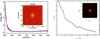 |
Fig. 1 High-resolution imaging of TOI-2095. Left panel: Keck NIR AO imaging and sensitivity curve for TOI-2095 taken in the Br-γ filter. The image reaches a contrast of ~7.4 magnitudes fainter than the host star within 0.″5. Inset: image of the central portion of the data. Right panel: speckle sensitivity curve of TOI-2095 taken with the SPeckle Polarimeter (SPP) at the Caucasian Observatory of Sternberg Astronomical Institute (SAI). Inset: speckle autocorrelation function. |
3.1.4 MuSCAT3 transit photometry
A transit event of TOI-2095b was observed with the Multicolor Simultaneous Camera for studying Atmospheres of Transiting exoplanets (MuSCAT3) instrument (Narita et al. 2020) mounted at the 2 m Faulkes Telescope North (FTN) at Haleakala Observatory on Maui, Hawai’i, USA. The instrument has a 9.1′ × 9.1′ field of view (0.27″ pixel−1 scale) and is capable of taking simultaneous images in the Sloan filters g′, r′, i′, and z′s. On the night of 29 May 2021 a transit of TOI-2095b was observed using all the MuSCAT3 filters, the exposure times were set to 15 s, 35 s, 30 s, and 20 s for g′, r′, i′, and z′s, respectively. The raw science images were calibrated with BANZAI and we performed aperture photometry using a custom MuSCAT3 pipeline. Although the transit event could not be detected with a significant degree of certainty, the data were useful to rule out EBs inside TESS pixel (Fig. B.2).
3.2 High-resolution imaging
3.2.1 Near-infrared adaptive optics imaging
Observations of TOI-2095 were taken by the NIRC2 instrument on Keck II telescope (Wizinowich et al. 2000) in the narrowangle mode with a full field of view of ~10″ and a pixel scale of approximately 0.0099442″ per pixel, on 9 September 2020 in the standard three-point dither pattern. The dither pattern step size was 3 and was repeated twice, with each dither having an offset from the previous dither by 0.5″. Observations were taken with the narrow band K filter (λ0 = 2.196; Δλ = 0.336 μm) with an exposure time of 0.181 s.
The sensitivities of the final combined adaptive optics image were determined by azimuthally injecting simulated sources around the primary target every 20° at separations of integer multiples of the central source’s full width at half maximum (FWHM; Furlan et al. 2017). The final sensitivity curve is shown in Fig. 1 (left panel). No close-in (≲ 1″) stellar companions were detected within the sensitivity limits.
3.2.2 Optical speckle imaging
TOI-2095 was observed in Ic band on 26 December 2020 UT with the SPeckle Polarimeter (SPP; Safonov et al. 2017) on the 2.5 m telescope at the Caucasian Observatory of Sternberg Astronomical Institute (SAI) of Lomonosov Moscow State University. As its detector, SPP uses an electron-multiplying CCD named Andor iXon 897. The detector has a pixel scale of 0.0206″ pixel−1 and a field of view of 5″ × 5″ centered on the star, and the angular resolution was 0.089″. The power spectrum was estimated from 4000 frames with 30 ms exposure. No stellar companions brighter than ΔIc = 3.0 mag and 6.4 mag at 0.2″ and 1.0″, respectively, were detected. The obtained sensitivity curve is shown in Fig. 1 (right panel).
3.2.3 Gaia assessment
We used Gaia DR3 data (Gaia Collaboration 2023) in order to complement our high-resolution imaging by searching for possible contaminating background, foreground, or bound stars inside or surrounding the SPOC photometric aperture. To do so, we used the tpfplotter package (Aller et al. 2020), which plots the nearby Gaia DR3 stars over the TESS target pixel files. In Fig. A.1, we show the tpfplotter outcome for each sector. There are two faint stars that fall inside several SPOC photometric apertures: Gaia DR3 2268372103913342080 (star #2, G = 20.4) and Gaia DR3 2268372477573039744 (star #3, G = 20.1). Having a magnitude difference of ΔG ~ 8 mag with TOI-2095 in both the Gaia and TESS bandpasses, each star dilutes the transit depth by a factor of ~6 × 10⁻⁴, which ensures that none of those stars can be the origin of the transit-like signal. Although negligible in practice, these dilutions are taken into account by the SPOC pipeline, which estimates an overall contamination ratio of ~1.08 × 10⁻³. We also checked the parallaxes and proper motions of the TOI-2095 nearby stars in order to identify possible bound members of the system, without finding matches (see also Mugrauer & Michel 2020, 2021).
Additionally, the Gaia DR3 astrometry provides information on the possibility of inner companions that may have gone undetected by either Gaia or the high-resolution imaging. The Gaia renormalised unit weight error (RUWE) is a metric whereby values that are ≲ 1.4 indicate that the Gaia astrometric solution is consistent with the star being single, whereas RUWE values ≳ 1.4 may indicate an astrometric excess noise, possibly caused by the presence of an unseen companion (e.g., Ziegler et al. 2020). TOI-2095 has a Gaia DR3 RUWE value of 1.13, meaning that the astrometric fit is consistent with a single star model.
3.3 CARMENES radial velocity monitoring
TOI-2095 was observed by the CARMENES spectrograph at the 3.5 m telescope at the Calar Alto Observatory in Almeria, Spain, as part of a follow-up program of TESS candidates for validation (22B-3.5-006; PI: E. Pallé). CARMENES has two channels: the visible one (VIS), which covers the spectral range 0.52–0.96 μm and the near-infrared one (NIR), which covers 0.96–1.71 μm; with an average spectral resolution for both channels of R = 94 600 and R = 80 400, respectively (Quirrenbach et al. 2014, 2018).
The star was observed by CARMENES from 1 April 2021 until 7 November 2021, collecting a total of 44 spectra with a time baseline of 219 days. The exposure time used to acquired the radial velocities (RVs) was of 1800 s. The data reduction was done with the CARACAL pipeline (Caballero et al. 2016b). CARACAL performs basic data reduction (bias, flat, and cosmic ray corrections) and extracts the spectra using the FOX optimal extraction algorithm (Zechmeister et al. 2014). The wavelength calibration is done following the algorithms described by Bauer et al. (2015). The RV measurements were computed with SERVAL3 (Zechmeister et al. 2018). SERVAL produces a template spectrum by co-adding and shifting the observed spectra and computes the RV shift relative to this template using a χ2 minimization with the RV shift as a free parameter. The RV measurements were corrected for barycentric motion, secular acceleration, instrumental drifts, and nightly zero points (for details see, e.g., Trifonov et al. 2018; Luque et al. 2018).
SERVAL also computes several activity indices, such as spectral line indices (Na I doublet λλ589.0nm, 589.6nm; Hα λ656.2 nm; and the Ca II infrared triplet λλλ849.8 nm, 854.2 nm, 866.2 nm), and other indicators such as the RV chromatic index (CRX) and the differential line width (dLW). These indicators are useful to monitor the stellar activity of the star and its effect on the RV measurements (cf. Zechmeister et al. 2018). Additionally we computed the activity indices from the cross-correlation function (CCF) using the raccoon4 pipeline (Lafarga et al. 2020). Raccoon uses weighted binary masks to compute the CCF and obtains RVs and the associated CCF activity indicators: FWHM, contrast (CON), and bisector (BIS).
The median overall signal-to-noise ratio (S/N) for the spectra taken with the visible channel was 297 with a standard deviation of 74 (minimum S/N = 79, maximum S/N = 394); for the near-infrared spectra the median S/N was 338 with a standard deviation of 104 (min. S/N = 84, max. S/N = 469). The median uncertainty values of the measured RVs were of 3.5 m s−1 (σdev = 1.5 m s−1) for the VIS channel and 11.7 m s−1 (σdev = 7.3m s−1) for the NIR channel. The visible and near-infrared SERVAL RV measurements are shown in Fig. C.1. In this work we used the RV data extracted using the visible channel, as this data set presented a lower scatter than the near infrared measurements. Extensive comparisons of the CARMENES VIS and NIR channel RVs have been provided elsewhere, especially by Reiners et al. (2018) and Bauer et al. (2020). The RV and activity indicators measured with SERVAL can be found in the Appendix (Tables C.1 and C.2) and the CCF activity indicators are given in Table C.3.
4 Stellar properties
4.1 Stellar parameters
Table 1 presents the coordinates, photometric and astrometric properties, and stellar parameters of TOI-2095. Throughout the text we use the TESS Object of Interest nomenclature, but the star was discovered almost 20yr ago by Lépine & Shara (2005) in the Digitized Sky Surveys because of its high proper motion. Afterwards, the star has been tabulated in a number of catalogs of relatively bright M dwarfs and potential targets for habitable planet surveys (e.g., Lépine & Gaidos 2011; Frith et al. 2013; Kaltenegger et al. 2019; Stelzer et al. 2022). We derived the effective temperature (Teff), surface gravity (log g), and iron abundance ([Fe/H]) of TOI-2095 with the SteParSyn5 code (Tabernero et al. 2022) using the line list and model grid described by Marfil et al. (2021). The line list of Marfil et al. (2021) makes use of both visible and near-infrared wavelength ranges available in CARMENES data. To obtain a conservative error estimate we used the systematic offset to interferometric effective temperatures of 72 K given by Marfil et al. (2021) as our systematic error, and added this to the measured stellar effective temperature uncertainty of 15 K. We estimated the target’s spectral type with ±0.5 dex accuracy from the colour-, absolute magnitude-, and luminosity-spectral type relations of Cifuentes et al. (2020). The stellar luminosity (L) was computed following Cifuentes et al. (2020) and the stellar mass (M*) and radius (R*) were determined following Schweitzer et al. (2019). We found TOI-2095 to be an M dwarf with Teff = 3759 ± 87 K, and a stellar mass and radius of M* = 0.44 ± 0.02 M⊙ and R* = 0.44 ± 0.02 R⊙, respectively.
We used the astrometric properties and RV measurements of TOI-2095 from Gaia DR3 (Gaia Collaboration 2023) to compute the galactocentric velocities (U, V, W) of the star following Cortés Contreras (2017). The velocities, presented in Table 1, were computed using a right-handed system and not corrected by the solar motion. The derived galactic velocities indicate that TOI-2095 belongs to the thin disk (Montes et al. 2001), suggesting an age > 1 Gyr. According to BANYAN Σ6 (Gagné et al. 2018), the U, V, W values indicate that TOI-2095 is not associated to any young moving group, supporting a relatively old age for this star.
Our derived iron abundance for TOI-2095 is [Fe/H] = −0.24 ± 0.04 dex. This value is in agreement to what is found for local stars, although TOI-2095 seems to be in the metal poor end compared to the median iron abundances of the Solar neighborhood. Casagrande et al. (2011) found a metallicity distribution function (MDF) slightly subsolar with a median [Fe/H] ~ −0.05 dex, but the same work pointed out that other studies found an MDF peak in the −0.2 to −0.1 dex range. For M stars, there have been studies pointing to an MDF with median values close to solar metaillicity (e.g., Bonfils et al. 2005; Casagrande et al. 2008), although planet-hosting M dwarfs typically appear to be metal-rich (e.g., Rojas-Ayala et al. 2010; Terrien et al. 2012; Hobson et al. 2018; Passegger et al. 2018).
Stellar parameters of TOI-2095.
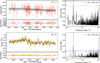 |
Fig. 2 Long-term photometric follow-up of TOI-2095 from ZTF (z band) and TJO (R band). Left panels: photometric time-series and joint best fitted model computed using GP adopting a quasi-periodic kernel (black line). The 1σ uncertainty regions of the fit are shown in light blue. The residuals of the fit are shown at the bottom panels. Right panels: GLS periodogram (Zechmeister & Kürster 2009) for each photometric data set. The vertical green line shows the fitted rotational period of the star. The horizontal lines represent the FAP levels of 10% (red dotted line) and 1% (blue dashed line). |
4.2 Stellar rotation from seeing-limited photometry
To obtain the rotation period of TOI-2095, we analyzed the photometric time series taken with ZTF (z band) and TJO (R band). We modeled the photometry using a linear function and a periodic term using Gaussian Processes (GP). To model the photometric variations, we used the GP package george (Ambikasaran et al. 2015) and chose a quasi-periodic kernel of the form:
![Mathematical equation: ${k_{ij\,{\rm{QP}}}} = A\,{\rm{exp}}\,\left[ {{{ - {{\left( {\left| {{t_i} - {t_j}} \right|} \right)}^2}} \over {2{l^2}}} - {{\rm{\Gamma }}^2}\,{{\sin }^2}\,\left( {{{\pi \left| {{t_i} - {t_j}} \right|} \over {{P_{{\rm{rot}}}}}}} \right)} \right],$](/articles/aa/full_html/2023/09/aa46692-23/aa46692-23-eq3.png) (1)
(1)
where |ti – tj| is the difference between two epochs or observations, the parameters A, l, and Γ are constants, and Prot is the period of the sinusoidal variation (i.e. the rotational period of a star).
For each photometric time series, we set as free parameters the two terms of the linear function and the constants describing the shape of the kernel from Eq. (1), while imposing Prot as a common term for both time series. We started the fitting procedure by optimizing a posterior probability function using PyDE7 and we used the optimal set of parameters to start exploring the parameter space using emcee (Foreman-Mackey et al. 2013).
Figure 2 shows the photometric time series from ZTF and TJO and their respective periodograms; the black line represents the model produced using the median of the posterior distributions of the fitted parameters and the blue shaded area the 1σ uncertainty of the model. The periodograms presented in this work were computed using the Generalized Lomb-Scargle (GLS) periodogram implementation by Zechmeister & Kürster (2009). We used a Python implementation of GLS8 that includes a subroutine to compute the false alarm probability (FAP) levels. This subroutine computes the FAP levels analytically using Eq. (24) of Zechmeister & Kürster (2009).
The root mean square of the residuals of the fit are rmsztf = 0.014 mag for ZTF and rmstjo = 0.004 mag for the TJO data. From the time series and periodograms, ZTF-z data present a larger scatter compared to TJO-R ones and there is no clear detection of a periodic signal in the photometry for the former data set. On the other hand, the periodogram for the TJO observations presents a significant peak around 40 days. An individual fit for both data sets using the previously described kernel resulted in a bimodal posterior distribution for ZTF with peaks around Prot ~ 40 and ~80 days, while the TJO fit delivered a rotation period of  days. Using our joint fit, we found a rotational period of
  days for TOI-2095, which will be our final adopted value. Based on the gyrochronology relations from open clusters, an early-M dwarf with a rotation period of 40 days is consistent with typical old field dwarf with ages of a few Gyr (Curtis et al. 2020). Based on these relations we conclude that TOI-2095 is likely older than the age of Praesepe (670 Myr old).
5 Analysis and results
5.1 Radial velocity and activity indices periodogram analysis
To search for the periodic variations in the RV of the star induced by the two transiting planet candidates, we computed the GLS periodogram. Figure 3 shows the periodograms for the CARMENES RV measurements (visible channel) and the activity indices provided by SERVAL. We marked the orbital periods of the two planet candidates using TESS ExoFOP ephemeris, the TOI-2095b period is represented by the orange vertical line, while TOI-2095c is highlighted by the blue vertical line. The measured rotation period based on ground-based photometric monitoring of the star is marked by the brown vertical line.
From Fig. 3 we note that several activity indices present a peak around P ~ 40 days, in agreement with the measured rotation period derived from ground-based photometric observations. The RV periodogram shows no evidence of significant peaks around the periods of the transiting candidates detected by TESS nor at the rotation period of the star. As a test, we removed the ~40 day rotation period from the RVs by fitting the data using a quasi-periodic kernel to model the stellar variability with a normal prior based on our derived value for the rotation period of the star. However, the power peaks at the expected orbital periods of the planets did not become significant in the periodogram. The non-detection of both transiting planets in the RV measurements is expected since the predicted RV amplitude for both planets is around ~0.9 m s−19, close to the precision limit of current spectrographs. However, reaching near 1 m s−1 RV precision with CARMENES is possible. For example, Kossakowski et al. (2023) detected an Earth-mass planet with a period of 15.6 days around the M dwarf Wolf 1069b. The induced RV semi-amplitude of this planet is 1.07 ± 0.17 m s−1. This detection was possible due to the large number of observation (262 RV measurements, close to 4 yr of baseline) and the low levels of activity of the star. With our RV data (44 measurements) and the stellar activity variability in the observations, we can only use the RV measurements to put upper limits on the masses of the transiting objects to validate them as planets.
5.2 TESS and CARMENES joint fit
We used the available TESS photometry and CARMENES RV measurements to perform a joint fit of the data. We decided to use TESS transit observations since the ground-based data presented only tentative transit detections of the transit events. We followed the method outlined in Murgas et al. (2021), which we briefly describe here. The transits of both planets were modeled using PyTransit10 (Parviainen 2015), we adopted a quadratic limb darkening (LD) law and used LDTK11 (Parviainen & Aigrain 2015) to compare the fitted LD coefficients with the expected values (based on the stellar parameters presented in Table 1). To model the planet-induced RV variations, we used RadVel12 (Fulton et al. 2018). The RV measurements were affected by the activity of the star and presented a moderate correlation with some of the stellar activity indices measured with SERVAL. In our case the activity index that presented the strongest correlation with the RVs was the Ca II IRT line, with a Pearson’s r = 0.46 (i.e., moderate correlation; see Figs. D.1 and D.2 for the correlation for the other activity indices). To account for this correlation, we fit a linear function using the Ca II IRT index as an independent variable and corrected the RV values using the fitted linear trend before performing the joint fit. With this approach, the stellar variability contribution (or part of) is taken into account and not modeled as a red-noise component only.
As a test, we fit the RV data using non-circular orbits for both planets and imposing normal priors in the orbital period and central time of the transits, using the values found by TESS while modeling the systemaic noise with GPs. We found that the orbital eccentricity (e) and argument of the periastron (ω) were unconstrained by the RV measurements, hence, we decided to adopt circular orbits for both planet candidates for the joint fit. The free parameters used in our modeling were the planet-to-star radius ratio Rp/R*, the quadratic LD coefficients, q1 and q2 (using Kipping 2013), the central time of the transit, Tc, the planetary orbital period, P, the stellar density, ρ*, the transit impact parameter, b, the RV semi-amplitude, KRV, the host star systemic velocity, γ, and the RV jitter (σRV jitter). We modeled the TESS correlated noise through a GP with a Matérn 3/2 kernel. This kernel has covariance properties that make it very appropriate to model TESS data in which the photometric variability is barely influenced by the stellar rotation and, instead, residual short-term red-noise structures dominate the correlated noise (Stefánsson et al. 2020; Castro-González et al. 2023). In the case of TOI-2095, we ran the GLS periodogram over the individual and joint TESS sectors and found no significant periodicities. Since those structures can vary from one sector to another, we modeled them with different Matérn 3/2 kernels, each of them taking the form:
 (2)
(2)
where |ti – tj| is the time between epochs in the series, and the hyperparameters, ck and τk, were allowed to be free, with k indicating the TESS sector.
For the RV measurements we modeled the stellar variability using an exponential squared kernel (i.e., a Gaussian kernel)
 (3)
(3)
where ti – tj is the time between epochs in the series, and the hyperparameters, crv and τrv, were set free.
We fit a total of 61 free parameters to model the photometric and RV measurements considering systematic noise. The fitting procedure started with the optimization of a joint posterior probability function with PyDE. We used the results of the optimization to start a Markov chain Monte Carlo (MCMC) procedure using emcee (Foreman-Mackey et al. 2013). We ran the MCMC using 250 chains for 15 000 iterations as a burn-in stage to ensure the convergence of the parameters, and then ran the main MCMC for another 16000 iterations. We computed the final values of our fitted parameters using the median and 1σ limits of the posterior distributions.
The fitted and derived parameters values can be found in Table 2 (see Fig. D.3 for the posterior distribution correlation plot of the parameters). The phase folded and systematic-free transit model and data are shown in Fig. 4, the individual TESS photometry and transit model including red noise is shown in Fig. D.4. Figure 5 presents the CARMENES RV measurements and the RV model of the data using the results of the joint fit.
From the analysis of all available data on TOI-2095, we find that both planets have similar sizes, with Rb = 1.25 ± 0.07 R⊕ for TOI-2095b and Rc = 1.33 ± 0.08 R⊕ for TOI-2095c. Due to their relatively long orbital periods (Pb = 17.665 days and Pc = 28.172 days) and the small RV amplitude induced by the transiting planets, we do not find significant evidence of the presence of the planets in our RV data. Additionally, the stellar activity of the star dominates the RV variations. We computed the mass upper limits using the RV equation from Cumming et al. (1999, and we refer to Perryman 2011 for a complete derivation) assuming M* ≫ Mp and e = 0. We set M* = 0.44 M⊙ and used the posterior distributions of the orbital period, orbital inclination, and RV amplitudes from the joint fit. The final upper limits were computed using the 95% percentile limit of the distribution of masses. Using this procedure, we found upper mass limits of Mb < 4.1 M⊕ and Mc < 7.4 M⊕ for TOI-2095b and TOI-2095c (see Figs. 5 and 6), respectively. However, these upper mass limits place both transiting candidates well into the planetary mass regime.
We checked whether we could detect any transit timing variations (TTVs) using TESS photometric data. We fit the transits with PyTTV (Korth et al., in prep.), allowing each central transit time to be free (values and 1σ uncertainties presented in Tables D.1 and D.2). Unfortunately, the individual transit events of both planets are too shallow to constrain the central times with the precision needed to detect TTVs − if they do, in fact, exist in this system (see Fig. 7).
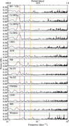 |
Fig. 3 GLS periodograms of the CARMENES RV measurements taken with the optical channel, spectral activity indices, and window function. The horizontal lines represent the false alarm probability (FAP) levels of 10% (red dotted line) and 1% (green dash line). The vertical lines mark the period of planets TOI-2095b (P = 17.66 days, solid orange line), TOI-2095c (P = 28.17 days, solid blue line), and the measured rotation period of the star from photometric observations (P = 40 days: dashed brown line). |
5.3 Statistical validation
We also performed a statistical validation analysis for TOI-2095b and TOI-2095c based on TESS photometry, CARMENES spectroscopy, Keck NIR AO imaging, and SPP optical speckle imaging. To do so, we used the vespa package (Morton 2012, 2015) to compute false positive probabilities (FPPs), that is, the probabilities of planet candidates being astrophysical false positives: eclipsing binaries (EBs), background (or foreground) EBs blended with the target star (BEBs), or hierarchical triple systems (HEBs). The most commonly adopted threshold to consider a candidate as statistically validated planet is to have a FPP lower than 1% (FPP < 0.01; e.g., Rowe et al. 2014; Montet et al. 2015; Castro Gonzalez et al. 2020; de Leon et al. 2021; Christiansen et al. 2022). However, relying on the FPP alone can lead to mis-classifications (Livingston et al. 2018; Mayo et al. 2018). Hence, before assigning the candidate disposition, we checked that our system meets the following conditions: transit S/N > 10, odd-even mismatch of transit depths < 3σ, Gaia RUWE ≲ 1.4, and the absence of contaminant sources within the photometric aperture (Sect. 3.2.3). The latter condition has been shown to be of crucial importance, since the re-analysis of early validation works in which it had not been taken into account led to the deprecation of several validated planets such as K2-78b, K2-82b, K2-92b (Cabrera et al. 2017), and K2-120b (Castro-Gonzalez et al. 2022).
In the following, we describe the information supplied to vespa for the statistical validation analysis of TOI-2095b and TOI-2095c. We input the target coordinates and parallax from Gaia DR3 (Gaia Collaboration 2023), HJK photometry from 2MASS (Skrutskie et al. 2006), and the CARMENES spectroscopic parameters Teff, [Fe/H], and log g (Table 1). We also supplied the orbital periods and planet-to-star radius ratios from our fit (Table 2). We constrained the maximum allowed depth for a secondary eclipse to be thrice the standard deviation of the out-of-transit region of the TESS light curve. We also constrained the maximum aperture radius from which the signal is expected to come from by circularizing the largest SPOC aperture as  following Castro-González et al. (2022), being A the maximum aperture area. Finally, we input the TESS light curve folded to the candidate period as well as the Keck and SPP contrast curves, which significantly decrease the FPP by discarding the presence of stars above certain brightness at a certain projected distance.
In Table 3, we show the vespa posterior probabilities for TOI-2095b and TOI-2095c. In both cases, the FPP is lower than 1 %, so both planets are independently validated. Moreover, planet candidates located in multi-transiting systems are more likely to be genuine planets than those in single planet candidate systems (Latham et al. 2011; Lissauer et al. 2011). Hence, we followed the statistical framework introduced by Lissauer et al. (2012) in order to compute the multiplicity-corrected FPP as FPP2 = 1 – P2, that is,
 (4)
(4)
where P1 = 1 − FPP and X2 is the “multiplicity boost” for systems with two planet candidates. Similar to Guerrero et al. (2021), we compute for the TESS postage stamps a X2 of 44 for two-planet systems with small planet candidates (R < 6 R⊕). As a result, we obtain multiplicity-corrected FPPs of FPP2,b = 3.54 × 10⁻⁶ and FPP2,c = 3.14 × 10⁻⁵, which supports the planetary nature of TOI-2095b and TOI-2095c.
Fitted and derived parameters of TOI-2095b and TOI-2095c.
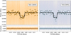 |
Fig. 4 TESS phase-folded light curves after subtracting the photometric variability for TOI-2095b (top left) and TOI-2095c (top right). The best-fit model is shown in black, the circles are TESS binned data points, and the points are individual TESS observations. Bottom panels: residuals of the fit. |
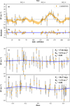 |
Fig. 5 Radial velocity measurements of TOI-2095 taken with CARMENES. (a): RV time series and best-fitting model (blue line) including red noise. The plotted RV model was computed using the median values of the posterior distribution for each fitted parameter. The shaded area around the blue line represent the 1σ uncertainty levels of the fitted model. (b): residuals of the fit after subtracting the two planet models. (c) and (d): phase-folded RV measurements after subtracting the red noise and best-fit model (blue line). |
Posterior probabilities for the EB, BEB, HEB, and planet scenarios for TOI-2095b and TOI-2095c as computed with vespa.
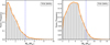 |
Fig. 6 Posterior distributions for the planetary masses of TOI-2095b and TOI-2095c. The vertical dashed blue line represents the 95% confidence limit for each planet; for TOI-2095b, we And a mass upper limit of Mb < 4.1 Μ⊕ and for TOI-2095c, it is Mc < 7.4 M⊕. |
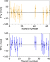 |
Fig. 7 Central mid-transit times measured using TESS data for TOI-2095b (top panel) and TOI-2095c (bottom panel). The shaded areas represent the 1σ and 3σ uncertainty limits for the central time of the transit measurements. |
6 Planet searches and detection limits from the TESS photometry
Besides the two planets found by SPOC orbiting TOI-2095, we wondered if extra transiting planets might exist in the system and remain unnoticed. To this end, we searched for hints of new planetary candidates using the SHERLOCK13 pipeline (see, e.g., Pozuelos et al. 2020; Demory et al. 2020).
SHERLOCK allows for the exploration of TESS data to recover known planets, candidates and to search for new signals that might be attributable to planets. The pipeline combines different modules to (1) download and prepare the light curves from their repositories, (2) search for planetary candidates using the tls algorithm (Hippke & Heller 2019), (3) perform an in-depth vetting of interesting candidates to rule out any potential systematic origin of the detected signals, (4) conduct a statistical validation using the TRICERATOPS package (Giacalone et al. 2021), (5) model the signals to refine their ephemerides through the allesfitter code (Günther & Daylan 2021), and (6) compute observational windows from user-specific ground-based observatories to trigger a follow-up campaign.
The transit search is optimized by removing any undesired trends in the data, such as instrumental drifts, implementing a multi-detrend approach by means of the wotan package (Hippke et al. 2019). This strategy consists of detrending the nominal PDCSAP light curve several times using a biweight filter by varying the window size. In our case, we performed 20 detrendings with window sizes ranging from 0.20 to 1.30 days.
Then, SHERLOCK simultaneously conducts the transit search in each new detrended light curve jointly with the nominal PDC-SAP flux. Once the transit search is done, SHERLOCK combines all the results to choose the most promising signal to be a planetary candidate. This selection is performed considering many aspects, such as the detrend dependency of a given signal, the S/N, the signal-detection-efficiency (SDE), and the number of times that a given signal is happing in borders, among others.
The entire search process follows a search-find-mask loop until no more signals are found above user-defined S/N and SDE thresholds; that is, once a signal is found, it is stored and masked, and then the search continues. Due to the number of sectors available for TOI-2095, we split our search into two independent blocks: first, considering all the sectors observed during the primary mission, that is, Sectors 14, 15, 16, 17, 18, 19, 20, 21, 22, 23, 24, and 26; secondly, the sectors observed during the extended mission, that is, 40, 41, 47, 48, 49, 50, 51, 52, 53, 54, and 55. The motivation to follow this strategy is twofold: on the one hand, the larger the number of sectors we inspect, the higher the computational cost. On the other hand, any actual planetary signal should be recovered independently in both experiments; otherwise, the credibility of the detected signal is lower, hinting that the real source of the signal might be related to some instrumental issues.
We focused our search on orbital periods ranging from 0.5 to 60 days, where a minimum of two transits was required to claim a detection. We recovered the TOI-2095.01 and .02 signals in the first and second runs, respectively. In the subsequent runs, we did not find any other signal that hinted at the existence of extra transiting planets. We found other signals, but they were too weak to be considered planetary candidates or were attributable to variability, noise, or systematics. Hence, our search for extra planets yielded negative results, confirming only the two detections reported by SPOC.
As asserted in previous studies (see, e.g., Wells et al. 2021; Schanche et al. 2022; Delrez et al. 2022), the lack of extra signals might be due to one of the following scenarios: (1) no other planets exist in the system; (2) they do exist, but they do not transit; (3) they do exist and transit but have orbital periods longer than the ones explored during our search process; or (4) they do exist and transit, but the photometric precision of the data is not accurate enough to detect them.
Scenarios (1) and (2) might be further explored by conducting an intense RV follow-up campaign. Unfortunately, with our current RV data described in Sect. 5.1, we cannot constrain if other smaller or longer-orbital period planets are present in the system. Scenario (3) can be tested by adding a more extended time baseline, for example, using the data from Sectors 56, 57, 58, 59, and 60. However, accumulating new sectors would not significantly increase our detection capability due to the already large data set used in this study. Finally, to evaluate scenario (4), we studied the detection limits of the TESS photometry performing injection-and-recovery experiments with the MATRIX code14 (Dévora-Pajares & Pozuelos 2022).
MATRIX allows the user to inject synthetic planets over the PDCSAP light curve and perform a transit search following a similar strategy to SHERLOCK. In this study, due to the relatively long orbital periods of both planets, ~ 17.6 days for planet b and ~28.2 days for planet c, there is an extensive range of orbital periods where a small innermost planet may orbit. Furthermore, assuming a nearly coplanar configuration for planetary orbits, the transit probability for any hypothetical inner planet would be higher than for planets beyond planet c. For this reason, we focused our injection-and-recovery experiment on planets with orbital periods shorter than planet b; that is, we explored the Rplanet–Pplanet parameter space in the ranges of 0.5–3.0 R⊕ with steps of 0.28 R⊕, and 0.5–16.0 days with steps of 0.26 days.
For each combination of Rplanet–Pplanet, MATRIX explores five phases, that is, different values of T0. Then, in total we explored 3000 scenarios. For simplicity, the injected planets have eccentricities and impact parameters equal to zero. Once the synthetic planets are injected, MATRIX detrends the light curves using a bi-weight filter with a window size of 0.75 day, which was found to be optimal during the SHERLOCK search and masked the transits corresponding to TOI-2095b, and c. A synthetic planet is recovered when its epoch matches the injected epoch with 1 h accuracy, and its period is within 5 % of the injected period.
The results obtained during these injection-and-recovery experiments are displayed in Fig. 8. We found that Earth- and sub-Earth size planets would remain unnoticed almost for the complete set of periods explored. However, planets with sizes larger than Earth seem to be easy to find, with recovery rates > 80%. Hence, we can rule out the presence of inner transiting planets to TOI-2095b with sizes > 1 R⊕.
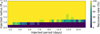 |
Fig. 8 Injection-and-recovery experiment performed to test the detectability of inner planets in the system using the TESS sectors described in Sect. 2. We explored a total of 3000 different scenarios. Each pixel evaluated about eight scenarios, that is, eight light curves with injected planets having different Pplanet, Rplanet, and T0. Higher recovery rates are presented in yellow and green colors, while lower recovery rates are shown in blue and darker hues. Planets smaller than 1.0 R⊕ would remain undetected for the explored periods. |
7 Dynamical analysis
7.1 Stability-constrained characterization
The current data on the TOI-2095 system does not allow for strong constraints on the masses and eccentricities of the two super-Earths. We explored the possibility of obtaining tighter constraints on these parameters through dynamical stability considerations. Similar to many previous works (see, e.g., Jenkins et al. 2019; Demory et al. 2020; Pozuelos et al. 2020; Delrez et al. 2021, 2022), we made use of the Mean Exponential Growth factor of Nearby Orbits (MEGNO; Cincotta & Simó 2000; Cincotta et al. 2003) chaos indicator implemented within the REBOUND N-body integration software package (Rein & Liu 2012). We used the WHFast integration scheme (Rein & Tamayo 2015), an implementation of the Wisdom-Holman symplectic mapping algorithm (Wisdom & Holman 1991). The time-averaged MEGNO value, 〈Y(t)〉, resulting from an integration indicates the divergence of the planets’ trajectories after small perturbations of their initial conditions. For chaotic motion, 〈Y(t)〉 grows without bound as t → ∞, whereas for regular motion, 〈Y(t)〉 → 2 for t → ∞.
We constructed two sets of MEGNO stability maps to explore the dynamical behavior in the Mb – Mc and eb – ec parameter spaces. Based on the current constraints for the planetary masses (Fig. 6), we explored values ranging from 0–7 M⊕ for TOI-2095b and 0–12 M⊕ for TOI-2095c. As for the eccentricity map, we considered values ranging from 0–0.2 for both planets. We constructed 20 × 20 grids in the parameters for both the Mb – Mc and eb – ec MEGNO maps. For each grid cell, we randomly sampled ten different initial conditions for the mean anomalies and arguments of periastron, (M, ω ~ Unif [0°, 360°]). The values represented in each grid cell are the average of the 10 different initial conditions for M and ω. In the Mb – Mc map, we froze the values of all the other parameters, including eccentricity, to their nominal values. Similarly, when exploring the eccentricity space, we froze the values of all other parameters, including mass, to their nominal values. The integration time and timestep for each realization were set to 106 orbits of TOI-2095c and 5% of the orbital period of TOI-2095b, respectively.
After running the 4000 realizations for the Mb – Mc parameter space, we found that the system is fully stable through the entire range of masses studied. Therefore, we could not further constrain the masses of TOI-2095b and TOI-2095c using stability considerations. The eb – ec parameter space, on the other hand, reveals a much larger variation. With sufficiently large eccentricities for one or both planets, the MEGNO value indicates the system’s chaotic behavior (Fig. 9).
Similar to what was found by Demory et al. (2020), we determined three regions of differing stability: A (fully stable), B (transition region), C (fully unstable). When the system is fully stable (A), the eccentricities obey the following inequality:
 (5)
(5)
When the system is fully unstable (C), the eccentricities satisfy:
 (6)
(6)
The transition region falls between the lines indicated by the aforementioned inequalities.
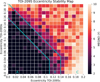 |
Fig. 9 Stability map of the TOI-2095 system in the eb – ec parameter space based on the MEGNO chaos indicator. The map consists of a 20 × 20 grid, where each grid cell is the average of 10 realizations with randomized mean anomalies and arguments of periastron. The three regions of differing stability (A, B, C) are marked with letters and are described by Eqs. (5) and (6). |
7.2 Constraints on potential additional planets
The TOI-2095 system may have additional planets other than planets b and c. Short-period super-Earths are often found in tightly-spaced, high-multiplicity systems, particularly around M dwarfs (e.g., Fabrycky et al. 2014; Dressing & Charbonneau 2015). Here, we explore the parameter space in which an additional third planet in the system could exist in stable orbits. We used the Stability Orbital Configuration Klassifier (SPOCK; Tamayo et al. 2020), which is a machine-learning model trained on ~100 000 orbital configurations of three-planet systems, to classify the long-term orbital stability of a given planetary system.
We considered two types of simulations for the TOI-2095 system with an injected third planet (“planet d”). In the first version, we assumed a circular orbit for planet d. To start, we also considered planets b and c to have circular orbits. We explored the ad – Md space of the additional planet within a 200 × 200 grid in which ad was varied from 0.01–0.3 au and Md was varied from 1–10 M⊕. Each grid cell represents the average of ten realizations of the system with randomized values of the inclinations, mean anomalies, and longitudes of ascending node (i - Rayleigh(1°), M, Ω ~ Unif [0°, 360°]). All other parameters in the system were set to their nominal values. The resulting parameter space map is shown in the top panel of Fig. 10. We note various bands of instability throughout a range of values of ad. There are negligible variations with the mass, Md. We also explored how these results change when the orbits of planets b and c are eccentric. We ran the same suite of simulations but randomly sampled the eccentricities of TOI-2095 b and c (e ~ Rayleigh(0.05)). We found a wider region of instability in the ad – Md space, along with small variations with the mass Md. Specifically, for Md = 1 M⊕, the band of instability has a width of ~0.085 au (0.075–0.16 au). On the other hand, when Md = 10 M⊕, it increases in width to ~0.12 au (0.065–0.185 au).
For the second type of simulations, we relaxed the assumption of a circular orbit for the hypothetical third planet and varied both its eccentricity and semi-major axis. Based on the results of the circular case, which showed negligible mass variations, we considered a fixed mass for planet d, md = 5 M⊕, and explored the ad – ed parameter space in a 200 × 200 grid in which ad was varied from 0.01–0.3 au and ed was varied from 0–0.3 (bottom panel of Fig. 10). Each pixel contains the average of 10 realizations of the system with randomized values for the inclinations, mean anomalies, and longitudes of ascending node (i ~ Rayleigh(1°), M, Ω ~ Unif[0°, 360°]). The map indicates that a wide swath of parameter space is disallowed depending on the eccentricity of planet d.
7.3 Propects for transit timing variations follow-up
Our best fit (described in Sect. 5.2) indicates that the resulting period ratio Pc/Pb is 1.595, placing the system within ~10% of the first-order 3:2 mean-motion resonance. In such a configuration, the gravitational pull exerted between the planets may lead to mutual orbital excitation, which induces measurable TTVs (Agol et al. 2005; Holman & Murray 2005). In Sect. 5.2, we describe our search for hints of these TTVs in the TESS data; unfortunately, we concluded that the low S/N of individual transits prevents us from finding any deviation from their linear prediction.
Hence, in this section, we explore the amenability of this system to be followed up by a dedicated observational campaign in the search for TTVs that allows for the planetary masses to be estimated. To this end, we conducted a detailed analysis of the expected TTVs amplitudes for TOI-2095b and c, following the strategy presented by Pozuelos et al. (2023).
This strategy consisted of generating 1000 synthetic configurations by drawing orbital periods and mid-transit times from the values reported in Table 2 and following normal distributions. We imported the planetary mass distributions from the posteriors found in the joint analysis (see Fig. 6). During our fitting process, for simplicity, we assumed circular orbits. However, some level of eccentricity might exist. Indeed, recent studies suggest a relationship connecting the number of planets in a given system and their eccentricities, where it has been found that the greater the number of planets, the lower the eccentricities (see, e.g., Limbach & Turner 2015; Zinzi & Turrini 2017; Zhu et al. 2018). For two-planet systems, the distribution of eccentricities follows a lognormal distribution with μ =−1.98 and σ = 0.67 (He et al. 2020). We drew the eccentricities for our synthetic systems from such a distribution, adding the additional constraint obtained in Sect. 7 that limits the mutual values by Eq. (5).
Moreover, we sampled the argument of periastron and the mean anomaly following a random distribution from 0 to 2π. Then, to compute the TTVs amplitude for each synthetic system, we used the TTVFast2Furious package (Hadden 2019). It is important to note that in this process, there is a non-null probability of obtaining unstable configurations due to drawing extreme values of masses and eccentricities simultaneously (not yet considered in Sect. 7). Then, to prevent considering unrealistic architectures in our analysis, we evaluated the stability of each scenario by computing the MEGNO parameter for an integration time of 105 orbits of the TOI-2095b, and took only those with Δ〈Y(t)〉= 2.0 − 〈Y(t)〉 < 0.1, which corresponded to ~92% of the drawn systems.
We found that the TTVs for each planet follow a nonsym-metric distribution, which we fit using the Skew-normal function from the scipy package (Virtanen et al. 2020). Following this procedure, we derived for each planet the probability density function (PDF) for the TTVs (see Fig. 11). On the one hand, we found for both planets that the modes of the PDF are in the subminute regime. On the other hand, the means of the PDFs are at ~3.1 and ~1.7 min, respectively. Hence, from these results, we concluded that measuring the planetary masses via TTVs is challenging and requires observations with mid-transit time precisions ≲1 min.
The best individual mid-transit time precision that we achieved using TESS for TOI-2095b and TOI-2095c are on the order of 5–7 min (Tables D.1 and D.2), thus making the detection TTVs with this satellite difficult. Another space mission dedicated to study transiting planets is the CHaracterising ExOPlanet Satellite (CHEOPS; Benz et al. 2021). Although its photometric measurements might be precise enough (< 20 s precision for G ~ 9 mag star, < 2 min for G ≥ 11 mag; Borsato et al. 2021), to our knowledge, CHEOPS has not yet observed TOI-2095. From the ground, the sub-millimagnitude transit depth of both planets make the detection of the transit with telescopes in the 1–2 m range challenging; it is likely that the transits would need to be observed with telescopes larger than 4m to detect the transits and have accurate mid-transit time precisions. A candidate for such observations would be the 10.4 m Gran Telescopio Canarias (GTC, Cepa et al. 2000) with its HiPERCAM instrument (Dhillon et al. 2021). This is an optical camera capable of taking simultaneous images in five Sloan bands: u, g, r, i, and z. This instrument has reached individual mid-transit precisions of less than a minute for a faint (V = 16.5 mag) TESS transit candidate (Parviainen et al., in prep.).
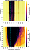 |
Fig. 10 Stability map of TOI-2095 for a hypothetical third planet in the system. Top panel: stability map for a third planet in a circular orbit case. Each cell of the 200 × 200 grid considers a different combination of ad and Md and represents the average value of 10 randomized realizations of the system’s initial conditions (i, ω, M). Bottom panel: stability map for a third planet in a eccentric orbit case. The map consists of 100 x 100 grid cells plotted in the ad – ed space. In both panels, the colorbar indicates the probability of stability from SPOCK (Tamayo et al. 2020). The vertical dashed lines denote the locations of TOI-2095b (cyan) and TOI-2095c (green). |
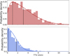 |
Fig. 11 Expected TTVs amplitudes for planets TOI-2095b (upper panel) and TOI-2095c (lower panel). Dashed and solid vertical lines correspond to the mode and the mean of the PDF, respectively. |
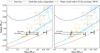 |
Fig. 12 Mass-radius diagramofall known transiting exoplanets taken from TepCat(Southworth 2011). Theupperlimits forthe masses of TOI-2095b and TOI-2095c derived from RV measurements (Mb < 4.1 M⊕ and Mc < 7.4 M⊕ respectively) are delimited by the black arrows. The predicted masses and uncertainties for TOI-2095b and TOI-2095c computed with the mass-radius relations of Chen & Kipping (2017, left) and Kanodia et al. (2019, right) are marked by the yellow and light blue star respectively. We show planets with P < 30 days and with mass determinations with an uncertainty better than 30%. Planets around stars with Teff ≤ 4000 K and Teff > 4000 K are marked by orange circles and blue triangles, respectively. The lines represent the composition models of Zeng et al. (2016, 2019) for pure iron cores (100% Fe, brown solid line), Earth-like rocky compositions (32.5% Fe plus 67.5% MgSiO3, dash green line), and a water world (0.1% H2 envelope plus 49.95% Earth-like rocky core plus 49.95% H2O, dash-dotted blue line). |
8 Discussion
TOI-2095b and TOI-2095c are a new addition to the growing list of transiting planets orbiting around M dwarfs. We derived the radii and upper mass limits for both planets (Rb = 1.25 ± 0.07 R⊕, Mb < 4.1 M⊕; Rc = 1.33 ± 0.08 R⊕, Mc < 7.4 M⊕) and estimated their equilibrium temperatures (Teq b = 347 ± 9 K, Teq c = 297 ± 8 K; assuming an Earth-like Bond albedo of ABond = 0.3). Figure 12 presents amass-radius diagram of known transiting planets using data taken from TepCat (Southworth 2011) and the composition models of Zeng et al. (2016, 2019). The models assume an isothermal atmosphere with 300 K and are truncated at a pressure level of 1 millibar (defining the radius of the planet). TOI-2095b and TOI-2095c are also shown in the diagram using their derived radii and upper mass limits. However, without a more precise mass measurement, it is hard to assess the bulk composition of TOI-2095b and TOI-2095c.
To estimate the true masses of TOI-2095b and TOI-2095c, we used the mass-radius (M–R) relations of Chen & Kipping (2017) and Kanodia et al. (2019). Chen & Kipping (2017) M–R relation was computed using a probabilistic approach based on mass and radius measurements across the parameter space starting from dwarf planets to late-type stars; the Python implementation of their M–R relation, forecaster, is publicly available15. Kanodia et al. (2019) implement the nonparametric M-R relations of Ning et al. (2018), we use Kanodia et al. (2019) nonparametric M–R relation computed using the measurements of 24 exoplanets around M dwarfs. Kanodia et al. (2019) also provide a Python implementation of their M–R relation called MRExo16. To compute the masses of TOI-2095b and TOI-2095c with forecaster and MRExo we used as input the posterior distributions of the planet-to-star radius ratio multiplied by the stellar radius presented in Table 1. Using Chen & Kipping (2017) we find values of  and
and  for TOI-2095b and TOI-2095c, respectively. On the other hand, using Kanodia et al. (2019) we find lower median mass values of
  for TOI-2095b and
  for TOI-2095c. These values can only be regarded as indicative of the possible final masses.
Despite their relatively small predicted RV amplitude, current instruments may be able to detect both planets with a more intensive follow-up campaign. For example, Wolf 1069b (Kossakowski et al. 2023) was discovered using CARMENES. This planet has an orbital period of 15.6 days (placing it in the HZ of their star) and a measured RV semi-amplitude of K = 1.07 ± 0.17 m s−1 (Sect. 5.1). The ultra-short-period planet GJ 367b (Lam et al. 2021) was discovered using TESS and has a mass measurement using HARPS. The reported RV semiamplitude of this planet is K = 0.79 ± 0.11 m s−1. In the case of 8 m class telescopes, RV detections lower than the 1 m s−1 threshold has been achieved by ESPRESSO at the Very Large Telescope (Proxima Cen d candidate; Suárez Mascareño et al. 2020; Faria et al. 2022). The stellar activity of the host star may present a challenge for the RV detection, but the combined use of contemporaneous photometric observations to monitor the stellar variability and GPs has delivered some results for the mass measurements of young planets (e.g., Suárez Mascareño et al. 2021).
Luque & Pallé (2022) recently proposed that small planets around M dwarf hosts seem to fall into two categories: an Earthlike composition or water world with equal mass fraction of ices and silicates. Using the upper limits of the planet masses, both planets in the TOI-2095 system would be compatible with both compositions. However, no water worlds were identified by Luque & Pallé (2022) below 1.5 R⊕, which suggests that the planets may have an Earth-like composition.
Finally, Fig. 13 shows the instellation flux in Earth units versus effective temperature of the planet host star. The vertical lines represent the limits of the habitable zone (HZ) defined by Kopparapu et al. (2013). Both planets are on orbits that place them well within the runaway greenhouse limit, where planets having volatiles are expected to have atmospheres dominated by them until complete desiccation occurs (Ingersoll 1969; Kasting 1988). The question of how runaway greenhouse effects impact the volatile content and habitability of terrestrial-sized exoplanets is a subject of current research (e.g., Turbet et al. 2019; Mousis et al. 2020) and such atmospheric studies of planets within the runaway greenhouse region may provide valuable insights (Suissa et al. 2020). A different approach is to statistically investigate instellation-induced changes of bulk parameters such as planetary radius, whose magnitudes are predicted to exceed the resolution of state-of-the-art high precision photometry (Turbet et al. 2020; Dorn & Lichtenberg 2021). Planets close to the runaway greenhouse limit, such as TOI-2095b and TOI-2095c, are key in such attempts to empirically test the HZ hypothesis. This holds, in particular, if additional outer planets (whose existence we cannot test with the currently available data) allow us to probe planets on both sides of the instellation threshold within the same system (Turbet et al. 2019).
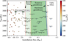 |
Fig. 13 Incident flux in Earth units versus stellar effective temperature for known exoplanets (data taken from NASA Exoplanet Archive). The color of each circle represents the equilibrium temperature of the planet. The habitable zone limits of Kopparapu et al. (2013) are shown with lines. The position of TOI-2095b and TOI-2095c are marked by the green stars. |
9 Conclusions
We report the validation of two transiting planets around the M dwarf TOI-2095 discovered by TESS. We use ground-based high-resolution imaging, TESS photometric data, and CARMENES RVs to discard false positive scenarios, measure the planetary radii, and place stringent upper limits on the masses of the transiting candidates.
The star is an M dwarf located at a distance d = 41.90 ± 0.03 pc and is relatively bright in the near-infrared (J = 9.8 mag, Ks = 8.9 mag). We derive an effective temperature of Teff = 3759 ± 87 K and an iron abundance of [Fe/H]= −0.24 ± 0.04 dex, as well as a stellar mass and radius of M = 0.44 ± 0.02 M⊙ and R = 0.44 ± 0.02 R⊙, respectively. Using ground-based photometric observations, we determined a stellar rotation period of  days, in agreement with the spectroscopic activity indices measured from CARMENES data.
In order to obtain the transit and orbital parameters of the system we fitted 22 sectors of TESS data and CARMENES RV measurements simultaneously, while taking into account the red noise present in both time series using Gaussian processes. We assumed circular orbits for both transiting planets. We find that the inner planet, TOI-2095b, has an orbital period of Pb = 17.665 days, a radius of Rb = 1.25 ± 0.07 R⊕, an upper mass limit of Mb < 4.1 Me, and an equilibrium temperature of Teq = 347 ± 9 K (assuming a Bond albedo of 0.3). The other transiting planet, TOI-2095c, has an orbital period of Pc = 28.172 days, a radius of Rc = 1.33 ± 0.08 R⊕, an upper mass limit of Mc < 7.4 M⊕, and an equilibrium temperature of Teq = 297 ± 8 K (assuming a Bond albedo of 0.3).
Both planets present interesting sizes and temperatures that makes them attractive targets for further follow-up observations. In particular, extremely precise RV follow-up observations can help to improve the mass measurements (and, hence, the bulk densities) of these planets and provide some constraints for future prospects for atmospheric characterizations.
Acknowledgements
We thank the anonymous referee for the constructive report. CARMENES is an instrument at the Centro Astronomico Hispano en Andalucia (CAHA) at Calar Alto (Almeria, Spain), operated jointly by the Junta de Andalucia and the Instituto de Astrofisica de Andalucia (CSIC). CARMENES was funded by the Max-Planck-Gesellschaft (MPG), the Consejo Superior de Investigaciones Cientificas (CSIC), the Ministerio de Economia y Competi-tividad (MINECO) and the European Regional Development Fund (ERDF) through projects FICTS-2011-02, ICTS-2017-07-CAHA-4, and CAHA16-CE-3978, and the members of the CARMENES Consortium (Max-Planck-Institut für Astronomie, Instituto de Astrofisica de Andalucia, Landessternwarte Königstuhl, Institut de Ciències de l’Espai, Institut für Astrophysik Göttingen, Universidad Complutense de Madrid, Thüringer Landessternwarte Tautenburg, Instituto de Astrofisica de Canarias, Hamburger Sternwarte, Centro de Astrobiologia and Centro Astronomico Hispano-Alemân), with additional contributions by the MINECO, the Deutsche Forschungsgemeinschaft through the Major Research Instrumentation Programme and Research Unit FOR2544 “Blue Planets around Red Stars”, the Klaus Tschira Stiftung, the states of Baden-Württemberg and Niedersachsen, and by the Junta de Andalucia. This paper includes data collected by the TESS mission, which are publicly available from the Mikulski Archive for Space Telescopes (MAST). Funding for the TESS mission is provided by NASA’s Science Mission directorate. Resources supporting this work were provided by the NASA High-End Computing (HEC) Program through the NASA Advanced Supercomputing (NAS) Division at Ames Research Center for the production of the SPOC data products. We acknowledge the use of public TESS data from pipelines at the TESS Science Office and at the TESS Science Processing Operations Center. This research has made use of the Exoplanet Follow-up Observation Program website, which is operated by the California Institute of Technology, under contract with the National Aeronautics and Space Administration under the Exoplanet Exploration Program. This work has made use of data from the European Space Agency (ESA) mission Gaia (https://www.cosmos.esa.int/gaia), processed by the Gaia Data Processing and Analysis Consortium (DPAC, https://www.cosmos.esa.int/web/gaia/dpac/consortium). Funding for the DPAC has been provided by national institutions, in particular the institutions participating in the Gaia Multilateral Agreement. This work makes use of observations from the LCOGT network. Part of the LCOGT telescope time was granted by NOIRLab through the Mid-Scale Innovations Program (MSIP). MSIP is funded by NSF. The Telescopi Joan Oro (TJO) of the Montsec Observatory (OdM) is owned by the Generalitat de Catalunya and operated by the Institute for Space Studies of Catalonia (IEEC). This paper is based on observations made with the MuSCAT3 instrument, developed by the Astrobiology Center and under financial supports by JSPS KAKENHI (JP18H05439) and JST PRESTO (JPMJPR1775), at Faulkes Telescope North on Maui, HI, operated by the Las Cumbres Observatory. Based on observations obtained with the Samuel Oschin 48-inch Telescope at the Palomar Observatory as part of the Zwicky Transient Facility project. ZTF is supported by the National Science Foundation under Grant No. AST-1440341 and a collaboration including Caltech, IPAC, the Weizmann Institute for Science, the Oskar Klein Center at Stockholm University, the University of Maryland, the University of Washington, Deutsches Elektronen-Synchrotron and Humboldt University, Los Alamos National Laboratories, the TANGO Consortium of Taiwan, the University of Wisconsin at Milwaukee, and Lawrence Berkeley National Laboratories. Operations are conducted by COO, IPAC, and UW. The results reported herein benefited from collaborations and/or information exchange within the program “Alien Earths” (supported by the National Aeronautics and Space Administration under agreement no. 80NSSC21K0593) for NASA’s Nexus for Exoplanet System Science (NExSS) research coordination network sponsored by NASA s Science Mission Directorate. This publication makes use of data products from the Wide-field Infrared Survey Explorer, which is a joint project of the University of California, Los Angeles, and the Jet Propulsion Laboratory/California Institute of Technology, funded by the National Aeronautics and Space Administration. We acknowledge financial support from the Agencia Estatal de Investigacion (AEI/10.13039/501100011033) of the Ministerio de Ciencia e Innovacion and the ERDF “A way of making Europe” through projects PID2021-125627OB-C31, PID2019-109522GB-C5[1:4], and the Centre of Excellence “Severo Ochoa” and “Maria de Maeztu” awards to the Instituto de Astrofisica de Canarias (CEX2019-000920-S), Instituto de Astrofisica de Andalucia (SEV-2017-0709) and Institut de Ciències de l Espai (CEX2020-001058-M). This work was also funded by the Generalitat de Catalunya/CERCA programme; Swedish National Space Agency (SNSA; DNR 2020-00104) and Swedish Research Council (VR: Etableringsbidrag 2017-04945); Gobierno de Canarias and ERDF through project ProID2021010128; Japan Society for the Promotion of Science (JSPS) KAKENHI (JP17H04574, JP18H05439, JP21K20376), and Japan Science and Technology Agency (JST) CREST (JPMJCR1761); Ariel Postdoctoral Fellowship program of the Swedish National Space Agency (SNSA); Ministry of Science and Higher Education of the Russian Federation under the grant 075-15-2020-780 (N13.1902.21.0039); and Massachusetts Institute of Technology Undergraduate Research Opportunities Program (UROP).
Appendix A TESS target pixel file images
In Figure A.1, we present the TESS target pixel file images of all the sectors analyzed in this work.
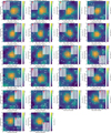 |
Fig. A.1 TESS target pixel file images of TOI-2095 for the 22 sectors analyzed in this work (made with tpfplotter, Aller et al. 2020). |
Appendix B Ground-based light curves
In this section we present the ground-based light curves for TOI-2095b and TOI-2095c taken with LCOGT and MuSCAT3 (see Figs. B.2 and B.1).
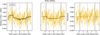 |
Fig. B.1 LCOGT ground-based transit observations of TOI-2095c. Left panel: Transit observations and best fitted model (black line). Middle panel: Transit model and model after removing systematics. Right panel: Residuals of the fit. The central time of the transit is marked by the purple dotted line and the predicted ingress and egress by the black dashed line. |
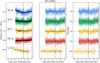 |
Fig. B.2 MuSCAT3 and LCOGT ground-based transit observations of TOI-2095b. Middle panel: Transit data and model after removing systematics. Right panel: Residuals of the fit. The central time of the transit is marked by the purple dotted line and the predicted ingress and egress by the black-dashed line. |
Appendix C Radial velocity data
In Tables C.1 and C.2, we present RV measurements taken with CARMENES visible channel and line activity indicators of TOI-2095 computed using SERVAL. Table C.3 presents the CCF activity indicators computed with raccoon. Figure C.1 shows the CARMENES RV measurements for the visible and near-infrared channels.
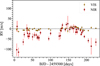 |
Fig. C.1 Radial velocity measurements obtained using SERVAL for the visible (VIS) and near-infrared (NIR) CARMENES arms. |
CARMENES visual channel radial velocity measurements of TOI-2095 computed by SERVAL.
CARMENES spectroscopic line activity indicators for TOI-2095 computed by SERVAL.
CARMENES activity indicators from cross-correlation for TOI-2095 computed by raccoon.
Appendix D TESS light curves and radial velocity joint fit
Figure D.1 shows the correlation between the Call activity index and the RV measurements taken with CARMENES. Figure D.3 shows the parameter distributions for the joint fit, where the GP parameters for the transit and RV fit were left out intentionally. Figure D.4 shows the photometry from the TESS sectors analyzed in this work and the best transit model including systematic effects. Tables D.1 and D.2 present the central transit times for TOI-2095b and TOI-2095c measured with PyTTV, respectively.
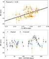 |
Fig. D.1 Radial velocity and Ca II stellar activity index correction. Top panel: RV measurements versus Ca IRTa activity index, the black line represents a linear fit to the data. Bottom panel: Uncorrected (orange circles) and activity-corrected (blue squares) RV measurements. |
Measured central time of transit and uncertainties for TESS data of TOI-2095b.
Measured central time of transit and uncertainties for TESS data of TOI-2095C.
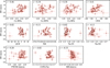 |
Fig. D.2 Radial velocity measurements versus activity indices. In each panel, the Pearson product-moment correlation coefficient r is shown. |
 |
Fig. D.3 Correlation plot for the fitted transit and orbital parameter. The free parameters used to model the systematic effects were intentionally left out for easy viewing. The blue lines marks the median values of the distribution. For plotting purposes the distributions for the central time of the transit and orbital period were offset by T1 = 2459240 days and P1 = 17 days for TOI-2095b and T2 = 2459239 days and P2 = 28 days for TOI-2095c, respectively. |
 |
Fig. D.4 TESS photometric observations of TOI-2095 and best fitting transit model including systematic effects (black line). The central transit time of TOI-2095b and TOI-2095c are marked by the orange and blue vertical lines, respectively. |
References
- Agol, E., Steffen, J., Sari, R., & Clarkson, W. 2005, MNRAS, 359, 567 [Google Scholar]
- Aller, A., Lillo-Box, J., Jones, D., Miranda, L. F., & Barceló Forteza, S. 2020, A&A, 635, A128 [NASA ADS] [CrossRef] [EDP Sciences] [Google Scholar]
- Ambikasaran, S., Foreman-Mackey, D., Greengard, L., Hogg, D. W., & ONeil, M. 2015, IEEE Trans. Pattern Anal. Mach. Intell., 38, 252 [Google Scholar]
- Bailer-Jones, C. A. L., Rybizki, J., Fouesneau, M., Demleitner, M., & Andrae, R. 2021, AJ, 161, 147 [Google Scholar]
- Batalha, N. E., Lewis, N. K., Line, M. R., Valenti, J., & Stevenson, K. 2018, ApJ, 856, L34 [NASA ADS] [CrossRef] [Google Scholar]
- Bauer, F. F., Zechmeister, M., & Reiners, A. 2015, A&A, 581, A117 [NASA ADS] [CrossRef] [EDP Sciences] [Google Scholar]
- Bauer, F. F., Zechmeister, M., Kaminski, A., et al. 2020, A&A, 640, A50 [NASA ADS] [CrossRef] [EDP Sciences] [Google Scholar]
- Benz, W., Broeg, C., Fortier, A., et al. 2021, Exp. Astron., 51, 109 [Google Scholar]
- Bonfils, X., Delfosse, X., Udry, S., et al. 2005, A&A, 442, 635 [NASA ADS] [CrossRef] [EDP Sciences] [Google Scholar]
- Borsato, L., Piotto, G., Gandolfi, D., et al. 2021, MNRAS, 506, 3810 [NASA ADS] [CrossRef] [Google Scholar]
- Brown, T. M., Baliber, N., Bianco, F. B., et al. 2013, PASP, 125, 1031 [Google Scholar]
- Caballero, J. A., Cortés-Contreras, M., Alonso-Floriano, F. J., et al. 2016a, in 19th Cambridge Workshop on Cool Stars, Stellar Systems, and the Sun (CS19), 148 [Google Scholar]
- Caballero, J. A., Guàrdia, J., López del Fresno, M., et al. 2016b, SPIE Conf. Ser., 9910, 99100E [Google Scholar]
- Cabrera, J., Barros, S. C. C., Armstrong, D., et al. 2017, A&A, 606, A75 [NASA ADS] [CrossRef] [EDP Sciences] [Google Scholar]
- Casagrande, L., Flynn, C., & Bessell, M. 2008, MNRAS, 389, 585 [Google Scholar]
- Casagrande, L., Schönrich, R., Asplund, M., et al. 2011, A&A, 530, A138 [NASA ADS] [CrossRef] [EDP Sciences] [Google Scholar]
- Castro González, A., Díez Alonso, E., Menéndez Blanco, J., et al. 2020, MNRAS, 499, 5416 [CrossRef] [Google Scholar]
- Castro-González, A., Díez Alonso, E., Menéndez Blanco, J., et al. 2022, MNRAS, 509, 1075 [Google Scholar]
- Castro-González, A., Demangeon, O. D. S., Lillo-Box, J., et al. 2023, A&A, 675, A52 [NASA ADS] [CrossRef] [EDP Sciences] [Google Scholar]
- Cepa, J., Aguiar, M., Escalera, V. G., et al. 2000, SPIE Conf. Ser., 4008, 623 [Google Scholar]
- Chen, J., & Kipping, D. 2017, ApJ, 834, 17 [Google Scholar]
- Christiansen, J. L., Bhure, S., Zink, J. K., et al. 2022, AJ, 163, 244 [NASA ADS] [CrossRef] [Google Scholar]
- Cifuentes, C., Caballero, J. A., Cortés-Contreras, M., et al. 2020, A&A, 642, A115 [NASA ADS] [CrossRef] [EDP Sciences] [Google Scholar]
- Cincotta, P. M., & Simó, C. 2000, A&AS, 147, 205 [NASA ADS] [CrossRef] [EDP Sciences] [Google Scholar]
- Cincotta, P. M., Giordano, C. M., & Simó, C. 2003, Physica D Nonlinear Phenomena, 182, 151 [NASA ADS] [CrossRef] [Google Scholar]
- Collins, K. A., Kielkopf, J. F., Stassun, K. G., & Hessman, F. V. 2017, AJ, 153, 77 [Google Scholar]
- Colome, J., & Ribas, I. 2006, IAU Special Session, 6, 11 [Google Scholar]
- Cortés Contreras, M. 2017, Ph.D. Thesis, Complutense University of Madrid, Spain [Google Scholar]
- Cumming, A., Marcy, G. W., & Butler, R. P. 1999, ApJ, 526, 890 [Google Scholar]
- Curtis, J. L., Agüeros, M. A., Matt, S. P., et al. 2020, ApJ, 904, 140 [Google Scholar]
- Cutri, R. M., Wright, E. L., Conrow, T., et al. 2021, VizieR Online Data Catalog: II/328 [Google Scholar]
- de Leon, J. P., Livingston, J., Endl, M., et al. 2021, MNRAS, 508, 195 [NASA ADS] [CrossRef] [Google Scholar]
- Delrez, L., Ehrenreich, D., Alibert, Y., et al. 2021, Nat. Astron., 5, 775 [NASA ADS] [CrossRef] [Google Scholar]
- Delrez, L., Murray, C. A., Pozuelos, F. J., et al. 2022, A&A, 667, A59 [NASA ADS] [CrossRef] [EDP Sciences] [Google Scholar]
- Demory, B. O., Pozuelos, F. J., Gómez Maqueo Chew, Y., et al. 2020, A&A, 642, A49 [NASA ADS] [CrossRef] [EDP Sciences] [Google Scholar]
- Dévora-Pajares, M., & Pozuelos, F. J. 2022, https://zenodo.org/record/6570832 [Google Scholar]
- Dhillon, V. S., Bezawada, N., Black, M., et al. 2021, MNRAS, 507, 350 [NASA ADS] [CrossRef] [Google Scholar]
- Dittmann, J. A., Irwin, J. M., Charbonneau, D., et al. 2017, Nature, 544, 333 [NASA ADS] [CrossRef] [Google Scholar]
- Dorn, C., & Lichtenberg, T. 2021, ApJ, 922, L4 [NASA ADS] [CrossRef] [Google Scholar]
- Dressing, C. D., & Charbonneau, D. 2015, ApJ, 807, 45 [Google Scholar]
- Fabrycky, D. C., Lissauer, J. J., Ragozzine, D., et al. 2014, ApJ, 790, 146 [Google Scholar]
- Faria, J. P., Suárez Mascareño, A., Figueira, P., et al. 2022, A&A, 658, A115 [NASA ADS] [CrossRef] [EDP Sciences] [Google Scholar]
- Feinstein, A. D., Schlieder, J. E., Livingston, J. H., et al. 2019, AJ, 157, 40 [NASA ADS] [CrossRef] [Google Scholar]
- Foreman-Mackey, D., Hogg, D. W., Lang, D., & Goodman, J. 2013, PASP, 125, 306 [Google Scholar]
- Frith, J., Pinfield, D. J., Jones, H. R. A., et al. 2013, MNRAS, 435, 2161 [Google Scholar]
- Fulton, B. J., Petigura, E. A., Howard, A. W., et al. 2017, AJ, 154, 109 [Google Scholar]
- Fulton, B. J., Petigura, E. A., Blunt, S., & Sinukoff, E. 2018, PASP, 130, 044504 [Google Scholar]
- Furlan, E., Ciardi, D. R., Everett, M. E., et al. 2017, AJ, 153, 71 [NASA ADS] [CrossRef] [Google Scholar]
- Gagné, J., Mamajek, E. E., Malo, L., et al. 2018, ApJ, 856, 23 [Google Scholar]
- Gaia Collaboration (Vallenari, A., et al.) 2023, A&A, 674, A1 [NASA ADS] [CrossRef] [EDP Sciences] [Google Scholar]
- Gardner, J. P., Mather, J. C., Clampin, M., et al. 2006, Space Sci. Rev., 123, 485 [Google Scholar]
- Giacalone, S., Dressing, C. D., Jensen, E. L. N., et al. 2021, AJ, 161, 24 [Google Scholar]
- Gillon, M., Jehin, E., Lederer, S. M., et al. 2016, Nature, 533, 221 [Google Scholar]
- Gillon, M., Triaud, A. H. M. J., Demory, B.-O., et al. 2017, Nature, 542, 456 [NASA ADS] [CrossRef] [Google Scholar]
- Guerrero, N. M., Seager, S., Huang, C. X., et al. 2021, ApJS, 254, 39 [NASA ADS] [CrossRef] [Google Scholar]
- Günther, M. N., & Daylan, T. 2021, ApJS, 254, 13 [CrossRef] [Google Scholar]
- Günther, M. N., Zhan, Z., Seager, S., et al. 2020, AJ, 159, 60 [Google Scholar]
- Hadden, S. 2019, https://zenodo.org/record/3356829 [Google Scholar]
- He, M. Y., Ford, E. B., Ragozzine, D., & Carrera, D. 2020, AJ, 160, 276 [Google Scholar]
- Hilton, E. J., West, A. A., Hawley, S. L., & Kowalski, A. F. 2010, AJ, 140, 1402 [Google Scholar]
- Hippke, M., & Heller, R. 2019, A&A, 623, A39 [NASA ADS] [CrossRef] [EDP Sciences] [Google Scholar]
- Hippke, M., David, T. J., Mulders, G. D., & Heller, R. 2019, AJ, 158, 143 [Google Scholar]
- Hobson, M. J., Jofré, E., García, L., Petrucci, R., & Gómez, M. 2018, Rev. Mex. Astron. Astrofis., 54, 65 [NASA ADS] [Google Scholar]
- Holman, M. J., & Murray, N. W. 2005, Science, 307, 1288 [Google Scholar]
- Ingersoll, A. P. 1969, J. Atmos. Sci., 26, 1191 [NASA ADS] [CrossRef] [Google Scholar]
- Jeffers, S. V., Schöfer, P., Lamert, A., et al. 2018, A&A, 614, A76 [NASA ADS] [CrossRef] [EDP Sciences] [Google Scholar]
- Jenkins, J. M. 2002, ApJ, 575, 493 [Google Scholar]
- Jenkins, J. M., Twicken, J. D., McCauliff, S., et al. 2016, SPIE Conf. Ser., 9913, 99133E [Google Scholar]
- Jenkins, J. S., Pozuelos, F. J., Tuomi, M., et al. 2019, MNRAS, 490, 5585 [Google Scholar]
- Jenkins, J. M., Tenenbaum, P., Seader, S., et al. 2020, Kepler Data Processing Handbook: Transiting Planet Search, Kepler Science Document KSCI-19081-003 [Google Scholar]
- Jensen, E. 2013, Astrophysics Source Code Library [record ascl:1306.007] [Google Scholar]
- Kaltenegger, L., Pepper, J., Stassun, K., & Oelkers, R. 2019, ApJ, 874, L8 [NASA ADS] [CrossRef] [Google Scholar]
- Kanodia, S., Wolfgang, A., Stefánsson, G. K., Ning, B., & Mahadevan, S. 2019, ApJ, 882, 38 [NASA ADS] [CrossRef] [Google Scholar]
- Kasting, J. F. 1988, Icarus, 74, 472 [NASA ADS] [CrossRef] [Google Scholar]
- Kipping, D. M. 2013, MNRAS, 435, 2152 [Google Scholar]
- Kopparapu, R. K., Ramirez, R., Kasting, J. F., et al. 2013, ApJ, 765, 131 [NASA ADS] [CrossRef] [Google Scholar]
- Kossakowski, D., Kürster, M., Trifonov, T., et al. 2023, A&A, 670, A84 [NASA ADS] [CrossRef] [EDP Sciences] [Google Scholar]
- Lafarga, M., Ribas, I., Lovis, C., et al. 2020, A&A, 636, A36 [NASA ADS] [CrossRef] [EDP Sciences] [Google Scholar]
- Lam, K. W. F., Csizmadia, S., Astudillo-Defru, N., et al. 2021, Science, 374, 1271 [NASA ADS] [CrossRef] [Google Scholar]
- Latham, D. W., Rowe, J. F., Quinn, S. N., et al. 2011, ApJ, 732, L24 [NASA ADS] [CrossRef] [Google Scholar]
- Lépine, S., & Gaidos, E. 2011, AJ, 142, 138 [Google Scholar]
- Lépine, S., & Shara, M. M. 2005, AJ, 129, 1483 [Google Scholar]
- Li, J., Tenenbaum, P., Twicken, J. D., et al. 2019, PASP, 131, 024506 [NASA ADS] [CrossRef] [Google Scholar]
- Lillo-Box, J., Figueira, P., Leleu, A., et al. 2020, A&A, 642, A121 [NASA ADS] [CrossRef] [EDP Sciences] [Google Scholar]
- Lillo-Box, J., Santos, N. C., Santerne, A., et al. 2022, A&A, 667, A102 [NASA ADS] [CrossRef] [EDP Sciences] [Google Scholar]
- Limbach, M. A., & Turner, E. L. 2015, PNAS, 112, 20 [NASA ADS] [CrossRef] [Google Scholar]
- Lissauer, J. J., Ragozzine, D., Fabrycky, D. C., et al. 2011, ApJS, 197, 8 [Google Scholar]
- Lissauer, J. J., Marcy, G. W., Rowe, J. F., et al. 2012, ApJ, 750, 112 [NASA ADS] [CrossRef] [Google Scholar]
- Livingston, J. H., Crossfield, I. J. M., Petigura, E. A., et al. 2018, AJ, 156, 277 [NASA ADS] [CrossRef] [Google Scholar]
- Lopez, E. D., & Rice, K. 2018, MNRAS, 479, 5303 [NASA ADS] [CrossRef] [Google Scholar]
- Luque, R., & Pallé, E. 2022, Science, 377, 1211 [NASA ADS] [CrossRef] [Google Scholar]
- Luque, R., Nowak, G., Pallé, E., et al. 2018, A&A, 620, A171 [NASA ADS] [CrossRef] [EDP Sciences] [Google Scholar]
- Marfil, E., Tabernero, H. M., Montes, D., et al. 2021, A&A, 656, A162 [NASA ADS] [CrossRef] [EDP Sciences] [Google Scholar]
- Martinez, C. F., Cunha, K., Ghezzi, L., & Smith, V. V. 2019, ApJ, 875, 29 [Google Scholar]
- Martínez-Rodríguez, H., Caballero, J. A., Cifuentes, C., Piro, A. L., & Barnes, R. 2019, ApJ, 887, 261 [Google Scholar]
- Masci, F. J., Laher, R. R., Rusholme, B., et al. 2019, PASP, 131, 018003 [Google Scholar]
- Mayo, A. W., Vanderburg, A., Latham, D. W., et al. 2018, AJ, 155, 136 [Google Scholar]
- McCully, C., Volgenau, N. H., Harbeck, D.-R., et al. 2018, SPIE Conf. Ser., 10707, 107070K [Google Scholar]
- Montes, D., López-Santiago, J., Gálvez, M. C., et al. 2001, MNRAS, 328, 45 [NASA ADS] [CrossRef] [Google Scholar]
- Montet, B. T., Morton, T. D., Foreman-Mackey, D., et al. 2015, ApJ, 809, 25 [Google Scholar]
- Mordasini, C. 2020, A&A, 638, A52 [NASA ADS] [CrossRef] [EDP Sciences] [Google Scholar]
- Morris, R. L., Twicken, J. D., Smith, J. C., et al. 2020, Kepler Data Processing Handbook: Photometric Analysis, Kepler Science Document KSCI-19081-003 [Google Scholar]
- Morton, T. D. 2012, ApJ, 761, 6 [NASA ADS] [CrossRef] [Google Scholar]
- Morton, T. D. 2015, Astrophysics Source Code Library [record ascl:1503.011] [Google Scholar]
- Mousis, O., Deleuil, M., Aguichine, A., et al. 2020, ApJ, 896, L22 [NASA ADS] [CrossRef] [Google Scholar]
- Mugrauer, M., & Michel, K.-U. 2020, Astron. Nachr., 341, 996 [NASA ADS] [CrossRef] [Google Scholar]
- Mugrauer, M., & Michel, K.-U. 2021, Astron. Nachr., 342, 840 [NASA ADS] [CrossRef] [Google Scholar]
- Murgas, F., Astudillo-Defru, N., Bonfils, X., et al. 2021, A&A, 653, A60 [NASA ADS] [CrossRef] [EDP Sciences] [Google Scholar]
- Narita, N., Fukui, A., Yamamuro, T., et al. 2020, SPIE Conf. Ser., 11447, 114475K [NASA ADS] [Google Scholar]
- Ning, B., Wolfgang, A., & Ghosh, S. 2018, ApJ, 869, 5 [NASA ADS] [CrossRef] [Google Scholar]
- Owen, J. E., & Wu, Y. 2013, ApJ, 775, 105 [Google Scholar]
- Parviainen, H. 2015, MNRAS, 450, 3233 [Google Scholar]
- Parviainen, H., & Aigrain, S. 2015, MNRAS, 453, 3821 [Google Scholar]
- Passegger, V. M., Reiners, A., Jeffers, S. V., et al. 2018, A&A, 615, A6 [NASA ADS] [CrossRef] [EDP Sciences] [Google Scholar]
- Perryman, M. 2011, The Exoplanet Handbook (Cambridge University Press) [Google Scholar]
- Pozuelos, F. J., Suárez, J. C., de Elía, G. C., et al. 2020, A&A, 641, A23 [NASA ADS] [CrossRef] [EDP Sciences] [Google Scholar]
- Pozuelos, F. J., Timmermans, M., Rackham, B. V., et al. 2023, A&A, 672, A70 [NASA ADS] [CrossRef] [EDP Sciences] [Google Scholar]
- Quintana, E. V., Barclay, T., Raymond, S. N., et al. 2014, Science, 344, 277 [NASA ADS] [CrossRef] [Google Scholar]
- Quirrenbach, A., Amado, P. J., Caballero, J. A., et al. 2014, Proc. SPIE, 9147, 91471F [Google Scholar]
- Quirrenbach, A., Amado, P. J., Ribas, I., et al. 2018, SPIE Conf. Ser., 10702, 107020W [Google Scholar]
- Rein, H., & Liu, S. F. 2012, A&A, 537, A128 [NASA ADS] [CrossRef] [EDP Sciences] [Google Scholar]
- Rein, H., & Tamayo, D. 2015, MNRAS, 452, 376 [Google Scholar]
- Reiners, A., Zechmeister, M., Caballero, J. A., et al. 2018, A&A, 612, A49 [NASA ADS] [CrossRef] [EDP Sciences] [Google Scholar]
- Ricker, G. R., Winn, J. N., Vanderspek, R., et al. 2014, SPIE Conf. Ser., 9143, 914320 [Google Scholar]
- Rodriguez, J. E., Vanderburg, A., Zieba, S., et al. 2020, AJ, 160, 117 [NASA ADS] [CrossRef] [Google Scholar]
- Rojas-Ayala, B., Covey, K. R., Muirhead, P. S., & Lloyd, J. P. 2010, ApJ, 720, L113 [Google Scholar]
- Rowe, J. F., Bryson, S. T., Marcy, G. W., et al. 2014, ApJ, 784, 45 [Google Scholar]
- Safonov, B. S., Lysenko, P. A., & Dodin, A. V. 2017, Astron. Lett., 43, 344 [NASA ADS] [CrossRef] [Google Scholar]
- Schanche, N., Pozuelos, F. J., Günther, M. N., et al. 2022, A&A, 657, A45 [NASA ADS] [CrossRef] [EDP Sciences] [Google Scholar]
- Schweitzer, A., Passegger, V. M., Cifuentes, C., et al. 2019, A&A, 625, A68 [NASA ADS] [CrossRef] [EDP Sciences] [Google Scholar]
- Shields, A. L., Ballard, S., & Johnson, J. A. 2016, Phys. Rep., 663, 1 [NASA ADS] [CrossRef] [Google Scholar]
- Skrutskie, M. F., Cutri, R. M., Stiening, R., et al. 2006, AJ, 131, 1163 [NASA ADS] [CrossRef] [Google Scholar]
- Smith, J. C., Stumpe, M. C., Van Cleve, J. E., et al. 2012, PASP, 124, 1000 [Google Scholar]
- Southworth, J. 2011, MNRAS, 417, 2166 [Google Scholar]
- Stassun, K. G., Oelkers, R. J., Pepper, J., et al. 2018, AJ, 156, 102 [Google Scholar]
- Stefánsson, G., Kopparapu, R., Lin, A., et al. 2020, AJ, 160, 259 [CrossRef] [Google Scholar]
- Stelzer, B., Bogner, M., Magaudda, E., & Raetz, S. 2022, A&A, 665, A30 [NASA ADS] [CrossRef] [EDP Sciences] [Google Scholar]
- Stumpe, M. C., Smith, J. C., Van Cleve, J. E., et al. 2012, PASP, 124, 985 [Google Scholar]
- Stumpe, M. C., Smith, J. C., Catanzarite, J. H., et al. 2014, PASP, 126, 100 [Google Scholar]
- Suárez Mascareño, A., Faria, J. P., Figueira, P., et al. 2020, A&A, 639, A77 [Google Scholar]
- Suárez Mascareno, A., Damasso, M., Lodieu, N., et al. 2021, Nat. Astron., 6, 232 [Google Scholar]
- Suissa, G., Mandell, A. M., Wolf, E. T., et al. 2020, ApJ, 891, 58 [NASA ADS] [CrossRef] [Google Scholar]
- Tabernero, H. M., Marfil, E., Montes, D., & González Hernández, J. I. 2022, A&A, 657, A66 [NASA ADS] [CrossRef] [EDP Sciences] [Google Scholar]
- Tamayo, D., Cranmer, M., Hadden, S., et al. 2020, PNAS, 117, 18194 [CrossRef] [PubMed] [Google Scholar]
- Terrien, R. C., Mahadevan, S., Bender, C. F., et al. 2012, ApJ, 747, L38 [NASA ADS] [CrossRef] [Google Scholar]
- Torres, G., Kane, S. R., Rowe, J. F., et al. 2017, AJ, 154, 264 [NASA ADS] [CrossRef] [Google Scholar]
- Trifonov, T., Kürster, M., Zechmeister, M., et al. 2018, A&A, 609, A117 [NASA ADS] [CrossRef] [EDP Sciences] [Google Scholar]
- Turbet, M., Ehrenreich, D., Lovis, C., Bolmont, E., & Fauchez, T. 2019, A&A, 628, A12 [NASA ADS] [CrossRef] [EDP Sciences] [Google Scholar]
- Turbet, M., Bolmont, E., Ehrenreich, D., et al. 2020, A&A, 638, A41 [NASA ADS] [CrossRef] [EDP Sciences] [Google Scholar]
- Twicken, J. D., Catanzarite, J. H., Clarke, B. D., et al. 2018, PASP, 130, 064502 [Google Scholar]
- Virtanen, P., Gommers, R., Oliphant, T. E., et al. 2020, Nat. Methods, 17, 261 [Google Scholar]
- Wells, R. D., Rackham, B. V., Schanche, N., et al. 2021, A&A, 653, A97 [NASA ADS] [CrossRef] [EDP Sciences] [Google Scholar]
- Wisdom, J., & Holman, M. 1991, AJ, 102, 1528 [Google Scholar]
- Wizinowich, P., Acton, D. S., Shelton, C., et al. 2000, PASP, 112, 315 [NASA ADS] [CrossRef] [Google Scholar]
- Wu, Y. 2019, ApJ, 874, 91 [NASA ADS] [CrossRef] [Google Scholar]
- Zacharias, N., Finch, C. T., Girard, T. M., et al. 2013, AJ, 145, 44 [Google Scholar]
- Zechmeister, M., & Kürster, M. 2009, A&A, 496, 577 [CrossRef] [EDP Sciences] [Google Scholar]
- Zechmeister, M., Anglada-Escudé, G., & Reiners, A. 2014, A&A, 561, A59 [NASA ADS] [CrossRef] [EDP Sciences] [Google Scholar]
- Zechmeister, M., Reiners, A., Amado, P. J., et al. 2018, A&A, 609, A12 [NASA ADS] [CrossRef] [EDP Sciences] [Google Scholar]
- Zeng, L., Sasselov, D. D., & Jacobsen, S. B. 2016, ApJ, 819, 127 [Google Scholar]
- Zeng, L., Jacobsen, S. B., Sasselov, D. D., et al. 2019, PNAS, 116, 9723 [Google Scholar]
- Zhu, W., Petrovich, C., Wu, Y., Dong, S., & Xie, J. 2018, ApJ, 860, 101 [Google Scholar]
- Ziegler, C., Tokovinin, A., Briceflo, C., et al. 2020, AJ, 159, 19 [Google Scholar]
- Zinzi, A., & Turrini, D. 2017, A&A, 605, L4 [NASA ADS] [CrossRef] [EDP Sciences] [Google Scholar]
- Zsom, A., Seager, S., de Wit, J., & Stamenković, V. 2013, ApJ, 778, 109 [NASA ADS] [CrossRef] [Google Scholar]
NASA Exoplanet Archive: https://exoplanetarchive.ipac.caltech.edu/
From TESS follow-up recon spectroscopy group (SG2), based on predicted masses values computed using Chen & Kipping (2017).
SHERLOCK (Searching for Hints of Exoplanets fRom Lightcurves Of spaCe-based seeKers) code is fully available on GitHub: https://github.com/franpoz/SHERLOCK
The MATRIX (Multi-phAse Transits Recovery from Injected eXoplanets) code is open access on GitHub: https://github.com/PlanetHunters/tkmatrix
All Tables
Posterior probabilities for the EB, BEB, HEB, and planet scenarios for TOI-2095b and TOI-2095c as computed with vespa.
CARMENES visual channel radial velocity measurements of TOI-2095 computed by SERVAL.
CARMENES spectroscopic line activity indicators for TOI-2095 computed by SERVAL.
CARMENES activity indicators from cross-correlation for TOI-2095 computed by raccoon.
All Figures
|
Fig. 1 High-resolution imaging of TOI-2095. Left panel: Keck NIR AO imaging and sensitivity curve for TOI-2095 taken in the Br-γ filter. The image reaches a contrast of ~7.4 magnitudes fainter than the host star within 0.″5. Inset: image of the central portion of the data. Right panel: speckle sensitivity curve of TOI-2095 taken with the SPeckle Polarimeter (SPP) at the Caucasian Observatory of Sternberg Astronomical Institute (SAI). Inset: speckle autocorrelation function. |
| In the text | |
|
Fig. 2 Long-term photometric follow-up of TOI-2095 from ZTF (z band) and TJO (R band). Left panels: photometric time-series and joint best fitted model computed using GP adopting a quasi-periodic kernel (black line). The 1σ uncertainty regions of the fit are shown in light blue. The residuals of the fit are shown at the bottom panels. Right panels: GLS periodogram (Zechmeister & Kürster 2009) for each photometric data set. The vertical green line shows the fitted rotational period of the star. The horizontal lines represent the FAP levels of 10% (red dotted line) and 1% (blue dashed line). |
| In the text | |
|
Fig. 3 GLS periodograms of the CARMENES RV measurements taken with the optical channel, spectral activity indices, and window function. The horizontal lines represent the false alarm probability (FAP) levels of 10% (red dotted line) and 1% (green dash line). The vertical lines mark the period of planets TOI-2095b (P = 17.66 days, solid orange line), TOI-2095c (P = 28.17 days, solid blue line), and the measured rotation period of the star from photometric observations (P = 40 days: dashed brown line). |
| In the text | |
|
Fig. 4 TESS phase-folded light curves after subtracting the photometric variability for TOI-2095b (top left) and TOI-2095c (top right). The best-fit model is shown in black, the circles are TESS binned data points, and the points are individual TESS observations. Bottom panels: residuals of the fit. |
| In the text | |
|
Fig. 5 Radial velocity measurements of TOI-2095 taken with CARMENES. (a): RV time series and best-fitting model (blue line) including red noise. The plotted RV model was computed using the median values of the posterior distribution for each fitted parameter. The shaded area around the blue line represent the 1σ uncertainty levels of the fitted model. (b): residuals of the fit after subtracting the two planet models. (c) and (d): phase-folded RV measurements after subtracting the red noise and best-fit model (blue line). |
| In the text | |
|
Fig. 6 Posterior distributions for the planetary masses of TOI-2095b and TOI-2095c. The vertical dashed blue line represents the 95% confidence limit for each planet; for TOI-2095b, we And a mass upper limit of Mb < 4.1 Μ⊕ and for TOI-2095c, it is Mc < 7.4 M⊕. |
| In the text | |
|
Fig. 7 Central mid-transit times measured using TESS data for TOI-2095b (top panel) and TOI-2095c (bottom panel). The shaded areas represent the 1σ and 3σ uncertainty limits for the central time of the transit measurements. |
| In the text | |
|
Fig. 8 Injection-and-recovery experiment performed to test the detectability of inner planets in the system using the TESS sectors described in Sect. 2. We explored a total of 3000 different scenarios. Each pixel evaluated about eight scenarios, that is, eight light curves with injected planets having different Pplanet, Rplanet, and T0. Higher recovery rates are presented in yellow and green colors, while lower recovery rates are shown in blue and darker hues. Planets smaller than 1.0 R⊕ would remain undetected for the explored periods. |
| In the text | |
|
Fig. 9 Stability map of the TOI-2095 system in the eb – ec parameter space based on the MEGNO chaos indicator. The map consists of a 20 × 20 grid, where each grid cell is the average of 10 realizations with randomized mean anomalies and arguments of periastron. The three regions of differing stability (A, B, C) are marked with letters and are described by Eqs. (5) and (6). |
| In the text | |
|
Fig. 10 Stability map of TOI-2095 for a hypothetical third planet in the system. Top panel: stability map for a third planet in a circular orbit case. Each cell of the 200 × 200 grid considers a different combination of ad and Md and represents the average value of 10 randomized realizations of the system’s initial conditions (i, ω, M). Bottom panel: stability map for a third planet in a eccentric orbit case. The map consists of 100 x 100 grid cells plotted in the ad – ed space. In both panels, the colorbar indicates the probability of stability from SPOCK (Tamayo et al. 2020). The vertical dashed lines denote the locations of TOI-2095b (cyan) and TOI-2095c (green). |
| In the text | |
|
Fig. 11 Expected TTVs amplitudes for planets TOI-2095b (upper panel) and TOI-2095c (lower panel). Dashed and solid vertical lines correspond to the mode and the mean of the PDF, respectively. |
| In the text | |
|
Fig. 12 Mass-radius diagramofall known transiting exoplanets taken from TepCat(Southworth 2011). Theupperlimits forthe masses of TOI-2095b and TOI-2095c derived from RV measurements (Mb < 4.1 M⊕ and Mc < 7.4 M⊕ respectively) are delimited by the black arrows. The predicted masses and uncertainties for TOI-2095b and TOI-2095c computed with the mass-radius relations of Chen & Kipping (2017, left) and Kanodia et al. (2019, right) are marked by the yellow and light blue star respectively. We show planets with P < 30 days and with mass determinations with an uncertainty better than 30%. Planets around stars with Teff ≤ 4000 K and Teff > 4000 K are marked by orange circles and blue triangles, respectively. The lines represent the composition models of Zeng et al. (2016, 2019) for pure iron cores (100% Fe, brown solid line), Earth-like rocky compositions (32.5% Fe plus 67.5% MgSiO3, dash green line), and a water world (0.1% H2 envelope plus 49.95% Earth-like rocky core plus 49.95% H2O, dash-dotted blue line). |
| In the text | |
|
Fig. 13 Incident flux in Earth units versus stellar effective temperature for known exoplanets (data taken from NASA Exoplanet Archive). The color of each circle represents the equilibrium temperature of the planet. The habitable zone limits of Kopparapu et al. (2013) are shown with lines. The position of TOI-2095b and TOI-2095c are marked by the green stars. |
| In the text | |
|
Fig. A.1 TESS target pixel file images of TOI-2095 for the 22 sectors analyzed in this work (made with tpfplotter, Aller et al. 2020). |
| In the text | |
|
Fig. B.1 LCOGT ground-based transit observations of TOI-2095c. Left panel: Transit observations and best fitted model (black line). Middle panel: Transit model and model after removing systematics. Right panel: Residuals of the fit. The central time of the transit is marked by the purple dotted line and the predicted ingress and egress by the black dashed line. |
| In the text | |
|
Fig. B.2 MuSCAT3 and LCOGT ground-based transit observations of TOI-2095b. Middle panel: Transit data and model after removing systematics. Right panel: Residuals of the fit. The central time of the transit is marked by the purple dotted line and the predicted ingress and egress by the black-dashed line. |
| In the text | |
|
Fig. C.1 Radial velocity measurements obtained using SERVAL for the visible (VIS) and near-infrared (NIR) CARMENES arms. |
| In the text | |
|
Fig. D.1 Radial velocity and Ca II stellar activity index correction. Top panel: RV measurements versus Ca IRTa activity index, the black line represents a linear fit to the data. Bottom panel: Uncorrected (orange circles) and activity-corrected (blue squares) RV measurements. |
| In the text | |
|
Fig. D.2 Radial velocity measurements versus activity indices. In each panel, the Pearson product-moment correlation coefficient r is shown. |
| In the text | |
|
Fig. D.3 Correlation plot for the fitted transit and orbital parameter. The free parameters used to model the systematic effects were intentionally left out for easy viewing. The blue lines marks the median values of the distribution. For plotting purposes the distributions for the central time of the transit and orbital period were offset by T1 = 2459240 days and P1 = 17 days for TOI-2095b and T2 = 2459239 days and P2 = 28 days for TOI-2095c, respectively. |
| In the text | |
|
Fig. D.4 TESS photometric observations of TOI-2095 and best fitting transit model including systematic effects (black line). The central transit time of TOI-2095b and TOI-2095c are marked by the orange and blue vertical lines, respectively. |
| In the text | |
Current usage metrics show cumulative count of Article Views (full-text article views including HTML views, PDF and ePub downloads, according to the available data) and Abstracts Views on Vision4Press platform.
Data correspond to usage on the plateform after 2015. The current usage metrics is available 48-96 hours after online publication and is updated daily on week days.
Initial download of the metrics may take a while.