| Issue |
A&A
Volume 677, September 2023
|
|
|---|---|---|
| Article Number | A173 | |
| Number of page(s) | 24 | |
| Section | Astrophysical processes | |
| DOI | https://doi.org/10.1051/0004-6361/202244608 | |
| Published online | 22 September 2023 | |
The persistence of magneto-rotational turbulence in gravitationally turbulent accretion disks
Physics Department of Bayreuth, Universitätsstraße 30, Bayreuth, Germany
e-mail: This email address is being protected from spambots. You need JavaScript enabled to view it.
Received:
27
July
2022
Accepted:
24
July
2023
Abstract
Aims. Our main goal is to probe the persistence of turbulence originating from the magneto-rotational instability (MRI) in gravito-turbulent disks. This state is referred to here as GI-MRI coexistence, with GI standing for gravitational instability. We test the influence of GI strength, controlled by the cooling law, and the impact of Ohmic resistivity.
Methods. Our starting point was three-dimensional, ideal, magnetohydrodynamic (MHD) simulations of gravitational turbulence in the local shearing-box approximation using the code Athena. We introduced a zero-net-flux magnetic seed field in a GI-turbulent state and investigated the nonlinear evolution. The GI strength was varied by modifying the cooling parameters. We tested the cooling times τcΩ0 = 10, τcΩ0 = 20, and τcΩ0 = 10, with additional background heating. For some resistive cases, ideal-MHD simulations, which had already developed GI-MRI coexistence, were restarted with a finite Ohmic resistivity enabled at the moment of restart.
Results. It appears that there are two possible saturated dynamo states in the ideal-MHD regime: a state of GI-MRI coexistence (for low GI activity) and a strong-GI dynamo. The cases with lower GI activity eventually develop a clearly visible butterfly pattern. For the case with the highest GI activity (τcΩ0 = 10, no heating), a clearly visible butterfly pattern is absent, though more chaotic field reversals are observed above (and below) the mid-plane. We were also able to reproduce the results of previous simulations. With Ohmic resistivity, the simulation outcome can be substantially different. There exists a critical magnetic Reynolds number, ⟨Rm⟩ ∼ 500, below which the ideal-MHD outcome is replaced by a new dynamo state. For larger Reynolds numbers, one recovers turbulent states that are more reminiscent of the ideal-MHD states, and especially the strong-GI case. This new state leads to oscillations, which are caused by a significant heat production due to the resistive dissipation of magnetic energy. The additional heat periodically quenches GI, and the quenching events correspond to maxima of the Toomre value, Q.
Key words: accretion / accretion disks / magnetic fields / instabilities / turbulence / dynamo
© The Authors 2023
 Open Access article, published by EDP Sciences, under the terms of the Creative Commons Attribution License (https://creativecommons.org/licenses/by/4.0), which permits unrestricted use, distribution, and reproduction in any medium, provided the original work is properly cited.
This article is published in open access under the Subscribe to Open model. This email address is being protected from spambots. You need JavaScript enabled to view it. to support open access publication.
1. Introduction
In accretion disks, instabilities are an important ingredient as they allow turbulence to emerge, which in turn leads to an effective viscosity that largely exceeds the molecular viscosity. The turbulent viscosity allows angular momentum to be transported outwards (Lynden-Bell 1969; Shakura & Sunyaev 1973; Balbus & Hawley 1998) and thereby allows the process of accretion to occur in the first place. Additionally, certain types of turbulence may also amplify existing magnetic fields by providing a dynamo mechanism (Brandenburg et al. 1995; Brandenburg & Donner 1997; Balbus & Hawley 1998; Rüdiger & Pipin 2000; Ziegler & Rüdiger 2000; Lesur & Ogilvie 2008; Gressel 2010; Salvesen et al. 2016).
Well-known examples of instabilities that sustain turbulence are the gravitational instability (GI; see e.g. Toomre 1964; Lin & Shu 1964; Gammie 2001; Kratter & Lodato 2016) and the magneto-rotational instability (MRI; Balbus & Hawley 1991, 1998; Hawley et al. 1995; Brandenburg et al. 1995). Many numerical studies have been dedicated to both GI (Gammie 2001; Lodato & Rice 2004; Cossins et al. 2009; Rice et al. 2011, 2003; Paardekooper 2012; Young & Clarke 2015; Boley et al. 2006; Shi & Chiang 2014; Riols et al. 2017; Riols & Latter 2018b; Booth & Clarke 2019; Hirose & Shi 2019; Zier & Springel 2023) and MRI (Hawley et al. 1995; Brandenburg et al. 1995; Stone et al. 1996; Suzuki & Inutsuka 2009; Guan & Gammie 2011; Shi et al. 2009; Simon et al. 2011; Käpylä & Korpi 2011; Bai & Stone 2013; Fromang et al. 2013; Coleman et al. 2017). This also includes interactions of the two instabilities. Interactions can occur indirectly via limit cycles, whereby different accretion rates associated with GI and MRI can lead to outbursts of accretion (see e.g. Armitage et al. 2001; Zhu et al. 2009, 2010; Martin & Lubow 2011; Martin et al. 2012). Whether MRI and GI directly coexist is less clear. Some local simulations seem to suggest that MRI is absent (see e.g. Riols & Latter 2018a, 2019), though there are global and local simulations that are consistent with GI-MRI coexistence (Fromang et al. 2004; Fromang 2005; Löhnert & Peeters 2022). It is generally found that GI can lead to dynamo activity (Riols & Latter 2018a, 2019; Riols et al. 2021; Deng et al. 2020; Löhnert & Peeters 2022; Béthune & Latter 2022). The interaction of the two instabilities may be important for disk systems that are both heavy enough to be gravitationally unstable,
 (1)
(1)
with Qc ≳ 1, and sufficiently ionised to trigger MRI, such as certain regions of active galactic nuclei (see e.g. Menou & Quataert 2001; Goodman 2003). It is noted that linear, axisymmetric GI occurs for Q < 1, though non-axisymmetric modes, or systems with additional cooling (heating) physics, can also become unstable for Q ≳ 1 (see e.g. Kratter & Lodato 2016; Lin & Kratter 2016). Riols & Latter (2019) studied the effect of Ohmic resistivity on the GI dynamo in more detail and conclude that the dynamo operates for a wide range of magnetic Reynolds numbers, Rm. The dynamo strength, indicated by the growth rate, is found to vary with the exact value of Rm. Magneto-rotational instability is assumed to be absent there. A similar behaviour was found for ambipolar diffusion by Riols et al. (2021).
In Löhnert & Peeters (2022), we reported that the ideal magnetohydrodynamic (MHD) case leads to a state that is consistent with GI-MRI coexistence. Some of the results shown in Löhnert & Peeters (2022) differ from similar, previous simulations (Riols & Latter 2018a, 2019). Hence, one goal of the present study is to identify possible reasons for theses differences and to further test the persistence of GI-MRI coexistence, by varying the GI strength (e.g. measured by α). This is achieved by modifying the cooling time and by including, or turning off, additional heating. Additionally, the influence of Ohmic resistivity on the dynamo state is tested.
We note that the MRI alone can lead to a more varied behaviour in the presence of resistivity (see e.g. Sano et al. 1998; Ziegler & Rüdiger 2001; Sano & Stone 2002; Fromang et al. 2007; Turner et al. 2007; Simon & Hawley 2009; Oishi & Mac Low 2011; Davis et al. 2010; Simon et al. 2011). This ranges from intermittent bursts of turbulent activity (Simon et al. 2011) to complete quenching, for example in dead zones of protoplanetary disks (see e.g. Turner et al. 2007; Armitage 2011). Magnetohydrodynamic simulations of GI with Ohmic resistivity were also investigated in Riols & Latter (2019), and cases with ambipolar diffusion were presented in Riols et al. (2021). The magnetic Reynolds numbers tested in Riols & Latter (2019) were in the range Rm ≲ 500. The dynamo states observed there differ from the states of GI-MRI coexistence found in Löhnert & Peeters (2022), though Riols & Latter (2019) also point out that the GI dynamo appears to change its state for Rm ≳ 500. We suspect that the new dynamo state might correspond to GI-MRI coexistence. Hence, the goal here is to probe this higher-Rm regime.
The structure of the paper is as follows: Sect. 2 provides a summary of the shearing-box model, including the equations of motion, and the additional physics that is used. Important definitions, quantities, and frequently used averages are detailed in Sect. 3. The applied numerical methods and Athena settings are outlined in Sect. 4. In Sect. 5 ideal-MHD simulations, with varying GI strength, are discussed. Two different saturation states of the dynamo are found, and the possibility of MRI presence in the weak-GI cases is elaborated on. The first resistive simulation (⟨Rm⟩∼280) is provided in Sect. 6, and important observations and differences from the ideal cases are highlighted. We find that the newly formed turbulent state (here referred to as ‘resistive-GI dynamo’) differs significantly from the ideal state of GI-MRI coexistence. We then show in Sect. 7.1 that the resistive-GI dynamo is obtained for ⟨Rm⟩≲500. Larger Rm values result in dynamo states that share similarities with the ideal-MHD regime, suggesting a state transition at ⟨Rm⟩∼500. In Sect. 7.2 we test whether the transition is indeed physical, and not an artefact of unresolved resistivity. Finally, in Sect. 8, we finish with a conclusion.
2. Model equations
The simulations presented here rely on the same model, as outlined in Löhnert & Peeters (2022). The model includes the equations of motion for MHD as well as self-gravity:
 (2a)
(2a)
 (2b)
(2b)
 (2c)
(2c)
![Mathematical equation: $$ \begin{aligned}&\partial _{\rm t} E + \nabla \cdot \left( \left[E + P + \frac{{\boldsymbol{B}}^2}{2\mu _0}\right]\boldsymbol{v} - \boldsymbol{B}(\boldsymbol{B}\cdot \boldsymbol{v}) \right) \nonumber \\&= -\rho \boldsymbol{v}\cdot \nabla \Phi + 3\Omega _0^2x\,{ v}_x - \Omega _0^2z\,{ v}_z + \rho \dot{q} \end{aligned} $$](/articles/aa/full_html/2023/09/aa44608-22/aa44608-22-eq5.gif) (2d)
(2d)
 (2e)
(2e)
From top to bottom, these are the continuity equation, the Euler equation, the induction equation, energy conservation, and the Poisson equation for the gravitational potential. The equations are formulated in the local, shearing-box approximation. Thereby, the fluid is described by a mass density, ρ, a thermal pressure, P, and a velocity, v. The corresponding sound speed is defined as  , with adiabatic index γ. For all simulations shown here, we used an adiabatic index of γ = 1.64. We note that this value might not be realistic for all possible situations; weakly ionised states yield values closer to γ ∼ 1.4. The magnetic field vector is denoted by B and is related to the current density, J, via Ampere’s law:
 (3)
(3)
The induction equation (Eq. (2c)) also contains the Ohmic resistivity η. The sum total of kinetic, thermal, and magnetic energy is given by
 (4)
(4)
The energy equation also includes an additional source term of the form
 (5)
(5)
The first term represents cooling, with timescale τc, and the second mimics heating (e.g. via irradiation, or embedded stars in active galactic nuclei). Of course, this is a somewhat crude model that does not properly account for radiative transport and can, therefore, be expected to have a limited accuracy for cases that are optically thick. The cooling law corresponds to that used in Gammie (2001), and the additional heating term is equivalent to that used in Rice et al. (2011). In the absence of turbulence, the balance of heating and cooling would lead to a thermal equilibrium with constant temperature (cs = cs, 0= const) everywhere. Assuming a given surface-mass density Σ, then this also corresponds to a background Toomre parameter Q0 = cs, 0Ω0/(πGΣ).
Self-gravity is modelled by the potential Φ and the corresponding gravitational stress tensor (see e.g. Lynden-Bell & Kalnajs 1972),
 (6)
(6)
The potential is obtained by solving the Poisson equation (Eq. (2e)) for a given mass density, ρ.
In the local shearing-box approximation, the term  (in Eq. (2b)) represents the net force, arising from the radial component of the central object’s gravity and the centrifugal force. Thereby, Ω0 is the angular velocity, corresponding to the Kepler orbit of the co-rotating box centre. Similarly, the vertical contribution from the central object’s gravity is given by
  . As the box is co-rotating with the disk, Coriolis forces −2ρΩ0ez × v also arise. Corresponding terms appear in the energy balance equation as well. The net of vertical gravity (stellar and self-gravity) and pressure forces leads to a vertical density stratification. In the absence of turbulence, tidal and Coriolis forces support a shear flow v0 = −(3Ω0/2) x ey. The latter is the local approximation of the Kepler flow, as seen from the co-moving shearing box.
To obtain reasonable values in simulations, all quantities are made dimensionless (see also Löhnert & Peeters 2022). Thereby, a quantity f is decomposed into a characteristic scale, fch, and a dimensionless part,  , with
  . For the characteristic timescale,
  is chosen; hence,
  . For a typical velocity, the initial sound speed is used, vch = cs, 0. In cases with additional heating, cs, 0 also corresponds to the aforementioned equilibrium between heating and cooling. This suggests a characteristic length, given by the scale height, lch = H = cs, 0/Ω0. For mass densities, a typical scale
  is used. A typical thermal pressure can be obtained from the typical mass density, by using the sound speed,
  . And from the pressure, one obtains a typical magnetic field strength,
  (μ0 = 1). A characteristic gravitational potential follows from the Poisson equation,
  . Values in tables and figures are always dimensionless (the hat is then omitted), unless units are explicitly given.
3. Frequently used quantities and averages
Here, some frequently used averages are defined. In general, averages of a quantity f are indicated by angled brackets ⟨f⟩. Without further specifications, ⟨f⟩ denotes a volume average (∫Vf dV)/V. Differing averages are indicated by subscripts; for example, ⟨f⟩xy = (∫f dx dy)/(Lx Ly) indicates a surface average over planes of constant z, where Lx and Ly are the horizontal domain sizes. Similarly, time averages are denoted by ⟨f⟩t. For example, the expression ⟨⟨f⟩⟩t implies that f(x, t) is first averaged over the volume, at each time point, and afterwards averaged over time.
An important parameter, which quantifies the importance of self-gravity, is the Toomre parameter, Q = csΩ0/(πGΣ) (see e.g. Toomre 1964; Kratter & Lodato 2016; Gammie 2001). The sound speed, cs, as well as the surface mass density, Σ, can in general be used as a function of space and time. However, for the considerations here, Σ was always used as an area-averaged value. Hence, Σ = ⟨∫ρ dz⟩xy = ⟨ρ⟩ Lz, with vertical domain size Lz and mass density, averaged over the box volume, ⟨ρ⟩. For the sound speed, two different values may be used, the value for the background (heating) equilibrium cs, 0, or the volume-averaged value  . Hence, the Toomre values
 (7)
(7)
are defined. As cs, 0 is constant (cs, 0 = 1 in code units), the value of Q0 only depends on the mass contained in the box volume. If the latter remains constant throughout the simulation, then also Q0 remains constant. In contrast to that, the value of ⟨Q⟩ can vary with time, as the value of ⟨cs⟩ depends on the momentary thermal energy, contained in the box volume. A further parameter, important as a measure for turbulent energy production as well as the systems ability to transport angular momentum, is the dimensionless turbulent stress (see e.g. Shakura & Sunyaev 1973; Gammie 2001)
 (8)
(8)
where
 (9)
(9)
the un-normalised stress. The first term is the Reynolds stress (the δ... indicates deviations from the shear flow: δvy = vy + (3Ω0/2)x and δvx = vx), the second term is the Maxwell stress, and the third term the gravitational stress. The separation into contributions may also be applied to α, yielding αr, αm, and αg, respectively. We note that the factor 2/(3γ), in Eq. (8), is often used in the context of GI, but this is a matter of definition, and it is often absent in MRI-related contexts. The values of α may be interpreted as a dimensionless measure for the rate of energy input into the system. More precisely, for a Keplerian differential rotation, it represents, up to factors of order unity, the net-input rate of energy per volume, normalised by both the pressure and the local shear rate (∝Ω0). Without additional losses (e.g. at the vertical boundaries), this production rate should balance with the net cooling (heating) rate (see Gammie 2001; Rice et al. 2011). Hence, a corresponding, dimensionless cooling (heating) rate is defined:
 (10)
(10)
In a steady state, one would thus expect to find α ∼ αcool (Gammie 2001; Rice et al. 2011). For easier use in later sections, the volume-averaged energy densities are also defined:
 (11a)
(11a)
 (11b)
(11b)
 (11c)
(11c)
the kinetic, magnetic, and thermal energy densities, respectively. Here, E is the total energy (see also Eq. (2d)). The volume-averaged pressure is related to that by ⟨P⟩=(γ − 1) Eth.
An important parameter, quantifying the relative strength of magnetic fields, is the plasma β, the ratio of thermal pressure to magnetic pressure, β = 2μ0P/B2. Averages of the plasm -β are here calculated as follows:
 (12)
(12)
The importance of Ohmic resistivity is indicated by the magnetic Reynolds number. Choosing cs as the typical velocity and H as the typical length scale (H = cs/Ω0), one finds for the magnetic Reynolds number  . Similar to the Toomre parameter, one may use either cs, 0 or ⟨cs⟩. Hence, the following definitions are used:
 (13)
(13)
Finally, the ratio of Maxwell stress to magnetic pressure (energy density) is defined as
 (14)
(14)
4. Numerical methods
Both the code used and the applied numerical methods are equivalent to those outlined in Löhnert & Peeters (2022). A summary is given below.
4.1. Code
We used the MHD code Athena1 (see Stone et al. 2008), in which the Roe solver (Roe 1981) is applied and the integration is achieved using the corner transport upwind algorithm with constrained transport (CTU+CT; see Colella 1990; Stone et al. 2008). The integrated equations of motion are given in Eqs. (2a)–(2d) (see also Stone & Gardiner 2010). For the spatial reconstruction, a third order scheme (Colella & Woodward 1984) is used. Additionally enabled is the method FARGO (fast advection in rotating gaseous objects; see Masset 2000; Stone & Gardiner 2010). Thereby, the Kepler shear is separated from the velocity perturbations v = −(3Ω0/2)xey + δv. To summarise, one first solves the equations of motion for the perturbation and the result is advected by the amount of shear that occurred during one time step. This helps in reducing the time step, it is then not limited by the Courant-Friedrichs-Lewy (CFL) condition (see e.g. Courant et al. 1928) connected with the shear flow. In order to account for shocks, also H-correction (see Sanders et al. 1998) is included. The Athena problem generator that is used is based off the stratified, shearing-sheet generator related to Hawley & Balbus (1992) and Stone et al. (1996). The Poisson solver we implemented is based on both the existing Athena solver and the method outlined in Koyama & Ostriker (2009) and Shi & Chiang (2014). The goal is to avoid periodic boundary conditions for the potential in the vertical direction, allowing one to find the potential for vertical density stratification with vanishing mass density outside the box domain. For that purpose, one first obtains a Green’s function for the vertical direction, by solving for a density ρ′∝δ(z). The full potential is then obtained by convolving Green’s function with the full mass density in the z direction. The directions x and y are evaluated in Fourier space. The total of the two-dimensional Fourier transform and the convolution in the z direction can be represented as one three-dimensional Fourier transform that is twice as large in the z direction (2Nz). We note that the Fourier transform in xy cannot directly be applied, because shearing periodicity is not exactly equal to simple periodicity. For this purpose, Athena provides a re-map function for the mass density. The latter applies a coordinate transformation, such that the transformed density is periodic in x direction. The potential is then calculated for the re-mapped density. After the calculation, the re-mapping is undone for the potential. More details on both the method and implementation of the Poisson solver are given in Löhnert & Peeters (2022). Finally, we note that all simulations, shown here, solve the full set of MHD equations. Pure-GI simulations are obtained, by setting B = 0.
4.2. Boundary conditions
Based on the shearing-box model, the boundaries are periodic in the y direction and shearing periodic in the x direction. A comprehensive overview for shearing periodicity can, for example, be found in Hawley et al. (1995), Balbus & Hawley (1998), and Stone & Gardiner (2010). These conditions apply to all quantities, except the y velocity, as the background shear is proportional to x and, therefore, jumps from the positive x boundary to the negative x boundary. In the vertical (z) direction, outflow boundaries are used. The velocity components vx and vy are extrapolated constantly into the vertical boundary cells (ghost zones) (∂zvx, y = 0). For vz, a case separation is applied. Velocities vz at the vertical boundary, pointing away from the mid-plane are extrapolated constantly into the ghost zones (∂zvz = 0) and velocities pointing towards the mid-plane are set to zero (vz = 0). The mass density ρ is also extrapolated constantly into the ghost zones (∂zρ = 0). The pressure is reconstructed from the density by assuming a constant sound speed in the ghost zones. We note that, for density and pressure, a lower limit  is applied. The chosen values are of the order ρmin ≲ 10−4, with the exact values depending on the initial mid-plane density. For the magnetic field, vertical field boundary conditions are used. Hence, the horizontal fields are set to zero in the boundary cells (Bx = By = 0) and the vertical field is extrapolated constantly (∂zBz = 0; see e.g. Brandenburg et al. 1995; Ziegler & Rüdiger 2001; Käpylä & Korpi 2011; Oishi & Mac Low 2011). For the potential due to self-gravity, vacuum boundary conditions are applied. The latter assume a vanishing mass density, and the boundary values of Φ are constructed by explicitly integrating ∇2Φ = 0 in the z direction at the vertical boundaries. Finally, we note that the open vertical boundaries allow mass to leave the box volume, and the total contained mass tends to shrink. To prevent this, the mass is replenished to its starting value, when it deviates by more than 1% from the latter. The replenishing is achieved by adding a small density correction δρ(x, y, z). The correction δρ was chosen to be homogeneous in the (x, y) directions and Gaussian in the z direction:
  , with h = 0.5 and △M being the small mass deviation (see also Löhnert & Peeters 2022).
5. The influence of GI strength
Löhnert & Peeters (2022) report on a turbulent state that is consistent with a coexistence between gravitational and magneto-rotational turbulence (see simulations sg-mhd-1 and 2 therein). Initially, a zero-net-flux (ZNF) magnetic field was introduced, and as the magnetic energy increases, the strength of GI declines, indicated by a lower value of the gravitational stress, αg. The question arises as to how the GI activity is actually reduced. As an example, one can consider GI with the cooling (heating) law, given by Eq. (5). At first, heating is ignored, reducing the cooling law to the simple form  . In a stationary state, the turbulent energy input is balanced by cooling and wind losses at the vertical boundaries. This energy balance can be written as follows:
  , where
  is the averaged turbulent stress (due to GI), and
  is the averaged wind loss. We note that this form of the energy balance follows by volume-averaging the energy-evolution equation (Eq. (2d)), over the shearing-box domain (see also Gammie 2001; Riols & Latter 2018a). If wind losses are neglected, then this form of the energy balance, together with Eq. (8), immediately leads to the relation α = 4/(9γ(γ − 1)τcΩ0), shown in Gammie (2001). One can then consider a second mechanism, capable of extracting energy from the background (e.g. MRI). The corresponding turbulent stress is referred to here as
  ; we note that the mechanism generating the stress does not necessarily have to be MRI. Considering this second process alone, an equivalent energy balance must hold
  . In the case of MRI, significant wind losses can occur (see Suzuki & Inutsuka 2009; Bai & Stone 2013; Fromang et al. 2013); in compressible simulations, MRI also gives rise to turbulent heating (see e.g. Brandenburg et al. 1995). This heating is partly balanced by cooling (see e.g. Brandenburg et al. 1995), but the wind losses can also increase due to an increased temperature and, thus, scale height. The important point is that, also here, the energy sink is a combination of cooling and wind losses. One can then consider a case where this second process (e.g. MRI) occurs on top of a GI-turbulent state. For a superposition, one then finds the combined energy balance
 (15)
(15)
At first glance, this energy balance appears reasonable. The combined energy input,  , is balanced by the net wind losses,
  , and the new cooling rate, which is now larger, due to the increased thermal energy level,
  . However, the last point is at odds with the thermal self regulation of gravito-turbulence. There are limits to the increase in Eth, as GI saturates such that the Toomre value is roughly critical, ⟨Q⟩∼Qc, with Qc ≳ 1 (see e.g. Gammie 2001). The latter is best exemplified by the ⟨Q⟩ curves, in Fig. 1. Since the mass density is constant, this effectively provides a thermostat, preventing significant increases in the temperature ⟨cs⟩ and, thus, Eth. Small increases in ⟨Q⟩ are possible and were also observed in Löhnert & Peeters (2022) and the simulations here. The main point is that an increase in Eth alone will not be sufficient to account for the significant Maxwell stresses, which additionally arise in the MHD-saturated regime. Put differently, the GI self regulation prevents a significant increase in the cooling rate, and the latter is roughly constant,
  , even if additional energy sources emerge. If everything else was kept equal, then the energy balance would no longer be satisfied, and an energy sink of the order
  is missing. Essentially, there are two ways, the system can adjust to this energy imbalance: (1) the wind losses increase, and (2) the energy input is reduced, that is, the stresses do not exactly add. A combination of the two processes may also be possible. Route (1) implies that the interaction of the two mechanisms modifies the wind losses in such a way that the latter increase significantly, beyond the mere addition of both individual wind contributions:
  . If only the extra wind,
  , were to balance the additional energy input, then Eq. (15) would give rise to the condition
  . As discussed below, in Sect. 5.1, the additional Maxwell stress alone (αm) is more than twice as large, as the net wind losses (α − αcool). Put differently, this implies that
  . Hence, this effect alone cannot account for the imbalance (this does not mean that
  ). In route (2), the stresses do not exactly add, but are weakened. That is consistent with the severe reduction of GI activity (reduced gravitational stress, αg) observed in Löhnert & Peeters (2022) and the simulations discussed below. The increasing, dimensionless Maxwell stress, αm, is always accompanied by a decreasing gravitational stress, αg. Such reductions in GI activity are not uncommon. It is known that additional heating, for example the second term in the cooling (heating) model, Eq. (5), can cause a reduction of GI strength even for a specific cooling time and a given box mass (see Rice et al. 2011). Thereby, αg may be reduced significantly, but the saturated Toomre parameter, ⟨Q⟩, increases only slightly. There is also an intuitive interpretation of this behaviour. The second term, in Eq. (5), leads to an equilibrium at a finite temperature (cs = cs, 0), even in the absence of turbulence, and for a given total mass, this corresponds to a Toomre value Q0. One can then ask what will happen, if Q0 is gradually increased, approaching Qc. Taking into account that GI cannot deviate by much from ⟨Q⟩∼Qc ≳ 1, then this implies that the GI-strength must decline, as otherwise the background heating would add to the turbulent heating, increasing ⟨Q⟩. In Rice et al. (2011), the relation between α and τc was therefore extended by incorporating the additional heating (see Eq. (10)). Hence, additional stresses (e.g. due to MRI), may themselves act as a form of background heating, compromising parts of GI. In Löhnert & Peeters (2022), background heating was explicitly included, and two different Q0 values indeed caused two different stress levels of GI. In Löhnert & Peeters (2022), the values of Q0 were chosen relatively large (Q0 ∼ 0.75 − 0.86). Hence, one can expect the strength of GI to be weakened significantly, by the cooling model alone, and one might ask how the GI-MHD state saturates for significantly stronger GI (e.g. Q0 = 0, or no heating). In Löhnert & Peeters (2022), this was tested, by turning off the heating term (second term in Eq. (5)) in the cooling law. This was done after the system has already reached a saturated state (likely a form of GI-MRI coexistence), and it was found that this state persists. However, two points of concern arise from this. For one, the pre-existing GI-MRI coexistence may be a bias, and it may not have emerged if the seed field was directly introduced into a GI state without heating. Hence, one goal of the following sections is to further test cases without additional heating. Furthermore, the outcome for a cooling time of τcΩ0 = 20 was significantly different from a similar simulation (SGMRI-20) carried out by Riols & Latter (2018a). Riols & Latter (2018a) also suggested that MRI may be suppressed in the presence of GI. One further goal is thus to resolve this difference (see Sect. 5.2). An overview over the simulations, discussed in the following sections, is provided in Table 1.
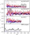 |
Fig. 1. Volume-averaged Toomre parameter, ⟨Q⟩, evaluated for simulations sg-mhd-tau10 (red) and sg-mhd-tau20 (blue). The vertical lines indicate the times at which the seed fields were introduced. |
Summary of all ideal-MHD simulations.
5.1. Simulations without background heating
In Löhnert & Peeters (2022), GI simulations with cooling and additional background heating (second term in Eq. (5)) were studied in which a small ZNF-type magnetic seed field was introduced into a fully GI-turbulent state. The runs, shown here, also introduce a initial-ZNF field, into GI turbulence, though now without additional background heating. The two main simulations are sg-mhd-tau20 and sg-mhd-tau10, with cooling times τcΩ0 = 20 and τcΩ0 = 10, respectively. sg-mhd-tau20 was restarted from the pure-GI simulation GI072 of Löhnert & Peeters (2022) at tΩ0 = 120. Simulation GI072 uses the full cooling law given in Eq. (5) with both heating and cooling and with a cooling timescale of τcΩ0 = 10. The averaged mass density in GI072 is such that the background speed of sound (cs, 0 = 1) is related to a background Toomre parameter of Q0 = 0.72. At the moment sg-mhd-tau20 is restarted from GI072 (tΩ0 = 120), the heating term (second term in Eq. (5)) was turned off, and the cooling time was set to τcΩ0 = 20. At first, B = 0, in order to achieve a new stationary GI state with the new cooling law. At tΩ0 = 200, the ZNF magnetic field is then seeded into the GI-turbulent state. Simulation sg-mhd-tau10 was restarted from sg-mhd-tau20 at tΩ0 = 200, but instead of introducing a seed field, the cooling time was reduced to τcΩ0 = 10. One might ask why sg-mhd-tau10 was not restarted from GI072 as well. It turns out that removing background heating at τcΩ0 = 10 can cause numerical instabilities; hence, first removing heating at tΩ0 = 20 and afterwards reducing the cooling time was the more reliable choice. In sg-mhd-tau10, the pure-GI state was then evolved until tΩ0 = 400. At that point, the ZNF field was introduced. In both sg-mhd-tau20 and 10, the ZNF-seed field is of the form  , with a field amplitude, B0, chosen such that ⟨β⟩xy = 107, at the mid-plane. More details about the numerical settings of these simulations are provided in Table 1. Additionally, a pure-MRI simulation, in the following referred to as MRI-compare, was set up, in order to provide a comparison. The latter is an isothermal simulation, that is, the equation of state is given by
  , where the isothermal sound speed, cs, i, was chosen such that
  . This choice is deliberate, in order to allow an easier comparison to the GI cases. We note that H-correction was not used here as it is not required and in fact caused numerical difficulties. The seed-field configuration is exactly equal to that of the GI cases, except that ⟨β⟩xy = 100, at the mid-plane. More details about the simulation parameters are provided in Table 1. Also shown in Table 1 is the ideal-MHD simulation sg-mhd-2, which is discussed in detail in Löhnert & Peeters (2022). The latter uses a cooling time of τcΩ0 = 10, but also includes background heating, second term of Eq. (5), with cs, 0 = 1, and a corresponding Toomre value of Q0 ∼ 0.75.
The time evolutions of the volume-averaged, dimensionless turbulent stresses, for simulations sg-mhd-tau20, sg-mhd-tau10, sg-mhd-2, and MRI-compare, are shown in Fig. 2. The stresses were calculated using Eqs. (8) and (9). We note that the factor γ, in Eq. (9), is also used for the isothermal MRI case, in order to retain comparability. In all GI cases, the vertical solid line marks the time point, at which the ZNF-seed field is introduced.
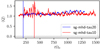 |
Fig. 2. Dimensionless stresses as a function of time for simulations sg-mhd-tau20 (τcΩ0 = 20), sg-mhd-tau10 (τcΩ0 = 10), sg-mhd-2 (τcΩ0 = 10, Q0 ∼ 0.75), and MRI-compare. Shown in blue is the Reynolds contribution, αr, in red the gravitational contribution, αg, and in black the Maxwell part, αm. All stresses were calculated using Eqs. (8) and (9), and the factor γ = 1.64 was also used for the isothermal MRI, allowing for an easier comparison. The curves for sg-mhd-tau20 and 10 start at tΩ0 = 120, at which point the simulations were restarted from the pure-GI state of GI072 (see Löhnert & Peeters 2022). Then, the cooling time was set to τcΩ0 = 20, and background heating was turned off (only cooling). At tΩ0 = 200, either one of two things happens, depending on the simulation. In sg-mhd-tau20, the ZNF field was introduced directly at tΩ0 = 200, highlighted by the solid vertical line. In sg-mhd-tau10, the pure-GI phase was prolonged from tΩ0 = 200 (vertical dashed line) to tΩ0 = 400 (vertical solid line), but the cooling time was reduced to τcΩ0 = 10. At tΩ0 = 400, the ZNF field was introduced. For both sg-mhd-tau20 and 10, the values of αg and αr were smoothed by convolving the respective time series with a Gaussian function (standard deviation σ = 3 |

After the introduction of the seed, the dimensionless Maxwell stress, αm, grows significantly, yielding values that are larger, or comparable to the remaining stresses. For the case with the longest cooling time (sg-mhd-tau20, τcΩ0 = 20), αm grows to become the dominant stress contribution. Contrary to that, the gravitational stress contribution, αg, decreases in all cases. The smallest changes occur to the dimensionless Reynolds stress, αr. All GI simulations require a considerable amount of time to saturate, ≳200 − 800  ; the τcΩ0 = 10 case appears to saturate the fastest. Volume- and time-averaged values, for the saturated phases of all runs, are provided in Table 1. One can then compare sg-mhd-tau20 and sg-mhd-2 at their initial phases with no or a vanishing magnetic field. It is apparent from Fig. 2 that the stress levels are comparable, despite sg-mhd-2 having a cooling time of τcΩ0 = 10 and sg-mhd-tau20 a cooling time of τcΩ0 = 20. Yet, this demonstrates the point, raised earlier, that additional heating can weaken GI, similar to a longer cooling time. The case with strongest GI is clearly sg-mhd-tau10, with the latter yielding a total stress, α, almost twice as large as the α-values obtained from the remaining simulations. In the dynamo-saturated phases, the Maxwell contributions are of equal magnitude for all GI simulations, αm = 0.0119, 0.0136, and 0.0092 for sg-mhd-tau20, 10, and sg-mhd-2, respectively. These values can be compared to the dimensionless Maxwell stress, observed in the pure-MRI simulation, αm = 0.0088. The GI values are consistently larger than the pure-MRI value; the largest deviation is observed for the strongest-GI case, sg-mhd-tau10. The deviations, relative to the pure-MRI value, are 5%, 35%, and 55%, for sg-mhd-2, sg-mhd-tau20, and sg-mhd-tau10, respectively.
It is also interesting to compare the pure-GI with the dynamo-saturated phases. The comparison is here provided for the simulations sg-mhd-tau10 and sg-mhd-tau20. The time intervals used for the initial and saturated phases as well as a selection of important, time-averaged values are shown in Table 2. The pure-GI phase (B = 0) of sg-mhd-tau10 exhibits significant oscillations. Hence, in order to obtain more reliable statistics, the GI-only state was prolonged from tΩ0 = 400, to 700; the corresponding time evolutions for α and ⟨Q⟩ are shown in Appendix A. The time average was then applied to the last 200 . One feature becomes immediately clear, the gravitational stress, αg, decreases significantly (from the GI-only to the dynamo-saturated state). The absolute reduction of αg is roughly equal for the two simulations. The total stress, α = αr + αg + αm, remains almost constant in comparison. In the dynamo-saturated state, the stress ratio, gravitational-to-Maxwell, αg/αm, is ∼0.56, for sg-mhd-tau20 and ∼1.35, for sg-mhd-tau10. Hence, in sg-mhd-tau20 the Maxwell stress dominates, whereas in sg-mhd-tau10 the gravitational stress is dominant. Since αm is almost equal in the two simulations, this reflects the fact that GI is stronger for τcΩ0 = 10, as compared to τcΩ0 = 20. Differences between sg-mhd-tau10 and 20, can also be seen in the time evolution of αm. In sg-mhd-tau20, at saturation, αm develops distinct oscillations, whereas sg-mhd-tau10 gives rise to more irregular αm-fluctuations. One can also compare the evolution of the Toomre values, from the GI-only to the saturated state. The Toomre value of sg-mhd-tau20 slightly increases, by roughly 10%. For sg-mhd-tau10, the saturation value slightly decreases by ∼8%. However, it has turned out that the exact value in the GI-only phase sensitively depends on momentary ⟨Q⟩ fluctuations. This can be seen in Fig. A.1, where the spike at the end of the averaging period leads to a significant contribution. If this spike is excluded, then the initial value is slightly smaller than the dynamo-saturated one. Hence, there is some statistical uncertainty in the exact values of ⟨Q⟩, for sg-mhd-tau10. A significant change in ⟨Q⟩, is not expected in any event, as GI saturates at marginal, gravitational stability, ⟨Q⟩∼Qc, with Qc ≳ 1. We note that this is also the case for all simulations, shown in Tables 1 and 2, and for both GI-only and the saturated phases. The time evolution of ⟨Q⟩ is shown in Fig. 1, for sg-mhd-tau10 (red) and sg-mhd-tau20 (blue). The vertical lines highlight the time points, at which the seed fields were introduced.
Comparison of the initial and saturated phases for simulations sg-mhd-tau20 and 10.
As discussed at the beginning of Sect. 5, it is this self-regulation to marginal stability, which necessitates a reduction of GI activity, as additional Maxwell stresses emerge. Hence, the reduction of αg in both simulations is in agreement with the simultaneous increase in αm. It is always possible that winds contribute to the overall energy balance. Whether winds are of importance can be tested, by comparing the stress values α, to the values αcool = 4/(9γ(γ − 1)τcΩ0) (see Eq. (10) and Gammie 2001). If wind losses were absent, a stationary turbulent state would require α = αcool. In the saturated phase, (α − αcool)/α ∼ 20% for sg-mhd-tau20 and ∼8%, for sg-mhd-tau10 (see Table 2). Yet, the Maxwell contributions are αm/α ∼ 47% for sg-mhd-tau20 and ∼30% for sg-mhd-tau10. Hence, the additional energy input, associated with αm, cannot completely be captured by wind cooling. Put differently, some of the additional energy input, associated with αm, contributes to heating. Regarding a possible GI-MRI coexistence, no definitive conclusion can be drawn, from α alone. One can say that sg-mhd-2 and sg-mhd-tau20 give rise to a similar, dynamo-saturated state, which is in agreement with the observation that the GI strength is roughly equal in the two cases. For the case with strongest GI activity, sg-mhd-tau10, the saturated state is qualitatively different from those of sg-mhd-tau20 and sg-mhd-2 in some aspects (e.g. more irregular αm-fluctuations, larger values of αg/αm). In Löhnert & Peeters (2022), it was argued that sg-mhd-2 is a state of GI-MRI coexistence. Hence, this suggests that stronger GI cases might lead to a qualitatively different saturation state of the dynamo.
As a further test, one can evaluate the vertical magnetic-field structure. Shown in Fig. 3 are zt diagrams of the horizontally averaged magnetic field component, ⟨By⟩xy, for simulations sg-mhd-2, sg-mhd-tau20, sg-mhd-tau10, and MRI-compare. The pure-MRI case develops an oscillating butterfly pattern, shortly after initialisation. Simulations sg-mhd-2 (see also Löhnert & Peeters 2022) and sg-mhd-tau20 develop a clearly visible butterfly diagram as well, but it takes several 100 to reach a stationary pattern. We note that the diagrams, seen in sg-mhd-tau20 and sg-mhd-2, differ in some aspects from the pure-MRI butterfly diagram. Most notably, in MRI-compare, the magnetic-field strength peaks at ∼2 H above (below) the mid-plane. In contrast to that, the GI-MHD cases sg-mhd-tau20 and sg-mhd-2 develop significant field strengths, also within |z|≤2 H. The field pattern for sg-mhd-tau10 is less regular than in the other cases. Near the mid-plane, ⟨By⟩xy can retain its polarity for over ∼200
 , whereas, away from the mid-plane, the field changes polarity more frequently. It is also noted that the irregular field reversals are very similar to those seen in the ideal simulation PL-ZNF-ideal, in Riols et al. (2021). A nonlinear cooling model was used in the latter simulation, and the exact cooling time might depend on temperature fluctuations. However, the effective timescale, τeff, evaluated for PL-ZNF-ideal in Riols et al. (2021) is also close to 10. Hence, for ⟨By⟩xy(z, t), qualitative differences arise between the weaker GI cases (sg-mhd-2 and sg-mhd-tau20) and sg-mhd-tau10. The former lead to a butterfly diagram with clearly visibly field reversals that bears similarities with the pure-MRI butterfly diagram. For the case with highest GI activity, sg-mhd-tau10, a clearly visible butterfly diagram is absent, and more irregular field variations are observed. This, in combination with the more irregular αm variations, suggests that sg-mhd-tau20 and 10 lead to two different saturated dynamo states: a weak-GI dynamo, which shares some characteristics with the pure-MRI dynamo and a strong-GI dynamo, which is qualitatively different, and where MRI may be absent.
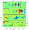 |
Fig. 3. Horizontally averaged toroidal magnetic field component, ⟨By⟩xy, as a function height, z, and time, t. The zt diagrams are shown for simulations sg-mhd-2, sg-mhd-tau20, sg-mhd-tau10, and MRI-compare. The time axis is chosen such that t = 0 corresponds to the moment of field seeding. |
One can directly check for sign reversals of ⟨By⟩xy, in the zt diagrams of both sg-mhd-tau20 and 10. This is demonstrated in Fig. 4, depicting sign(⟨By⟩xy), for sg-mhd-tau10 (first image) and sg-mhd-tau20 (second image). The mid-plane, in sg-mhd-tau10, can retain its polarity for extended periods of time, whereas frequent polarity reversals occur at higher altitudes. This state is similar to the intermediate regime, 100 ≤ tΩ0 ≤ 500, of sg-mhd-tau20. Differences arise at ∼600 , after field seeding, at which point the high-altitude oscillations form a coherent phase relation with the mid-plane field, in sg-mhd-tau20, magnetising the entire vertical extent of the disk. A similar phase locking does not occur in sg-mhd-tau10.
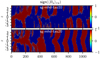 |
Fig. 4. Sign of the horizontally averaged toroidal magnetic field component. In this case, the “sign” has been intended to be a mathematical function, returning the sign of a value. sign(⟨By⟩xy), shown for simulations sg-mhd-tau10 and sg-mhd-tau20. The images can be directly compared to the corresponding zt diagrams in Fig. 3. |
Magneto-rotational instability is possibly absent, in sg-mhd-tau10, though, for now, this cannot definitively be decided. We note that more irregular field reversals have been observed in stratified, zero-net-vertical-flux MRI simulations (see e.g. Hirose et al. 2014; Coleman et al. 2017). There, vertical mixing, due to convection, prevents coherent sign reversals. It is not unreasonable that a similar, vertical mixing can be initiated by GI (see the horizontal rolls, above (below) density waves, in Riols & Latter 2018b). This may be related to the rather long time period (∼800 ), required to reach coherent ⟨By⟩xy oscillations, in sg-mhd-tau20, though the exact reasons for this are not entirely clear. To be sure, we checked whether accumulating, numerical errors have violated the ZNF condition, ⟨Bz⟩xy = 0, over time (see e.g. Silvers 2008), effectively leading to a net-flux case. However, it appears that this is not the case, and ⟨Bz⟩xy values are at most of the order of 10−9, or, in terms of a plasm β,
  .
.
Also evaluated are the volume-averaged plasma β, ⟨β⟩ = 2μ0P/|B|2, and the ratio of Maxwell stress to magnetic pressure, rsp = ⟨ − 2BxBy⟩/|B|2, for simulations sg-mhd-2, sg-mhd-tau20, 10, and MRI-compare. This is shown in Fig. 5, where ⟨β⟩−1 is depicted in the first image and rsp in the second image. The time axes are chosen such that t = 0 corresponds to the moment when the seed field is introduced. The plasma β saturates at values ⟨β⟩≳10 (see also Table 1), and this is true for both the pure-MRI case and the GI simulations. All cases settle into a state with rsp ≳ 0.3, and the saturation values are also robust in the sense that the fluctuations, with respect to the absolute values, are small in comparison. The value range 0.3 ≲ rsp ≲ 0.4 is shown to be typical for MRI, in a variety of studies (see e.g. Hawley et al. 1995, 2011; Blackman et al. 2008; Simon et al. 2011; Salvesen et al. 2016). Shortly after field seeding (for the first 100 to 200 ), the magnetic field strength is too low for MRI to be fully resolved (see also Löhnert & Peeters 2022), and only a pure-GI dynamo operates. The rsp values, evaluated in that period, are only slightly larger (rsp ≳ 0.4). Hence, this indicates that the initial, pure-GI dynamo also saturates at a roughly similar magnetic stress-to-pressure ratio. It is interesting that all simulations, including the MRI case, saturate at roughly the same ⟨β⟩ and rsp level, despite sg-mhd-tau20 and sg-mhd-tau10 leading to a qualitatively different dynamo appearance.
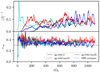 |
Fig. 5. Inverse volume-averaged plasma β, ⟨β⟩−1 = ⟨|B|2⟩/(2μ0⟨P⟩), and the ratio of Maxwell stress to magnetic pressure, rsp = ⟨ − 2BxBy⟩/(|B|2), as a function of time. The depicted simulations are sg-mhd-tau10 (red), sg-mhd-tau20 (blue), sg-mhd-2 (black), and MRI-compare (cyan). In all cases, the time t = 0 corresponds to the moment of field seeding. |
Finally, a visual representation of the saturated, turbulent state is provided in Fig. 6, for sg-mhd-tau20. Shown is the mid-plane mass density ρ(x, y), superimposed with magnetic field lines, traced in the (x, y) plane (only Bx and By are used for the tracing). The image was generated at tΩ0 = 1200. One observes a significant alignment of the field lines with GI-related density waves. A similar behaviour was also observed in Riols & Latter (2018a, 2019).
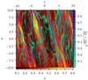 |
Fig. 6. Mid-plane mass density, ρ(x, y, z = 0), for simulation sg-mhd-tau20 evaluated at tΩ0 = 1200. The mass density is superimposed with magnetic field lines traced in the (x, y) plane with only the Bx and By components used for the tracing. |
5.2. Comparison to previous simulations
Löhnert & Peeters (2022) report differences to the previous comparable simulations provided in Riols & Latter (2018a), especially the τcΩ0 = 20 case, SGMRI-20, therein. The goal of this section is to single out the reason for the observed differences. In Löhnert & Peeters (2022), we argued that effects due to winds, crossing the vertical box boundaries, might have an influence on the simulation outcome. The corresponding simulation in Riols & Latter (2018a), SGMRI-20, uses a slightly smaller, vertical box size of 6 H, compared to our standard 8 H. We note that, due to the uncertainty of the exact value of cs in a turbulent state, an exact one-to-one comparison of box-sizes may be misleading. Hence, we provide a new simulation, sg-mhd-tau20-Lz6, with settings equal to run SGMRI-20 from Riols & Latter (2018a). Simulation sg-mhd-tau20-Lz6 is also listed in Table 1. All horizontal box dimensions are similar to the previous simulations, but the vertical box size is chosen to be Lz = 6 H, and the number of grid points is slightly increased to 500 per 20 H. This should provide a setup that is almost identical to SGMRI-20. Simulation sg-mhd-tau20-Lz6 is a completely new simulation and has not been restarted from any previous simulation. The simulation starts with a density and pressure distribution that is homogeneous in the horizontal directions (i.e. homogeneous across xy planes). In the vertical direction, a density and pressure stratification is established such that cs = 1 for all z. For the stratification equilibrium the contribution of self-gravity was included (see also the method in Löhnert & Peeters 2022). This initial state is perturbed by small, random deviations in both density and pressure (the deviation amplitude is 1% of the background value). The equilibrium is chosen such that ⟨Q⟩=csΩ0/(πG⟨ρ⟩Lz) = 1.0, at the start of the simulation. The simulation does not include background heating (no second term in Eq. (5)). Hence, cooling quickly causes the Toomre parameter, ⟨Q⟩, to drop below one. One then immediately observes the growth of GI; after ∼40 , the linear axisymmetric GI modes break up into non-axisymmetric turbulence. After ∼130
 , almost axisymmetric modes occur again, but they are less pronounced and quickly break up into GI turbulence again. The system then evolves into a stationary, turbulent state. The turbulent state is prolonged until tΩ0 = 200, where the ZNF magnetic field is seeded into the GI-turbulent state. The time evolution of the turbulent stresses is shown in the first image of Fig. 7. The two GI-break-up events at 40 and 130
 can be seen as the two spikes in the initial (GI) phase of the simulation. The seeding of the ZNF field is marked as the vertical dashed line (tΩ0 = 200). After seeding of the field, the behaviour of the stresses is very similar to that seen in sg-mhd-tau20. As αm increases significantly, the gravitational part αg drops, and αm eventually becomes the dominant contribution. And a butterfly diagram, equal to that of sg-mhd-tau20, also develops here, shown in the second image of Fig. 7.
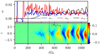 |
Fig. 7. Time evolution for a selection of quantities evaluated for sg-mhd-tau20-Lz6. First image: Dimensionless stresses as a function of time. Shown in blue is the Reynolds contribution, αr, in red the gravitational contribution, αg, and in black the Maxwell part, αm. All stresses were calculated, using Eqs. (8) and (9). The values of αr, and αg were smoothed using a Gaussian function (see also Fig. 2). Second image: Horizontally averaged magnetic field component, ⟨By⟩xy, as a function of height, z, and time, t. At tΩ0 = 200 (vertical solid line), the magnetic seed field is introduced. The vertical dashed line corresponds to 320 |

The reason for the differences is the amount of time required to reach a saturated state. In Riols & Latter (2018a), the stresses where evaluated for the first 320 , after the magnetic seed field was introduced. We, therefore, followed the same procedure and took a time average of the dimensionless turbulent stresses over the first 320
 after seeding of the field. This is done for sg-mhd-tau20-Lz6 and the previously discussed simulation, sg-mhd-tau20. The resulting stress values are provided in Table 3. We note that the stress values for SGMRI-20, obtained from Riols & Latter (2018a), have been multiplied by a factor 2/(3γ), in order to be consistent with the definition in Eq. (8). As one can see, the values are almost equal for all three simulations. Moreover, the zt diagram (second image of Fig. 7) for the first 320
 is very similar to that shown in Riols & Latter (2018a). One can therefore conclude that this is the reason why differences were observed in Löhnert & Peeters (2022). It is also noted that the zt diagram of the τcΩ0 = 10 simulation, SGMRI-10, shown in Riols & Latter (2018a), is qualitatively close to the more irregular field reversals seen in sg-mhd-tau-10 here. Hence, sg-mhd-tau10 is also compared to SGMRI-10 in the fourth and fifth rows of Table 3. One finds comparable values for the two simulations. Here, however, the average was taken over the saturated phase of sg-mhd-tau10. This is also reasonable as SGMRI-10 was restarted from SGMRI-20 and not completely run anew, indicating that it is perhaps closer to a saturated state. It appears that, at least for lower cooling times (weaker GI), one has to run simulations of the GI dynamo sufficiently long, in order to obtain the dynamo-transition to a defined butterfly diagram. We note that this is not an obvious point. The typical timescales for GI are of the order of the cooling time, here ∼10
 . Hence, it is surprising that the GI-MRI combined state requires ∼600
 to reach saturation. It is currently not clear why that is the case, and it is certainly an interesting question for upcoming research. However, as speculated in the previous section, this may be related to the time, required for the butterfly diagram to lock to the mid-plane field.
Dimensionless stress comparison.
5.3. Field generation
One can show that, in the local shearing box, the induction equation for the horizontally averaged fields (⟨Bx⟩xy, and ⟨By⟩xy) takes the following form (see e.g. Riols & Latter 2018a; Löhnert & Peeters 2022):
 (16)
(16)
 (17)
(17)
where ℰ = δv × B, is the electromotive force (EMF). This definition of ℰ does not distinguish between the averaged and the fluctuating field, whereas δv represents only the deviations from the shear flow. In the following, the vertical profiles of the field components and the EMFs are compared for simulations sg-mhd-tau20, 10, and MRI-compare. As one can see from the butterfly diagrams in Fig. 3, the horizontally averaged field components can change sign rather frequently. A direct time average leads to a cancellation, which is not desired. This can be circumvented by choosing a sign convention, before the time average is applied. If ⟨f⟩xy is a horizontally averaged dummy variable, depending on t and z, then the time-average is carried out as follows:
 (18)
(18)
This method certainly has caveats, since  must necessarily be positive for all z. The signs of
  ,
,  , and
, and  are always relative to By. However, one has to choose a height-dependent sign convention, as otherwise certain contributions would be lost. For example, in the zt diagram of sg-mhd-tau10, one can see that oscillations with a higher frequency occur for larger z values, but only a few field reversals are observed near the mid-plane. Choosing a fix sign for every time point would cancel out some contributions. However, applying the same averaging technique,
  , to all simulations still allows for a comparison of those simulations. The technique is first applied to simulation sg-mhd-tau20, and the resulting profiles are shown in Fig. 8. From top to bottom, the images show
  ,
,  ,
,  , and
, and  , respectively. The red line is a time average over the initial, weak-field phase (200 ≤ tΩ0 ≤ 400), and the blue line is an average over the saturated phase (800 ≤ tΩ0 ≤ 1300); the seed field is introduced at 200
 . For comparison, the same method is applied to the pure-MRI simulation, MRI-compare, and the resulting profiles are shown as the black, dashed curves. For MRI-compare, the time-average is over the 100 ≤ tΩ0 ≤ 1000 interval.
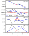 |
Fig. 8. Horizontally averaged field components and EMFs as a function of z. Solid curves correspond to sg-mhd-tau20, and dashed curves correspond to MRI-compare. The first two images depict ℰx, and ℰy, respectively. Images three and four show the magnetic field components Bx and By, respectively. The red curves were averaged over the 200 − 400 |


Considering the field components first, two features become immediately apparent, both components are mirror-symmetric with respect to z = 0, and in the initial phase the two field components are more localised near the mid-plane than in the saturated phase. In the initial phase, the toroidal component, By, is a decreasing function with |z|. In the saturated phase, By develops a dip at the mid-plane, which is not present in the initial profile. The radial component, Bx, changes sign, close to the mid-plane (|z|< 1 H), in the initial phase, which is also the case in the saturated phase. The two field components have in common that, in the saturated phase, significant field contributions arise at higher elevations, |z|> 1 H. The MRI does also lead to field contributions at higher altitudes, though there are qualitative differences to the saturated state of sg-mhd-tau20. Most notably, in MRI-compare, both field components have a distinct peak at |z|∼2, which is not the case for the sg-mhd-tau20 profiles, showing a more monotonous z dependence. Regarding the EMFs, the latter are, as expected, anti-symmetric with respect to the mid-plane. At saturation, a significant ℰx contribution arises for higher altitudes. And one can see that, for |z|≳1 H, ℰx is in agreement with the pure-MRI case. However, at the mid-plane, |z|≲1 H, ℰx is almost equivalent to the initial case. We note that ∂z⟨ℰx⟩xy corresponds to the rate of change, of ⟨By⟩xy. Hence, from the image, one can tell that the vertical derivative must change sign, from higher altitudes to the mid-plane region. This is in agreement with the dip (at the mid-plane), observed for By. However, we note that, due to the averaging technique, an exact sign comparison of the EMFs and fields may be misleading. For ℰy, a similar behaviour is observed. The initial phase only develops contributions near the mid-plane. In the saturated phase, the observed ℰy profile approaches that seen in the pure-MRI case, though superimposed with significant noise. Taken together, one can conclude that the saturated phase, of sg-mhd-tau20, is not inconsistent with a coexistence between GI and MRI. This is best represented by the ℰx component, which definitively shows characteristics of the initial (GI) phase near the mid-plane and characteristics of the pure-MRI case for higher altitudes. The field components in the saturated phase of sg-mhd-tau20 lack the field-strength peaks seen for the pure-MRI case, though. Yet, one can still observe that the saturated state of sg-mhd-tau20 gives rise to additional field contributions, at higher altitudes, which are less pronounced in the initial phase.
The same method is then applied to the strong-GI case, sg-mhd-tau10. Fig. 9 shows both the initial weak-field phase, 200 after field seeding (red), and the saturated phase, 1000 ≤ tΩ0 ≤ 1500 (blue). There are similarities to the sg-mhd-tau20 case, though there are also significant differences. Considering the field components first, one can see that the initial profiles are qualitatively similar to those seen in sg-mhd-tau20. The field profiles at saturation are much closer to the initial profile, than is the case in the weaker-GI simulation, sg-mhd-tau20. One can still see that saturation gives rise to additional field contributions, at |z|∼1 − 2, though they are less pronounced and certainly far from the field-strength peaks observed in the pure-MRI case. For the EMFs, one finds that, near the mid-plane, the ℰx profile almost does not change, from the initial to saturated phase. For higher |z|, saturation gives rise to larger ℰx values, though they do not reach the pure-MRI level. The toroidal component (ℰy) is different from the pure-MRI case and significantly dominated by noise.
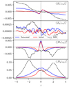 |
Fig. 9. Horizontally averaged field components and EMFs as a function of z, equivalent to Fig. 8 except now evaluated for simulation sg-mhd-tau10. Red curves are averages over the 400 − 600 |


Hence, the EMF analysis also suggests that there are two, qualitatively different ideal-MHD dynamo states: a (1) weak-GI state that is consistent with additional MRI contributions (GI-MRI coexistence) and (2) a strong-GI dynamo with significant mid-plane contributions and possibly no MRI. In the strong-GI case, the initial, weak-field phase is also similar to the dynamo-saturated state.
5.4. Exchange between magnetic and kinetic energy
In the local shearing box approximation, the magnetic energy balance can be written as follows (see also Brandenburg et al. 1995):
 (19)
(19)
The term ∂tEmag, on the left hand side, represents the net rate of change, of the volume-averaged magnetic energy density. The terms on the right hand side represent the causes for that change. The first term, (3Ω0/2)⟨ − BxBy/μ0⟩, is written as a volume average, though it really originates from a boundary integral, that is, from the divergence of the Poynting flux. Hence, this term represents the rate, at which energy enters (leaves) the box through the horizontal boundaries. This is similar to the kinetic energy balance, which has a contribution (3Ω0/2)⟨ρvxδvy⟩. In the global picture, this corresponds to the energy, locally released by the accretion process. The second term, ⟨(v × B)⋅J⟩, is the volume-averaged exchange rate, between the magnetic and kinetic energy budgets. We note that v is the actual velocity, containing both the shear flow and all perturbations. The third term, Fz, accounts for all losses of magnetic energy, over the vertical boundaries. The last term measures the rate at which magnetic energy is lost, due to resistive dissipation. The analytical form of ⟨η|J|2⟩ represents Ohmic dissipation, though even in ideal-MHD cases, dissipation can still occur at the grid scale, and, in conservative codes, this energy enters the thermal budget implicitly. We then analysed the terms ⟨(v × B)⋅J⟩ and (3Ω0/2)⟨ − BxBy/μ0⟩ for MRI-compare and sg-mhd-tau20 as a function of time. The result is shown in Fig. 10.
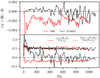 |
Fig. 10. Magnetic energy fluxes as a function of time evaluated for both sg-mhd-tau20 (black curves) and MRI-compare (red curves). Shown in the first image is the conversion rate from magnetic to kinetic energy, ⟨(v × B)⋅J⟩. This rate was calculated using the central differences from the full three-dimensional output data every 10 |

Shown in the first image are the volume-averaged kinetic-magnetic exchange rates, ⟨(v × B)⋅J⟩. A special feature of MRI is that the latter yields values smaller zero. This has already been observed in early simulations of MRI (see Brandenburg et al. 1995). At first, this may seem counter-intuitive as one would expect a dynamo to turn kinetic energy into magnetic energy, and not vice versa. For the cases here, this is not a contradiction, and the energy input is actually related to (3Ω0/2)⟨ − BxBy/μ0⟩ (see below). First, one can analyse the same exchange rate for sg-mhd-tau20, shown as the solid black line in the first image. During the initial phase, the exchange rate appears to be positive, on average. However, at later times, starting at tΩ0 ∼ 750, the exchange rate turns negative, similar to the pure-MRI case. This raises the questions as to where the magnetic energy is coming from in the first place and how the negative exchange rate should be interpreted since GI seems to provide a dynamo. Here, the dominant input of magnetic energy originates from the contribution of the Maxwell stress, 3Ω0⟨−BxBy⟩/(2μ0). To put this into perspective, both 3Ω0⟨−BxBy⟩/(2μ0) and ⟨(v × B)⋅J⟩ are shown in the second image. All values were normalised by the momentary value of Emag, as this allows a direct comparison of the initial and saturated phases. We note that, normalised by Emag, the stress contribution is essentially (3Ω0/2) rsp. Hence, this demonstrates explicitly that rsp yields exactly equal values in the GI-MHD state and in the MRI state. It becomes clear that, in the saturated phase of sg-mhd-tau20 and in the pure-MRI case, the term 3Ω0⟨−BxBy⟩/(2μ0) represents the dominant energy input. Hence, the energy input actually originates from the stresses. However, during the initial phase of sg-mhd-tau20, one finds ⟨(v × B)⋅J⟩> 0, which is in agreement with the proposed GI dynamo. After ∼250 , the values ⟨(v × B)⋅J⟩ gradually approach zero, on average. This is not entirely unexpected, as the GI dynamo must eventually saturate. However, the question remains as to why this exchange rate eventually turns negative, after tΩ0 ∼ 750. In the case of MRI, this may be understood as a consequence of the instability mechanism itself. In the ideal-MHD limit, the presence of a sub-thermal magnetic field is sufficient to induce MRI (see e.g. Balbus & Hawley 1998). Without that field, no instability occurs. In the context of a dynamo, MRI is special, as Lorentz forces are important from the very start. Put differently, MRI must not only sustain its own field, it must also sustain its own turbulence via Lorentz forces (see Balbus & Hawley 1998). Hence, it is not unreasonable to find ⟨(v × B)⋅J⟩< 0, as, in the case of MRI, Lorentz forces are the primary cause why fluid elements move in the first place. This suggests that some type of mechanism capable of generating kinetic energy from magnetic energy must also be present in sg-mhd-tau20. Magneto-rotational instability would provide such a mechanism, and this falls in line with the butterfly diagram, as well as the vertical EMF profiles.
5.5. Interpretation and summary
Considering all previous simulations, one can conclude that there appear to be two different dynamo states, associated with GI, in an ideal-MHD regime. A weak-GI case, which shares similarities with the MRI dynamo and a strong, possibly pure, GI state. All regimes have in common that the gravitational stress contribution, αg, decreases significantly, as the Maxwell stress, αm, increases. Simulation sg-mhd-tau20 offers a good reference point for a closer inspection. In sg-mhd-tau20, αg decreases by more than a factor of two, from the GI-only phase (160 − 260 ), to the dynamo-saturated phase (800 − 1300
 ) (see also Table 2). GI-only here means that B = 0 or at least negligible (the seed field is introduced at tΩ0 = 200). The volume-averaged Toomre parameter, ⟨Q⟩, increases slightly, by ∼10%. In sg-mhd-tau20, the total mass and the cooling time are held constant and no additional heating (second term in Eq. (5)) is used. Hence, one can ask how GI activity is actually reduced. Clearly, some back-reaction, via Lorentz forces, must occur. For example, one might take into account the stabilising effect of magnetic pressure forces. Considering the magnetic pressure in the definition of the Toomre parameter (see e.g. the approach in Riols & Latter 2019), one finds
  , which, for ⟨β⟩ = 12 (see Table 1), yields an increase of
  . The increase by thermal means alone, is already at ∼10%, and hence, if pressure forces are responsible for the GI reduction, then thermal pressure forces are the dominant contribution. A back-reaction can also occur via field-line bending forces ∝(B ⋅ ∇)B.
The xy components, of these bending forces, are compared to the xy components of the self-gravity forces, for sg-mhd-tau20, in Fig. 11, where the absolute values of the force densities were averaged horizontally and over time (800 − 1300  ). At the mid-plane, self-gravity forces in the x direction are stronger by a factor of ∼7.8, and in the y direction by a factor of ∼1.8. Hence, the radial motions should be largely unaffected. One could argue that motions in the y direction are affected, by field-line bending forces. However, one has to keep in mind that GI saturation is induced by thermal self regulation. Heat, generated by GI itself, brings the system to the instability threshold ⟨Q⟩∼Qc. If a non-thermal force, such as field-line bending, was to contribute to GI saturation, then GI does not saturate by thermal means alone. In fact, as GI is weakened, producing less heat, one would actually expect a lower ⟨Q⟩ value. The question thus remains as to how GI activity is reduced. In light of the previous findings, we suggest that the mechanism of GI weakening is related to a coexistence with MRI, at least in sg-mhd-tau20. How this can be achieved is discussed at the beginning of Sect. 5. The mechanism of MRI leads to an additional energy input. The latter cannot completely be captured by wind losses, and some parts must contribute to heating. However, in the presence of GI, the thermal energy level cannot rise indefinitely, as GI-turbulent states self-regulate to marginal stability, ⟨Q⟩∼Qc, with Qc ≳ 1 (see e.g. Gammie 2001). Significantly larger ⟨Q⟩ values result in a GI-stable configuration. Hence, the additional energy production rate, due to MRI, enforces a reduced energy production rate, due to GI, in order to sustain ⟨Q⟩∼Qc. This is not to say that ⟨Q⟩ cannot increase, it only means that ⟨Q⟩ cannot increase by much (e.g. 10% for sg-mhd-tau20). Moreover, from Fig. 11, one can deduce that field line bending forces dominate over self-gravity forces, above |z|∼2 H. This is also where the highest field strengths were observed, in the pure-MRI case. The mechanism of MRI is indeed based on the bending of field lines and, in combination with differential rotation, is capable of drawing free energy from the background flow. Put differently, it is not so much a direct back-reaction of Lorentz-forces that causes a reduction of GI activity, but rather the fact that a positive correlation ⟨ − BxBy⟩ is established. The latter leads to a net input of magnetic energy, which, at least in parts, must contribute to heating. This, in combination with the ⟨Q⟩∼Qc requirement, necessitates a reduction of GI activity (see also Sect. 5).
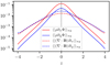 |
Fig. 11. Absolute values of the field line bending forces, ⟨⟨|(B ⋅ ∇)Bx, y|⟩xy⟩t (solid curves), and the self-gravity forces, ⟨⟨|ρ∂x, yΦ|⟩xy⟩t (dashed curves), in directions x (red) and y (blue), evaluated for simulation sg-mhd-tau20. The time average is over the interval 800 ≤ tΩ0 ≤ 1300. The force densities were calculated using finite differences from the full three-dimensional output data of Athena every 10 |

We note that each diagnostic, on its own, cannot definitively proof the presence of MRI, in the dynamo-saturated state. However, one has to consider the net of all diagnostics, and the latter suggest a form of GI-MRI coexistence, in the weak-GI case, sg-mhd-tau20. And the presence of MRI can explain the observed reduction of GI activity. We note that the exact mechanisms leading to saturation in the strong-GI simulation, sg-mhd-tau10, are less clear, and MRI is possibly absent. However, also in sg-mhd-tau10, an additional αm contribution arises, and the energy balance has to account for that, MRI or not. Finally, one also has to distinguish between a turbulence and a dynamo mechanism. Magneto-rotational instability alone has to sustain both, as the turbulence mechanism requires a field to operate on. One might even speculate whether GI is beneficial for MRI, as GI can sustain a background field for the MRI to operate on. But we acknowledge that the definitive mechanism for how the ideal GI dynamo saturates is still elusive.
6. Including resistivity, a new nonlinear state
As discussed in the previous sections, additional, turbulent energy production (e.g. due to MRI) can cause GI to weaken, given that the cooling physics does not change. Thereby, the excess-energy input can effectively act as an additional heating source. The additional heat may arise from the dissipation of kinetic energy (e.g. generated by MRI), or by dissipation of magnetic energy at the grid scale, which is implicitly turned into thermal energy via energy conservation. Considering the last point, it is worth to introduce explicit Ohmic dissipation, in order to test the influence of magnetic heating on GI, by resolving the magnetic dissipation at small scales. The first resistive simulation presented here is sg-eta01. The latter is restarted from the ideal-MHD simulation sg-mhd-2, at tΩ0 = 1000, but with a finite resistivity value, being introduced at the moment of restart. Simulation sg-mhd-2 is discussed in Sect. 5.1 and in more detail in Löhnert & Peeters (2022). As can be seen in Fig. 3, sg-mhd-2 develops a clearly visible butterfly diagram. The value of Ohmic resistivity, in sg-eta01, is η = 0.01. Using the background value of the sound speed, cs, 0 = 1.0, then this corresponds to a magnetic Reynolds number of Rm = 100 (see Eq. (13)). However, using the volume- and time-averaged sound speed, ⟨⟨cs⟩⟩t, one finds a larger value of ⟨⟨Rm⟩⟩t ∼ 281. A detailed list of the simulation parameters to sg-eta01 is provided in the first line of Table 4. The total mass content in the box volume is held constant via the replenishing method, detailed in Sect. 4.1. As sg-eta01 was restarted from sg-mhd-2, it also includes background heating (second term in Eq. (5)). Without turbulence, the balance of heating and cooling would cause a state with a constant normalised sound speed of cs, 0 = 1, which corresponds to a Toomre parameter of Q0 ∼ 0.75, given the constant box mass. In the following, we show that this value of resistivity leads to a new turbulent state that differs from the ideal-MHD states shown so far, particularly the GI-MRI coexistence states. Hence, a new saturation mechanism is established, which, considering the uncertain case sg-mhd-tau10, possibly provides a third dynamo state.
Scan over different values of η.
6.1. Observed time evolution
Shown in the first image of Fig. 12 is the time evolution of the dimensionless turbulent stresses αr (Reynolds), αm (Maxwell), and αg (gravitational). The time before tΩ0 = 1000 corresponds to simulation sg-mhd-2 (see Sect. 5.1 and Löhnert & Peeters 2022), and the time afterwards is sg-eta01, with resistivity being enabled at the transition. The values of both αg and αr were smoothed, by convolving the respective time series with a Gaussian function with standard deviation σ = 3 . Directly after enabling resistivity, the Maxwell stress αm drops significantly, whereas the gravitational and Reynolds stresses remain mostly unchanged. However, αm immediately enters a growth phase, growing even larger than the initial, non-resistive value at tΩ0 ∼ 1200. At that point, the gravitational stress αg is dropping significantly. Eventually, αm and αg reach a maximum and a minimum, respectively. The gravitational stress then recovers to the previous value. At tΩ0 = 1500 the stresses are similar to the state at tΩ0 = 1200 and the process repeats. Hence, the system settles into a new nonlinear state, with effective oscillations occurring in both αg and αm. During the oscillations, it is apparent that the Reynolds stress remains relatively constant, with only small spikes occurring during maxima in αg.
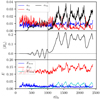 |
Fig. 12. Time evolutions for a selection of volume-averaged quantities evaluated for sg-eta01. First image: Turbulent stresses αr (Reynolds), αm (Maxwell), and αg (gravitational) as a function of time. The values for both αg and αr were smoothed by convolving the respective time series with a Gaussian function and with a standard deviation of σ = 3 |

The second image in Fig. 12 depicts the volume-averaged toroidal magnetic field component ⟨By⟩ as a function of time. For tΩ0 < 1000 (ideal-MHD phase, sg-mhd-2), one can clearly observe the field oscillations indicating the butterfly diagram, detailed in Löhnert & Peeters (2022). After resistivity is enabled at 1000 , the oscillation is disrupted, and for tΩ0 ≳ 1300 a new oscillating state develops, but with the oscillations now centred around a finite, positive ⟨By⟩. It is also easily seen that the averaged field strength is significantly larger in the newly developed nonlinear state. In Löhnert & Peeters (2022), we remarked that the periodically occurring field reversals are a distinguishing feature from the findings in Riols & Latter (2018a), where field oscillations occur less regularly. In the resistive cases in Riols & Latter (2019), field reversals are even absent completely. Hence, these findings might be more reminiscent of the case sg-eta01 studied here. The oscillatory behaviour can also be observed in the volume-averaged energy densities (see the third image of Fig. 12). At each time point, the energy densities are obtained using Eqs. (11a)–(11c). At tΩ0 ∼ 1200, the magnetic energy density is equal in magnitude to the kinetic energy density and is continuing to grow. Similar to αm, also Emag eventually reaches a maximum value and oscillates from then on. The oscillations are also observed for the thermal energy density Eth. The kinetic energy density Ekin remains almost constant from 1200
 onwards, with only short fluctuations occurring. The latter fluctuations (short spikes in Ekin) seem to solely appear during minima in the magnetic energy Emag.
Shown in Fig. 13 is a (z, t) diagram of the horizontally averaged, toroidal magnetic field component, normalised by the root-mean-squared (rms) value,  . Most notably, the butterfly pattern, occurring during the ideal phase, is disrupted, after resistivity is enabled. A field modulation still occurs (see also the second image of Fig. 12), but the clearly visible field reversals are absent. Finally, in Fig. 14, the mid-plane mass density, evaluated at tΩ0 = 2000, is superimposed with magnetic field lines, traced in the (x, y) plane. Similar to Fig. 6, the field lines are mostly aligned with the GI density waves, but, in contrast to the ideal-MHD cases, the field lines develop fewer small-scale structures. In Fig. 6, one can see that, especially in the regions between density waves, the field lines change direction rather frequently. This is not the case in Fig. 14, and the field lines bridge the gap between density waves more straightly.
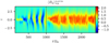 |
Fig. 13. Vertical profile of the normalised, horizontally averaged magnetic field component, |
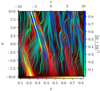 |
Fig. 14. Mass density at z = 0 and tΩ0 = 2000 for simulation sg-eta01. The image is overlayed with magnetic field lines traced in the (x, y) plane and only using the field components (Bx, By). |
Considering the previous findings, it becomes clear that the new nonlinear state, after enabling resistivity, is qualitatively different from the ideal-MHD state. The aim of the following section is to elucidate the physical mechanisms of this new, nonlinear state.
6.2. Saturation mechanism
It is clear from the first image of Fig. 12 that oscillation maxima in the Maxwell stress, αm, correspond to minima in the gravitational stress, αg, and vice versa. During minima, the gravitational stress is reduced to almost zero. As can be seen in Fig. 15, the oscillations also occur for the volume-averaged Toomre parameter (red curve), and maxima of ⟨Q⟩ correspond to minima in αg.
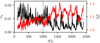 |
Fig. 15. Time evolution of the volume-averaged Toomre parameter, ⟨Q⟩ (red curve), and the dimensionless gravitational stress, αg (black curve), evaluated for sg-eta01. The vertical dashed line at tΩ0 = 1000 marks the time point at which resistivity is introduced. The αg values were smoothed using a Gaussian function with standard deviation σ = 3 |

These oscillations, in the Toomre values ⟨Q⟩, are close to those observed in the resistive simulations of Riols & Latter (2019) and the ambipolar diffusion simulations in Riols et al. (2021). There, it is suggested that changes in both the magnetic and the thermal pressure might cause changes in Q. The magnetic pressure increases as the GI dynamo generates magnetic energy, and the thermal energy increases due to resistive dissipation of magnetic energy. The increased Toomre parameter is then related to a weaker GI, corresponding to lower αg values. One usually expects the stress α to be determined by the cooling time alone (see Gammie 2001). However, as pointed out earlier, additional heating can also reduce the strength of GI, even for a given cooling time (see e.g. Rice et al. 2011). This may lead to a slightly larger Toomre value, ⟨Q⟩, though this increase is usually small, as a GI-turbulent state saturates at marginal stability ⟨Q⟩∼Qc, with Qc ≳ 1. Significantly larger values indicate stability against GI and are not compatible with a GI-turbulent state. As can be seen in Fig. 15, the increase in ⟨Q⟩ is rather significant, up to values of ⟨Q⟩∼1.4. An those maxima correspond to drops in αg, to almost zero. As the mass density is held constant, one can infer that some form of heating arises that is significant enough to render the system almost gravitationally stable.
The question then arises as to how the excess thermal energy, which increases the Toomre parameter, is produced. Here, thermal energy can change due to radiative cooling (heating), conversion of kinetic energy via compression (expansion), conversion of magnetic energy due to Ohmic resistivity, and fluxes across the vertical boundaries. From the first image in Fig. 12, one can immediately conclude that the thermal energy density Eth is correlated with the oscillations in the magnetic energy density Emag, whereas the kinetic contribution remains almost unchanged. This suggests that the resistive dissipation of magnetic energy is causing the oscillations in the thermal energy density and subsequently the oscillations in ⟨Q⟩. To test this, one can analyse the energy balance in the resistive state, in more detail. For this, the volume-averaged, resistive dissipation rate, ⟨η|J|2⟩, is calculated explicitly, as a function of time. One would then expect to find oscillations in ⟨η|J|2⟩ as well. This is indeed the case, as can be seen in Fig. 16, which shows the net cooling rate, according to Eq. (5), with cs, 0 = 1. The latter depends directly on Eth and, therefore, also develops oscillations. One notices that the oscillations of the resistive dissipation rate, ⟨η|J|2⟩, and the oscillations of the cooling (heating) rate are of the same order of magnitude, which indicates that resistive dissipation is indeed responsible for the periodically occurring heating events. The curves do not fit exactly though, and the cooling (heating) rate  is always larger than ⟨η|J|2⟩. The difference originates from the remaining thermal energy production via dissipation of turbulent kinetic energy. However, the oscillations occurring in both ⟨η|J|2⟩ and
  are in good agreement. Observing Fig. 16 closely, one also notices that ⟨η|J|2⟩ and
  are slightly out of phase, with ⟨η|J|2⟩ slightly leading. That is reasonable since ⟨η|J|2⟩ really needs to increase first, before the thermal energy, and with it the cooling rate can rise.
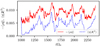 |
Fig. 16. Negative cooling (heating) rate ( |


Additionally, one can analyse the magnetic energy balance, according to Eq. (19), for sg-eta01. Shown in Fig. 17 is the time evolution of the terms (3Ω0/2)⟨ − BxBy/μ0⟩, ⟨v × B ⋅ J⟩, and ⟨ − η|J|2⟩. All values were normalised by the momentary values of Emag, that is, all rates are in units of Ω0. The time before tΩ0 (vertical, dashed line), corresponds to the ideal case sg-mhd-2, and the resistive phase of sg-eta01 starts immediately after that time. The Ohmic dissipation, ⟨ − η|J|2⟩, is only shown for the resistive phase. We note that, in Code units (Ω0 = 1), the Maxwell-stress contribution is essentially given by 1.5 rsp. In the ideal phase of sg-mhd-2, the time evolution of ⟨v × B ⋅ J⟩ (blue curve) is similar to that of sg-mhd-tau20, detailed in Sect. 5.4. Directly after field seeding, the values are positive, and kinetic energy is converted into magnetic energy. In the saturated, ideal phase (GI-MRI coexistence ∼700 − 1000 ), the values are, on average, negative (see also the discussion in Sect. 5.4). During the ideal phase, most of the energy input arises from the stress contribution, 1.5 rsp. Time-averaged over the 700 − 1000
 interval, one finds rsp = 0.34 (see Table 1). As resistivity is enabled, the values of rsp drop significantly, leaving the MRI-typical range rsp ≳ 0.3. Time-averaged over the 1300 − 2400
 interval, one finds rsp = 0.17 (see Table 4). It is again noted that all values, shown in Fig. 10 are normalised by Emag. The absolute values of Emag and αm increase as resistivity is enabled (see Fig. 12). However, the ratio rsp = ⟨ − BxBy/μ0⟩/Emag decreases. From dimensional grounds one can say that ⟨ − BxBy/μ0⟩ scales with the magnetic energy. Hence, whatever generates the additional magnetic energy, in the resistive phase, is related to a comparatively smaller Maxwell stress, as compared to the ideal phase. Similarly, the relative importance of ⟨v × B ⋅ J⟩ drops. This is consistent with the suppression of MRI, once resistivity is enabled. Moreover, one can see that most of the energy input, arising from 1.5 rsp, is thermalised by Ohmic dissipation, ⟨ − η|J|2⟩ (red curve). This demonstrates that most of the magnetic energy production is passed through to thermal energy, which is in agreement with the significant heating.
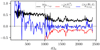 |
Fig. 17. Contributions to the magnetic energy balance evaluated for sg-eta01 as a function of time. All values are normalised by the momentary magnetic energy density, Emag. Shown in blue is the volume-averaged rate at which magnetic energy is converted to kinetic energy, ⟨v × B ⋅ J⟩. The values were calculated from the full three-dimensional output data using central differences every 10 |


The previous findings point to a possible process for nonlinear saturation. The causal steps leading to one oscillation are reminiscent of those proposed in Riols & Latter (2019) and are outlined in more detail below. As resistivity is enabled, the previous saturation mechanism (possibly MRI) fails and the GI dynamo continues to produce net-magnetic flux, ⟨Bx, y⟩, as well as magnetic energy, Emag. As the magnetic energy density increases, the resistive dissipation rate also increases. The latter leads to heat production ⟨η|J|2⟩ and, consequently, an increasing thermal energy density, Eth. The excess thermal energy, in turn, causes an increase in the saturated Toomre parameter ⟨Q⟩, which corresponds to a significantly reduced GI activity. The reduced (almost vanished) GI means that the dynamo is also weakened and the magnetic energy increase stagnates, reaching a maximum. In consequence, resistivity leads to the decay of remaining, excess magnetic energy. With the decreasing magnetic energy, the resistive heat production is also decreasing. Eventually, the system cools to its original state, yielding a minimum in both the thermal energy level and the magnetic energy level. At that point, GI can reignite turbulence. One might speculate that this reignition causes the short spikes in the kinetic energy, Ekin, occurring during minima of Emag (see the third image of Fig. 12). The revived GI also reignites the dynamo and the magnetic energy starts to increase again, starting a new cycle. Due to the nature of this cycle, we refer to this new nonlinear state in the following as ‘resistive-GI dynamo’. We note that Riols et al. (2021) found similar results for MHD simulations of GI with ambipolar diffusion instead of Ohmic resistivity. There, oscillations in ⟨Q⟩ were also observed. Furthermore, Riols et al. (2021) also tested a nonlinear cooling law, of the form  (τ0=const.), and claim that this does not lead to oscillations. Finally, the magnetic Reynolds number Rm = 100 lies in the range of values, studied in Riols & Latter (2019). Hence, one might speculate that, for GI-MRI coexistence, the Rm values need to be significantly larger than 100.
6.3. Timescales
The previous discussion suggests that one might distinguish between three different dynamo regimes: two ideal-MHD states (GI-MRI coexistence, with weak GI and a strong-GI dynamo) and the resistive-GI dynamo. The goal of this section is to obtain estimates for the dynamo growth rates. We distinguish between the ideal-MHD growth rates and the resistive growth rates. The ideal-MHD simulations, for which the field growth was evaluated, are sg-mhd-tau10, sg-mhd-tau20, and sg-mhd-2. The evaluation was also applied to simulation sg-eta01, though here, the growth rate was measured for the interval after resistivity was enabled (1000 ≲ tΩ0 ≲ 1300). The growth rates were calculated, by evaluating the time evolution of the volume-averaged magnetic energy density, Emag. This is shown in Fig. 18, where the ideal simulations sg-mhd-2, sg-mhd-tau10, and 20 are shown along with the resistive case, sg-eta01. The time axis starts at zero for all simulations. For the ideal cases, t = 0 corresponds to the seeding of the field, whereas for sg-eta01, it corresponds to the introduction of Ohmic resistivity. The plot for Emag is logarithmic, and growth phases can be identified as phases with almost linear increase in log(Emag). These are shown for each simulation as the dashed black lines. The corresponding time intervals are provided in Table 5. To avoid artefacts of the initial state, all intervals start 10 after seeding, or introduction of resistivity. Assuming the magnetic energy grows exponentially (Emag ∝ exp(g t)), the growth rates g can be determined from the linear slopes m, in Fig. 18, via g = m/log10e. The resulting values are provided in Table 5. In addition to the growth rates, the resistive damping rates were also evaluated for two decay phases of sg-eta01, shown in the last two rows. The corresponding linear trends are depicted as the dotted lines in Fig. 18. We note that the growth rates were determined here with respect to the magnetic energy density. Since the latter scales quadratically with the magnetic field strength, the growth rates, evaluated for the actual field strength, can be lower by a factor of two.
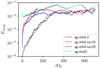 |
Fig. 18. Volume-averaged magnetic energy density, Emag, for the ideal-MHD simulations sg-mhd-2 (black), sg-mhd-tau10 (red), and sg-mhd-tau20 (blue) and the resistive simulation sg-eta01 (cyan). The time axis starts at t = 0 for all simulations. For the ideal-MHD runs, this corresponds to the moment of field seeding and for the resistive run, (t = 0) corresponds to the moment when resistivity was introduced. The dashed black lines correspond to linear fits, according to the values in Table 5. |
Growth and damping rates for each simulation.
For the ideal-MHD cases, the lowest growth rate (g = 0.0346) was determined for sg-mhd-tau20, which corresponds to the largest cooling time of τcΩ0 = 20. However, the value for the τcΩ0 = 10 case (g ∼ 0.0415) is only slightly different, despite using a twice shorter cooling time. The largest growth rate was determined for the heated case, sg-mhd-2 (see also Löhnert & Peeters 2022). We point out, though, that the selection of time intervals used to calculate the growth rates is a matter of choice and that, especially for sg-mhd-tau10 and 20, there is some ambiguity. Also, the ideal growth rates do not deviate by much and are all roughly consistent with gi ∼ 0.04. Hence, whether definitive trends can be derived from this is questionable. However, one can clearly see that the ideal growth rates are larger (by roughly a factor of three to four) than the resistive growth rate (gr ∼ 0.013), obtained for sg-eta01, in the initial growth phase after the introduction of resistivity. Additionally, the damping rates were calculated, by evaluating the negative slopes (see the dotted lines in Fig. 18). The corresponding values are provided in the last two lines of Table 5. The two decay phases lead to two differing values, gd = 0.014 and 0.0338, with a mean value of gd = 0.0244. We note that this value is roughly equal to the difference between the ideal and the resistive growth rate, gi − gr ∼ 0.027.
However, the original two damping rates deviate rather substantially, and this may well be a coincidence. However, one important feature of the resistive state is that the magnetic energy increases in the first place as resistivity is enabled. This may point to a slow dynamo process whereby resistivity is actually beneficial for the GI dynamo (see also Riols & Latter 2019).
Finally, one can also compare the growth rate obtained for the resistive state with the growth rates found in the resistive simulations of Riols & Latter (2019). The latter find, for a case with τcΩ0 = 20 and Rm = 200, a growth rate of g ∼ 0.028Ω0. This can best be compared to our simulation sg-eta01, as the latter yields a volume-averaged magnetic Reynolds number of ⟨⟨Rm⟩⟩t ∼ 280. For the latter, the obtained growth rate is ∼0.013 (see Table 5). Hence, the values clearly have the same order of magnitude, though they are not equal. However, we note that there is some ambiguity, regarding the exact values of Rm, as the latter can strongly depend on the exact choice of the sound speed cs (mid-plane, volume-averaged, initialisation value, etc.). Also, the cooling time used in sg-eta01 is only half as long (τcΩ0 = 10). Comparing, instead, the growth rate for the ideal run sg-mhd-tau20 (g ∼ 0.0346), one recovers a slightly larger value, than that seen in Riols & Latter (2019). Taking into account the ambiguity arising from the calculation of g and the limited overlap of our parameter space with that used in Riols & Latter (2019), one can argue that the order of magnitude is well reproduced.
7. GI-MRI coexistence in resistive states
It is shown in Sect. 6 that resistivity can lead to a gravito-turbulent state that is qualitatively different from ideal-MHD states, and it seems that MRI is absent. This raises the question of whether GI-MRI coexistence (comparable to sg-mhd-2 and sg-mhd-tau20) can also be maintained when explicit resistivity is enabled. Early simulations suggested that the saturation level of MRI may depend on non-ideal effects, such as Ohmic resistivity (η) and viscosity (ν; see e.g. Sano et al. 1998; Ziegler & Rüdiger 2001; Sano & Stone 2002; Fromang et al. 2007; Simon & Hawley 2009; Oishi & Mac Low 2011; Simon et al. 2011). Fromang et al. (2007) found that no turbulence is sustained for magnetic Prandtl numbers, Pm = ν/η, below a critical value, Pmc ∼ 1. However, this may not be the case in vertically stratified systems (see e.g. Davis et al. 2010; Oishi & Mac Low 2011; Simon et al. 2011). A detailed discussion is beyond the scope of this work though. However, large enough resistivity (low enough Rm) can generally cause MRI to decay (see e.g. Sano & Stone 2002; Ziegler & Rüdiger 2001; Simon & Hawley 2009; Simon et al. 2011); the critical Rm values in these cases can vary from several hundred to 104, depending on the exact system parameters (e.g. stratification, field strength, or viscosity). Hence, this certainly raises the question of whether the proposed GI-MRI coexistence can be sustained with explicit resistivity as well. Simon et al. (2011) showed that, whether MRI can be sustained or not, can also depend on the momentary magnetic field strength. Hence, it is not unreasonable to speculate that GI may actually help MRI, as the GI dynamo can provide a background field for the MRI to operate on. In Sect. 7.1, a scan over different resistivity values, η, is provided, testing whether a transition between the resistive-GI dynamo state (see Sect. 6) and one of the ideal-MHD states (e.g. GI-MRI coexistence) occurs, for accessible values of resistivity. Such a transition can indeed be found. That this is not an artefact of insufficient resolution is then checked in Sect. 7.2, by providing a simulation with twice the original resolution.
7.1. Critical value of Rm (η)
As a starting point, one can estimate the effective resistivity caused by the grid in the ideal-MHD simulations, shown in Table 1. Effective means that the diffusivity does not follow from an explicit diffusion scheme, but simply from the finite spatial resolution. Hence, the associated magnetic diffusion cannot be expected to be of the form η∇2B (μ0 = 1 is assumed); however, for an order of magnitude estimate, it is treated as if it were the case. In Fourier space, the diffusive operator then reads −ηk2 and is thus most dominant for small structures (i.e. large wave numbers k). Grid dissipation is assumed to be important for spatial scales 2δx = 2Lx/Nx, where the factor two is used, because the smallest possible wavelength requires at least two discretisation intervals, to be resolved. Hence, one finds k = π/δx = πNx/Lx. Using the aforementioned wave number, one can assign a value ηeff to the effective grid resistivity, by demanding, ηeffk2 ∼ 1. Put differently, this means that one has to choose ηeff such that the dimensionless term is of the order of one at the grid scale (represented by k). Hence,
 (20)
(20)
for grid dimensions L = 20.0 and N = 440 (see Table 1). This corresponds to an effective magnetic Reynolds number of Rmeff ∼ 5000, assuming cs ∼ 1, in code units. However, care must be taken at this point, as the accuracy of such estimates is always uncertain. For example, using k = Nx/Lx, instead of k = πNx/Lx, it is obtained that ηeff ∼ 2 × 10⁻³, or Rmeff ∼ 500. Due to the length scale being squared, a factor of π can cause roughly an additional order of magnitude. For Rm, also the sound speed might have an influence, as in all simulations, shown here, one finds 1 ≲ ⟨cs⟩≲2.
Choosing η to be roughly the grid value, ηeff, one would expect to recover the ideal-MHD result. However, due to the aforementioned uncertainty in the exact grid resistivity, we provide a scan over seven different η values, in order to (roughly) locate the transition, where GI-MRI coexistence turns into the resistive-GI dynamo of Sect. 6. The corresponding simulations are listed in Table 4. One data point for η = 0.01 is already provided, by simulation sg-eta01. Similar to sg-eta01, all other simulations, listed in Table 4, were restarted from sg-mhd-2 (Löhnert & Peeters 2022) at tΩ0 = 1000 and with exactly equal parameters, except for different values of η. The η values are chosen such that, assuming cs = 1, the corresponding magnetic Reynolds numbers are Rm ∈ {100, 200, 300, 400, 500, 600, 1667}. As noted previously, the sound speed usually self adjusts to ⟨cs⟩≳1; hence, one really has to use the volume-averaged values ⟨⟨Rm⟩⟩t, provided in Table 4; the values were obtained using Eq. (13). The lowest value, η = 6 × 10⁻⁴, corresponds to three-times the value of the lowest estimate for grid resistivity, ηeff = 2 × 10⁻⁴.
Shown in the first image of Fig. 19 is the time evolution of the volume-averaged, toroidal magnetic field component ⟨By⟩. The time before 1000 corresponds to the ideal-MHD simulation sg-mhd-2, similar to in Sect. 6. One can clearly see the field oscillations with periodic polarity reversals. These reversals are connected to the butterfly pattern shown in the first image of Fig. 3. At 1000
 , resistivity, with the values provided in Table 4, is introduced into the GI-MRI coexistence state of sg-mhd-2. As one can tell immediately, the case with the lowest resistivity value, sg-eta0006, leads to prolonged field oscillations, similar to the ideal-MHD phase. One can also see that the runs sg-eta01 and sg-eat005 lead to qualitatively different field evolutions. More precisely, they do not lead to field reversals, at least not in the time span covered by the simulations. For sg-eat01, this is also discussed in Sect. 6, where it is argued that a new nonlinear state, the resistive-GI dynamo, is established. From the first image of Fig. 19 one might guess that sg-eta005 also settles into this new state. Except for the sign, the evolution of ⟨By⟩ is very similar in sg-eta01 and sg-eta005. However, the situation is less clear for the remaining, intermediate cases. They tend to yield polarity reversals of ⟨By⟩, though they lack the clear periodicity of the ideal-MHD state, or sg-eta0006. Additionally, the averaged magnetic fields are also weaker in those cases.
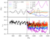 |
Fig. 19. Time evolution of the volume-averaged magnetic field component (⟨By⟩; first image) and the magnetic stress to pressure ratio (rsp = ⟨ − 2BxBy⟩/⟨|B|2⟩, second image). The time axis starts at tΩ0 = 600 and extends towards tΩ0 = 1600. Simulation sg-eta01 was run until 2400 |


In Sect. 6.2 it is demonstrated that the magnetic stress to pressure ratio, rsp = ⟨ − 2BxBy⟩/⟨|B|2⟩, significantly decreases in the new, resistive state. Hence, rsp is chosen as a second indicator for resistive runs, shown in the second image of Fig. 19. For comparison, MRI-typical values are in the range 0.3–0.4. The line rsp = 0.3 is highlighted in Fig. 19, as the horizontal, dashed line. Clearly, the ideal-MHD case yields MRI-typical values, as discussed previously. And almost all resistive simulations are also consistent with rsp ∼ 0.3, except the cases sg-eta01 and sg-eta005. This can also be seen from the time-averaged values ⟨rsp⟩t, provided in the last column of Table 4. This is consistent with the previously discussed time evolution of ⟨By⟩. From this, one might conclude that the qualitative transition, from the ideal-MHD regime to the resistive-GI dynamo, occurs for ⟨⟨Rm⟩⟩t ≲ 500, or η ≳ 0.005 in code units.
7.2. Testing whether resistive GI-MRI coexistence is resolved
As can be seen from the first image of Fig. 19, only the lowest resistivity simulation (sg-eta0006) and the two simulations with the largest resistivity values (sg-eta01 and sg-eta005) yield clearly interpretable states. Simulation sg-eta0006 clearly shows a prolongation of the periodic field reversals, whereas sg-eta01 and sg-eta005 evolve into the new resistive-GI dynamo state. All simulations in between, are not easily interpretable. For the latter, one can see field reversals, or at least the tendency towards field reversals, but they occur in a significantly less periodic pattern. One possible explanation is that the intermediate simulations tend towards GI-MRI coexistence, but their proximity to the transition from GI-MRI coexistence to the resistive-GI dynamo, may cause the more irregular field reversals. This is supported by the magnetic stress to pressure ratio, rsp. Alternatively, these states may be comparable to the ideal-MHD, strong-GI case, sg-mhd-tau10, where field-reversals are also more irregular and where MRI may be absent. However, it is also possible that resistivity in sg-eta-0006 is not properly resolved and one essentially recovers the ideal-MHD case. One possible way to resolve the uncertainty is to simulate a state with one of the lower resistivity values and with higher resolution. One should then be able to discern possible differences. For that reason, two additional simulations with the second lowest resistivity value, η = 0.00167, are presented. The latter are in the following referred to as gi-mri-res-1 and gi-mri-res-2. The difference between the two simulations is that gi-mri-res-2 uses roughly twice the resolution of gi-mri-res-1; the resolution of gi-mri-res-1 is equal to that used in sg-eta00167. Important parameters for the two simulations are provided in Table 6. In contrast to sg-eta00167, gi-mri-res-1 was not restarted from the GI-MRI coexistence in sg-mhd-2 but instead from the pure-GI simulation GI072 (see Löhnert & Peeters 2022), at tΩ0 = 120. A magnetic seed field of ZNF type was introduced such that one obtains ⟨β⟩xy = 107 at the mid-plane, and the resistivity of η = 0.00167 was enabled at that moment. We note that this is equivalent to the ideal-MHD simulation sg-mhd-2 (also restarted from GI072; see Löhnert & Peeters 2022), except that now resistivity was enabled directly at field seeding. This is meant to avoid possible biases from the fact that GI-MRI coexistence was already present in sg-mhd-2, when resistivity was introduced. The second simulation addresses the possibility of unresolved resistivity. Assuming that the effective grid resistivity is in the range ηeff = 2 × 10⁻⁴ − 2 × 10⁻³, for the lower resolution of 440 points per 20 H, than the chosen resistivity is at best an order of magnitude above the grid value, or in the worst case roughly equal to the grid value. Using the same estimate for the higher resolution of 800 points per 20 H, one obtains ηeff = 6 × 10⁻⁵ − 2 × 10⁻⁴, which is significantly smaller than η = 0.00167, in any case. By comparing gi-mri-res-1 and 2, one should be able to locate differences originating from insufficient resolution. We note that gi-mri-res-2 required significantly more computational resources, than the other simulations presented here. For that reason, we chose the vertical box size of 7 H, instead of the usual 8 H. But, as shown in Sect. 5.2, changing the vertical box size to 6 H did not change the simulation outcome of sg-mhd-tau20, and the latter yields essentially equal stress levels to sg-mhd-2. Additionally, it was possible to run the simulation with a slightly larger Courant number, of CFL = 0.5, without causing numerical instabilities. The field initialisation in gi-mri-res-2 is equal to that in gi-mri-res-1. We first set up a simulation with only GI and the same physical parameters (τcΩ0, Q0, γ, and η), as those, used in gi-mri-res-1, except with higher resolution. The simulation was initialised in a homogeneous, stratified state (stratification includes self-gravity), and small (1% of the background value) random perturbations in density and pressure were added. At first, the growth of axisymmetric GI modes is observed, which break up into turbulence after ∼40 . The pure-GI state is then prolonged until tΩ0 = 100. At that moment, similar to gi-mri-res-1, a ZNF field with ⟨β⟩xy = 107 was introduced, and resistivity with η = 0.00167 was enabled.
Important parameters and quantities for the resistive simulations gi-mri-res-1 and 2.
Similar to the first image of Fig. 19, one can analyse the time evolution of the volume-averaged, toroidal magnetic field component, ⟨By⟩, for both simulations gi-mri-res-1 and 2. This is shown in the first image of Fig. 20. Both simulations display field reversals, although the reversals seen in gi-mri-res-2 appear to be slightly less periodic than those in gi-mri-res-1. But it is possible that the latter is merely a statistical coincidence. The oscillation amplitudes (for ⟨By⟩) observed for the two simulations are in good agreement. We note that the field reversals seen in Fig. 20 are more pronounced than those in Fig. 19, despite sg-eta00167 having equal parameters. This may be indicative that the simulations, shown in Fig. 19 may indeed require more time to obtain a new, saturated state. Moreover, the mean time period for one field reversal is longer, compared to the ideal-MHD cases (see also the discussion about the butterfly diagram below). We also evaluated the magnetic stress-to-pressure ratio, rsp = ⟨ − 2BxBy⟩/⟨|B|2⟩, for simulations gi-mri-res-1 and 2. The corresponding time evolution of rsp is shown in the second image of Fig. 20. One first notices that the time evolutions for gi-mri-res-1 and 2 are in good agreement. Secondly, the values are in the range rsp ≳ 0.3, in agreement with the ideal-MHD cases and the pure-MRI simulation. Shown in Fig. 21, are zt diagrams of the horizontally averaged, toroidal magnetic field component, ⟨By⟩xy. These diagrams can be compared to the ideal cases, shown in Fig. 3. One notices that the field reversals of gi-mri-res-1 and 2 are not as coherent as those seen in sg-mhd-2 and sg-mhd-tau20. Interestingly, the seed fields in both gi-mri-res-1 and sg-mhd-2 were introduced into the same GI-turbulent state, yet the butterfly pattern, in the resistive case, is less pronounced than that in the ideal case. More precisely, the zt diagrams of gi-mri-res-1 and 2 are more reminiscent to the ideal case sg-mhd-tau10. And also here, one can see the tendency to field oscillations with a shorter time period, above and below the mid-plane. This es especially pronounced in the zt diagram of gi-mri-res-2. Hence, this resistive dynamo state has similarities with the strong-GI dynamo state, observed in the ideal-MHD regime. Interestingly, the GI activity in gi-mri-res-1 and 2 is equal to that of the weak-GI cases in the ideal regime. Thus, resistivity clearly has an influence.
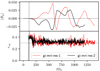 |
Fig. 20. Time evolution for both the volume-averaged magnetic field component, ⟨By⟩ (first image) and the magnetic stress-to-pressure ratio, rsp = ⟨ − 2BxBy⟩/⟨|B|2⟩ (second image). Simulation gi-mri-res-1 is depicted as the dashed red curve, and gi-mri-res-2 is shown as the black curve. For reference, the value rsp = 0.3 is shown as the horizontal dashed line in the second image. The vertical, dashed, and dotted lines mark the time points when the seed fields are introduced. |
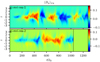 |
Fig. 21. zt diagrams of the horizontally averaged, toroidal magnetic field component, ⟨By⟩xy, for simulations gi-mri-res-1 and 2. |
The dimensionless, turbulent stresses are compared in Fig. 22, where the Reynolds, gravitational, and Maxwell contributions are shown from top to bottom. For gi-mri-res-2, the pure-GI phase (tΩ0 < 100) is depicted as well, and one can see a sharp spike (the spike was cut at the upper plot boundary), corresponding to the transition from the linear state to the nonlinear regime. Generally, the two simulations coincide well, which can also be read off from the time-averaged stresses, shown in Table 6. The absolute values of αm observed for gi-mri-res-1 and 2 are of the order of αm ∼ 0.006. This is slightly smaller than the pure MRI value (αm ∼ 0.0088) and smaller than the ideal-MHD runs with GI. Hence, it appears that Ohmic resistivity causes a reduction of αm. This is consistent with the observation that saturation of gi-mri-res-1 and 2 is similar to the strong-GI, ideal-MHD case, sg-mhd-tau10. Instead of GI being stronger, αm is here lower. Whether gi-mri-res-1 and 2 are states of GI-MRI coexistence is, similar to sg-mhd-tau10, not certain. A lower αm value, in the presence of resistivity, is at least not inconsistent with MRI. But the largest αm value, observed in this study, occurs for the most resistive simulation, sg-eta01 (αm ∼ 0.019; see Table 4). This implies that αm cannot decrease indefinitely, as η increases, and eventually some type of phase transition must occur. Taking into account the findings for the ideal-MHD cases, then this suggests that MRI fails at this point. But at the very least, some type of transition occurs. We note that this is consistent with the findings of Riols & Latter (2019), who also pointed out the possibility of a dynamo-state transition at Rm∼500 − 600.
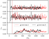 |
Fig. 22. Dimensionless turbulent stresses (Reynolds, gravitational, and Maxwell contributions, from top to bottom) as a function of time. The stresses for simulation gi-mri-res-1 are shown in dashed red, and the corresponding stresses for gi-mri-res-2 are shown as solid black curves. The vertical dashed and dotted lines correspond to the moments of field seeding for gi-mri-res-1 and 2, respectively. |
For reference, the mid-plane mass density, evaluated for gi-mri-res-2, at tΩ0 = 580, is shown in Fig. 23. The density plot is overlayed with a series of magnetic field lines, traced in the (x, y) plane, by only considering the field components (Bx, By). Similar to the previous cases, one observes a clearly visible alignment of the field lines with the density waves, related to GI. But similar to the ideal-MHD case, the field lines frequently change direction, in the regions between the density waves. Hence, small-scale structures are definitively present.
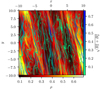 |
Fig. 23. Mid-plane mass density (z = 0) evaluated for gi-mri-res-2 at tΩ0 = 580. Superimposed are magnetic field lines traced in the (x, y) plane (only (Bx, By) were used for the tracing). |
One can conclude that doubling the resolution did not cause significant changes in the simulation outcome. And one can also see that a state with field reversals, and which has resemblance with the ideal-MHD states, can also be obtained from scratch, that is, without introducing resistivity into an already dynamo-saturated state. Hence, we conclude that the state, observed in Sect. 6, is indeed a new (third) dynamo state, and the observed transition, as Rm decreases, is indeed a physical effect originating from a significant heat production due to Ohmic resistivity.
8. Conclusion
Löhnert & Peeters (2022) report on the observation that the combined effects of self-gravity and magnetic fields can lead to a turbulent state that is consistent with a coexistence between GI and MRI. Here, this was further tested by varying the strength of GI, where strength refers to the pure-GI stress level (α, αg). The strength was controlled by varying the cooling law. Cases with τcΩ0 = 10 and additional heating were tested in Löhnert & Peeters (2022). Hence, additional simulations with cooling times τcΩ0 = 10 (strong-GI case) and 20 (weak-GI case) are provided here, and no additional heating was used. The strong-GI case (τcΩ0 = 10) leads to GI-only stresses that are larger by roughly a factor of two compared to the other simulations. At dynamo saturation, the weak-GI simulation leads to a clearly visible butterfly pattern, with sign reversals of ⟨By⟩xy, that is equivalent to those seen in Löhnert & Peeters (2022). That is different from the strong-GI case (τcΩ0 = 10). Clearly visible polarity reversals of ⟨By⟩xy are absent at the mid-plane, but one can see the tendency towards sign reversals above and below the mid-plane. The vertical EMF profiles, obtained for the weak-GI case (τcΩ0 = 20), are largely consistent with the EMFs derived from a pure-MRI reference simulation, though differences can be seen in the vertical field-strength distribution. For the strong-GI case (τcΩ0 = 10), differences to the pure-MRI simulation also arise in the vertical EMF profile. Hence, it appears that the weak-GI case (τcΩ0 = 20) and the strong-GI case (τcΩ0 = 10) lead to qualitatively different dynamo states. The τcΩ0 = 20 case has similarities to the pure-MRI simulation and is possibly a state of GI-MRI coexistence. The strong-GI case cannot be categorised exactly and is possibly a pure-GI dynamo. However, we note that the two states also share some similarities: the Maxwell stress, αm, is roughly equal in both the weak- and strong-GI cases, and the absolute reduction in the gravitational stress, αg (measured from the GI-only to the MHD-saturated state), is also equal. Hence, the absence (or presence) of MRI in the strong-GI case cannot definitively be settled in this context, though it appears that there are two different ideal-MHD dynamo states.
Löhnert & Peeters (2022) also report on differences to the simulations in Riols & Latter (2018a, 2019), especially the τcΩ0 = 20 case SGMRI-20 therein. They proposed that vertical outflows might be a possible source for discrepancies. For this purpose, an additional simulation with no heating, τcΩ0 = 20, and all remaining parameters equal to those in Riols & Latter (2018a) is presented here. This includes a slightly smaller box size, 6 H instead of our standard 8 H. The resulting turbulent state is equal to that of our standard runs, both qualitatively and quantitatively. We find that the discrepancies with Riols & Latter (2018a) arise from the difference in the duration (e.g. in units of  ) of the simulations, not the box size. For the first 320
 , after field seeding (duration of SGMRI-20) we find agreement. However, we find that, for the τcΩ0 = 20 case, saturation occurs ∼600
 after field seeding. At that point, a butterfly diagram that spans the entire vertical domain emerges. It is currently not clear why such a long saturation time is observed. One might speculate that it is related to vertical mixing due to GI. This may, at first, prevent field reversals near the mid-plane, though eventually the field strength can phase-lock the mid-plane field, inducing field reversals over the entire vertical domain. As a further test, we compared the τcΩ0 = 10 simulation to SGMRI-10 from Riols & Latter (2018a). The observed stresses for this cooling time are in agreement as well, though here we used the saturated phase for the average. We note that SGMRI-10 from Riols & Latter (2018a) was restarted from SGMRI-20, indicating that this case was closer to saturation.
We then tested how Ohmic resistivity influences GI-MRI coexistence. For that purpose, ideal-MHD simulations with fully developed turbulence and saturated dynamo were restarted with a finite value of Ohmic resistivity, η. The initial, ideal-MHD state can be characterised as a state of coexistence between gravitational turbulence and magneto-rotational turbulence, outlined in more detail in Löhnert & Peeters (2022). When the restart is undertaken with a resistivity, η, such that the magnetic Reynolds number is ⟨Rm⟩∼280 (η = 0.01 in code units), the system is at first disrupted but settles into a new nonlinear state after ∼300 . The new turbulent state is qualitatively different from the original state in the ideal-MHD regime. Most notably, the saturation level of the magnetic field strength doubles, reducing the plasma β by roughly a factor of four. The vertical geometry of the magnetic field also changes: the butterfly diagram, which is clearly visible in the ideal-MHD regime, is no longer visible with the introduction of resistivity. Additionally, the ratio of Maxwell stress to magnetic pressure in the resistive state is rsp ∼ 0.17, which is half the expected value for MRI (0.3 − 0.4). This shows that the newly developed state is qualitatively different from the ideal-MHD states and that MRI is effectively suppressed. The turbulent state develops oscillatory behaviour in time, but the origin of the oscillations is not an MRI-related butterfly diagram. Rather, it is the heat production due to Ohmic resistivity. As the GI dynamo builds up further magnetic energy, the Ohmic dissipation also increases, giving rise to enhanced heat production. The additional heat weakens the GI, which corresponds to a larger Toomre parameter value. This reduces dynamo activity, and the magnetic energy decays. Eventually, cooling reduces the thermal-energy level enough to reignite GI, and a new cycle begins. We refer to the new state as resistive-GI dynamo.
We then demonstrated that states consistent with the ideal-MHD regime can also occur when explicit resistivity is enabled. This was achieved in two steps. First, we derived an estimate for the effective grid resistivity, which we then used as a reference when scanning different resistivity values. The scan contains resistivity values in the range 6 × 10⁻⁴ ≤ η ≤ 0.01, which corresponds to magnetic Reynolds numbers of 280 ≲ ⟨⟨Rm⟩⟩t ≲ 4000. The transition appears to occur in the range Rm ∼ 470 − 680, although the value may be higher because the newly formed turbulent states could not easily be attributed to either GI-MRI coexistence or the resistive-GI dynamo. We argue that the best qualifier for this type of turbulence is the magnetic stress-to-pressure ratio, rsp = ⟨ − 2BxBy⟩/⟨|B|2⟩, which shows a clear transition in the range η ∼ 0.033 − 0.005 (⟨⟨Rm⟩⟩t ∼ 470 − 680). In a second step, we tested whether this transition is the artefact of an unresolved resistive dissipation scale or if it is due to the fact that the resistive simulations were restarted from an ideal-MHD state with GI-MRI coexistence. For this purpose, two additional simulations were provided; both simulations start with GI-only turbulence, and a small ZNF-type magnetic seed field was introduced. Both simulations used the same value of resistivity, η = 0.00167, or ⟨⟨Rm⟩⟩t ∼ 1400, which correspond to the second lowest value of the previous scan, but the second simulation used roughly twice the resolution of the first simulation. A turbulent state, consistent with the ideal-MHD regime, was obtained in both cases. This is implied by the magnetic stress-to-pressure ratio rsp ≳ 0.3 and the field reversals seen in the volume-averaged magnetic field component, ⟨By⟩. Furthermore, all quantitative measures that were tested are almost equal for the two simulations. Hence, we conclude that resolution does not change the simulation outcome and that states consistent with the ideal-MHD regime can also be found with explicit Ohmic resistivity. Whether MRI is present in these resistive cases is not entirely clear, as the saturated states are, in some aspects, akin to the ideal-MHD strong-GI case sg-mhd-tau10. The simulation outcomes do clearly suggest that some form of state transition must occur for Rm ∼500.
References
- Armitage, P. J. 2011, ARA&A, 49, 409 [Google Scholar]
- Armitage, P. J., Livio, M., & Pringle, J. E. 2001, MNRAS, 324, 705 [NASA ADS] [CrossRef] [Google Scholar]
- Bai, X.-N., & Stone, J. M. 2013, ApJ, 767, 30 [NASA ADS] [CrossRef] [Google Scholar]
- Balbus, S. A., & Hawley, J. F. 1991, ApJ, 376, 214 [Google Scholar]
- Balbus, S. A., & Hawley, J. F. 1998, Rev. Mod. Phys., 70, 1 [Google Scholar]
- Béthune, W., & Latter, H. 2022, A&A, 663, A138 [NASA ADS] [CrossRef] [EDP Sciences] [Google Scholar]
- Blackman, E. G., Penna, R. F., & Varnière, P. 2008, New Astron., 13, 244 [NASA ADS] [CrossRef] [Google Scholar]
- Boley, A. C., Mejía, A. C., Durisen, R. H., et al. 2006, ApJ, 651, 517 [Google Scholar]
- Booth, R. A., & Clarke, C. J. 2019, MNRAS, 483, 3718 [Google Scholar]
- Brandenburg, A., & Donner, K. J. 1997, MNRAS, 288, L29 [NASA ADS] [CrossRef] [Google Scholar]
- Brandenburg, A., Nordlund, A., Stein, R. F., & Torkelsson, U. 1995, ApJ, 446, 741 [NASA ADS] [CrossRef] [Google Scholar]
- Colella, P. 1990, J. Comput. Phys., 87, 171 [CrossRef] [MathSciNet] [Google Scholar]
- Colella, P., & Woodward, P. R. 1984, J. comput. Phys., 54, 174 [NASA ADS] [CrossRef] [Google Scholar]
- Coleman, M. S. B., Yerger, E., Blaes, O., Salvesen, G., & Hirose, S. 2017, MNRAS, 467, 2625 [NASA ADS] [CrossRef] [Google Scholar]
- Cossins, P., Lodato, G., & Clarke, C. J. 2009, MNRAS, 393, 1157 [Google Scholar]
- Courant, R., Friedrichs, K., & Lewy, H. 1928, Math. Ann., 100, 32 [Google Scholar]
- Davis, S. W., Stone, J. M., & Pessah, M. E. 2010, ApJ, 713, 52 [NASA ADS] [CrossRef] [Google Scholar]
- Deng, H., Mayer, L., & Latter, H. 2020, ApJ, 891, 154 [Google Scholar]
- Fromang, S. 2005, A&A, 441, 1 [NASA ADS] [CrossRef] [EDP Sciences] [Google Scholar]
- Fromang, S., Balbus, S. A., Terquem, C., & De Villiers, J.-P. 2004, ApJ, 616, 364 [NASA ADS] [CrossRef] [Google Scholar]
- Fromang, S., Papaloizou, J., Lesur, G., & Heinemann, T. 2007, A&A, 476, 1123 [NASA ADS] [CrossRef] [EDP Sciences] [Google Scholar]
- Fromang, S., Latter, H., Lesur, G., & Ogilvie, G. I. 2013, A&A, 552, A71 [NASA ADS] [CrossRef] [EDP Sciences] [Google Scholar]
- Gammie, C. F. 2001, ApJ, 553, 174 [Google Scholar]
- Goodman, J. 2003, MNRAS, 339, 937 [NASA ADS] [CrossRef] [Google Scholar]
- Gressel, O. 2010, MNRAS, 405, 41 [NASA ADS] [CrossRef] [Google Scholar]
- Guan, X., & Gammie, C. F. 2011, ApJ, 728, 130 [NASA ADS] [CrossRef] [Google Scholar]
- Hawley, J. F., & Balbus, S. A. 1992, ApJ, 400, 595 [NASA ADS] [CrossRef] [Google Scholar]
- Hawley, J. F., Gammie, C. F., & Balbus, S. A. 1995, ApJ, 440, 742 [Google Scholar]
- Hawley, J. F., Guan, X., & Krolik, J. H. 2011, ApJ, 738, 84 [NASA ADS] [CrossRef] [Google Scholar]
- Hirose, S., & Shi, J.-M. 2019, MNRAS, 485, 266 [Google Scholar]
- Hirose, S., Blaes, O., Krolik, J. H., Coleman, M. S. B., & Sano, T. 2014, ApJ, 787, 1 [NASA ADS] [CrossRef] [Google Scholar]
- Käpylä, P. J., & Korpi, M. J. 2011, MNRAS, 413, 901 [CrossRef] [Google Scholar]
- Koyama, H., & Ostriker, E. C. 2009, ApJ, 693, 1316 [NASA ADS] [CrossRef] [Google Scholar]
- Kratter, K., & Lodato, G. 2016, ARA&A, 54, 271 [NASA ADS] [CrossRef] [Google Scholar]
- Lesur, G., & Ogilvie, G. I. 2008, A&A, 488, 451 [NASA ADS] [CrossRef] [EDP Sciences] [Google Scholar]
- Lin, C. C., & Shu, F. H. 1964, ApJ, 140, 646 [Google Scholar]
- Lin, M.-K., & Kratter, K. M. 2016, ApJ, 824, 91 [Google Scholar]
- Lodato, G., & Rice, W. K. M. 2004, MNRAS, 351, 630 [Google Scholar]
- Löhnert, L., & Peeters, A. G. 2022, A&A, 663, A176 [NASA ADS] [CrossRef] [EDP Sciences] [Google Scholar]
- Lynden-Bell, D. 1969, Nature, 223, 690 [NASA ADS] [CrossRef] [Google Scholar]
- Lynden-Bell, D., & Kalnajs, A. J. 1972, MNRAS, 157, 1 [Google Scholar]
- Martin, R. G., & Lubow, S. H. 2011, ApJ, 740, L6 [NASA ADS] [CrossRef] [Google Scholar]
- Martin, R. G., Lubow, S. H., Livio, M., & Pringle, J. E. 2012, MNRAS, 423, 2718 [NASA ADS] [CrossRef] [Google Scholar]
- Masset, F. 2000, A&AS, 141, 165 [NASA ADS] [CrossRef] [EDP Sciences] [Google Scholar]
- Menou, K., & Quataert, E. 2001, ApJ, 552, 204 [NASA ADS] [CrossRef] [Google Scholar]
- Oishi, J. S., & Mac Low, M.-M. 2011, ApJ, 740, 18 [NASA ADS] [CrossRef] [Google Scholar]
- Paardekooper, S.-J. 2012, MNRAS, 421, 3286 [Google Scholar]
- Rice, W. K. M., Armitage, P. J., Bate, M. R., & Bonnell, I. A. 2003, MNRAS, 339, 1025 [Google Scholar]
- Rice, W. K. M., Armitage, P. J., Mamatsashvili, G. R., Lodato, G., & Clarke, C. J. 2011, MNRAS, 418, 1356 [Google Scholar]
- Riols, A., & Latter, H. 2018a, MNRAS, 474, 2212 [NASA ADS] [CrossRef] [Google Scholar]
- Riols, A., & Latter, H. 2018b, MNRAS, 476, 5115 [Google Scholar]
- Riols, A., & Latter, H. 2019, MNRAS, 482, 3989 [Google Scholar]
- Riols, A., Latter, H., & Paardekooper, S.-J. 2017, MNRAS, 471, 317 [Google Scholar]
- Riols, A., Xu, W., Lesur, G., Kunz, M. W., & Latter, H. 2021, MNRAS, 506, 1407 [NASA ADS] [CrossRef] [Google Scholar]
- Roe, P. L. 1981, J. Comput. Phys., 43, 357 [Google Scholar]
- Rüdiger, G., & Pipin, V. V. 2000, A&A, 362, 756 [NASA ADS] [Google Scholar]
- Salvesen, G., Simon, J. B., Armitage, P. J., & Begelman, M. C. 2016, MNRAS, 457, 857 [Google Scholar]
- Sanders, R., Morano, E., & Druguet, M.-C. 1998, J. Comput. Phys., 145, 511 [NASA ADS] [CrossRef] [Google Scholar]
- Sano, T., & Stone, J. M. 2002, ApJ, 577, 534 [NASA ADS] [CrossRef] [Google Scholar]
- Sano, T., Inutsuka, S.-I., & Miyama, S. M. 1998, ApJ, 506, L57 [NASA ADS] [CrossRef] [Google Scholar]
- Shakura, N. I., & Sunyaev, R. A. 1973, A&A, 24, 337 [NASA ADS] [Google Scholar]
- Shi, J.-M., & Chiang, E. 2014, ApJ, 789, 34 [Google Scholar]
- Shi, J., Krolik, J. H., & Hirose, S. 2009, ApJ, 708, 1716 [Google Scholar]
- Silvers, L. J. 2008, MNRAS, 385, 1036 [NASA ADS] [CrossRef] [Google Scholar]
- Simon, J. B., & Hawley, J. F. 2009, ApJ, 707, 833 [NASA ADS] [CrossRef] [Google Scholar]
- Simon, J. B., Hawley, J. F., & Beckwith, K. 2011, ApJ, 730, 94 [NASA ADS] [CrossRef] [Google Scholar]
- Stone, J. M., & Gardiner, T. A. 2010, ApJS, 189, 142 [NASA ADS] [CrossRef] [Google Scholar]
- Stone, J. M., Hawley, J. F., Gammie, C. F., & Balbus, S. A. 1996, ApJ, 463, 656 [NASA ADS] [CrossRef] [Google Scholar]
- Stone, J. M., Gardiner, T. A., Teuben, P., Hawley, J. F., & Simon, J. B. 2008, ApJS, 178, 137 [NASA ADS] [CrossRef] [Google Scholar]
- Suzuki, T. K., & Inutsuka, S.-I. 2009, ApJ, 691, L49 [Google Scholar]
- Toomre, A. 1964, ApJ, 139, 1217 [Google Scholar]
- Turner, N. J., Sano, T., & Dziourkevitch, N. 2007, ApJ, 659, 729 [NASA ADS] [CrossRef] [Google Scholar]
- Young, M. D., & Clarke, C. J. 2015, MNRAS, 451, 3987 [Google Scholar]
- Zhu, Z., Hartmann, L., & Gammie, C. 2009, ApJ, 694, 1045 [Google Scholar]
- Zhu, Z., Hartmann, L., & Gammie, C. 2010, ApJ, 713, 1143 [Google Scholar]
- Ziegler, U., & Rüdiger, G. 2000, A&A, 356, 1141 [NASA ADS] [Google Scholar]
- Ziegler, U., & Rüdiger, G. 2001, A&A, 378, 668 [NASA ADS] [CrossRef] [EDP Sciences] [Google Scholar]
- Zier, O., & Springel, V. 2023, MNRAS, 520, 3097 [NASA ADS] [CrossRef] [Google Scholar]
Appendix A: Prolongation of sg-mhd-tau10
In Sect. 5.1, a direct comparison between the pure-GI phase and the dynamo-saturated phase of simulation sg-mhd-tau10 is provided. The pure-GI phase (B = 0), of simulation sg-mhd-tau10, exhibits significant oscillations in αr and αg. This is not the case in the dynamo-saturated phase. Hence, in order to obtain more reliable statistics, the pure-GI phase, of sg-mhd-tau10, was prolonged, from tΩ0 = 400 to 700. The corresponding stresses and the Toomre parameter are shown in Fig. A.1. At tΩ0 = 200 (vertical, dashed line), sg-mhd-tau10 was restarted from sg-mhd-tau20, but with a lower cooling time of τcΩ0 = 10. In the original simulation, the ZNF-seed field is introduced at tΩ0 = 400. Here, the pure-GI phase (B = 0) is prolonged, instead. The average is then taken over the 500 − 700 interval, highlighted by the black, vertical lines. The resulting, time-averaged values are shown in Table 2.
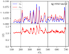 |
Fig. A.1. Prolonged, pure-GI phase of simulation sg-mhd-tau10. At tΩ0 = 200 (vertical dashed line), sg-mhd-tau10 was restarted from the pure-GI phase of sg-mhd-tau20. The boundaries of the interval used for the time average are depicted as the vertical black lines. |
All Tables
Comparison of the initial and saturated phases for simulations sg-mhd-tau20 and 10.
Important parameters and quantities for the resistive simulations gi-mri-res-1 and 2.
All Figures
|
Fig. 1. Volume-averaged Toomre parameter, ⟨Q⟩, evaluated for simulations sg-mhd-tau10 (red) and sg-mhd-tau20 (blue). The vertical lines indicate the times at which the seed fields were introduced. |
| In the text | |
|
Fig. 2. Dimensionless stresses as a function of time for simulations sg-mhd-tau20 (τcΩ0 = 20), sg-mhd-tau10 (τcΩ0 = 10), sg-mhd-2 (τcΩ0 = 10, Q0 ∼ 0.75), and MRI-compare. Shown in blue is the Reynolds contribution, αr, in red the gravitational contribution, αg, and in black the Maxwell part, αm. All stresses were calculated using Eqs. (8) and (9), and the factor γ = 1.64 was also used for the isothermal MRI, allowing for an easier comparison. The curves for sg-mhd-tau20 and 10 start at tΩ0 = 120, at which point the simulations were restarted from the pure-GI state of GI072 (see Löhnert & Peeters 2022). Then, the cooling time was set to τcΩ0 = 20, and background heating was turned off (only cooling). At tΩ0 = 200, either one of two things happens, depending on the simulation. In sg-mhd-tau20, the ZNF field was introduced directly at tΩ0 = 200, highlighted by the solid vertical line. In sg-mhd-tau10, the pure-GI phase was prolonged from tΩ0 = 200 (vertical dashed line) to tΩ0 = 400 (vertical solid line), but the cooling time was reduced to τcΩ0 = 10. At tΩ0 = 400, the ZNF field was introduced. For both sg-mhd-tau20 and 10, the values of αg and αr were smoothed by convolving the respective time series with a Gaussian function (standard deviation σ = 3 |
| In the text | |
|
Fig. 3. Horizontally averaged toroidal magnetic field component, ⟨By⟩xy, as a function height, z, and time, t. The zt diagrams are shown for simulations sg-mhd-2, sg-mhd-tau20, sg-mhd-tau10, and MRI-compare. The time axis is chosen such that t = 0 corresponds to the moment of field seeding. |
| In the text | |
|
Fig. 4. Sign of the horizontally averaged toroidal magnetic field component. In this case, the “sign” has been intended to be a mathematical function, returning the sign of a value. sign(⟨By⟩xy), shown for simulations sg-mhd-tau10 and sg-mhd-tau20. The images can be directly compared to the corresponding zt diagrams in Fig. 3. |
| In the text | |
|
Fig. 5. Inverse volume-averaged plasma β, ⟨β⟩−1 = ⟨|B|2⟩/(2μ0⟨P⟩), and the ratio of Maxwell stress to magnetic pressure, rsp = ⟨ − 2BxBy⟩/(|B|2), as a function of time. The depicted simulations are sg-mhd-tau10 (red), sg-mhd-tau20 (blue), sg-mhd-2 (black), and MRI-compare (cyan). In all cases, the time t = 0 corresponds to the moment of field seeding. |
| In the text | |
|
Fig. 6. Mid-plane mass density, ρ(x, y, z = 0), for simulation sg-mhd-tau20 evaluated at tΩ0 = 1200. The mass density is superimposed with magnetic field lines traced in the (x, y) plane with only the Bx and By components used for the tracing. |
| In the text | |
|
Fig. 7. Time evolution for a selection of quantities evaluated for sg-mhd-tau20-Lz6. First image: Dimensionless stresses as a function of time. Shown in blue is the Reynolds contribution, αr, in red the gravitational contribution, αg, and in black the Maxwell part, αm. All stresses were calculated, using Eqs. (8) and (9). The values of αr, and αg were smoothed using a Gaussian function (see also Fig. 2). Second image: Horizontally averaged magnetic field component, ⟨By⟩xy, as a function of height, z, and time, t. At tΩ0 = 200 (vertical solid line), the magnetic seed field is introduced. The vertical dashed line corresponds to 320 |
| In the text | |
|
Fig. 8. Horizontally averaged field components and EMFs as a function of z. Solid curves correspond to sg-mhd-tau20, and dashed curves correspond to MRI-compare. The first two images depict ℰx, and ℰy, respectively. Images three and four show the magnetic field components Bx and By, respectively. The red curves were averaged over the 200 − 400 |
| In the text | |
|
Fig. 9. Horizontally averaged field components and EMFs as a function of z, equivalent to Fig. 8 except now evaluated for simulation sg-mhd-tau10. Red curves are averages over the 400 − 600 |
| In the text | |
|
Fig. 10. Magnetic energy fluxes as a function of time evaluated for both sg-mhd-tau20 (black curves) and MRI-compare (red curves). Shown in the first image is the conversion rate from magnetic to kinetic energy, ⟨(v × B)⋅J⟩. This rate was calculated using the central differences from the full three-dimensional output data every 10 |
| In the text | |
|
Fig. 11. Absolute values of the field line bending forces, ⟨⟨|(B ⋅ ∇)Bx, y|⟩xy⟩t (solid curves), and the self-gravity forces, ⟨⟨|ρ∂x, yΦ|⟩xy⟩t (dashed curves), in directions x (red) and y (blue), evaluated for simulation sg-mhd-tau20. The time average is over the interval 800 ≤ tΩ0 ≤ 1300. The force densities were calculated using finite differences from the full three-dimensional output data of Athena every 10 |
| In the text | |
|
Fig. 12. Time evolutions for a selection of volume-averaged quantities evaluated for sg-eta01. First image: Turbulent stresses αr (Reynolds), αm (Maxwell), and αg (gravitational) as a function of time. The values for both αg and αr were smoothed by convolving the respective time series with a Gaussian function and with a standard deviation of σ = 3 |
| In the text | |
|
Fig. 13. Vertical profile of the normalised, horizontally averaged magnetic field component, |
| In the text | |
|
Fig. 14. Mass density at z = 0 and tΩ0 = 2000 for simulation sg-eta01. The image is overlayed with magnetic field lines traced in the (x, y) plane and only using the field components (Bx, By). |
| In the text | |
|
Fig. 15. Time evolution of the volume-averaged Toomre parameter, ⟨Q⟩ (red curve), and the dimensionless gravitational stress, αg (black curve), evaluated for sg-eta01. The vertical dashed line at tΩ0 = 1000 marks the time point at which resistivity is introduced. The αg values were smoothed using a Gaussian function with standard deviation σ = 3 |
| In the text | |
|
Fig. 16. Negative cooling (heating) rate ( |
| In the text | |
|
Fig. 17. Contributions to the magnetic energy balance evaluated for sg-eta01 as a function of time. All values are normalised by the momentary magnetic energy density, Emag. Shown in blue is the volume-averaged rate at which magnetic energy is converted to kinetic energy, ⟨v × B ⋅ J⟩. The values were calculated from the full three-dimensional output data using central differences every 10 |
| In the text | |
|
Fig. 18. Volume-averaged magnetic energy density, Emag, for the ideal-MHD simulations sg-mhd-2 (black), sg-mhd-tau10 (red), and sg-mhd-tau20 (blue) and the resistive simulation sg-eta01 (cyan). The time axis starts at t = 0 for all simulations. For the ideal-MHD runs, this corresponds to the moment of field seeding and for the resistive run, (t = 0) corresponds to the moment when resistivity was introduced. The dashed black lines correspond to linear fits, according to the values in Table 5. |
| In the text | |
|
Fig. 19. Time evolution of the volume-averaged magnetic field component (⟨By⟩; first image) and the magnetic stress to pressure ratio (rsp = ⟨ − 2BxBy⟩/⟨|B|2⟩, second image). The time axis starts at tΩ0 = 600 and extends towards tΩ0 = 1600. Simulation sg-eta01 was run until 2400 |
| In the text | |
|
Fig. 20. Time evolution for both the volume-averaged magnetic field component, ⟨By⟩ (first image) and the magnetic stress-to-pressure ratio, rsp = ⟨ − 2BxBy⟩/⟨|B|2⟩ (second image). Simulation gi-mri-res-1 is depicted as the dashed red curve, and gi-mri-res-2 is shown as the black curve. For reference, the value rsp = 0.3 is shown as the horizontal dashed line in the second image. The vertical, dashed, and dotted lines mark the time points when the seed fields are introduced. |
| In the text | |
|
Fig. 21. zt diagrams of the horizontally averaged, toroidal magnetic field component, ⟨By⟩xy, for simulations gi-mri-res-1 and 2. |
| In the text | |
|
Fig. 22. Dimensionless turbulent stresses (Reynolds, gravitational, and Maxwell contributions, from top to bottom) as a function of time. The stresses for simulation gi-mri-res-1 are shown in dashed red, and the corresponding stresses for gi-mri-res-2 are shown as solid black curves. The vertical dashed and dotted lines correspond to the moments of field seeding for gi-mri-res-1 and 2, respectively. |
| In the text | |
|
Fig. 23. Mid-plane mass density (z = 0) evaluated for gi-mri-res-2 at tΩ0 = 580. Superimposed are magnetic field lines traced in the (x, y) plane (only (Bx, By) were used for the tracing). |
| In the text | |
|
Fig. A.1. Prolonged, pure-GI phase of simulation sg-mhd-tau10. At tΩ0 = 200 (vertical dashed line), sg-mhd-tau10 was restarted from the pure-GI phase of sg-mhd-tau20. The boundaries of the interval used for the time average are depicted as the vertical black lines. |
| In the text | |
Current usage metrics show cumulative count of Article Views (full-text article views including HTML views, PDF and ePub downloads, according to the available data) and Abstracts Views on Vision4Press platform.
Data correspond to usage on the plateform after 2015. The current usage metrics is available 48-96 hours after online publication and is updated daily on week days.
Initial download of the metrics may take a while.