| Issue |
A&A
Volume 672, April 2023
|
|
|---|---|---|
| Article Number | A122 | |
| Number of page(s) | 30 | |
| Section | Interstellar and circumstellar matter | |
| DOI | https://doi.org/10.1051/0004-6361/202245097 | |
| Published online | 12 April 2023 | |
ALMA ACA study of the H2S/OCS ratio in low-mass protostars
1
Université Bourgogne Franche-Comté,
32 Avenue de l’Observatoire,
25000
Besançon, France
e-mail: This email address is being protected from spambots. You need JavaScript enabled to view it.
2
School of Physics and Astronomy, Cardiff University,
The Parade,
Cardiff
CF24 3AA, UK
e-mail: This email address is being protected from spambots. You need JavaScript enabled to view it.
3
Center for Space and Habitability, Universität Bern,
Gesellschaftsstrasse 6,
3012
Bern, Switzerland
e-mail: This email address is being protected from spambots. You need JavaScript enabled to view it.
4
European Southern Observatory,
Karl-Schwarzschild-Strasse 2,
85748
Garching bei München, Germany
5
Université Paris-Saclay, CNRS, Institut d’Astrophysique Spatiale,
91405
Orsay, France
Received:
29
September
2022
Accepted:
14
February
2023
Abstract
Context. The identification of the main sulfur reservoir on its way from the diffuse interstellar medium to the cold dense star-forming cores and, ultimately, to protostars is a long-standing problem. Despite sulfur’s astrochemical relevance, the abundance of S-bearing molecules in dense cores and regions around protostars is still insufficiently constrained.
Aims. The goal of this investigation is to derive the gas-phase H2S/OCS ratio for several low-mass protostars, which could provide crucial information about the physical and chemical conditions in the birth cloud of Sun-like stars. This may also shed new light onto the main sulfur reservoir in low-mass star-forming systems.
Methods. Using Atacama Large Millimeter/submillimeter Array (ALMA) Atacama Compact Array (ACA) Band 6 observations, we searched for H2S, OCS, and their isotopologs in ten Class 0/I protostars with different source properties such as age, mass, and environmental conditions. The sample contains IRAS 16293-2422 A, IRAS 16293-2422 B, NGC 1333-IRAS 4A, RCrA IRS7B, Per-B1-c, BHR71-IRS1, Per-emb-25, NGC 1333-IRAS4B, Ser-SMM3, and TMC1. A local thermal equilibrium (LTE) model is used to fit synthetic spectra to the detected lines and to derive the column densities based solely on optically thin lines.
Results. The H2S and OCS column densities span four orders of magnitude across the sample. The H2S/OCS ratio is found to be in the range from 0.2 to above 9.7. IRAS 16293-2422 A and Ser-SMM3 have the lowest ratio, while BHR71-IRS1 has the highest. Only the H2S/OCS ratio of BHR71-IRS1 is in agreement with the ratio in comet 67P/Churyumov–Gerasimenko within the uncertainties.
Conclusions. The determined gas-phase H2S/OCS ratios can be below the upper limits on the solid-state ratios by as much as one order of magnitude. The H2S/OCS ratio depends in great measure on the environment of the birth cloud, such as UV-irradiation and heating received prior to the formation of a protostar. The highly isolated birth environment (a Bok globule) of BHR71-IRS1 is hypothesized as the reason for its high gaseous H2S/OCS ratio that is due to lower rates of photoreactions and more efficient hydrogenation reactions under such dark, cold conditions. The gaseous inventory of S-bearing molecules in BHR71-IRS1 appears to be the most similar to that of interstellar ices.
Key words: astrochemistry / line: identification / instrumentation: interferometers / ISM: molecules / stars: protostars
© The Authors 2023
 Open Access article, published by EDP Sciences, under the terms of the Creative Commons Attribution License (https://creativecommons.org/licenses/by/4.0), which permits unrestricted use, distribution, and reproduction in any medium, provided the original work is properly cited.
This article is published in open access under the Subscribe to Open model. This email address is being protected from spambots. You need JavaScript enabled to view it. to support open access publication.
1 Introduction
Sulfur (S) is the tenth most abundant element in the Universe (S/H~1.35×10−5, Yamamoto 2017). It was first detected as carbon monosulfide (CS) in the interstellar medium (Penzias et al. 1971). Since then, S-bearing species have been detected in different regions including molecular clouds (Navarro-Almaida et al. 2020; Spezzano et al. 2022), hot cores (Blake et al. 1987; Charnley 1997; Li et al. 2015; Codella et al. 2021; Drozdovskaya et al. 2018), comets (Smith et al. 1980; Bockelée-Morvan et al. 2000; Biver et al. 2021a,b), and starburst galaxies (NGC 253; Martín et al. 2005). The total abundance of an element in dust, ice, and gas is its cosmic abundance, also called its elemental abundance. The gas-phase abundance of atomic sulfur in diffuse clouds is comparable to the cosmic abundance of sulfur (~10−5; Savage & Sembach 1996; Howk et al. 2006). However, the observed abundance of S-bearing species in dense cores and protostellar environments is lower by a factor of ~ 1000 (Snow et al. 1986; Tieftrunk et al. 1994; Goicoechea et al. 2006; Agúndez et al. 2018) in comparison to the total S-abundance in diffuse clouds. The forms and mechanisms behind this sulfur depletion in star-forming regions are still unknown. This is often referred to as the “missing sulfur problem.”
Different chemical models have been used to investigate this unknown form of sulfur (Woods et al. 2015; Vidal et al. 2017; Semenov et al. 2018; Vidal & Wakelam 2018; Laas & Caselli 2019). Vidal et al. (2017) proposed that a notable amount of sulfur is locked up in either HS and H2S ices or gaseous atomic sulfur in cores, depending in large part on the age of the molecular cloud. However, the only solid form of sulfur firmly detected in interstellar ices is OCS (Palumbo et al. 1995, 1997; Aikawa et al. 2012; Boogert et al. 2015) as well as potentially SO2 (Boogert et al. 1997; Zasowski et al. 2009; Yang et al. 2022; McClure et al. 2023). At the same time, solid-state H2S detection remains tentative to date (Geballe et al. 1985; Smith 1991). The initial cloud abundance of S-bearing molecules has been shown to set the subsequent abundances of these molecules in protostellar regions, depending on the free-fall timescales (Vidal & Wakelam 2018). In surface layers of protoplanetary disks, the availability of gaseous S-bearing molecules appears to be strongly linked with the availability of oxygen (Semenov et al. 2018). Observational studies of gas-phase species claim either H2S (Holdship et al. 2016) or OCS (van der Tak et al. 2003) as the main S-carrier depending on the environment being observed. Other possible reservoirs of sulfur have been proposed in the form of semi-refractory polymers up to S8 (A’Hearn et al. 1983; Druard & Wakelam 2012; Calmonte et al. 2016; Shingledecker et al. 2020), hydrated sulfuric acid (Scappini et al. 2003), atomic sulfur (Anderson et al. 2013), and mineral sulfides, FeS (Keller et al. 2002; Köhler et al. 2014; Kama et al. 2019). On the other hand, chemical models of the evolution from cloud to dense core with updated chemical networks suggest that sulfur is merely partitioned over a diverse set of simple organo-sulfur ices and no additional form is required (Laas & Caselli 2019). Matching observed and modeled cloud abundances consistently for the full inventory of gaseous S-bearing molecules to better than a factor of 10 remains challenging (Navarro-Almaida et al. 2020). Laboratory experiments point to the importance of the photodissociation of H2S ice by UV photons leading to the production of OCS ice (Ferrante et al. 2008; Garozzo et al. 2010; Jiménez-Escobar & Muñoz Caro 2011; Chen et al. 2015) and S2 in mixed ices (Grim & Greenberg 1987). Calmonte et al. (2016) claim to have recovered the full sulfur inventory in comets.
Sulfur-bearing species have been proposed to probe the physical and chemical properties of star-forming regions and to even act as chemical clocks (Charnley 1997; Hatchell et al. 1998; Viti et al. 2001; Li et al. 2015). However, it has since been shown that their abundance is sensitive to the gas-phase chemistry and the availability of atomic oxygen, which puts their reliability as chemical clocks into question (Wakelam et al. 2004, 2011). Studying S-bearing molecules in young Class 0/I protostars is crucial for two reasons. Firstly, their inner hot regions thermally desorb all the volatile ices that are otherwise hidden from gasphase observations. Consequently, it is more likely to be able to probe the full volatile inventory of S-bearing molecules and investigate the “missing sulfur” reservoir. Secondly, these targets are a window onto the materials available for the assembly of the protoplanetary disk midplane and the cometesimals therein (Aikawa & Herbst 1999; Willacy 2007; Willacy & Woods 2009). This makes hot inner regions highly suitable targets for comparative studies with comets (Bockelée-Morvan et al. 2000; Drozdovskaya et al. 2019).
The main goal of this paper is to study the physical and chemical conditions in embedded protostars via the H2S/OCS ratio. A sample of ten Class 0/I low-mass protostars with different physical properties (mass, age, and environment) is considered. Such protostars are in their earliest phase of formation after collapse with large envelope masses. In this work, Atacama Large Millimeter/submillimeter Array (ALMA) Atacama Compact Array (ACA) Band 6 observations towards these 10 protostars are utilized. The H2S/OCS ratio is calculated from the column densities of H2S, OCS, and their isotopologs. The details of the observations, model, and model parameters used for synthetic spectral fitting are introduced in Sect. 2. The detected lines of major and minor isotopologs of H2S and OCS, their characteristics, and H2S/OCS line ratios are presented in Sect. 3. The discussion and conclusions are presented in Sects. 4 and 5, respectively.
2 Methods
2.1 Observations
Two sets of observations are jointly analyzed in this paper. The first data set (project-id: 2017.1.00108.S; PI: M. N. Drozdovskaya) targets IRAS 16293-2422, NGC 1333-IRAS4A, and RCrA IRS7B. The relevant observations were carried out in Band 6 (211–275 GHz) with the ALMA ACA of 7 m dishes. The data set has a spectral resolution of 0.079–0.085 km s−1 (61 kHz), and a spatial resolution of (6.5–9.0)×(4.0–6.3)”. The second data set (project-id: 2017.1.1350.S; PI: Ł. Tychoniec) targets Per-B1-c, BHR71, Per-emb-25, NGC 1333-IRAS4B, Ser-SMM3, and TMC1 with the ALMA ACA 7m dishes, also in Band 6. The data have a similar spatial resolution, (6.1–7.4)×(4.5–6.4)″, but a lower spectral resolution of 0.333–0.678 km s−1 (244–488 kHz). The observed frequency ranges of the data are given in Table 1. The data cubes were processed through the standard pipeline calibration with CASA 5.4.0–68. For each source, the noise level has been calculated by taking the standard deviation of the flux in the frequency ranges where no emission lines were detected, that is, regions with pure noise in the spectral window containing the H2S, 22,0−21,1 line. The noise level of the first data set is between 21 and 32 mJy beam−1 channel−1 and that of the second data set is between 7 and 13 mJy beam−1 channel−1 (Table 3). Both data sets have a flux uncertainty of 10%. The largest resolvable scale of the first and the second data sets are 26.2–29.2″ and 24.6–29.0″, respectively.
2.2 Sources
The properties of the sources explored in this work are tabulated in Table 2. IRAS 16293-2422 (hereafter, IRAS 16293) is a triple protostellar source, consisting of protostars A and B, separated by 5.3″ (747 au; van der Wiel et al. 2019), and disk-like structures around the two sources, located in the Rho Ophiuchi star-forming region at a distance of 141 pc (Dzib et al. 2018). This source was studied thoroughly using ALMA under the Protostellar Interferometric Line Survey (PILS; Jørgensen et al. 2016) and many preceding observational campaigns (e.g., van Dishoeck et al. 1995; Caux et al. 2011). Both hot corinos around A and B are rich in a diverse set of complex organic molecules (Jørgensen et al. 2018; Manigand et al. 2020). The source IRAS 16293 A is itself a binary composed of sources A1 and A2 with a separation of 0.38″ (54 au; Maureira et al. 2020). IRAS4A is also a binary, made up of IRAS4A1 and IRAS4A2, separated by 1.8″ (540 au; Sahu et al. 2019) in the Perseus molecular cloud, located at a distance of 299 pc (Zucker et al. 2018) in the south-eastern edge of the complex NGC 1333 (Looney et al. 2000). IRAS4A1 has a much higher dust density in its envelope than IRAS4A2, but both contain complex organic molecules (Sahu et al. 2019; De Simone et al. 2020). IRS7B is a low-mass source, with a separation of 14″ (2 000 au) from IRS7A (Brown 1987), and ~8″ (1000 au) from CXO 34 (Lindberg et al. 2014). It is situated in the Corona Australis dark cloud at a distance of 130 pc (Neuhäuser & Forbrich 2008). IRS7B has been shown to contain lower complex organic abundances as a result of being located in a strongly irradiated environment (Lindberg et al. 2015).
From the second set of sources, IRAS4B (sometimes labeled BI) has a binary component B′ (or BII) that is 11″ (3300 au) away (Sakai et al. 2012; Anderl et al. 2016; Tobin et al. 2016). The separation between IRAS4B and IRAS4A is 31″ (9300 au; Coutens et al. 2013). IRAS4B displays emission from complex organic molecules (Belloche et al. 2020) and powers a highvelocity SiO jet (Podio et al. 2021). B1-c is an isolated deeply embedded protostar in the Barnard 1 clump in the western part of the Perseus molecular cloud at a distance of 301 pc (Zucker et al. 2018). B1-c contains emission from complex organic molecules and shows a high velocity outflow (Jørgensen et al. 2006; van Gelder et al. 2020). The next closest source, B1-a, is ~100″ (~29 500 ȧu) away (Jørgensen et al. 2006). BHR71 is a Bok globule in the Southern Coalsack dark nebulae at a distance of ~200 pc (Seidensticker & Schmidt-Kaler 1989; Straizys et al. 1994). It hosts the wide binary system of IRS1 and IRS2 with a sepration of 16″ (3200 au; Bourke 2001; Parise et al. 2006; Chen et al. 2008; Tobin et al. 2019). IRS1 displays pronounced emission from complex organic molecules (Yang et al. 2020). Emb-25 is a single source located in the Perseus molecularcloud (Enoch et al. 2009; Tobin et al. 2016). It does not show emission from complex organic molecules (Yang et al. 2021), but powers low-velocity CO outflows (Stephens et al. 2019). TMC1 is a Class I binary source, located in the Taurus molecular cloud (Chen et al. 1995; Brown & Chandler 1999) at a distance of 140 pc (Elias 1978; Torres et al. 2009). The separation between the two components, TMC1E and TMC1W, is ~0.6″ (~85 au); and neither of the two display complex organic emission (van’t Hoff et al. 2020). SMM3 is a single, embedded protostar located in the SE region in Serpens region; 436 pc away (Ortiz-León et al. 2018). The next closest-lying source is SMM6 at a separation of 20″ (~8700 au; Davis et al. 1999; Kristensen et al. 2010; Mirocha et al. 2021). SMM3 launches a powerful jet (Tychoniec et al. 2021), but does not display complex organic molecule emission, which may be obscured by the enveloping dust (van Gelder et al. 2020).
Spectral settings of the data sets.
Observed Class 0/I protostellar systems.
Location of the center position (in RA and Dec) and radius (in au and arcsecond) of each circular region, from which the spectra are extracted for the studied protostars.
2.3 Synthetic spectral fitting
For the spectral analysis, on-source spectra were extracted from the data cubes of the sources of the two data sets. Circular regions centered on source positions (in RA and Dec) with the radius of spectrum extraction corresponding to one-beam on-source are given in Table 3. The number of pixels in radius r of the circular region to be used was computed by dividing the radius of the circular region with the size of one pixel in arc-second. The spectroscopy used for the targeted molecules and their isotopologs stems from the Cologne Database of Molecular Spectroscopy (CDMS; Müller et al. 2001, 2005; Endres et al. 2016)1 and the Jet Propulsion Laboratory (JPL) catalog (Pickett et al. 1998)2. Line blending in the detected lines was checked with the online database Splatalogue3.
Synthetic spectral fitting was performed with custom-made Python scripts based on the assumption of local thermal equilibrium (LTE). The input parameters include the full width half-maximum (FWHM) of the line, column density (N), excitation temperature (Tex), source size, beam size, and spectral resolution of the observations. Line profiles are assumed to be Gaussian. Further details are provided in Sect. 2.3 of Drozdovskaya et al. (2022). For some sources, the number of free parameters (e.g., source size or Tex) can be reduced based on information from other observing programs. These are detailed on a source-by-source basis in the corresponding Appendices. Typically, just two free parameters were fitted at a time by means of a visual inspection and an exploration of a grid of possible values. The considered range for N was 1013–1019 cm−2 in steps of 0.1 × N. Simultaneously, the FWHM of the synthetic fit was adjusted to match the FWHM of the detected line. For some sources (e.g., NGC 1333-IRAS4A and Ser-SMM3), the excitation temperature could not be constrained. Hence, a grid of excitation temperatures was considered with a range between 50 and 300 K.
The line optical depth (τ) was calculated for the best-fitting combination of parameters to check for optical thickness. If a transition of a certain molecule was found to be optically thick, its column density was computed as the average of the column density of the main species derived from its minor isotopologs, given by:
 (1)
(1)
where X is H2S or OCS and N(X)i is the column density of H2S or OCS derived from its minor isotopologs. Adopted isotopic ratios for the derivation of main isotopologs from minor isotopologs are given alongside Table 4.
3 Results
The spectral setup of the first data set allows the targeted sources to be probed for the emission of the main isotopologs of H2S and OCS, υ = 0, their minor isotopologs (HDS, HD34S  S,
S,  S, 18OCS, O13CS, OC33S, 18OC34S), and also the vibrationally excited states of OCS (υ2 = 1±). Consequently, sources IRAS 16293 A, IRAS 16293 B, IRAS4A, and IRS7B were probed for all these species.
The spectral setup of the second data set allows the other targeted sources (B1-c, BHR71-IRS1, Per-emb-25, IRAS4B, SMM3, and TMC1) to be probed for the main isotopologs of H2S and OCS, υ = 0, their minor isotopologs (HDS, HD34S, 18OCS, OC33S, 18OC34S, 18O13CS), as well as the vibrationally excited state of OCS (υ2 = 1). All the transitions of the detected molecules have Eup in the range of 84–123 K and Aij values of 0.69–4.9 × 10⁻⁵ s−1. The details of the targeted molecular lines are presented in Appendix A. We note that the HDS lines probed in the two data sets are not the same – the first data set was probed for HDS, 142,12−134,9 transition at rest frequency 214.325 GHz, while the second data set was probed for HDS, 73,4–73,5 and 125,7–125,8 transitions at 234.046 and 234.528 GHz, respectively. Nevertheless, the Eup is high (>400 K) for all three transitions of HDS; and it was not detected in any of these lines in any of the sources. The HD34S and OCS, υ2 = 1± transitions also have high Eup (>400 K). Also, HD34S was not detected in any of these lines in any of the sources, but OCS, υ2 = 1± was detected in IRAS 16293 A, IRAS 16293 B, and IRAS4A (owing to high OCS column densities and higher sensitivity of the first data set).
All the main and minor isotopologs were detected in IRAS 16293 A, IRAS 16293 B, and IRAS4A except HDS, HD34S, 18OC34S, and 18O13CS. In IRS7B, only H2S was detected, the rest of the molecular lines were undetected including OCS, υ = 0. However, only the main S-bearing species, H2S and OCS, υ = 0, were detected in B1-c, BHR71-IRS1, and SMM3. IRAS4B showed the rotational transition of OC33S (J = 18–17), in addition to the H2S and OCS, υ = 0 lines. Then, Emb-25 and TMC1 showed no detections of main S-bearing species and their minor isotopologs. Thus, 1-σ upper limits on the column densities of H2S and OCS, υ = 0 were derived for Emb-25 and TMC1; and an upper limit on the column density of OCS, υ = 0 was derived for IRS7B. Table A.1 provides the CDMS entry, transition quantum numbers, rest frequency, upper energy level, Einstein A coefficient, and the detection or non-detection of each line of all the targeted S-bearing molecules toward all of the sources in the sample.
In Fig. 1, the pipeline-produced integrated intensity maps (with the line channels excluded) are shown for all the sources. These are dominated by the dust emission, but with some degree of contamination by the line emission, especially for some of the line-rich sources. The circular regions used to extract the spectra of each individual source are also shown. The pixel size of the integrated maps of the sources varies from 0.8 to 1.2″. To match the beam size of the observations, the radius of the circular regions was also varied from 3.0 to 4.3″. The spatial resolution of the presented ACA observations allowed the binary IRAS 16293 A and B (separated by 5.3″) to be resolved as single sources; however, the resolution was not high enough to disentangle the binary components A1 and A2 of IRAS 16293 A. Similarly, the binary components of IRAS4A (with a separation of 1.8″) and of TMC1 (with a separation of 0.6″) could not be disentangled due to the insufficient level of spatial resolution. All other sources are either single sources or binaries separated by large distances; hence, they are spatially resolved as individual sources.
The lower and upper uncertainties on the fitted column densities are derived assuming an error of ±20 K on the assumed excitation temperature and a 1-σ noise level. The analysis of the spectra extracted toward IRAS 16293-2422 B is presented in Sect. 3.1 and Appendix E. The full observed spectral windows toward IRAS 16293 B are shown in Fig. 2. For the other sources, the analysis is presented in Appendices C–K.
Results from the modeling of synthetic spectra of the detected S-bearing species toward IRAS 16293 B for source sizes of 1″ and 2″, an excitation temperature of 125 K, and a line width of 1 km s−1.
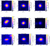 |
Fig. 1 ALMA pipeline-produced integrated intensity maps (color scale) with the line channels excluded, which are dominated by dust emission, for the studied sample of sources. On-source spectra are extracted by averaging the flux from the pixels within the circular area centered on “X.” |
3.1 IRAS 16293-2422 B
Towards IRAS 16293 B, the main S-bearing species (H2S and OCS, 1 = 0) and all the targeted minor isotopologs were securely detected, except for HDS due to a very high Eup value (1277 K) and the double isotopologs of HD34S,18OC34S,18O13CS, due to their low abundances (and high Eup for the case of HD34S). The detected transitions of H2S, 22,0−21,1 and OCS, υ = 0, J = 19–18 are bright and optically thick (τ ≫ 1). The  S line is marginally optically thick (τ = 0.2), as shown in Fig. 3. The vibrationally excited OCS, υ2 = 1± lines were detected. The lines of the detected molecules do not suffer from blending, except the
  S, 22,0,3−21,1,3 transition at 215.512 GHz, which is contaminated by the CH3CHO, 112,9−102,8 transition. HD34S, 73,4−73,5 transition at 232.964 GHz is heavily blended with the CH3CN, υ8 = 1, J = 15–15, K = 7−5 transition. It is most likely that all the emission seen around the rest frequency of HD34S comes from CH3CN, because HD34S is a minor species (32S/34S = 22, Wilson 1999, and D/H ~ 0.04 incl. the statistical correction by a factor of 2 to account for the two indistinguishable D atom positions, Drozdovskaya et al. 2018) and the Eup of this transition is high (416 K). The spectra of detected and undetected lines are in Figs. B.1 and B.2, respectively.
For the analysis of the targeted S-bearing molecules toward IRAS 16293 B, a Tex value of 125 K is assumed. This value has been deduced to be the best-fitting on the basis of ALMA-PILS observations at higher spatial resolution obtained with the 12m array and a full inventory of S-bearing molecules (Drozdovskaya et al. 2018). A FWHM of 1 km s−1 was adopted, as it has been shown that this value consistently fits nearly all the molecules investigated toward the hot inner regions of IRAS 16293 B (e.g., Jørgensen et al. 2018). For the larger scales probed by the present ALMA ACA observations, a deviation by 2 km s−1 from this FWHM can be seen for optically thick lines. This broadening in FWHM is likely due to the opacity broadening effects, which are dominant in optically thick lines, but this can be neglected in optically thin lines (Hacar et al. 2016). The synthetic spectral fitting has been carried out for two potential source sizes, 1″ and 2″ (Table 4). Column densities depend on the assumed source size and are lower for the larger source size. However, the N(H2S)/N(OCS) ratio is 1.3±0.27 and 1.3±0.28 for source sizes of 1″ and 2″, respectively. Thus, the ratio is independent of the assumed source size and is robustly determined with the ALMA ACA data.
For a source size of 2″, the column density of the vibrationally excited state of OCS, υ2 = 1± derived for IRAS 16293 B (2.5×1016 cm−2) is an order of magnitude lower than the OCS, υ2 = 1 column density (2.0×1017 cm−2) derived in Drozdovskaya et al. (2018). For a source size of 1″, the value obtained here (8 5 × 1016 cm−2) is in closer agreement with Drozdovskaya et al. (2018). Likewise, the OCS, υ = 0 column density determined from the minor isotopologs of OCS for a source size of 1″ (2.7 × 1017 cm−2) is in a closer agreement with the column density of OCS, υ = 0 (2.8×1017 cm−2) derived in Drozdovskaya et al. (2018), also based on minor isotopologs than for source size of 2″ (7.0 × 1016 cm−2). Drozdovskaya et al. (2018) used a smaller source size (0.5″) to constrain the column densities of OCS and H2S. These comparisons suggest that the ALMA ACA observations in this work are subject to beam dilution, hence, the column densities are likely to be somewhat underestimated. The column density of H2S could not be constrained to better than a factor of 10 in Drozdovskaya et al. (2018), namely 1.6 × 10¹⁷–2.2 × 1018 cm−2. This was due to the fact that only deuterated isotopologs of H2S were covered by the PILS observations and the D/H ratio of H2S is only constrained to within a factor of 10. Based on values of the H2S column densities for 1″ and 2″ source sizes obtained in this work, the lower estimate for the H2S column density in Drozdovskaya et al. (2018) seems to be more accurate. In turn, the H2S/OCS ratio obtained in this work (1.3) is closer to the lower end of the 0.7–7 range computed in Drozdovskaya et al. (2018).
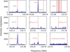 |
Fig. 2 Observed spectral windows of IRAS 16293-2422 B (Table 3) obtained with ALMA ACA at Band 6 frequencies (Table 1). A Doppler shift by υLSR = 2.7 km s−1 has been applied (Table 2). |
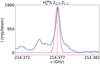 |
Fig. 3
|

3.2 Line profiles
For the synthetic spectral modeling, Gaussian line profiles were assumed (Sect. 2.3). However, even for optically thin lines, a deviation from Gaussian line profiles is seen in some cases. Two prominent examples are  S and O13CS in IRAS 16293 A (Fig. C.1), where the high spectral resolution of the data set clearly allows multiple peaks to be spectrally resolved in these lines. Likely, the reason for this is that this source is a compact binary (Maureira et al. 2020) with multiple components within the ACA beam of these observations. Another prominent example is the OCS, υ = 0 line in Ser-SMM3 (Fig. J.1), which has a double-peaked profile centered around the source velocity. Such a line profile is typical for a rotating structure around its protostar (which could resemble an envelope or disk in nature). Detailed modeling of line profiles is out of scope of this paper, as additional observations would be necessary in order to achieve meaningful results. For the purpose of studying the H2S/OCS ratio, these effects are secondary and likely do not significantly affect the calculated ratio and the conclusions of this paper. For IRAS 16293 A, the column density of
  S is not used to get the column density of H2S, because it is computed to be partially optically thick. Meanwhile, the column density of OCS as obtained from O13CS is within a factor of 2 of what is obtained from OC33S and 18OCS. For Ser-SMM3, the lack of constraints on the excitation temperature dominates the uncertainty in the H2S/OCS ratio.
H2S/OCS ratio for the studied sources, including their evolutionary class, binarity, environment, and the derived column densities of H2S and OCS for the stated excitation temperatures.
3.3 H2S/OCS ratio determination
The column densities of H2S and OCS derived on the basis of ALMA ACA observations have been used to constrain the ratio of H2S to OCS (Table 5). It was possible to compute this ratio for five out of ten sources in the considered sample. Neither H2S nor OCS were detected in Emb-25 and TMC1, consequently, the H2S/OCS ratio could not be constrained. The non-detection of OCS in IRS7B allowed us to derive only a lower limit on the H2S/OCS ratio. Table 5 also contains the best-available estimates of the H2S/OCS ratio for the warm and cold components of B1-c, and for the cold component of BHR71-IRS1, although these numbers carry a higher level of uncertainty due to line opacity that could not be resolved on the basis of these observations. For the warm component of BHR71-IRS1, a lower limit on the H2S/OCS ratio could be computed. For further analysis, the sample has been divided into three sub-samples: compact binary, wide binary, and single, based on the separations between components of multiple sources or closest neighbors.
4 Discussion
Figure 4 displays the derived protostellar H2S/OCS ratios, as well as the cometary (67P/Churyumov-Gerasimenko, hereafter 67P/C-G) and interstellar ice (W33A and Mon R2 IRS2) H2S/OCS ratios. The derived protostellar H2S/OCS ratios span a range from 0.2 to above 9.7. The ratios show a variation of approximately one order of magnitude, being the lowest in IRAS 16293 A and SMM3, and the highest in BHR71-IRS1.
In Sects. 4.1 and 4.2, we make a comparison of the protostellar H2S/OCS ratios with this ratio in interstellar and cometary ices, respectively. Comets are thought to preserve the chemical composition of the Sun’s birth cloud (Mumma & Charnley 2011). By comparing the H2S/OCS ratio of comet 67P/C-G with the ratios in nascent solar-like protostellar systems, an assessment can be made whether such an inheritance is true in the case of S-bearing molecules.
4.1 Interstellar ices
Observations toward the cold, outer protostellar envelopes of high-mass protostars W33A and Mon R2 IRS2 are used to acquire the H2S/OCS ratio in interstellar ices. The ratio is computed based on the ice abundances of OCS detected as an absorption feature at 4.9 µm (Palumbo et al. 1995) using the Infrared Telescope Facility (IRTF) and the upper limits on the H2S abundance derived based on the non-detection of the 3.98 µm band. The column density of solid OCS with respect to solid H2O is Nsolid(OCS)/Nsolid(H2O) = 4×10⁻⁴ (Palumbo et al. 1995) and Nsolid(OCS)/Nsolid(H2O) = 5.5×10⁻⁴ (Palumbo et al. 1997) for W33A and Mon R2 IRS2, respectively. Based on the non-detection of solid H2S toward W33A in the Infrared Space Observatory (ISO) Spectra from the Short Wavelength Spectrometer (SWS), NSolid(H2S)/Nsolid(H2O)Solid <0·03 (van der Tak et al. 2003). The upper limits on the solid H2S and solid H2O in Mon R2 IRS2 are < 0.2 × 10¹⁷ and 42.7 × 1017 cm−2 (Smith 1991), respectively, yielding NSolid(H2S)/NSolid(H2O) < 4.7×10⁻³. The H2S/OCS ratio in interstellar ices is poorly constrained due to the non-detection of solid H2S to date. The upper limits on the interstellar ices ratio are within the uncertainties of the cometary ices ratio. The derived protostellar ratios for all the sources are lower than the upper limit on the H2S/OCS ratio determined for interstellar ices - except BHR71-IRS1, with the H2S/OCS ratio exceeding the upper limit on the ratio for Mon R2 IRS2.
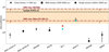 |
Fig. 4 N(H2S)/N(OCS) of the studied sources. Different symbols represent different types of sources: “star” for close binary (<500 au), “square” for wide binary (500–5000 au), and “circle” for single sources (within 5000 au). The upper limits on the interstellar ice (W33A and Mon R2 IRS2) ratios are shown by downward arrows. The uncertainty on the H2S/OCS ratio in comet 67P/C-G is shown by the coral shaded region. The lower limit on the ratio in IRS7B is shown by an upwards arrow. The H2S/OCS ratios for the cold (cyan) and warm (orange) components of Bl-c, and cold (cyan) component of BHR7l -1RS 1 are the best-available estimates pending opacity issues. These latter three data points do not have error bars associated to them in the figure (so as to indicate that they are merely estimates). |
4.2 Comet 67P/Churyumov-Gerasimenko
Comets are thought to be the most unprocessed objects in the Solar System (Mumma & Charnley 2011). Cometary chemical composition has been shown to be similar to a degree to that of star-forming regions (Bockelée-Morvan et al. 2000; Drozdovskaya et al. 2019). Consequently, the cometary H2S/OCS ratio is thought to provide an independent measurement of this ratio in interstellar ices. The H2S and OCS abundances from the ESA Rosetta mission were used to compute the H2S/OCS ratio for the Jupiter-family comet 67P/C-G. The H2S and OCS abundances relative to H20 are 1.10±0.46% and  , respectively (Rubin et al. 2019). These molecules are typical constituents of comets (Lis et al. 1997; Bockelée-Morvan et al. 2000; Boissier et al. 2007; Mumma & Charnley 2011). BHR71-IRS1 is the only protostar in the sample with a H2S/OCS ratio within the uncertainties of the cometary ices ratio. The H2S/OCS ratio for the other sources is at least an order of magnitude lower than for 67P/C-G, while even considering the high uncertainties on the cometary value. The availability of H2S relative to H2O in cometary ice (0.0064–0.0156) appears to be higher than in the interstellar ices toward Mon R2 IRS2 (<0.0047). For W33A, the currently available upper limit (<0.03) is less constraining and, hence, no conclusion can be drawn about how its ices compare to those of comet 67P/C-G. The relative ratio of H2S to OCS is only one window onto the inventory of S-bearing molecules in gas and ice at different stages of star and planet formation, meanwhile the overall availability relative to, for example, H2O is another window that requires dedicated exploration.
4.3 H2S/OCS ratio as an environmental (clustered or isolated) tracer
The measured gas-phase H2S/OCS ratios in the sample of young, low-mass protostars explored in this paper are predominantly lower (by as much as an order of magnitude) than the solid-state ratio measured through direct infrared observations of interstellar ices and indirectly via comets (Fig. 4). There appears to be no correlation with binarity nor a specific host cloud (Table 5). The dependence with evolutionary stage could not be properly explored, as the sample contains only one Class I source (TMC1), which did not result in detections of neither H2S nor OCS.
The highest ratio of ≥9.7 is found for the warm component (250 K) of BHR71-IRS1, which is a wide binary (~3 200 au; Bourke 2001; Parise et al. 2006; Chen et al. 2008; Tobin et al. 2019) Class 0 protostar. The ratio in BHR71-IRS1 resides within the uncertainty of the cometary ratio, but is between the two upper limits derived for the interstellar ices. The overall envelope mass and bolometric luminosity of BHR71-IRS1 is comparable to those of other compact binary and wide binary systems. The similarity of its gas-phase H2S/OCS ratio to the ratio in ices may suggest that it is displaying the most recently thermally desorbed volatiles that have not been subjected to gas-phase processing for long. However, what makes BHR71-IRS1 stand out is that it is located in an isolated cloud, namely, it is not associated with processes typical for clustered environments such as dynamical interactions, mechanical and chemical feedback from outflows, or enhanced irradiation.
It is possible that isolation resulted in lower irradiation of the ice grains during the prestellar phase in BHR71-IRS1, thus converting less H2S ices to OCS ices by photodissociation in the presence of CO ice. Consequently, leaving a higher H2S/OCS ratio in ices, which after evaporation resulted in a higher H2S/OCS ratio in the gas phase. Another reason could be more efficient hydrogenation chemistry in such a colder environment. On dust grains, hydrogenation is expected to be the most effective process leading to the formation of H2S (Wakelam et al. 2011; Esplugues et al. 2014). Hence, BHR71-IRS1 may have a higher H2S content and a lower OCS content, which results in a higher H2S/OCS ratio. Water deuteration is also higher by a factor of 2–4 in isolated protostars such as BHR71-IRS1 in comparison to those in clustered environments, such as IRAS 16293 and IRAS4 (Jensen et al. 2019).
One alternative cause of lower H2S/OCS ratios toward clustered low-mass protostars could be local temperature differences in their birth clouds, for instance, due to enhanced irradiation from the neighbouring protostars. Laboratory experiments have proven that OCS forms readily in ices when interstellar iceanalogs are irradiated by high-energy photons (Ferrante et al. 2008; Garozzo et al. 2010; Jiménez-Escobar & Muñoz Caro 2011; Chen et al. 2015). This would lead to a lower H2S/OCS ratio.
Additionally, cosmic rays and other forms of radiation (UV and X-ray photons) are a ubiquitous source of ionization in the interstellar gas. It is a pivotal factor in the dynamical and chemical evolution of molecular clouds (Padovani et al. 2018, 2020). Cosmic rays are not attenuated in the molecular clouds as strongly as UV photons (Ivlev et al. 2018; Padovani et al. 2018; Silsbee et al. 2018). Thus, dust grains in the interstellar medium can be heated by impinging cosmic rays, thereby heating up the icy grain mantles and resulting in calamitous explosions (Leger et al. 1985; Ivlev et al. 2015) and activating chemistry in solids (Shingledecker et al. 2017). Magnetohydrodynamic simulations have shown a higher cosmic ray production in protostars in a clustered environment (Kuffmeier et al. 2020), which would be consistent with the lower H2S/OCS ratios for such protostars found in this work. The results suggest that the H2S/OCS ratio traces the environment (isolated or clustered) of the protostellar systems. However, a follow-up study is needed as the sample consisted of only one isolated source.
5 Conclusions
In this work, we probe a sample of ten low-mass protostars for the presence of H2S, OCS, and their isotopologs using ALMA ACA Band 6 observations. For 5 out of 10 protostars, the H2S/OCS ratio was firmly constrained, and for an additional 3, best-possible estimates were obtained. This ratio is thought to be a potential chemical and physical clock of star-forming regions, which sheds light on the sulfur depletion that transpires from the diffuse medium to the dense core stage. Our main conclusions are:
The main S-bearing species, H2S and OCS, are detected in IRAS 16293-2422 A, IRAS 16293-2422 B, NGC 1333-IRAS4A, NGC 1333-IRAS4B, Per-B1-c, BHR71-IRS1, and Ser-SMM3. There are 1-σ upper limits on the column densities of OCS derived for RCrA IRS7B, TMC1, and Per-emb-25; and 1-σ upper limits on the column densities of H2S are derived for TMC1 and Per-emb-25;
The gas-phase H2S/OCS ratio ranges from 0.2 to above 9.7, and is typically at least one order of magnitude lower than that of ices. The lowest ratio is obtained for IRAS 16293 A and Ser-SMM3, while the highest is for BHR71-IRS1. The environment of the natal cloud, prior to the onset of star formation, may have played a major role in the distribution of sulfur across various S-bearing molecules, which have resulted in a spread in the H2S/OCS ratio by one order of magnitude;
The upper limits derived for the interstellar ices (Mon R2 IRS2 and W33A) lie within the uncertainties of the cometary ices ratio, specifically, that of comet 67P/Churyumov-Gerasimenko. The protostellar ratios are lower than the upper limits on the interstellar ices ratio and the cometary ices ratio by at least one order of magnitude for all sources, except BHR71-IRS1;
The lower ratio in clustered protostellar regions could be due to elevated birth cloud temperatures or due to additional radiation from nearby protostars, thereby enhancing the photodissociation pathways from H2S to OCS;
The high H2S/OCS ratio in BHR71-IRS1 could be the result of less efficient photodissociation of H2S to OCS in the presence of CO ice in its isolated birth cloud or more efficient hydrogenation chemistry leading to more efficient H2S formation.
Follow-up high spatial resolution observations are required toward several sources to better constrain the spatial distribution and excitation temperatures associated with the H2S and OCS detections. Furthermore, the difference of more than tenfold in the H2S/OCS ratio toward Class 0 protostars in clustered and isolated environments is a strong motivation for performing more spectroscopic observations toward such sources, thereby understanding the physical and chemical differences in the two types of environments. Observations from James Webb Space Telescope (JWST) could play an important role in constraining the H2S/OCS ice ratio in low- and intermediate-mass stars. More studies of the H2S/OCS ratio in a larger sample of Class 0 and Class I protostars in clustered and isolated environments should also be performed to further understand the sulfur chemistry in star-forming regions.
Acknowledgements
The research was started as part of the Leiden/ESA Astrophysics Program for Summer Students (LEAPS) 2021. M.N.D. acknowledges the support by the Swiss National Science Foundation (SNSF) Ambizione grant no. 180079, the Center for Space and Habitability (CSH) Fellowship, and the IAU Gruber Foundation Fellowship. This paper makes use of the following ALMA data: ADS/JAO.ALMA#2017.1.00108.S and ADS/JAO.ALMA#2017.1.01350.S. ALMA is a partnership of ESO (representing its member states), NSF (USA) and NINS (Japan), together with NRC (Canada), MOST and ASIAA (Taiwan), and KASI (Republic of Korea), in cooperation with the Republic of Chile. The Joint ALMA Observatory is operated by ESO, AUI/NRAO and NAOJ. This research made use of Astropy, a community-developed core Python package for Astronomy (Astropy Collaboration 2013, 2018; http://www.astropy.org). The authors would like to thank Prof. Dr. Ewine van Dishoeck for useful discussions about the H2S/OCS ratio, and the anonymous referee for constructive feedback.
Appendix A Inventory of targeted sources and detected and undetected emission lines
Lines of H2S, OCS, and their isotopologs towards the targeted sources. The columns show 1) the CDMS entry, 2) the quantum numbers associated to the transition, 3) the rest frequency of the line, 4) the upper energy level of the transition, 5) the Einstein A coefficient of the transition, and the line evaluation done for different protostars given in columns 6-14.
Appendix B IRAS 16293-2422 B
The synthetic spectral fitting of the detected species toward IRAS 16293 B is presented thoroughly in Section 3.1. An extensive study of the effect of source size on column density and H2S/OCS is also presented in Section 3.1. The excitation temperature and FHWM assumed for fitting synthetic spectra to the detected lines toward IRAS 16293 B are 125 K and 1 km s−1, respectively, based on the ALMA-PILS observations of IRAS 16293 (Drozdovskaya et al. 2018).
Appendix B.1 Detected lines in IRAS 16293-2422 B
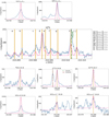 |
Figure B.1 Observed spectra (in blue), rest frequency of the detected line (brown dashed line), spectroscopic uncertainty on the rest frequency of the detected line (yellow shaded region), blending species (green dash-dotted line and red dashed line), and fitted synthetic spectra (in pink) plotted for the sulfur-bearing species detected toward IRAS 16293-2422 B. |


Appendix B.2 Undetected lines in IRAS 16293-2422 B
 |
Figure B.2 Observed spectra (in blue), rest frequency of the undetected line (brown dashed line), and spectroscopic uncertainty on the rest frequency of the undetected line (yellow shaded region) plotted for the sulfur-bearing species undetected toward IRAS 16293-2422 B. |
Appendix C IRAS 16293-2422 A
The strengths of the lines detected toward IRAS 16293 A are comparable to those toward IRAS 16293 B. The lines of H2S, 22,0 - 21,1 and OCS, υ = 0, J= 19-18 are bright and optically thick (τ≫1). The line of  S is marginally optically thick (τ= 0.1). For the analysis of IRAS 16293 A, we have assumed Tex = 125 K, which is typical for the hot inner regions of this source (Calcutt et al. 2018; Manigand et al. 2020), and a source size of 2″ in diameter (based on the investigation of IRAS 16293 B; Section 3.1). The fitted FWHM and N, and the computed τ are given in Table C.1 for the detected S-bearing molecules. Due to the high spectral resolution of the data, all detected lines are spectrally resolved to be double- or multi-peaked. This is possibly caused by the multiple components of the compact binary IRAS 16293 A (Maureira et al. 2020). One of the detected
  S lines (at 215.512 GHz) is contaminated by the CH3CHO molecule. The line of HD34S is heavily blended with that of CH3CN, υ8 = 1 at 232.965 GHz. Having 32S/34S=22 (Wilson 1999) and D/H ~0.04 (incl. statistical correction; Drozdovskaya et al. 2018), it is most likely that all the emission seen around the rest frequency of HD34S stems from CH3CN. The spectra of detected and undetected molecules can be found in Figure C.1 and Figure C.2, respectively.
Synthetic fitting of the detected S-bearing species toward IRAS 16293-2422 A for an excitation temperature (Tex) of 125 K and a source size of 2″. Directly across from a specific minor isotopolog under “Derived N of isotopologs” follows the column density of the main isotopolog upon the assumption of the standard isotopic ratio. In bold in the same column, we show the average column density of the main isotopolog based on all the available minor isotopologs (only if the minor isotopolog is optically thin and including the uncertainties).
Appendix C.1 Detected lines in IRAS 16293-2422 A
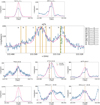 |
Figure C.1 Observed spectra (in blue), rest frequency of the detected line (brown dashed line), spectroscopic uncertainty on the rest frequency of the detected line (yellow shaded region), blending species (green dash-dotted line and red dashed line), and fitted synthetic spectra (in pink) plotted for the sulfur-bearing species detected toward IRAS 16293-2422 A. |


Appendix C.2 Undetected lines in IRAS 16293-2422 A
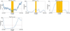 |
Figure C.2 Observed spectra (in blue), rest frequency of the undetected line (brown dashed line), and spectroscopic uncertainty on the rest frequency of the undetected line (yellow shaded region) plotted for the sulfur-bearing species undetected toward IRAS 16293-2422 A. |
Appendix D NGC 1333-IRAS4A
Line detections in IRAS4A are nearly the same as in IRAS 16293 A and IRAS 16293 B. The main sulfur species, H2S, 22,0-21,1 and OCS, υ = 0, J = 19 − 18, are bright and optically thick, τ>1 for 50 ≤ Tex < 200 K or partially optically thick, 0.1 ≤ τ < 1 for Tex ≥200 K. The two protostars in IRAS4A, 4A1 and 4A2, could not be disentangled due to insufficient angular resolution of the ALMA ACA observations toward this source in comparison to the separation between the two components (1.8″, i.e., 540 au; Sahu et al. 2019). Due to a lack of small-scale constraints on the distribution of S-bearing molecules in IRAS4A, a range of excitation temperature between 150 and 300 K is considered (López-Sepulcre et al. 2017). Temperatures of 50 and 100 K have been ruled out on the grounds that the observed signal at the frequency corresponding to the OCS, υ2 = 1± is incompatible with these lowest temperatures for column densities in the physical range of values. Looking at high spatial resolution maps from Sahu et al. (2019), a 2″ source size is assumed to cover the circumbinary envelope around 4A1 and 4A2. The spectra fitted to the line profiles have a FWHM of 1.8 km s−1. The computed column densities of the detected species are reported in Table D.1 for excitation temperatures in the 150 – 300 K range. The lines of  and HD34S face the same blending effects as in IRAS 16293 A and IRAS 16293 B.
Appendix D.1 Results of the synthetic fitting of the line profiles toward NGC 1333-IRAS4A for Tex = 150 – 300 K
Synthetic fitting of the detected S-bearing species toward NGC 1333-IRAS4A for a range of excitation temperatures between 150 and 300 K, a FWHM of 1.8″, and a source size of 2″. Directly across from a specific minor isotopolog under “Derived N of isotopologs” follows the column density of the main isotopolog upon the assumption of the standard isotopic ratio. In bold in the same column is the average column density of the main isotopolog based on all the available minor isotopologs (only if the minor isotopolog is optically thin and including the uncertainties).
Appendix D.2 Detected lines in NGC 1333-IRAS4A
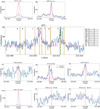 |
Figure D.1 Observed spectra (in blue), rest frequency of the detected line (brown dashed line), spectroscopic uncertainty on the rest frequency of the detected line (yellow shaded region), blending species (green dash-dotted line and red dashed line), and fitted synthetic spectra (in pink) plotted for the sulfur-bearing species detected toward NGC 1333-IRAS4A for Tex = 150 K. |


Appendix D.3 Undetected lines in NGC 1333-IRAS4A
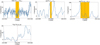 |
Figure D.2 Observed spectra (in blue), rest frequency of the undetected line (brown dashed line), and spectroscopic uncertainty on the rest frequency of the undetected line (yellow shaded region) plotted for the sulfur-bearing species undetected toward NGC 1333-IRAS4A. |
Appendix E RCrA IRS7B
H2S, 22,0-21,1 is the only emission line detected toward IRS7B (Figure E.1). The synthetic spectrum for this line is best-fitted for a FWHM of 1 km s−1, an excitation temperature of 100 K, and a source size of 1.5″, as determined from ALMA 12m observations (project id: 2017.1.00108.S; PI: M. N. Drozdovskaya) toward IRS7B. The upper limit on the column density of OCS, υ = 0 is stated in Table 5 and E.1. IRS7B exhibits weak hot corino activity, resulting in few detections of complex organic molecules and their low abundances (Lindberg et al. 2015). The chemical composition in the envelope of IRS7B could be affected by the enhanced UV radiation (photodissociation) from the nearby Herbig Ae star RCrA located at a distance of 39″ (6 630 au) NW of IRS7B (Watanabe et al. 2012).
Synthetic fitting of the detected S-bearing species toward RCrA IRS7B for an excitation temperature of 100 K, FWHM of 1 km s−1, and source size of 1.5″.
Appendix E.1 Detected lines in RCrA IRS7B
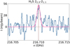 |
Figure E.1 Observed spectrum (in blue), rest frequency of the detected line (brown dashed line), spectroscopic uncertainty on the rest frequency of the detected line (yellow shaded region), and fitted synthetic spectrum (in pink) plotted for the sulfur-bearing species detected toward RCrA IRS7B. |
Appendix E.2 Undetected lines in RCrA IRS7B
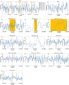 |
Figure E.2 Observed spectra (in blue), rest frequency of the undetected line (brown dashed line), and spectroscopic uncertainty on the rest frequency of the undetected line (yellow shaded region) plotted for the sulfur-bearing species undetected toward RCrA IRS7B. Synthetic spectrum (in pink) fitted to the OCS, υ = 0 line with the 1-σ upper limit on its column density. |
Appendix F B1-c
H2S, 22,0-21,1 and OCS, υ = 0, J = 19 − 18 lines are detected toward B1-c. Unfortunately, no optically thin isotopologs of H2S and OCS were observed toward B1-c in this observational data set. Synthetic spectra for the detected H2S and OCS lines are fitted for two components of B1-c, a cold component (Tex = 60 K) and a warm central component (Tex = 200 K) for a source size of 0.45″ (as assumed in van Gelder et al. 2020 for the same observations). The best-fitting FWHM is 2.2 km s−1. The fitting parameters, computed N and τ values are tabulated in Table F.1 and F.2. For the cold component, the H2S line is optically thick (τ=2.0); whereas the OCS, υ = 0, J = 19−18 line is partially optically thick (τ = 0.7). For the warm component, both H2S and OCS, υ = 0 lines are partially optically thick (τ = 0.26 and τ = 0.10, respectively). The undetected lines are shown in Figure F.3.
Synthetic fitting of the detected S-bearing species toward B1-c for the cold component (Tex = 60 K), a FWHM of 2.2 km s−1 and a source size of 0.45″.
Synthetic fitting of the detected S-bearing species toward B1-c for the warm component (Tex = 200 K), a FWHM of 2.2 km s−1, and a source size of 0.45″.
Appendix F.1 Detected lines in B1-c
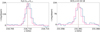 |
Figure F.1 Observed spectra (in blue), rest frequency of the detected line (brown dashed line), spectroscopic uncertainty on the rest frequency of the detected line (yellow shaded region), and fitted synthetic spectra (in pink) plotted for the sulfur-bearing species detected toward the cold component (Tex = 60 K) of B1-c. |
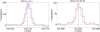 |
Figure F.2 Observed spectra (in blue), rest frequency of the detected line (brown dashed line), spectroscopic uncertainty on the rest frequency of the detected line (yellow shaded region), and fitted synthetic spectra (in pink) plotted for the sulfur-bearing species detected toward the warm component (Tex = 200 K) of B1-c. |
Appendix F.2 Undetected lines in B1-c
 |
Figure F.3 Observed spectra (in blue), rest frequency of the undetected line (brown dashed line), and spectroscopic uncertainty on the rest frequency of the undetected line (yellow shaded region) plotted for the sulfur-bearing species undetected toward B1-c. |
Appendix G BHR71-IRS1
H2S, 22,0-21,1 and OCS, υ = 0, J = 19−18 emission lines are detected toward BHR71-IRS1 (Figure G.1, G.2). As for B1-c, two excitation temperatures (100 and 250 K) probing two different regions are inputted into the modeling of synthetic spectra for BHR71-IRS1. The excitation temperatures are taken from the detection of methanol at Tex = 100 K and gauche-ethanol at Tex = 250 K (Yang et al. 2020). Yang et al. (2020) fitted CS for a source size of 0.32″; however, in order to cover a larger area of the envelope a source size of 0.6″, and a FWHM of 2.5 km s−1 is assumed here. The H2S line of the colder component seems to be optically thick (τ = 1.8), while the OCS, υ = 0 line is partially optically thick for this component (τ = 0.23). H2S is partially optically thin for the warmer component (τ = 0.39). The spectra of the undetected lines are shown in Figure G.3.
Synthetic fitting of the detected S-bearing species toward BHR71-IRS1 for an excitation temperature of 100 K, FWHM of 2.5 km s−1 and source size of 0.6″.
Synthetic fitting of the detected S-bearing species toward BHR71-IRS1 for an excitation temperature of 250 K, FWHM of 2.5 km s−1 and source size of 0.6″.
Appendix G.1 Detected lines in BHR71-IRS1
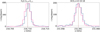 |
Figure G.1 Observed spectra (in blue), rest frequency of the detected line (brown dashed line), spectroscopic uncertainty on the rest frequency of the detected line (yellow shaded region), and fitted synthetic spectra (in pink) plotted for the sulfur-bearing species detected toward the cold component (Tex = 100 K) of BHR71-IRS1. |
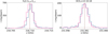 |
Figure G.2 Observed spectra (in blue), rest frequency of the detected line (brown dashed line), spectroscopic uncertainty on the rest frequency of the detected line (yellow shaded region), and fitted synthetic spectra (in pink) plotted for the sulfur-bearing species detected toward the warm component (Tex = 250 K) of BHR71-IRS1. |
Appendix G.2 Undetected lines in BHR71-IRS1
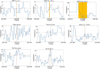 |
Figure G.3 Observed spectra (in blue), rest frequency of the undetected line (brown dashed line), and spectroscopic uncertainty on the rest frequency of the undetected line (yellow shaded region) plotted for the sulfur-bearing species undetected toward BHR71-IRS1. |
Appendix H Per-emb-25
No S-bearing species are detected toward Emb-25. Consequently, 1-σ upper limits on the column densities of H2S and OCS, υ = 0 are computed assuming a source size of 1″ (Yang et al. 2021), a FWHM of 1 km s−1, and excitation temperatures in the range of 50 – 300 K. The upper limits on H2S and OCS, υ = 0 column densities are < 8.3 × 10¹³ and ≤ 3.2 × 1014 cm−2, respectively (Table 5 and H.1). The spectra of all the undetected species are presented in Figure H.1.
Appendix H.1 1 -σ upper limits on the column densities of H2S and OCS, υ = 0 of Per-emb-25
Synthetic fitting of the non-detected main S-bearing species toward Per-emb-25 for a range of excitation temperatures between 50 and 300 K, a FWHM of 1 km s−1, and a source size of 1″.
Appendix H.2 Undetected lines in Per-emb-25
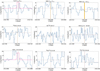 |
Figure H.1 Observed spectra (in blue), rest frequency of the undetected line (brown dashed line), and spectroscopic uncertainty on the rest frequency of the undetected line (yellow shaded region) plotted for the sulfur-bearing species undetected toward Per-emb-25. Synthetic spectra (in pink) fitted to H2S and OCS, υ = 0 lines with the 1-σ upper limit on their column densities. |
Appendix I NGC 1333-IRAS4B
H2S, OCS, υ = 0, J = 19 − 18, and OC33S, J = 18 − 17 emission lines are detected in IRAS4B. Initially, an excitation temperature and a source size of 210 K and 2″, respectively, were assumed for the modeling based on the rotation temperature of the detected CH3OH lines toward this source (Yang et al. 2021). In this case, the computed τ values indicate that all the lines are optically thin (Table I.1). However, there is a mismatch by an order of magnitude in the column density of OCS, as determined from its υ = 0 line and the OC33S line. It is unlikely that the isotopic ratio of 32S/33S deviates from the canonical value for this one source in the well-studied NGC 1333. It is more likely that the assumed source size and excitation temperature are not appropriate for OCS (and H2S by extension). An exploration of the parameter space demonstrated that an excitation temperature of 100 K and a source size of 1″ are more appropriate for these S-bearing molecules (Table I.2). In this case, the OCS, υ = 0 line is partially optically thick and thus the column density determined from its optically thin minor OC33S isotopolog is more reliable. The fitted synthetic spectra and spectra of undetected species are shown in Figure I.1 and Figure I.2, respectively. Figure I.1 shows that the lines of S-bearing molecules deviate from the literature υLSR = 7.4 km/s value that was determined based on CO observations Kristensen et al. (2012). A single υLSR value does not fit all the emission lines detected in this work. This discrepancy can only be understood with a more thorough characterisation of the structure of this source on large and small spatial scales.
Synthetic fitting of the detected S-bearing species toward NGC 1333-IRAS4B for an excitation temperature of 210 K and a source size of 2″. Directly across from a specific minor isotopolog under “Derived N of isotopologs” follows the column density of the main isotopolog upon the assumption of the standard isotopic ratio.
Synthetic fitting of the detected S-bearing species toward NGC 1333-IRAS4B for an excitation temperature of 100 K and a source size of 1″. Directly across from a specific minor isotopolog under “Derived N of isotopologs’ follows the column density of the main isotopolog upon the assumption of the standard isotopic ratio.
Appendix I.1 Detected lines in NGC 1333-IRAS4B
 |
Figure I.1 Observed spectra (in blue), rest frequency of the detected line (brown dashed line), spectroscopic uncertainty on the rest frequency of the detected line (yellow shaded region), and fitted synthetic spectra (in pink) plotted for the sulfur-bearing species detected toward NGC 1333-IRAS4B for Tex = 100 K and a source size of 1″. |
Appendix I.2 Undetected lines in NGC 1333-IRAS4B
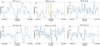 |
Figure I.2 Observed spectra (in blue), rest frequency of the undetected line (brown dashed line), and spectroscopic uncertainty on the rest frequency of the undetected line (yellow shaded region) plotted for the sulfur-bearing species undetected toward NGC 1333-IRAS4B. |
Appendix J Ser-SMM3
The excitation temperature was difficult to estimate for SMM3, as no molecular tracer of the inner envelope has been detected. As a result, the column density of the detected H2S, 22,0-21,1 and OCS, υ = 0, J = 19 − 18 lines is evaluated for a range of excitation temperatures between 100 and 250 K. The OCS, υ = 0 line shows a double peaked feature and the synthetic spectrum is fitted covering both peaks. The best-fitting models to H2S and OCS, υ = 0 have line widths of 2.5 and 3.0 km s−1, and source sizes of 2.0″ and 0.5″, respectively. Different source sizes for H2S and OCS were assumed in this source, because 12m ALMA data at a spatial resolution of 0.5″ show very different spatial distributions for these molecules. The H2S and OCS integrated intensity maps in fig. 9 of Tychoniec et al. (2021) show extended emission for H2S covering ~2″ and much more compact emission for OCS ~0.5″. The lines are optically thin (τ < 0.1) with line opacities tabulated in Table J.1.
Synthetic fitting of the detected S-bearing species toward Ser-SMM3 for a range of excitation temperatures between 100 and 250 K.
Appendix J.1 Detected lines in Ser-SMM3
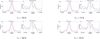 |
Figure J.1 Observed spectra (in blue), rest frequency of the detected line (brown dashed line), spectroscopic uncertainty on the rest frequency of the detected line (yellow shaded region), and fitted synthetic spectra (in pink) plotted for the sulfur-bearing species detected toward Ser-SMM3 for a range of excitation temperature between 100 and 250 K. |
Appendix J.2 Undetected lines in Ser-SMM3
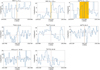 |
Figure J.2 Observed spectra (in blue), rest frequency of the undetected line (brown dashed line), and spectroscopic uncertainty on the rest frequency of the undetected line (yellow shaded region) plotted for the sulfur-bearing species undetected toward Ser-SMM3. |
Appendix K TMC1
No S-bearing species are detected toward TMC1. Thus, 1-σ upper limit on the column density of H2S, 22,0-11,1 and OCS, υ = 0, J = 19 − 18 are computed with a FWHM of 1 km s−1, for an excitation temperature of 40 K, and a source size of 1.5″ to include both the components of TMC1 (Harsono et al. 2014). The upper limits on the column density of H2S and OCS are given in the Table K.1. The undetected lines are shown in Figure K.1.
Synthetic fitting of the undetected main S-bearing species toward TMC1 for an excitation temperature of 40 K, FWHM of 1 km s−1, and source size of 1.5″.
Appendix K.1 Undetected lines in TMC1
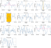 |
Figure K.1 Observed spectra (in blue), rest frequency of the undetected line (brown dashed line), and spectroscopic uncertainty on the rest frequency of the undetected line (yellow shaded region) plotted forthe sulfur-bearing species undetected toward TMC1. Synthetic spectra(in pink) fitted to the H2S, and the OCS, υ = 0 line with the 1-σ upper limit on its column density. |
References
- Agúndez, M., Marcelino, N., Cernicharo, J., & Tafalla, M. 2018, A&A, 611, A1 [NASA ADS] [CrossRef] [EDP Sciences] [Google Scholar]
- A’Hearn, M. F., Schleicher, D. G., & Feldman, P. D. 1983, ApJ, 274, L99 [CrossRef] [Google Scholar]
- Aikawa, Y., & Herbst, E. 1999, A&A, 351, 233 [NASA ADS] [Google Scholar]
- Aikawa, Y., Kamuro, D., Sakon, I., et al. 2012, A&A, 538, A57 [NASA ADS] [CrossRef] [EDP Sciences] [Google Scholar]
- Anderl, S., Maret, S., Cabrit, S., et al. 2016, A&A, 591, A3 [NASA ADS] [CrossRef] [EDP Sciences] [Google Scholar]
- Anderson, D. E., Bergin, E. A., Maret, S., & Wakelam, V. 2013, ApJ, 779, 141 [Google Scholar]
- Asplund, M., Grevesse, N., Sauval, A. J., & Scott, P. 2009, ARA&A, 47, 481 [NASA ADS] [CrossRef] [Google Scholar]
- Astropy Collaboration (Robitaille, T. P., et al.) 2013, A&A, 558, A33 [NASA ADS] [CrossRef] [EDP Sciences] [Google Scholar]
- Astropy Collaboration (Price-Whelan, A. M., et al.) 2018, AJ, 156, 123 [Google Scholar]
- Belloche, A., Maury, A. J., Maret, S., et al. 2020, A&A, 635, A198 [NASA ADS] [CrossRef] [EDP Sciences] [Google Scholar]
- Biver, N., Bockelée-Morvan, D., Boissier, J., et al. 2021a, A&A, 648, A49 [EDP Sciences] [Google Scholar]
- Biver, N., Bockelée-Morvan, D., Lis, D. C., et al. 2021b, A&A, 651, A25 [NASA ADS] [CrossRef] [EDP Sciences] [Google Scholar]
- Blake, G. A., Sutton, E. C., Masson, C. R., & Phillips, T. G. 1987, ApJ, 315, 621 [Google Scholar]
- Bockelée-Morvan, D., Lis, D. C., Wink, J. E., et al. 2000, A&A, 353, 1101 [Google Scholar]
- Boissier, J., Bockelée-Morvan, D., Biver, N., et al. 2007, A&A, 475, 1131 [NASA ADS] [CrossRef] [EDP Sciences] [Google Scholar]
- Boogert, A. C. A., Schutte, W. A., Helmich, F. P., Tielens, A. G. G. M., & Wooden, D. H. 1997, A&A, 317, 929 [NASA ADS] [Google Scholar]
- Boogert, A. C. A., Gerakines, P. A., & Whittet, D. C. B. 2015, ARA&A, 53, 541 [Google Scholar]
- Bourke, T. L. 2001, ApJ, 554, L91 [NASA ADS] [CrossRef] [Google Scholar]
- Brown, A. 1987, ApJ, 322, L31 [NASA ADS] [CrossRef] [Google Scholar]
- Brown, D. W., & Chandler, C. J. 1999, MNRAS, 303, 855 [NASA ADS] [CrossRef] [Google Scholar]
- Calcutt, H., Jørgensen, J. K., Müller, H. S. P., et al. 2018, A&A, 616, A90 [NASA ADS] [CrossRef] [EDP Sciences] [Google Scholar]
- Calmonte, U., Altwegg, K., Balsiger, H., et al. 2016, MNRAS, 462, S253 [NASA ADS] [CrossRef] [Google Scholar]
- Caux, E., Kahane, C., Castets, A., et al. 2011, A&A, 532, A23 [NASA ADS] [CrossRef] [EDP Sciences] [Google Scholar]
- Charnley, S. B. 1997, ApJ, 481, 396 [NASA ADS] [CrossRef] [Google Scholar]
- Chen, H., Myers, P. C., Ladd, E. F., & Wood, D. O. S. 1995, ApJ, 445, 377 [NASA ADS] [CrossRef] [Google Scholar]
- Chen, X., Launhardt, R., Bourke, T. L., Henning, T., & Barnes, P. J. 2008, ApJ, 683, 862 [NASA ADS] [CrossRef] [Google Scholar]
- Chen, Y. J., Juang, K. J., Nuevo, M., et al. 2015, ApJ, 798, 80 [Google Scholar]
- Codella, C., Bianchi, E., Podio, L., et al. 2021, A&A, 654, A52 [NASA ADS] [CrossRef] [EDP Sciences] [Google Scholar]
- Coutens, A., Vastel, C., Cabrit, S., et al. 2013, A&A, 560, A39 [NASA ADS] [CrossRef] [EDP Sciences] [Google Scholar]
- Davis, C. J., Matthews, H. E., Ray, T. P., Dent, W. R. F., & Richer, J. S. 1999, MNRAS, 309, 141 [NASA ADS] [CrossRef] [Google Scholar]
- De Simone, M., Ceccarelli, C., Codella, C., et al. 2020, ApJ, 896, L3 [NASA ADS] [CrossRef] [Google Scholar]
- Drozdovskaya, M. N., van Dishoeck, E. F., Jørgensen, J. K., et al. 2018, MNRAS, 476, 4949 [Google Scholar]
- Drozdovskaya, M. N., van Dishoeck, E. F., Rubin, M., Jørgensen, J. K., & Altwegg, K. 2019, MNRAS, 490, 50 [Google Scholar]
- Drozdovskaya, M. N., Coudert, L. H., Margulès, L., et al. 2022, A&A, 659, A69 [NASA ADS] [CrossRef] [EDP Sciences] [Google Scholar]
- Druard, C., & Wakelam, V. 2012, MNRAS, 426, 354 [NASA ADS] [CrossRef] [Google Scholar]
- Dzib, S. A., Ortiz-León, G. N., Hernández-Gómez, A., et al. 2018, A&A, 614, A20 [NASA ADS] [CrossRef] [EDP Sciences] [Google Scholar]
- Elias, J. H. 1978, ApJ, 224, 857 [NASA ADS] [CrossRef] [Google Scholar]
- Endres, C. P., Schlemmer, S., Schilke, P., Stutzki, J., & Müller, H. S. P. 2016, J. Mol. Spectrosc., 327, 95 [NASA ADS] [CrossRef] [Google Scholar]
- Enoch, M. L., Evans, I., Neal, J., Sargent, A. I., & Glenn, J. 2009, ApJ, 692, 973 [NASA ADS] [CrossRef] [Google Scholar]
- Esplugues, G. B., Viti, S., Goicoechea, J. R., & Cernicharo, J. 2014, A&A, 567, A95 [NASA ADS] [CrossRef] [EDP Sciences] [Google Scholar]
- Ferrante, R. F., Moore, M. H., Spiliotis, M. M., & Hudson, R. L. 2008, ApJ, 684, 1210 [NASA ADS] [CrossRef] [Google Scholar]
- Garozzo, M., Fulvio, D., Kanuchova, Z., Palumbo, M. E., & Strazzulla, G. 2010, A&A, 509, A67 [NASA ADS] [CrossRef] [EDP Sciences] [Google Scholar]
- Geballe, T. R., Baas, F., Greenberg, J. M., & Schutte, W. 1985, A&A, 146, L6 [NASA ADS] [Google Scholar]
- Goicoechea, J. R., Pety, J., Gerin, M., et al. 2006, A&A, 456, 565 [NASA ADS] [CrossRef] [EDP Sciences] [Google Scholar]
- Grim, R. J. A., & Greenberg, J. M. 1987, ApJ, 321, L91 [NASA ADS] [CrossRef] [Google Scholar]
- Hacar, A., Alves, J., Burkert, A., & Goldsmith, P. 2016, A&A, 591, A104 [NASA ADS] [CrossRef] [EDP Sciences] [Google Scholar]
- Harsono, D., Jørgensen, J. K., van Dishoeck, E. F., et al. 2014, A&A, 562, A77 [NASA ADS] [CrossRef] [EDP Sciences] [Google Scholar]
- Hatchell, J., Thompson, M. A., Millar, T. J., & MacDonald, G. H. 1998, A&A, 338, 713 [Google Scholar]
- Hatchell, J., Fuller, G. A., & Richer, J. S. 2007a, A&A, 472, 187 [NASA ADS] [CrossRef] [EDP Sciences] [Google Scholar]
- Hatchell, J., Fuller, G. A., Richer, J. S., Harries, T. J., & Ladd, E. F. 2007b, A&A, 468, 1009 [NASA ADS] [CrossRef] [EDP Sciences] [Google Scholar]
- Holdship, J., Viti, S., Jimenez-Serra, I., et al. 2016, MNRAS, 463, 802 [NASA ADS] [CrossRef] [Google Scholar]
- Howk, J. C., Sembach, K. R., & Savage, B. D. 2006, ApJ, 637, 333 [NASA ADS] [CrossRef] [Google Scholar]
- Ivlev, A. V., Röcker, T. B., Vasyunin, A., & Caselli, P. 2015, ApJ, 805, 59 [NASA ADS] [CrossRef] [Google Scholar]
- Ivlev, A. V., Dogiel, V. A., Chernyshov, D. O., et al. 2018, ApJ, 855, 23 [NASA ADS] [CrossRef] [Google Scholar]
- Jacobsen, S. K., Jørgensen, J. K., van der Wiel, M. H. D., et al. 2018, A&A, 612, A72 [NASA ADS] [CrossRef] [EDP Sciences] [Google Scholar]
- Jensen, S. S., Jørgensen, J. K., Kristensen, L. E., et al. 2019, A&A, 631, A25 [NASA ADS] [CrossRef] [EDP Sciences] [Google Scholar]
- Jiménez-Escobar, A., & Muñoz Caro, G. M. 2011, A&A, 536, A91 [Google Scholar]
- Jørgensen, J. K., Harvey, P. M., Evans, I., Neal, J., et al. 2006, ApJ, 645, 1246 [CrossRef] [Google Scholar]
- Jørgensen, J. K., Bourke, T. L., Nguyen Luong, Q., & Takakuwa, S. 2011, A&A, 534, A100 [NASA ADS] [CrossRef] [EDP Sciences] [Google Scholar]
- Jørgensen, J. K., van der Wiel, M. H. D., Coutens, A., et al. 2016, A&A, 595, A117 [Google Scholar]
- Jørgensen, J. K., Müller, H. S. P., Calcutt, H., et al. 2018, A&A, 620, A170 [Google Scholar]
- Kama, M., Shorttle, O., Jermyn, A. S., et al. 2019, ApJ, 885, 114 [Google Scholar]
- Keller, L. P., Hony, S., Bradley, J. P., et al. 2002, Nature, 417, 148 [Google Scholar]
- Köhler, M., Jones, A., & Ysard, N. 2014, A&A, 565, A9 [Google Scholar]
- Kristensen, L. E., van Dishoeck, E. F., van Kempen, T. A., et al. 2010, A&A, 516, A57 [NASA ADS] [CrossRef] [EDP Sciences] [Google Scholar]
- Kristensen, L. E., van Dishoeck, E. F., Bergin, E. A., et al. 2012, A&A, 542, A8 [NASA ADS] [CrossRef] [EDP Sciences] [Google Scholar]
- Kuffmeier, M., Zhao, B., & Caselli, P. 2020, A&A, 639, A86 [NASA ADS] [CrossRef] [EDP Sciences] [Google Scholar]
- Laas, J. C., & Caselli, P. 2019, A&A, 624, A108 [NASA ADS] [CrossRef] [EDP Sciences] [Google Scholar]
- Leger, A., Jura, M., & Omont, A. 1985, A&A, 144, 147 [Google Scholar]
- Li, J., Wang, J., Zhu, Q., Zhang, J., & Li, D. 2015, ApJ, 802, 40 [Google Scholar]
- Lindberg, J. E., Jørgensen, J. K., Brinch, C., et al. 2014, A&A, 566, A74 [NASA ADS] [CrossRef] [EDP Sciences] [Google Scholar]
- Lindberg, J. E., Jørgensen, J. K., Watanabe, Y., et al. 2015, A&A, 584, A28 [NASA ADS] [CrossRef] [EDP Sciences] [Google Scholar]
- Lis, D. C., Mehringer, D. M., Benford, D., et al. 1997, Earth Moon Planets, 78, 13 [NASA ADS] [CrossRef] [Google Scholar]
- Looney, L. W., Mundy, L. G., & Welch, W. J. 2000, ApJ, 529, 477 [NASA ADS] [CrossRef] [Google Scholar]
- López-Sepulcre, A., Sakai, N., Neri, R., et al. 2017, A&A, 606, A121 [NASA ADS] [CrossRef] [EDP Sciences] [Google Scholar]
- Manigand, S., Jørgensen, J. K., Calcutt, H., et al. 2020, A&A, 635, A48 [NASA ADS] [CrossRef] [EDP Sciences] [Google Scholar]
- Martín, S., Martín-Pintado, J., Mauersberger, R., Henkel, C., & García-Burillo, S. 2005, ApJ, 620, 210 [CrossRef] [Google Scholar]
- Matthews, B. C., Hogerheijde, M. R., Jørgensen, J. K., & Bergin, E. A. 2006, ApJ, 652, 1374 [NASA ADS] [CrossRef] [Google Scholar]
- Maureira, M. J., Pineda, J. E., Segura-Cox, D. M., et al. 2020, ApJ, 897, 59 [NASA ADS] [CrossRef] [Google Scholar]
- McClure, M. K., Rocha, W. R. M., Pontoppidan, K. M., et al. 2023, Nat. Astron., submitted [arXiv:2301.09140] [Google Scholar]
- Mirocha, A., Karska, A., Gronowski, M., et al. 2021, A&A, 656, A146 [NASA ADS] [CrossRef] [EDP Sciences] [Google Scholar]
- Müller, H. S. P., Thorwirth, S., Roth, D. A., & Winnewisser, G. 2001, A&A, 370, L49 [Google Scholar]
- Müller, H. S. P., Schlöder, F., Stutzki, J., & Winnewisser, G. 2005, J. Mol. Struct., 742, 215 [Google Scholar]
- Mumma, M. J., & Charnley, S. B. 2011, ARA&A, 49, 471 [NASA ADS] [CrossRef] [Google Scholar]
- Navarro-Almaida, D., Le Gal, R., Fuente, A., et al. 2020, A&A, 637, A39 [NASA ADS] [CrossRef] [EDP Sciences] [Google Scholar]
- Neuhäuser, R., & Forbrich, J. 2008, in Handbook of Star Forming Regions, Vol. II, ed. B. Reipurth, 5, 735 [Google Scholar]
- Ortiz-León, G. N., Loinard, L., Dzib, S. A., et al. 2018, ApJ, 865, 73 [Google Scholar]
- Padovani, M., Ivlev, A. V., Galli, D., & Caselli, P. 2018, A&A, 614, A111 [NASA ADS] [CrossRef] [EDP Sciences] [Google Scholar]
- Padovani, M., Ivlev, A. V., Galli, D., et al. 2020, Space Sci. Rev., 216, 29 [CrossRef] [Google Scholar]
- Palumbo, M. E., Tielens, A. G. G. M., & Tokunaga, A. T. 1995, ApJ, 449, 674 [NASA ADS] [CrossRef] [Google Scholar]
- Palumbo, M. E., Geballe, T. R., & Tielens, A. G. G. M. 1997, ApJ, 479, 839 [NASA ADS] [CrossRef] [Google Scholar]
- Parise, B., Belloche, A., Leurini, S., et al. 2006, A&A, 454, L79 [NASA ADS] [CrossRef] [EDP Sciences] [Google Scholar]
- Penzias, A. A., Solomon, P. M., Wilson, R. W., & Jefferts, K. B. 1971, ApJ, 168, L53 [Google Scholar]
- Pickett, H. M., Poynter, R. L., Cohen, E. A., et al. 1998, J. Quant. Spec. Radiat. Transf., 60, 883 [Google Scholar]
- Podio, L., Tabone, B., Codella, C., et al. 2021, A&A, 648, A45 [NASA ADS] [CrossRef] [EDP Sciences] [Google Scholar]
- Rubin, M., Altwegg, K., Balsiger, H., et al. 2019, MNRAS, 489, 594 [Google Scholar]
- Sahu, D., Liu, S.-Y., Su, Y.-N., et al. 2019, ApJ, 872, 196 [Google Scholar]
- Sakai, N., Ceccarelli, C., Bottinelli, S., Sakai, T., & Yamamoto, S. 2012, ApJ, 754, 70 [NASA ADS] [CrossRef] [Google Scholar]
- Savage, B. D., & Sembach, K. R. 1996, ARA&A, 34, 279 [Google Scholar]
- Scappini, F., Cecchi-Pestellini, C., Smith, H., Klemperer, W., & Dalgarno, A. 2003, MNRAS, 341, 657 [CrossRef] [Google Scholar]
- Seidensticker, K. J., & Schmidt-Kaler, T. 1989, A&A, 225, 192 [Google Scholar]
- Semenov, D., Favre, C., Fedele, D., et al. 2018, A&A, 617, A28 [NASA ADS] [CrossRef] [EDP Sciences] [Google Scholar]
- Shingledecker, C. N., Le Gal, R., & Herbst, E. 2017, Phys. Chem. Chem. Phys. (Incorp. Faraday Trans.), 19, 11043 [NASA ADS] [CrossRef] [Google Scholar]
- Shingledecker, C. N., Lamberts, T., Laas, J. C., et al. 2020, ApJ, 888, 52 [Google Scholar]
- Silsbee, K., Ivlev, A. V., Padovani, M., & Caselli, P. 2018, ApJ, 863, 188 [Google Scholar]
- Smith, R. G. 1991, MNRAS, 249, 172 [NASA ADS] [CrossRef] [Google Scholar]
- Smith, A. M., Stecher, T. P., & Casswell, L. 1980, ApJ, 242, 402 [NASA ADS] [CrossRef] [Google Scholar]
- Snow, T. P., Joseph, C. L., & Meyer, D. M. 1986, ApJ, 303, 433 [NASA ADS] [CrossRef] [Google Scholar]
- Spezzano, S., Sipilä, O., Caselli, P., et al. 2022, A&A, 661, A111 [NASA ADS] [CrossRef] [EDP Sciences] [Google Scholar]
- Stephens, I. W., Bourke, T. L., Dunham, M. M., et al. 2019, ApJS, 245, 21 [CrossRef] [Google Scholar]
- Straizys, V., Claria, J. J., Piatti, A. E., & Kazlauskas, A. 1994, Baltic Astron., 3, 199 [NASA ADS] [Google Scholar]
- Taquet, V., López-Sepulcre, A., Ceccarelli, C., et al. 2015, ApJ, 804, 81 [Google Scholar]
- Tieftrunk, A., Pineau des Forets, G., Schilke, P., & Walmsley, C. M. 1994, A&A, 289, 579 [Google Scholar]
- Tobin, J. J., Looney, L. W., Li, Z.-Y., et al. 2016, ApJ, 818, 73 [CrossRef] [Google Scholar]
- Tobin, J. J., Bourke, T. L., Mader, S., et al. 2019, ApJ, 870, 81 [CrossRef] [Google Scholar]
- Torres, R. M., Loinard, L., Mioduszewski, A. J., & Rodríguez, L. F. 2009, ApJ, 698, 242 [NASA ADS] [CrossRef] [Google Scholar]
- Tychoniec, Ł., van Dishoeck, E. F., van’t Hoff, M. L. R., et al. 2021, A&A, 655, A65 [NASA ADS] [CrossRef] [EDP Sciences] [Google Scholar]
- van der Tak, F. F. S., Boonman, A. M. S., Braakman, R., & van Dishoeck, E. F. 2003, A&A, 412, 133 [NASA ADS] [CrossRef] [EDP Sciences] [Google Scholar]
- van der Wiel, M. H. D., Jacobsen, S. K., Jørgensen, J. K., et al. 2019, A&A, 626, A93 [NASA ADS] [CrossRef] [EDP Sciences] [Google Scholar]
- van Dishoeck, E. F., Blake, G. A., Jansen, D. J., & Groesbeck, T. D. 1995, ApJ, 447, 760 [Google Scholar]
- van Gelder, M. L., Tabone, B., Tychoniec, Ł., et al. 2020, A&A, 639, A87 [NASA ADS] [CrossRef] [EDP Sciences] [Google Scholar]
- van’t Hoff, M. L. R., Harsono, D., Tobin, J. J., et al. 2020, ApJ, 901, 166 [Google Scholar]
- Vidal, T. H. G., & Wakelam, V. 2018, MNRAS, 474, 5575 [Google Scholar]
- Vidal, T. H. G., Loison, J.-C., Jaziri, A. Y., et al. 2017, MNRAS, 469, 435 [Google Scholar]
- Viti, S., Caselli, P., Hartquist, T. W., & Williams, D. A. 2001, A&A, 370, 1017 [NASA ADS] [CrossRef] [EDP Sciences] [Google Scholar]
- Wakelam, V., Caselli, P., Ceccarelli, C., Herbst, E., & Castets, A. 2004, A&A, 422, 159 [NASA ADS] [CrossRef] [EDP Sciences] [Google Scholar]
- Wakelam, V., Hersant, F., & Herpin, F. 2011, A&A, 529, A112 [NASA ADS] [CrossRef] [EDP Sciences] [Google Scholar]
- Watanabe, Y., Sakai, N., Lindberg, J. E., et al. 2012, ApJ, 745, 126 [NASA ADS] [CrossRef] [Google Scholar]
- Willacy, K. 2007, ApJ, 660, 441 [Google Scholar]
- Willacy, K. & Woods, P. M. 2009, ApJ, 703, 479 [NASA ADS] [CrossRef] [Google Scholar]
- Wilson, T. L. 1999, Rep. Progr. Phys., 62, 143 [CrossRef] [Google Scholar]
- Woods, P. M., Occhiogrosso, A., Viti, S., et al. 2015, MNRAS, 450, 1256 [Google Scholar]
- Yamamoto, S. 2017, Introduction to Astrochemistry: Chemical Evolution from Interstellar Clouds to Star and Planet Formation (Springer) [Google Scholar]
- Yang, Y.-L., Evans, I., Neal, J., Smith, A., et al. 2020, ApJ, 891, 61 [CrossRef] [Google Scholar]
- Yang, Y.-L., Sakai, N., Zhang, Y., et al. 2021, ApJ, 910, 20 [Google Scholar]
- Yang, Y.-L., Green, J. D., Pontoppidan, K. M., et al. 2022, ApJ, 941, L13 [NASA ADS] [CrossRef] [Google Scholar]
- Zasowski, G., Kemper, F., Watson, D. M., et al. 2009, ApJ, 694, 459 [CrossRef] [Google Scholar]
- Zucker, C., Schlafly, E. F., Speagle, J. S., et al. 2018, ApJ, 869, 83 [NASA ADS] [CrossRef] [Google Scholar]
- Zucker, C., Speagle, J. S., Schlafly, E. F., et al. 2019, ApJ, 879, 125 [NASA ADS] [CrossRef] [Google Scholar]
All Tables
Location of the center position (in RA and Dec) and radius (in au and arcsecond) of each circular region, from which the spectra are extracted for the studied protostars.
Results from the modeling of synthetic spectra of the detected S-bearing species toward IRAS 16293 B for source sizes of 1″ and 2″, an excitation temperature of 125 K, and a line width of 1 km s−1.
H2S/OCS ratio for the studied sources, including their evolutionary class, binarity, environment, and the derived column densities of H2S and OCS for the stated excitation temperatures.
Lines of H2S, OCS, and their isotopologs towards the targeted sources. The columns show 1) the CDMS entry, 2) the quantum numbers associated to the transition, 3) the rest frequency of the line, 4) the upper energy level of the transition, 5) the Einstein A coefficient of the transition, and the line evaluation done for different protostars given in columns 6-14.
Synthetic fitting of the detected S-bearing species toward IRAS 16293-2422 A for an excitation temperature (Tex) of 125 K and a source size of 2″. Directly across from a specific minor isotopolog under “Derived N of isotopologs” follows the column density of the main isotopolog upon the assumption of the standard isotopic ratio. In bold in the same column, we show the average column density of the main isotopolog based on all the available minor isotopologs (only if the minor isotopolog is optically thin and including the uncertainties).
Synthetic fitting of the detected S-bearing species toward NGC 1333-IRAS4A for a range of excitation temperatures between 150 and 300 K, a FWHM of 1.8″, and a source size of 2″. Directly across from a specific minor isotopolog under “Derived N of isotopologs” follows the column density of the main isotopolog upon the assumption of the standard isotopic ratio. In bold in the same column is the average column density of the main isotopolog based on all the available minor isotopologs (only if the minor isotopolog is optically thin and including the uncertainties).
Synthetic fitting of the detected S-bearing species toward RCrA IRS7B for an excitation temperature of 100 K, FWHM of 1 km s−1, and source size of 1.5″.
Synthetic fitting of the detected S-bearing species toward B1-c for the cold component (Tex = 60 K), a FWHM of 2.2 km s−1 and a source size of 0.45″.
Synthetic fitting of the detected S-bearing species toward B1-c for the warm component (Tex = 200 K), a FWHM of 2.2 km s−1, and a source size of 0.45″.
Synthetic fitting of the detected S-bearing species toward BHR71-IRS1 for an excitation temperature of 100 K, FWHM of 2.5 km s−1 and source size of 0.6″.
Synthetic fitting of the detected S-bearing species toward BHR71-IRS1 for an excitation temperature of 250 K, FWHM of 2.5 km s−1 and source size of 0.6″.
Synthetic fitting of the non-detected main S-bearing species toward Per-emb-25 for a range of excitation temperatures between 50 and 300 K, a FWHM of 1 km s−1, and a source size of 1″.
Synthetic fitting of the detected S-bearing species toward NGC 1333-IRAS4B for an excitation temperature of 210 K and a source size of 2″. Directly across from a specific minor isotopolog under “Derived N of isotopologs” follows the column density of the main isotopolog upon the assumption of the standard isotopic ratio.
Synthetic fitting of the detected S-bearing species toward NGC 1333-IRAS4B for an excitation temperature of 100 K and a source size of 1″. Directly across from a specific minor isotopolog under “Derived N of isotopologs’ follows the column density of the main isotopolog upon the assumption of the standard isotopic ratio.
Synthetic fitting of the detected S-bearing species toward Ser-SMM3 for a range of excitation temperatures between 100 and 250 K.
Synthetic fitting of the undetected main S-bearing species toward TMC1 for an excitation temperature of 40 K, FWHM of 1 km s−1, and source size of 1.5″.
All Figures
|
Fig. 1 ALMA pipeline-produced integrated intensity maps (color scale) with the line channels excluded, which are dominated by dust emission, for the studied sample of sources. On-source spectra are extracted by averaging the flux from the pixels within the circular area centered on “X.” |
| In the text | |
|
Fig. 2 Observed spectral windows of IRAS 16293-2422 B (Table 3) obtained with ALMA ACA at Band 6 frequencies (Table 1). A Doppler shift by υLSR = 2.7 km s−1 has been applied (Table 2). |
| In the text | |
|
Fig. 3
|
| In the text | |
|
Fig. 4 N(H2S)/N(OCS) of the studied sources. Different symbols represent different types of sources: “star” for close binary (<500 au), “square” for wide binary (500–5000 au), and “circle” for single sources (within 5000 au). The upper limits on the interstellar ice (W33A and Mon R2 IRS2) ratios are shown by downward arrows. The uncertainty on the H2S/OCS ratio in comet 67P/C-G is shown by the coral shaded region. The lower limit on the ratio in IRS7B is shown by an upwards arrow. The H2S/OCS ratios for the cold (cyan) and warm (orange) components of Bl-c, and cold (cyan) component of BHR7l -1RS 1 are the best-available estimates pending opacity issues. These latter three data points do not have error bars associated to them in the figure (so as to indicate that they are merely estimates). |
| In the text | |
|
Figure B.1 Observed spectra (in blue), rest frequency of the detected line (brown dashed line), spectroscopic uncertainty on the rest frequency of the detected line (yellow shaded region), blending species (green dash-dotted line and red dashed line), and fitted synthetic spectra (in pink) plotted for the sulfur-bearing species detected toward IRAS 16293-2422 B. |
| In the text | |
|
Figure B.2 Observed spectra (in blue), rest frequency of the undetected line (brown dashed line), and spectroscopic uncertainty on the rest frequency of the undetected line (yellow shaded region) plotted for the sulfur-bearing species undetected toward IRAS 16293-2422 B. |
| In the text | |
|
Figure C.1 Observed spectra (in blue), rest frequency of the detected line (brown dashed line), spectroscopic uncertainty on the rest frequency of the detected line (yellow shaded region), blending species (green dash-dotted line and red dashed line), and fitted synthetic spectra (in pink) plotted for the sulfur-bearing species detected toward IRAS 16293-2422 A. |
| In the text | |
|
Figure C.2 Observed spectra (in blue), rest frequency of the undetected line (brown dashed line), and spectroscopic uncertainty on the rest frequency of the undetected line (yellow shaded region) plotted for the sulfur-bearing species undetected toward IRAS 16293-2422 A. |
| In the text | |
|
Figure D.1 Observed spectra (in blue), rest frequency of the detected line (brown dashed line), spectroscopic uncertainty on the rest frequency of the detected line (yellow shaded region), blending species (green dash-dotted line and red dashed line), and fitted synthetic spectra (in pink) plotted for the sulfur-bearing species detected toward NGC 1333-IRAS4A for Tex = 150 K. |
| In the text | |
|
Figure D.2 Observed spectra (in blue), rest frequency of the undetected line (brown dashed line), and spectroscopic uncertainty on the rest frequency of the undetected line (yellow shaded region) plotted for the sulfur-bearing species undetected toward NGC 1333-IRAS4A. |
| In the text | |
|
Figure E.1 Observed spectrum (in blue), rest frequency of the detected line (brown dashed line), spectroscopic uncertainty on the rest frequency of the detected line (yellow shaded region), and fitted synthetic spectrum (in pink) plotted for the sulfur-bearing species detected toward RCrA IRS7B. |
| In the text | |
|
Figure E.2 Observed spectra (in blue), rest frequency of the undetected line (brown dashed line), and spectroscopic uncertainty on the rest frequency of the undetected line (yellow shaded region) plotted for the sulfur-bearing species undetected toward RCrA IRS7B. Synthetic spectrum (in pink) fitted to the OCS, υ = 0 line with the 1-σ upper limit on its column density. |
| In the text | |
|
Figure F.1 Observed spectra (in blue), rest frequency of the detected line (brown dashed line), spectroscopic uncertainty on the rest frequency of the detected line (yellow shaded region), and fitted synthetic spectra (in pink) plotted for the sulfur-bearing species detected toward the cold component (Tex = 60 K) of B1-c. |
| In the text | |
|
Figure F.2 Observed spectra (in blue), rest frequency of the detected line (brown dashed line), spectroscopic uncertainty on the rest frequency of the detected line (yellow shaded region), and fitted synthetic spectra (in pink) plotted for the sulfur-bearing species detected toward the warm component (Tex = 200 K) of B1-c. |
| In the text | |
|
Figure F.3 Observed spectra (in blue), rest frequency of the undetected line (brown dashed line), and spectroscopic uncertainty on the rest frequency of the undetected line (yellow shaded region) plotted for the sulfur-bearing species undetected toward B1-c. |
| In the text | |
|
Figure G.1 Observed spectra (in blue), rest frequency of the detected line (brown dashed line), spectroscopic uncertainty on the rest frequency of the detected line (yellow shaded region), and fitted synthetic spectra (in pink) plotted for the sulfur-bearing species detected toward the cold component (Tex = 100 K) of BHR71-IRS1. |
| In the text | |
|
Figure G.2 Observed spectra (in blue), rest frequency of the detected line (brown dashed line), spectroscopic uncertainty on the rest frequency of the detected line (yellow shaded region), and fitted synthetic spectra (in pink) plotted for the sulfur-bearing species detected toward the warm component (Tex = 250 K) of BHR71-IRS1. |
| In the text | |
|
Figure G.3 Observed spectra (in blue), rest frequency of the undetected line (brown dashed line), and spectroscopic uncertainty on the rest frequency of the undetected line (yellow shaded region) plotted for the sulfur-bearing species undetected toward BHR71-IRS1. |
| In the text | |
|
Figure H.1 Observed spectra (in blue), rest frequency of the undetected line (brown dashed line), and spectroscopic uncertainty on the rest frequency of the undetected line (yellow shaded region) plotted for the sulfur-bearing species undetected toward Per-emb-25. Synthetic spectra (in pink) fitted to H2S and OCS, υ = 0 lines with the 1-σ upper limit on their column densities. |
| In the text | |
|
Figure I.1 Observed spectra (in blue), rest frequency of the detected line (brown dashed line), spectroscopic uncertainty on the rest frequency of the detected line (yellow shaded region), and fitted synthetic spectra (in pink) plotted for the sulfur-bearing species detected toward NGC 1333-IRAS4B for Tex = 100 K and a source size of 1″. |
| In the text | |
|
Figure I.2 Observed spectra (in blue), rest frequency of the undetected line (brown dashed line), and spectroscopic uncertainty on the rest frequency of the undetected line (yellow shaded region) plotted for the sulfur-bearing species undetected toward NGC 1333-IRAS4B. |
| In the text | |
|
Figure J.1 Observed spectra (in blue), rest frequency of the detected line (brown dashed line), spectroscopic uncertainty on the rest frequency of the detected line (yellow shaded region), and fitted synthetic spectra (in pink) plotted for the sulfur-bearing species detected toward Ser-SMM3 for a range of excitation temperature between 100 and 250 K. |
| In the text | |
|
Figure J.2 Observed spectra (in blue), rest frequency of the undetected line (brown dashed line), and spectroscopic uncertainty on the rest frequency of the undetected line (yellow shaded region) plotted for the sulfur-bearing species undetected toward Ser-SMM3. |
| In the text | |
|
Figure K.1 Observed spectra (in blue), rest frequency of the undetected line (brown dashed line), and spectroscopic uncertainty on the rest frequency of the undetected line (yellow shaded region) plotted forthe sulfur-bearing species undetected toward TMC1. Synthetic spectra(in pink) fitted to the H2S, and the OCS, υ = 0 line with the 1-σ upper limit on its column density. |
| In the text | |
Current usage metrics show cumulative count of Article Views (full-text article views including HTML views, PDF and ePub downloads, according to the available data) and Abstracts Views on Vision4Press platform.
Data correspond to usage on the plateform after 2015. The current usage metrics is available 48-96 hours after online publication and is updated daily on week days.
Initial download of the metrics may take a while.