© The Authors 2023

1. Introduction

Observations of the solar corona present us with a picture of a highly structured dynamical system. Coronal loops are structures that are ubiquitous in the corona and are a visual manifestation of the Sun’s complicated magnetic field structure. These loops are closed flux tubes anchored to the photosphere, which have been filled with heated plasma that has been fed from the chromosphere. The mechanism for the injection of heated plasma up into the coronal loop is directly intertwined with the coronal heating problem, leading to the intense study of coronal loops. Transverse kink oscillations were first detected by TRACE (Aschwanden et al. 1999; Nakariakov et al. 1999) in connection with eruption events, manifesting as a periodic displacement of the loop axis in a quasi-incompressible manner with the loop footpoints anchored to the denser photosphere. More recently, numerous works have focused on oscillation events made with a variety of instruments (e.g. Verwichte et al. 2009; Aschwanden & Schrijver 2011; White et al. 2012; Goddard & Nakariakov 2016; Verwichte & Kohutova 2017). Typically, these oscillations are treated as an Alfvénic mode, with many making use of the model developed for the special case of a standing kink mode oscillation of a straight magnetic flux tube in the zero plasma-β limit (Edwin & Roberts 1983). This model can be applied to observations in the field of coronal seismology (Nakariakov & Verwichte 2005) to make estimates of local coronal plasma parameters from Nakariakov & Ofman (2001), Verwichte et al. (2013), Yuan & Van Doorsselaere (2016) and Li et al. (2017) Transverse oscillations are found to be damped within a few periods, which is explained through the mechanism of resonant absorption, in which energy is transferred from the global oscillation mode to local incoherent modes, which may subsequently dissipate (Ruderman & Roberts 2002; Goossens et al. 2002; Arregui et al. 2008; Van Doorsselaere et al. 2020). It is therefore studied in connection with the heating problem.

Acoustic (slow magnetoacoustic) waves are also regularly observed within the corona. They manifest themselves through perturbations in intensity and doppler velocity. They appear as standing waves in flaring loops (Wang et al. 2003a,b; Kumar et al. 2013, 2015) and as waves propagating upwards from loop footpoints (Berghmans et al. 1999; De Moortel et al. 2000; Robbrecht et al. 2001; De Moortel 2006). Both transverse and acoustic oscillations may be used to make estimations of local plasma parameters (e.g. Jess et al. 2016; Nisticò et al. 2017). Typically, the acoustic and transverse oscillations are treated independently of each other as uncoupled magnetohydrodynamic (MHD) modes, as they are usually excited by different mechanisms and appear with different periodicities. However, their characteristic signatures may overlap when considering a finite plasma-β. In this case a transverse loop oscillation may exhibit perturbations in density along the loop and in longitudinal velocity There are types of coronal loops for which the plasma-β is not insignificant, for example in large loops, and in hot, dense flaring loops. Observations of transverse loops regularly reveal accompanying intensity perturbations with the same periodicity, which has been explained by the compressive nature of vertically polarised transverse loop oscillations in curved loops (Wang & Solanki 2004; Verwichte et al. 2006; Díaz 2006), LOS integration effects (Verwichte et al. 2009; White & Verwichte 2012) and wave coupling at loop footpoints (Terradas et al. 2011).

It has been shown by Goedbloed & Halberstadt (1994) that line-tying conditions applied to MHD waves in a magnetic flux tube naturally deny the existence of pure MHD waves. For coronal loops, the large gradient in density and temperature between the photosphere and corona can be approximated to a line-tying condition at the footpoints, providing complete reflection for any incoming waves. Line-tying conditions have been applied to a one-dimensional uniform coronal model and it has been found that these conditions induce coupling between fast and slow MHD waves (Terradas et al. 2011). For a fast MHD wave obliquely incident on the photosphere, there is the resulting generation of a slow wave with an equal period and a smaller wavelength, which is proportional to the ratio of sound to Alfvén speed. In the case of a standing kink mode, this amounts to the generation of propagating slow modes from the loop footpoints, where the density perturbations due to the slow modes are directly proportional to $\sqrt{\beta }$. Coupling due to line tying has been used as a possible explanation for observations of intensity perturbations at the footpoint of a large loop with a period equal to the transverse oscillation (Verwichte et al. 2010).

This model was expanded to a non-linear, two-dimensional slab model by White & Verwichte (2021), allowing for the effect of transverse structuring on the coupling to be measured. An important result in the observability of the coupling is the anti-symmetry in the slow wave field in the direction of transverse mode polarisation, so that the loop orientation with respect to the observer is important for the observability of the slow waves. A transverse oscillation observed by Verwichte et al. (2010) was replicated numerically, which showed similar oscillations in intensity at the loop footpoint. It was also shown, both numerically and analytically, that matter is pushed from the footpoints to the loop top via the ponderomotive force. For loops oscillating with velocities of the order of a tenth the Alfvén speed, the ponderomotive effect should be readily observable and it presents itself as another potential coronal diagnostic tool.

In both the Terradas et al. (2011) and White & Verwichte (2021) models, the coupling was induced through line tying as a hard boundary at the footpoints, so that they provided complete reflection to any incoming coronal wave, prohibiting any leakage of waves into the chromosphere. As with the extensively studied propagation of waves from the lower atmosphere into the corona, there has also been an interest in the leakage of waves from the corona into the loop footpoints, which is linked to wave damping, and hence to heating (Hollweg 1984; Davila et al. 1991; Goedbloed & Halberstadt 1994; De Pontieu et al. 2001). It has been shown that Alfvénic waves generated in the corona may transport a significant amount of energy in heating the chromosphere, via energy released from a flare (Fletcher & Hudson 2008) and turbulent phase mixing in the chromosphere (Haerendel 2009), where it has been shown that waves can deliver a concentrated energy flux to the chromosphere (Russell & Stackhouse 2013). In work done by Reep et al. (2018) on the transmission of waves into the chromosphere, it was shown that the ionisation of plasma by the initial waves impinging on the chromosphere allows for later waves to penetrate deeper into the chromosphere without significant dissipation.

In the study of coupling by White & Verwichte (2021), the footpoints were treated as a hard boundary, such that all waves incoming on the chromosphere were reflected. In this work we want to expand upon this by including a density profile along the loop to model the transition region and the chromosphere. Here, we evaluate the efficiency of coupling in the transition region.

The paper is structured as follows. In Sect. 2 the loop model is introduced, including both the transverse structuring and the longitudinal structuring used to represent the lower atmosphere. In Sect. 3 the acoustic wave coupling problem is solved analytically for the loop described in Sect. 2. In Sect. 4 non-linear MHD simulations are used to study the effects of the transition region on acoustic wave coupling, which are compared with the analytical work. In Sect. 5 the results of the simulations are used to produce synthetically observational signatures of wave coupling within the corona and the lower atmosphere. In Sect. 6 the findings of the paper are summarised and discussed.

2. Two-dimensional slab model

Building upon the work done in White & Verwichte (2021), we chose to model the effect of including a transition region on the coupling of a transverse loop oscillation with slow magnetoacoustic waves in two-dimensional slab geometry. This approach allowed us to study the effect of transverse structuring on footpoint coupling in a computationally feasible parametric MHD simulation study, and separate for now from the additional complexity arising from resonant absorption (Ionson 1978; Heyvaerts & Priest 1983; Goossens et al. 2011). The analytical modelling was performed for the same geometry to allow for a direct comparison. In contrast with our previous study, we introduced in this study a nominal transition region and chromosphere. This allowed for a more physically realistic exploration of the efficiency of linear wave coupling at the loop footpoints that does not rely on a hard line-tied boundary with zero velocities solely determined by the numerical domain.

We introduced the coordinates x and y to be across and along the loop, respectively, with the equilibrium loop axis at x = 0, and the loop footpoints situated at y​ = ​0 and y​ = ​L, where L is the loop length. The equilibrium density ρ₀ varies both in x and y. The equilibrium magnetic field B₀ is straight along the loop in the y direction and may vary in the x-direction to maintain pressure balance. The loop is isothermal across the loop but may vary along y such that the equilibrium plasma pressure remains only a function of x. This implies that the plasma-β is independent of y. This is not realistic for the transition region and the chromosphere as, in reality, the plasma-β in the footpoints of coronal loops varies significantly from many orders of magnitude below unity at the base of the corona to near unity in the lower chromosphere (Gary 2001; Bourdin et al. 2013). We maintained a constant plasma-β for no other reason than to keep the model simple and focused on the effect of the variation in density and temperature on the acoustic response to transverse loop oscillations.

Nakariakov & Roberts (1995) and Cooper et al. (2003) introduced a continuous symmetric Epstein profile (Epstein 1930) for the density to describe fast magnetoacoustic kink modes in a two-dimensional slab geometry in the low plasma-β limit. It has the advantage that the wave solutions can be solved completely analytically and can be easily implemented in numerical simulations. We combined the Epstein density profile in x with a transition region in y, such that the equilibrium density is described as

$$\begin{array}{c}\hfill {\rho }_0(x,y)={\rho }_{\mathrm{c}}E(x)F(y),\end{array}$$(1)

with

$$\begin{array}{cc}& E(x)=\chi +(1-\chi ){\mathrm{sech}}^2\left(\frac{x}{a}\right),\hfill \end{array}$$(2)

$$\begin{array}{cc}& F(y)=\zeta +\frac{1}{2}(1-\zeta )[tanh\left(\frac{y-y_0}{\mathrm{\Delta }y}\right)-tanh\left(\frac{y-L+y_0}{\mathrm{\Delta }y}\right)],\hfill \end{array}$$(3)

where ρ_c is the mass density in the corona at the loop top (y​ = ​L/2) and on the loop axis (x = 0). The position y₀ and width Δy describe the transition region profile. The ratio of mass density between the external (for |x|→∞) and internal (at loop-axis x = 0) media, χ, and the loop half-width, a, are kept constant with y. ζ is the mass density contrast between the chromosphere and the corona. In order for the plasma pressure to be only a function of x and the temperature only of y, we require

$$\begin{array}{cc}& p_0(x)=p_0(0)E(x),T_0(y)=\frac{\stackrel{\sim }{m}{p}_0(0)}{k_{\mathrm{B}}{\rho }_{c}F(y)},\hfill \\ \hfill & B_0^2(x)=B_0^2(0)[1+\beta {tanh}^2\left(\frac{x}{a}\right)],\hfill \end{array}$$(4)

where $\stackrel{\sim }{m}$ is the mean mass, k_B the Boltzmann constant, and μ₀ the permeability of free space. β is the plasma-β on the loop axis. The sound speed, c_S, is a function of y only. The Alfvén speed, v_A, varies both in x and y. In the zero plasma-β limit, the equilibrium magnetic field strength is constant and the Alfvén speed’s dependence on x is purely through the density.

For this equilibrium, the linearised MHD equations may be written in terms of the displacement vector ξ as

$$\begin{array}{cc}\hfill \frac{{\partial }^2{\xi }_{\Vert }}{\partial t^2}& =c_{\mathrm{S}}^2\frac{{\partial }^2{\xi }_{\Vert }}{\partial y^2}+c_{\mathrm{S}}^2\frac{{\partial }^2{\xi }_{\perp }}{\partial x\partial y},\hfill \end{array}$$(5)

$$\begin{array}{cc}\hfill \frac{{\partial }^2{\xi }_{\perp }}{\partial t^2}& =v_{\mathrm{A}}^2(\frac{{\partial }^2{\xi }_{\perp }}{\partial x^2}+\frac{{\partial }^2{\xi }_{\perp }}{\partial y^2})+c_{\mathrm{S}}^2\frac{{\partial }^2{\xi }_{\perp }}{\partial x^2}+c_{\mathrm{S}}^2\frac{{\partial }^2{\xi }_{\Vert }}{\partial x\partial y}\hfill \\ \hfill & +\frac{1}{{\rho }_0}\frac{\mathrm{d}}{\mathrm{d}x}\left({\rho }_0(v_{\mathrm{A}}^2+c_{\mathrm{S}}^2)\right)\frac{\partial {\xi }_{\perp }}{\partial x}+\frac{1}{{\rho }_0}\frac{\mathrm{d}}{\mathrm{d}x}\left({\rho }_0{c}_{\mathrm{S}}^2\right)\frac{\partial {\xi }_{\Vert }}{\partial y}.\hfill \end{array}$$(6)

The displacement obeys reflecting boundary conditions at the foot points (i.e. ξ(y​ = ​0) = ξ(y​ = ​L) = 0). The displacement can thus be decomposed into sine Fourier series in y. We are primarily interested in the longitudinal dynamics in response to a transverse wave. The corona is, at first approximation, well described in the zero plasma-β limit. In this limit, longitudinal displacements are absent. Therefore, for the analytical modelling, the transverse behaviour of the wave is described in this limit. The effect of a finite plasma-β is subsequently introduced as a perturbation to this, so that the longitudinal dynamics follows as a perturbation driven by the transverse motion. Through comparisons with the MHD simulations, we can evaluate the efficacy of this approximation.

To leading order, ξ_⊥ is the solution of the transverse wave Eq. (6) in the zero plasma-β limit:

$$\begin{array}{c}\hfill \frac{{\partial }^2{\xi }_{\perp }}{\partial t^2}-v_{\mathrm{A}}^2(x,y)(\frac{{\partial }^2{\xi }_{\perp }}{\partial x^2}+\frac{{\partial }^2{\xi }_{\perp }}{\partial y^2})=0.\end{array}$$(7)

In the simulations, we had an initial transverse velocity of the form that closely resembled the fundamental kink mode with a transverse Epstein profile. However, the longitudinal structuring introduced coupling with higher (odd) longitudinal and transverse harmonics. The lower Alfvén speed near the footpoints led to a spatial redistribution of wave energy, which required the inclusion of higher longitudinal harmonics to model (Andries et al. 2005, 2009; Dymova & Ruderman 2006; Verth et al. 2007). The phase speed of the total mode was less than the coronal external Alfvén speed, but much higher than the chromospheric Alfvén speed. Hence, wave energy was leaking laterally in the chromosphere. To model this, higher transverse harmonics needed to be included. We first described analytically all the base wave mode solutions in the absence of longitudinal structuring. We then used these modes to construct the total wave mode when longitudinal structuring was present. Once this was understood, the acoustic wave coupling was studied.

3. Analytical modelling

The full problem of acoustic wave coupling in two-dimensional slab geometry with a transition region is too cumbersome to solve fully analytically following the procedure set out in White & Verwichte (2021). Instead, we explored separately the effect of a transition region layer on the transverse oscillation in a two-dimensional slab geometry in the zero plasma-β limit, and on the acoustic wave coupling in a one-dimensional model.

3.1. Fast magnetoacoustic wave modes in a two-dimensional slab with a transverse Epstein density profile

In this section we assume that there is no longitudinal structuring present so that the transverse displacement of a normal mode may be expressed as ${\xi }_{\perp }={\widehat{\xi }}_{\perp }(x)exp[i(kx-\omega t)]$, where k is the longitudinal wave number and ω the angular frequency. The transverse Alfvén speed profile has the form

$$\begin{array}{c}\hfill \frac{1}{v_{\mathrm{A}}^2(x)}=\frac{1}{v_{\mathrm{A}\infty }^2}+(\frac{1}{v_{\mathrm{Ai}}^2}-\frac{1}{v_{\mathrm{A}\infty }^2}){\mathrm{sech}}^2\left(\frac{x}{a}\right)=\frac{E(x)}{v_{\mathrm{Ai}}^2},\end{array}$$(8)

with ${\mathit{v}}_{\mathrm{Ai}}=B_0(0)/\sqrt{{\mu }_0{\rho }_c}$ and ${\mathit{v}}_{\mathrm{A}\infty }={\mathit{v}}_{\mathrm{Ai}}/\sqrt{\chi }$ the Alfvén speeds on the loop axis and in the limit of |x|→∞, respectively. Substituting Eq. (8) into Eq. (7), we find the following ordinary differential eauqtion (ODE) for ${\widehat{\xi }}_{\perp }$:

$$\begin{array}{c}\hfill \frac{{\mathrm{d}}^2{\widehat{\xi }}_{\perp }}{\mathrm{d}{s}^2}=[p-q{\mathrm{sech}}^2(s)]{\widehat{\xi }}_{\perp },\end{array}$$(9)

with s = x/a and

$$\begin{array}{c}\hfill p=(k^2-\frac{{\omega }^2}{v_{\mathrm{A}\infty }^2})a^2,q=(\frac{1}{v_{\mathrm{Ai}}^2}-\frac{1}{v_{\mathrm{A}\infty }^2}){\omega }^2{a}^2.\end{array}$$(10)

Nakariakov & Roberts (1995) studied the transverse fundamental symmetric (kink) mode, which is of the form ${\widehat{\xi }}_{\perp }={\xi }_0{\mathrm{sech}}^{\alpha }(s)$. Substitution of this solution into Eq. (9) leads to the conditions p = α² and q = α(α​ + ​1). We define this mode as having a transverse wave number n​ = ​0. The next transverse anti-symmetric (sausage) harmonic mode follows from a solution of the form ${\widehat{\xi }}_{\perp }={\xi }_{0}tanh(s){\mathrm{sech}}^{\alpha }(s)$. Substitution of this solution into Eq. (9) leads to the conditions p = α² and q = (α​ + ​1)(α​ + ​2). We define this mode as having a transverse wave number n​ = ​1. Roberts (2019) showed that Eq. (9) may be transformed into the associated Legendre differential equation with the substitution to the variable τ = tanh(s). However, as the degree and order of the resulting solutions are generally not integers, it is impractical to formulate the mode solutions in terms of associated Legendre functions. Instead, all the harmonic modes may be found by introducing a closely related general solution of the form ${\widehat{\xi }}_{\perp }={\xi }_{0}P(\tau ){\mathrm{sech}}^{\alpha }(s)$ with $\alpha =\sqrt{p}$. Substituting this solution into Eq. (9) leads to an ODE for the function P:

$$\begin{array}{c}\hfill (1-{\tau }^2)\mathrm{P}″-2(\alpha +1)\tau \mathrm{P}\prime +[q-\alpha (\alpha +1)]\mathrm{P}=0.\end{array}$$(11)

A power-series solution for P = ∑_la_lτ^l leads to a recursive relation for the coefficients as

$$\begin{array}{c}\hfill a_{l+2}=\frac{l(l+2\alpha +1)-q+\alpha (\alpha +1)}{(l+2)(l+1)}{a}_l,\end{array}$$(12)

which for large values of l recursive relation behaves as a_l + 2/a_l ∼ 1. Hence, the series expansion diverges unless it is truncated with the conditions

$$\begin{array}{c}\hfill p={\alpha }^2,q=(\alpha +n)(\alpha +n+1)\equiv \ell (\ell +1),\end{array}$$(13)

with ℓ − α = n ∈ ℕ. Importantly, ℓ and α are, in general, not integers, although they share the same fractional parts. These conditions are consistent with those found for the kink (n​ = ​0, ℓ​ = ​α) and sausage (n​ = ​1, ℓ​ = ​α + 1) modes. Condition (13) corresponds to the dispersion relation for a mode with a given transverse harmonic number n:

$$\begin{array}{cc}\hfill & \pm (2n+1)v_{\mathrm{Ai}}^2\sqrt{v_{\mathrm{A}\infty }^2-v_{\mathrm{ph}}^2}|k|a\hfill \\ \hfill & =v_{\mathrm{A}\infty }[{(ka)}^2(v_{\mathrm{ph}}^2-v_{\mathrm{Ai}}^2)-n(n+1)v_{\mathrm{Ai}}^2].\hfill \end{array}$$(14)

This is a quadratic in the squared longitudinal phase speed $v_{\text{ph}}^2$ and is easily solved analytically. Using the same notations as earlier, we find

$$\begin{array}{c}\hfill \frac{v_{\mathrm{ph}}^2}{v_{\mathrm{Ai}}^2}=\frac{1}{2{(ka)}^2}[2b-c\chi \pm \sqrt{{(2b-c\chi )}^2-4(b^2-c{(ka)}^2)}],\end{array}$$(15)

with b​ = ​(ka)² + n(n​ + ​1) and c​ = ​(2n​ + ​1)². Only the solution with the plus sign is physical for a trapped mode. For leaky modes, the physical solution corresponds to a mode propagation away from the slab, which has a value of α with a negative imaginary part. Figure 1 shows an example solution of Eq. (14) for χ = 0.1.

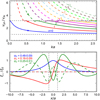Fig. 1. Transverse wave mode solutions for χ = 0.1. Top: dispersion plot, showing the solutions of Eq. (14) for χ = 0.1 as the normalised phase speed vph/vAi versus the normalised wave number ka, for the first eleven transverse harmonics. Solid (dashed) curves indicate trapped (leaky) modes. The normalised internal and external Alfvén speeds are indicated by dashed black lines. Bottom: normalised transverse displacement profile Pn(tanh(x/a)) sechα(x/a) as a function of x/a for three modes whose phase speed and wave number are indicated as coloured circles above. The solid (dashed) curves are the real (imaginary) part.

In order to characterise the transverse mode profile, the ODE (11) for the particular polynomial solution of wave number n is reformulated using the condition (13) as

$$\begin{array}{c}\hfill (1-{\tau }^2){\mathrm{P}}_n^{″}-2(\alpha +1)\tau {\mathrm{P}}_n^{\prime }+n(n+2{\alpha }_n+1){\mathrm{P}}_n=0.\end{array}$$(16)

For the case α_n = 0, Eq. (16) reverts to Legendre’s differential equation. However, in general we recognise Eq. (16) to be Gegenbauer’s differential equation:

$$\begin{array}{c}\hfill (1-{\tau }^2){\mathrm{C}}_n^{(\lambda {)}^{″}}-(2\lambda +1)\tau {\mathrm{C}}_n^{(\lambda {)}^{\prime }}+n(n+2\lambda ){\mathrm{C}}_n^{(\lambda )}=0,\end{array}$$(17)

with parameter $\lambda =\alpha +\frac{1}{2}>-\frac{1}{2}(\ne 0)$. We adopted the properties of this type of polynomial for our case (Abramowitz & Stegun 1965). The polynomial solution can be defined by the series

$$\begin{array}{c}\hfill {\mathrm{P}}_n(\tau ;\alpha )=C_n^{(\alpha +\frac{1}{2})}(\tau )={\displaystyle \sum _{l=0}^{\lfloor n/2\rfloor }\frac{{(-1)}^l\mathrm{\Gamma }(n-l+\alpha +\frac{1}{2})}{l!(n-2l)!\mathrm{\Gamma }(\alpha +\frac{1}{2})}{(2\tau )}^{n-2l},}\end{array}$$(18)

where Γ(z) is the Gamma function. The first few polynomials are P₀(τ; α) = 1 and P₁(τ; α) = (2α​ + ​1) τ. Further polynomials can be calculated using the recursive relation for fixed parameter α:

$$\begin{array}{c}\hfill n{\mathrm{P}}_n=(2n+2\alpha -1)\tau {\mathrm{P}}_{n-1}-(n+2\alpha -1){\mathrm{P}}_{n-2}.\end{array}$$(19)

For a fixed parameter α, polynomials of different orders are orthogonal:

$$\begin{array}{c}\hfill {\displaystyle \underset{-1}{\overset{+1}{\int }}{\mathrm{P}}_n(\tau ;\alpha ){\mathrm{P}}_m(\tau ;\alpha ){(1-{\tau }^2)}^{\alpha }\mathrm{d}\tau =N_n^2(\alpha ){\delta }_{\mathit{nm}},}\end{array}$$(20)

with

$$\begin{array}{c}\hfill N_n^2(\alpha )=\frac{\pi \mathrm{\Gamma }(n+2\alpha +1)}{2^{2\alpha }n!(n+\alpha +\frac{1}{2}){\mathrm{\Gamma }}^2(\alpha +\frac{1}{2})}.\end{array}$$(21)

For two polynomials with different parameters, the scalar product can be found as

$$\begin{array}{cc}\hfill N_{\mathit{nm}}^2(\alpha ,\beta )& ={\displaystyle \underset{-1}{\overset{+1}{\int }}{\mathrm{P}}_n(\tau ;\alpha ){\mathrm{P}}_m(\tau ;\beta ){(1-{\tau }^2)}^{\frac{\alpha +\beta }{2}}\mathrm{d}\tau }\hfill \\ \hfill & ={\displaystyle \sum _{l=0}^{\lfloor n/2\rfloor }\sum _{l^{\prime }=0}^{\lfloor m/2\rfloor }{a}_l^{(n)}{a}_{l^{\prime }}^{(m)}{I}_{\frac{n+m}{2}-l-l^{\prime },\frac{\alpha +\beta }{2}},}\hfill \end{array}$$(22)

with the integral

$$\begin{array}{c}\hfill I_{r,s}={\displaystyle \underset{-1}{\overset{+1}{\int }}}{\tau }^{2r}{(1-{\tau }^2)}^s\mathrm{d}\tau =\frac{1}{2}[1+{(-1)}^{2r}]\frac{\mathrm{\Gamma }[r+\frac{1}{2}]\mathrm{\Gamma }[s+1]}{\mathrm{\Gamma }[r+s+\frac{3}{2}]},\end{array}$$(23)

and coefficients

$$\begin{array}{c}\hfill a_l^{(n)}=\frac{{(-1)}^l{2}^{n-2l}\mathrm{\Gamma }(n-l+\alpha +\frac{1}{2})}{l!(n-2l)!\mathrm{\Gamma }(\alpha +\frac{1}{2})}.\end{array}$$(24)

This expression reverts to the standard orthogonality for equal parameters, that is, N_nm(α, α) = N_n(α) δ_nm. The Gegenbauer polynomials with fixed parameter α form a complete set so that any function, f(τ), can be expanded into them. Thus, we may expand the full solution for ${\widehat{\xi }}_{\perp }$ in x as

$$\begin{array}{c}\hfill {\widehat{\xi }}_{\perp }(x)={\displaystyle \sum _{n=0}^{\infty }{b}_n{\mathrm{P}}_n(tanh(x/a);{\alpha }_n){\mathrm{sech}}^{{\alpha }_n}(x/a),}\end{array}$$(25)

with weight coefficients

$$\begin{array}{c}\hfill b_n=\frac{1}{N_n^2({\alpha }_n)}{\displaystyle \underset{-1}{\overset{+1}{\int }}}{\widehat{\xi }}_{\perp }(\tau ){\mathrm{P}}_n(\tau ;{\alpha }_n){(1-{\tau }^2)}^{{\alpha }_n}\mathrm{d}\tau .\end{array}$$(26)

We explicitly write the parameter α_n with the index n as each harmonic will have a different value of α for a fixed value of k.

3.2. Effect of longitudinal structuring on the fast magnetoacoustic waves

To address the effect of stratification, we followed a methodology similar to that set out by Andries et al. (2005, 2009). We assumed that in the two-dimensional slab, the equilibrium density was also varying with y and so we may write the square of the Alfvén speed of the form $v_{\text{A}}^2(x,y)=v_{\text{A}}^2(x)G(y)$, where G(y) represents the longitudinal structuring. For our model, v_A(x) is given by Eq. (8) and G(y) = 1/F(y). The most straightforward manner to include this variation in the wave solution is to expand the transverse displacement into a Fourier series of sine functions:

$$\begin{array}{c}\hfill {\xi }_{\perp }=e^{-i\omega t}\sum _{m^{\prime }=1}^{\infty }{\widehat{\xi }}_{\perp ,m^{\prime }}(x)sin(k_{m^{\prime }}y),\end{array}$$(27)

with wave number k_m′ = m′π/L. Substituting this solution into Eq. (7) leads to the ODE:

$$\begin{array}{c}\hfill {\displaystyle \sum _{m^{\prime }=1}^{\infty }}G(y)sin(k_{m^{\prime }}y)\{v_A^2(x)[\frac{{\mathrm{d}}^2}{\mathrm{d}{x}^2}-k_m^{\prime 2}]+{\omega }^2\}{\widehat{\xi }}_{\perp ,n^{\prime }}=0.\end{array}$$(28)

We then project this equation onto the longitudinal state m by integrating this equation with the function sin(k_my) across the domain in y and with the normalisation factor 2/L. Thus, Eq. (28) reduces to

$$\begin{array}{c}\hfill {\displaystyle \sum _{m^{\prime }=1}^{\infty }{G}_{m{m}^{\prime }}{v}_A^2(x)[\frac{{\mathrm{d}}^2}{\mathrm{d}{x}^2}-k_m^{\prime 2}]{\widehat{\xi }}_{\perp ,m^{\prime }}=-{\omega }^2{\widehat{\xi }}_{\perp ,m},}\end{array}$$(29)

where

$$\begin{array}{c}\hfill G_{m{m}^{\prime }}=\frac{2}{L}{\displaystyle \underset{0}{\overset{L}{\int }}}G(y)sin(k_{m}y)sin(k_{m^{\prime }}y)\mathrm{d}y.\end{array}$$(30)

In a realistic loop atmosphere, the function G(y) is equal to one, except for narrow regions near the chromosphere where it drops to small values. Therefore, we expect G_mm′ to be close to δ_mm′. The small deviations from the delta function are the new physics being introduced. We then make use of the expansion for ${\widehat{\xi }}_{\perp ,m^{\prime }}(x)$ given by Eq. (25):

$$\begin{array}{c}\hfill {\widehat{\xi }}_{\perp ,m^{\prime }}(x)={\displaystyle \sum _{n^{\prime }=0}^{\infty }}{b}_{m^{\prime }{n}^{\prime }}{\mathrm{P}}_{n^{\prime }}(\tau ;{\alpha }_{m^{\prime }{n}^{\prime }}){(1-{\tau }^2)}^{\frac{{\alpha }_{m^{\prime }{n}^{\prime }}}{2}},\end{array}$$(31)

where ${\alpha }_{m^{\prime }{n}^{\prime }}=\sqrt{p}$ depends on k_m′ and ${\omega }_{m^{\prime }{n}^{\prime }}(k_{m^{\prime }}^{})$),  such that

$$\begin{array}{c}\hfill \{v_A^2(x)[\frac{{\mathrm{d}}^2}{\mathrm{d}{x}^2}-k_m^{\prime 2}]+{\omega }_{m^{\prime }{n}^{\prime }}^2\}{\mathrm{P}}_{n^{\prime }}(\tau ;{\alpha }_{m^{\prime }{n}^{\prime }}){(1-{\tau }^2)}^{\frac{{\alpha }_{m^{\prime }{n}^{\prime }}}{2}}=0.\end{array}$$(32)

Thus, Eq. (29) is reduced to

$$\begin{array}{cc}& {\displaystyle \sum _{m^{\prime }=1}^{\infty }\sum _{n^{\prime }=0}^{\infty }{b}_{m^{\prime }{n}^{\prime }}{G}_{m{m}^{\prime }}{\omega }_{m^{\prime }{n}^{\prime }}^2{\mathrm{P}}_{n^{\prime }}(\tau ;{\alpha }_{m^{\prime }{n}^{\prime }}){(1-{\tau }^2)}^{\frac{{\alpha }_{m^{\prime }{n}^{\prime }}}{2}}=}\hfill \\ \hfill & {\omega }^2{\displaystyle \sum _{n^{\prime }=0}^{\infty }{b}_{m{n}^{\prime }}{\mathrm{P}}_{n^{\prime }}(\tau ;{\alpha }_{m{n}^{\prime }}){(1-{\tau }^2)}^{\frac{{\alpha }_{m{n}^{\prime }}}{2}}.}\hfill \end{array}$$(33)

We project this equation onto the solution ${\mathrm{P}}_n(\tau ;{\alpha }_{\mathit{mn}}){(1-{\tau }^2)}^{\frac{{\alpha }_{\mathit{mn}}}{2}}$ and make use of expression (22) to find

$$\begin{array}{c}\hfill {\displaystyle \sum _{m^{\prime }=1}^{\infty }\sum _{n^{\prime }=0}^{\infty }(A_{mn{m}^{\prime }{n}^{\prime }}-{\omega }^2{B}_{mn{m}^{\prime }{n}^{\prime }})b_{m^{\prime }{n}^{\prime }}=0,}\end{array}$$(34)

with

$$\begin{array}{cc}& A_{mn{m}^{\prime }{n}^{\prime }}=G_{m{m}^{\prime }}{\omega }_{m^{\prime }{n}^{\prime }}^2{N}_{n{n}^{\prime }}^2({\alpha }_{\mathit{mn}},{\alpha }_{m^{\prime }{n}^{\prime }}),\hfill \end{array}$$(35)

$$\begin{array}{cc}\hfill & B_{mn{m}^{\prime }{n}^{\prime }}={\delta }_{m{m}^{\prime }}{N}_{n{n}^{\prime }}^2({\alpha }_{\mathit{mn}},{\alpha }_{m^{\prime }{n}^{\prime }}).\hfill \end{array}$$(36)

It should be noted that, if there is no longitudinal structuring, that is, G_mm′ = δ_mm′, then the eigenvalues ${\omega }^2={\omega }_{m^{\prime }{n}^{\prime }}^2$ of the individual modes naturally appear as solutions. Also, using the relation $\alpha =\sqrt{p}$, we would then see that $N_{n{n}^{\prime }}^2({\alpha }_{mn},{\alpha }_{m^{\prime }{n}^{\prime }})=N_{n^{\prime }}^2({\alpha }_{m{n}^{\prime }}){\delta }_{n{n}^{\prime }}$. Hence, the amplitudes would become trivially b_m′n′ = δ_mm′δ_nn′. The generalised eigenvalue problem is solved numerically by truncating the summations over m′ to M, and n′ to N − 1, and stacking indices as i = (m​ − ​1)N + n and j′=(m′​ − ​1)N + n′ so that the problem is reformulated as a traditional generalised eigenvalue problem:

$$\begin{array}{c}\hfill {\displaystyle \sum _{j=0}^{NM-1}(A_{\mathit{ij}}-{\omega }^2{B}_{\mathit{ij}})b_j=0.}\end{array}$$(37)

Figure 2 shows the structure and mode solution for the mode with the lowest frequency, for a particular equilibrium slab. We chose N = 10 and M = 20. This solution corresponds to the fundamental kink mode that is dominated by the mode (m = 1, n = 0). As expected, longitudinal structuring leads to coupling between modes with the same odd or even parity in m. Furthermore, there is coupling between modes of different transverse order, but that is less pronounced than the longitudinal mode coupling, In fact, in Fig. 2 there are more modes with degree n = 0 and higher values of wave number m, beyond the truncation, that have higher relative amplitudes than those shown in the figure with n > 0. The strength of the slope in the density profile controls the longitudinal mode coupling. The density contrast between the corona and the chromosphere controls the transverse mode coupling. Figure 3 shows the mode structure if the fundamental mode (m = 1, n = 0) has been removed. The higher longitudinal harmonics combine to build up the mode structure in the chromosphere and transition region. Importantly, the transverse spatial profile of these modes is narrower than the fundamental mode. The excitation of the slow waves through the coupling mechanism is proportional to the transverse derivative of this wave profile. The acoustic waves are primarily excited between the photosphere and the corona. Therefore, Fig. 3 shows that the transverse structuring of the acoustic waves is expected to have a narrower wave component superimposed on top of the fundamental one.

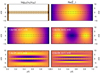Fig. 2. Structure of a given mode solution for the lowest frequency mode. Top left: relative Alfvén speed as a function of transverse and longitudinal coordinates, x and y, respectively, for the parameters values of χ = 0.1, ζ = 160, L = 252 Mm, a = 5 Mm, y0 = 6 Mm, and Δy = 1 Mm. The horizontal dashed lines indicate x = ±a. Top right: real part of the fundamental transverse eigenmode, ${\widehat{\xi }}_{\perp }$. The subsequent panels show some of the individual basic modes ${\widehat{\xi }}_{\perp ,m,n}$ that contribute to the full eigenmode. The relative amplitudes of those basic modes relative to ${\widehat{\xi }}_{\perp ,1,0}$ are given.

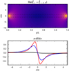Fig. 3. Transverse structuring of the fundamental transverse eigenmode. Top: real part of the fundamental transverse eigenmode as a function of transverse and longitudinal coordinates, x and y, respectively, from which the basic mode with longitudinal wave number m = 1 and transverse wave number n = 0 is subtracted, ${\widehat{\xi }}_{\perp }-{\widehat{\xi }}_{\perp ,1,0}$. The physical parameters are the same as for Fig. 2. Bottom: normalised transverse wave profile of the derivative of the fundamental transverse eigenmode, df/dx, as a function of x for three positions in y along the loop: 0 (red), y0 + Δy (blue), and L/2 (black).

Finally, for a general initial transverse displacement ξ_⊥, 0(x, y), we may write the further evolution as a superposition of the solutions as:

$$\begin{array}{c}\hfill {\xi }_{\perp }(x,y,t)={\displaystyle \sum _{j=0}^{NM-1}{c}_j{Q}_j(x,y)e^{-i{\omega }_{j}t},}\end{array}$$(38)

where

$$\begin{array}{c}\hfill Q_j(x,y)={\displaystyle \sum _{m=1}^M\sum _{n=0}^{N-1}{b}_{\mathit{mn}}^{(j)}sin(k_{m}y){\mathrm{P}}_n(\tau ;{\alpha }_{\mathit{mn}}){(1-t^2)}^{{\alpha }_{\mathit{mn}}},}\end{array}$$(39)

with coefficients

$$\begin{array}{c}\hfill c_j=\frac{\underset{0}{\overset{L}{\int }}\underset{-1}{\overset{+1}{\int }}{\xi }_{\perp ,0}{Q}_j\mathrm{d}\tau \mathrm{d}y}{\frac{L}{2}\sum _{m=1}^M\sum _{n=0}^{N-1}{(b_{\mathit{mn}}^{(j)})}^2{N}_n^2({\alpha }_{\mathit{mn}})}.\end{array}$$(40)

The analysis of the wave mode presented refers to fast magnetoacoustic oscillations only because in the zero plasma-β limit, the slow magnetoacoustic oscillations are absent. However, with a finite plasma-β, as is the case in the simulations presented later in the paper, slow oscillations are also present. With longitudinal structuring, such as defined by Eq. (2), it may be possible to have an additional hybrid transverse oscillation, with a similar frequency as the basic fast mode, which has a fast magnetoacoustic wave number in the corona but a slow magnetoacoustic wave number in the chromosphere. To include a finite plasma-β in the analytical wave modelling, the transverse Epstein density profile has to be replaced with, for example, a piece-wise uniform density profile in the transverse direction and the full fourth order magnetoacoustic wave equation has to be solved as an initial value problem. This is out of the scope of the paper, but we highlight in the simulations where the presence of slow magnetoacoustic transverse oscillations has an effect on the results presented.

3.3. Acoustic coupling in a one-dimensional model with longitudinal structuring

The basic model that describes the linear coupling between the transverse loop oscillation and acoustic waves through a reflective hard boundary has been given in Terradas et al. (2011) and White & Verwichte (2021). To model this coupling analytically in a finite-width transition region, we introduced simplifications from the two-dimensional slab model to keep the problem analytically tractable. First, we did not consider transverse structuring, such that x became an ignorable coordinate. This is reasonable as we expect the acoustic wave solution in two dimensions to still be proportional to the derivative of the transverse wave profile. Secondly, we solved for normal modes instead of an initial-value problem. Thirdly, we focused on the coupling at only one footpoint, in the knowledge that the behaviour is exactly the same at the other footpoint, except mirrored in the x-direction. Finally, we simplified the density structure to be piece-wise continuous with a linear density profile between a uniform chromosphere and corona:

$$\begin{array}{c}\hfill \frac{{\rho }_0(y)}{{\rho }_{\mathrm{c}}}=\{\begin{array}{cc}\zeta \hfill & 0\le y<y_0-\frac{\mathrm{\Delta }y}{2}\hfill \\ \frac{1}{2}(1+\zeta )+(1-\zeta )\left(\frac{y-y_0}{\mathrm{\Delta }y}\right)\hfill & |y-y_0|\le \frac{\mathrm{\Delta }y}{2}\hfill \\ 1\hfill & y>y_0+\frac{\mathrm{\Delta }y}{2}\hfill \end{array},\end{array}$$(41)

with ζ = ρ_ch/ρ_c being the density contrast of the chromosphere relative to the corona. The equilibrium magnetic field and plasma pressure were uniform throughout the domain. Hence, the plasma-β remained constant. We introduced the constant quantity $\stackrel{\sim }{\beta }={c_{\text{S}}}^2/{{\mathit{v}}_{\text{A}}}^2$. We employed the same methodology as used in White & Verwichte (2021) to consider finite plasma-β effects as a perturbation. Thus, to first approximation, the transverse wave is solved in the zero plasma-β limit. Thus, the transverse displacement, ${\xi }_{\perp }={\widehat{\xi }}_{\perp }(\mathit{y})exp[i(k_{\perp }x-\omega t)]$, satisfies the ODE

$$\begin{array}{c}\hfill \frac{{\mathrm{d}}^2{\widehat{\xi }}_{\perp }}{\mathrm{d}{y}^2}+{\kappa }^2(y){\widehat{\xi }}_{\perp }=0,\end{array}$$(42)

with longitudinal wave number, κ(y), defined as

$$\begin{array}{c}\hfill {\kappa }^2(y)=\frac{{\omega }^2}{v_{\mathrm{Ac}}^2}\frac{{\rho }_0(y)}{{\rho }_{\mathrm{c}}}-k_{\perp }^2.\end{array}$$(43)

The solution that satisfies the boundary condition ${\widehat{\xi }}_{\perp }(0)=0$ is

$$\begin{array}{c}\hfill {\widehat{\xi }}_{\perp }(y)=\{\begin{array}{cc}{D}_{0}sin({\kappa }_{\mathrm{ch}}y)\hfill & y<y_0-\frac{\mathrm{\Delta }y}{2}\hfill \\ C_{\mathrm{T}}\mathrm{Ai}(s)+D_{\mathrm{T}}\mathrm{Bi}(s)\hfill & |y-y_0|\le \frac{\mathrm{\Delta }y}{2}\hfill \\ C_{1}sin({\kappa }_{\mathrm{c}}y)+D_{1}cos({\kappa }_{\mathrm{c}}y)\hfill & y>y_0+\frac{\mathrm{\Delta }y}{2}\hfill \end{array},\end{array}$$(44)

where D₀, C_T, D_T, C₁, and C₂ are integration constants, which are solved in favour of the displacement amplitude at the loop top, ξ₀, using continuity of displacement and magnetic pressure at y = y₀​ ± ​Δy/2. κ_ch and κ_c are the longitudinal wave numbers in the chromosphere and corona, respectively. The functions Ai(s) and Bi(s) are Airy functions of the first and second kind, respectively, as a function of the coordinate

$$\begin{array}{c}\hfill s(y)=-{\alpha }^{1/3}{\kappa }^2(y),\end{array}$$(45)

with

$$\begin{array}{c}\hfill \alpha ={\left(\frac{v_{\mathrm{Ac}}^2\mathrm{\Delta }y}{{\omega }^2(\zeta -1)}\right)}^2.\end{array}$$(46)

The slow magnetoacoustic wave driven by the transverse oscillation is characterised by the longitudinal displacement, ${\xi }_{\Vert }={\widehat{\xi }}_{\Vert }(\mathit{y})exp[i(k_{\perp }x-\omega t)]$, and obeys the ODE

$$\begin{array}{c}\hfill [\frac{{\mathrm{d}}^2}{\mathrm{d}{y}^2}+K^2(y)]{\widehat{\xi }}_{\Vert }=-i{k}_{\perp }\frac{\mathrm{d}{\widehat{\xi }}_{\perp }}{\mathrm{d}y},\end{array}$$(47)

with

$$\begin{array}{c}\hfill K^2(y)=\frac{{\omega }^2}{c_{\mathrm{S}}^2(y)}=\frac{1}{\stackrel{\sim }{\beta }}({\kappa }^2(y)+k_{\perp }^2).\end{array}$$(48)

The solution in the chromosphere that satisfies the boundary condition ${\widehat{\xi }}_{\Vert }(0)=0$ and allows for only a slow wave in the corona that propagates away from the transition region, is written as

$$\begin{array}{c}\hfill {\widehat{\xi }}_{\Vert }(y)=\{\begin{array}{cc}{\mathcal{D}}_{0}sin(K_{\mathrm{ch}}y)+\mathbb{F}(y)\hfill & y<y_0-\frac{\mathrm{\Delta }y}{2}\hfill \\ {\mathcal{C}}_{\mathrm{T}}\mathrm{Ai}(z)+{\mathcal{D}}_{\mathrm{T}}\mathrm{Bi}(z)+\mathbb{G}(y)\hfill & |y-y_0|\le \frac{\mathrm{\Delta }y}{2}\hfill \\ {\mathcal{C}}_1{e}^{i{K}_{\mathrm{c}}y}+\mathbb{H}(y)\hfill & y>y_0+\frac{\mathrm{\Delta }y}{2}\hfill \end{array},\end{array}$$(49)

where 𝒟₀, 𝒞_T, 𝒟_T, and 𝒞₁ are integration constants that are written through continuity of displacement and pressure at y = y₀​ ± ​Δy/2 in terms of the transverse displacement amplitude, ξ₀. The coordinate z is defined as

$$\begin{array}{c}\hfill z(y)=-{\stackrel{\sim }{\beta }}^{2/3}{\alpha }^{1/3}{K}^2(y).\end{array}$$(50)

We note that

$$\begin{array}{c}\hfill s={\stackrel{\sim }{\beta }}^{1/3}z+{\alpha }^{1/3}{k}_{\perp }^2.\end{array}$$(51)

The particular solution is defined using the functions:

$$\begin{array}{cc}& \mathbb{F}(y)=\frac{i{k}_{\perp }{\kappa }_{\mathrm{ch}}{D}_0}{K_{\mathrm{ch}}^2-{\kappa }_{\mathrm{ch}}^2}[cos(K_{\mathrm{ch}}y)-cos({\kappa }_{\mathrm{ch}}y)],\hfill \end{array}$$(52)

$$\begin{array}{cc}& \mathbb{G}(y)=\mathrm{Ai}(z){\displaystyle \underset{0}{\overset{z}{\int }}f(z\prime )\mathrm{Bi}(z\prime )\mathrm{d}z\prime -\mathrm{Bi}(z)\underset{0}{\overset{z}{\int }}f(z\prime )\mathrm{Ai}(z\prime )\mathrm{d}z\prime ,}\hfill \end{array}$$(53)

$$\begin{array}{cc}& \mathbb{H}(y)=\frac{i{k}_{\perp }{\kappa }_{\mathrm{c}}}{K_{\mathrm{c}}^2-{\kappa }_{\mathrm{c}}^2}[C_{1}sin({\kappa }_{\mathrm{c}}y)-D_{1}cos({\kappa }_{\mathrm{c}}y)],\hfill \end{array}$$(54)

with

$$\begin{array}{c}\hfill f(z)=i\pi k_{\perp }{\stackrel{\sim }{\beta }}^{2/3}{\alpha }^{1/6}[C_{\mathrm{T}}\mathrm{Ai}\prime (s)+D_{\mathrm{T}}\mathrm{Bi}\prime (s)].\end{array}$$(55)

Figure 4 shows the spatial dependence of key physical variables. The Alfvén and sound speeds are lower in the chromosphere. Therefore, the profiles for both transverse and acoustic wave solutions with a fixed period of oscillation have shorter length scales there compared within the corona. The coupling term, namely the driving term in the acoustic wave equation, has a clear dependence on y. At every location acoustic waves are excited by the coupling term and are launched to travel in both directions, but are in anti-phase in displacement. If locally, the driving is equal, then those waves are cancelled out. However, where the coupling term varies spatially, there is an asymmetry in wave generation so that a finite flux of acoustic waves is excited. Figure 4 shows these locations to be in the transition region and, specifically for this choice of geometry, near the top of the transition region. From there, acoustic waves propagate directly upwards into the corona, but also downwards into the chromosphere. They reflect at the photospheric boundary, with a phase-shift of π, and travel back upwards. At that boundary, the coupling term is also finite as the derivative, ∂ξ_⊥/∂y, jumps from a finite value to zero. Hence, acoustic waves travel from the lower boundary upwards through the chromosphere into the transition region. The various acoustic waves interfere and, depending on acoustic travel times, this is either constructive or destructive. We define the acoustic travel time from the photosphere to the top of the transition region as

$$\begin{array}{c}\hfill {\tau }_{\mathrm{S},\mathrm{ch}}={\displaystyle \underset{0}{\overset{y_0+\mathrm{\Delta }y}{\int }}\frac{\mathrm{d}y}{c_{\mathrm{S}}(y)}.}\end{array}$$(56)

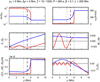Fig. 4. Spatial profiles across the transition region of the equilibrium mass density, ρ0(y)/ρ0c, Alfvén speed, vA(y), transverse displacement, ξ⊥/ξ0, derivative of the transverse displacement, ∂/∂y(ξ⊥/ξ0), the acoustic coupling term, $c_{\text{S}}{}^2(y)k_{\perp }\partial /\partial y\left({\xi }_{\perp }/{\xi }_0\right)$, and the longitudinal displacement, ξ∥/ξ0. The vertical dashed and dotted lines indicate the positions y0 and y0 ± Δy, respectively. The blue and red curves are the wave solutions for a density contrast ζ = 10 and 1000, respectively.

Figure 5 shows the relative amplitude of the acoustic wave propagating from the transition region into the corona as a function of the transition region width and contrast. It shows that, overall, the rate of acoustic wave generation matches the one without a transition region and a fully reflective boundary (White & Verwichte 2021). There are important departures at key parameter values corresponding to multiples of 4τ_S, ch. For τ_S, ch/P = 0.25, 0.75, 1.25,... the wave launched downwards from the transition region reflects at the photosphere and reaches the corona approximately in anti-phase with the directly excited acoustic wave there. The acoustic wave excited at the photosphere directly is shifted in phase by ±π/2. The net result is destructive interference and less acoustic wave power is launched into the corona. For τ_S, ch/P = 0.5, 1.5, 2.5, ... the reflected wave and direct wave from the transition region are in phase. The photospherically launched wave is in anti-phase. Overall, the acoustic wave power is the same as in the case without a transition region, that is, using Eq. (24) from White & Verwichte (2021). For an integer value of τ_S, ch/P, all waves are in phase when they reach the corona, resulting in a net constructive interference and an enhancement in acoustic power. The location of peaks and dips do not exactly match the multiples of the acoustic travel time because the wave excitation does not occur at a single position, but rather over a finite extent in and around the transition region, which is more apparent when the density contrast is modest.

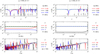Fig. 5. Displacement amplitudes of the acoustic wave propagating from the transition region into the corona, |𝒞1|, relative to the transverse loop displacement at the loop top, ξ0. Top panels: relative amplitude as a function of density contrast, ζ, for three values of transition region width, Δy, at a fixed period, P. Middle panels: relative amplitude as a function of Δy for three values of ζ at a fixed P. Bottom panels: relative amplitude as a function of P for three values of ζ at fixed Δy. The green dashed line shows the relative amplitude obtained from Eq. (24) from White & Verwichte (2021) for a fully reflective boundary. Vertical dashed and dotted lines represent values where the travel time from the lower boundary to y0 are multiples of 4τS, ch/P, for the parameters of the black curve. The left and right sets of panels are for y0 = 5 Mm and y0 = 2Mm, respectively. Also, $\stackrel{\sim }{\beta }=0.083$, which corresponds to a plasma-β = 0.1.

4. Numerical modelling

Simulations were performed using Lare2d, a Lagrangian remap code that solves the MHD equations in two dimensions (Arber et al. 2001), where we assumed a fully ionised, conductive plasma. An average particle mass of $\overline{m}=0.6m_{\mathrm{p}}$ was chosen, where m_p is the proton mass. This represents the average particle mass for the corona, which is the bulk of the computational domain. In reality, the chromosphere will have a higher value of $\overline{m}$. We chose a coronal loop of length L = 252 Mm with a magnetic field in the y-direction and with magnitude B₀ = 2.7 × 10⁻³ T on the loop axis. The temperature at the top of the loop was chosen to be 1 MK. The mass density at the loop top followed from the plasma-β = 0.085 as ρ_c = 1.8 × 10⁻¹¹ kgm⁻³. The density profile as a function of x and y is given by Eq. (1). To ensure an adequate resolution of the transition region and chromosphere, without the need for an excessive simulation runtime, we set the position of the transition region to be y₀ = 6 Mm. The mass density contrast between the chromosphere and corona, ζ, and the width of the transition region, Δy, were allowed to vary between simulation runs. Both the temperature and density profiles along the loop are shown in Fig. 6. In the transverse x-direction, the numerical domain spanned −10L ≤ x ≤ 10L. This ensured that the trapped transverse wave profile decayed to a sufficiently small value and prevented any wave reflection at the boundaries from interfering with our analyses. The simulations were run with a numerical grid of 32 000 × 1600.

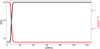Fig. 6. Equilibrium temperature and density profiles along the loop at x = x0, which are represented by the solid black and red lines, respectively. The dashed line indicates the positions at a distance y0 from the photosphere.

The study was limited to loops with an isothermal transverse profile. This removed the effect of phase mixing due to changes in sound speed across the loop (Voitenko et al. 2005), so that we could focus on the effect of the transition region on wave coupling. Across the loop, the mass density varied as given by Eq. (2) with a contrast and loop half-width of ξ = 0.1 and a = 0.05L, respectively. The magnetic field varied with x according to Eq. (4) to ensure pressure balance across the loop. All simulations were initialised with a transverse velocity perturbation of the form

$$\begin{array}{c}\hfill v_{x,0}(x,y)=v_{0}f(x)sin{k}_{\Vert }y,\end{array}$$(57)

where v₀ is the velocity amplitude, f(x) is the transverse velocity profile and k_∥ = π/L is the longitudinal wave number of the fundamental standing wave, corresponding to an excitation along the whole loop. Simulations were also performed with a velocity profile that had a non-zero, sinusoidal profile only in the corona. Because the results are not significantly different, these simulations are not shown here. We used an initial perturbation that matched the fundamental kink mode for a uniform slab (n = 0) from Eq. (25) to excite, as closely as possible, the fundamental kink mode in the numerical domain, even in the presence of a transition region and finite β, in order to reduce initial transients. However, as we shall see, this cannot prevent the excitation of other temporal modes, especially in the chromosphere.

4.1. Transverse loop oscillations

To begin the analysis of wave coupling, we considered a loop with a density contrast between a chromosphere and corona of ζ = 160 and a transition region width of Δy = 1.0 Mm. Using Eq. (4), this corresponds to a chromospheric temperature of 6250 K. The initial perturbation has a velocity amplitude v₀ = 0.001v_Ai, where ${\mathit{v}}_{\mathrm{Ai}}=B(0)/\sqrt{\mu {\rho }_{\mathrm{c}}}$ is the Alfvén velocity on the loop axis. With such small perturbations, the simulation remains essentially linear. The longitudinal and perpendicular velocity components basically coincide with the y and x components of the velocity in the simulations. The time evolution of the standing kink oscillation is shown in Fig. 7, where we defined the Alfvén travel time along the loop twice as

$$\begin{array}{c}\hfill {\tau }_{\mathrm{A}}=2{\displaystyle {\int }_0^{\mathrm{L}}\frac{\mathrm{d}y}{v_{\mathrm{Ai}}\left(y\right)}.}\end{array}$$(58)

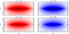Fig. 7. Temporal evolution of the transverse oscillation for a simulation with plasma-β = 0.08 and an initial perturbation v0 = 0.001vAi. The thick dashed lines indicate the positions of the transition region at y0 from the photosphere. The thin dashed lines are at x = ±a Mm from the loop axis.

This travel time is longer than the period of the fundamental standing mode due to its two-dimensional nature and because it is governed more closely by the external Alfvén speed. Along with the expected fundamental standing oscillation in the corona, we observe the development of an additional higher spatial harmonic at the loop footpoints. These harmonics are out of phase with the fundamental oscillation, and resemble the n = 0, m = 3 mode, as expected from the analytical description of Sect. 3, and as clearly seen in Fig. 3.

The transverse velocity was decomposed into Fourier sine series, as was done analytically in Sect. 3 (see Eq. (27)). This allowed us to determine the contribution of different longitudinal wave numbers k_m to the transverse velocity. We did not decompose the velocity into its transverse wave modes with wave numbers n, as this is more difficult to achieve. After subtracting the mode with m = 1, and for all n, v_⊥, 1, from the perpendicular velocity, we were left with the contribution from the higher longitudinal harmonics. The result is shown in Fig. 8. As expected, the higher longitudinal modes build up in the transition region and the chromosphere, closely resembling the mode structure obtained analytically shown in Fig. 3. These higher harmonics have a narrower transverse spatial profile than the fundamental mode. Alongside this, in Fig. 3, we plot the transverse derivative of the full transverse velocity. As this derivative appears as a factor in the slow mode driving term, it describes the transverse shape of the resulting slow modes. The derivative emphasises again that the transverse structure is narrower around the transition region and the chromosphere compared with at the loop top, and narrower compared to a purely fundamental m = 1 mode (White & Verwichte 2021). This region is also where we expect the slow mode coupling to be the strongest. This finding is in line with the analytical analysis. We speculate that this is due to the presence of higher temporal harmonics in the simulations, that is to say, modes with odd m ≥ 3, n = 0 spatial harmonics. But also, in a finite plasma-β, a transverse magnetoacoustic mode may appear with characteristics of a slow magnetoacoustic wave in the lower atmosphere that has a similar frequency to the basic fast transverse oscillation.

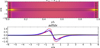Fig. 8. Transverse structuring of the transverse velocity. Top: remainder of the perpendicular velocity, vx, with all modes with longitudinal wave number m = 1 subtracted, at time t/τA = 0.66. The lines are the same as those explained in Fig. 7. Bottom: profiles of the derivative of the transverse velocity in the x-direction, ∂vx/∂x, at three positions along the loop: y = 0 (red), y = y0 + δy (blue), and y = L/2 (black), and at two times: t/τA = 0.66 (solid lines) and t/τA = 0.93 (dashed lines).

4.2. Acoustic coupling due to longitudinal structuring

A useful quantity to assess the wave coupling is afforded by the term $c_{\text{S}}{}^2{\partial }^2\xi /\partial x\partial y$ in Eq. (5), which is the driving term for the slow waves (Terradas et al. 2011; White & Verwichte 2021). In Figs. 9 and 10, we focus on a simulation with a plasma-β = 0.08, and an initial perturbation v₀ = 0.001v_Ai. Figure 9 shows the analogous coupling term ${c_{\text{S}}}^2{\partial }^2{\mathit{v}}_x/\partial x\partial \mathit{y}$ alongside the parallel velocity, v_y. We see that the coupling term is almost entirely concentrated around the beginning of the transition region, with a maximum at a distance of approximately 10 Mm along the loop, and it falls off sharply further down towards the chromosphere. The coupling is also concentrated within the loop and is, as expected, anti-symmetric about the loop axis and about the centre of the loop.

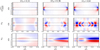Fig. 9. Evolution of the acoustic coupling. Top: temporal evolution of the coupling term $c_{\text{S}}{}^2{\partial }^2{v}_x/\partial x\partial y$ across the entire loop. Middle: temporal evolution of the longitudinal velocity, vy. Bottom: temporal evolution of vy in a restricted domain near the left footpoint. The dashed line indicates the position of the transition region at y = y0, and the dotted-dashed line indicates the distance y0 ± Δy.

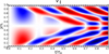Fig. 10. Longitudinal velocity, vy, along the loop averaged over the domain where x ≥ 0. Lines indicate the centre of the transition region y0.

Alongside this coupling term, we observe the generation of longitudinal waves into the corona from the transition region, where the coupling is largest. This confirms the simulation result found by Terradas et al. (2011) for the generation of slow waves in the presence of a sharp transition region in density, but in a transversely unstructured plasma. The location of the slow wave generation is clearly visible in a distance-time plot of the longitudinal velocity, seen as propagating waves from the footpoints towards the loop top in Fig. 10. As was found in the previous study without a transition region (White & Verwichte 2021), the longitudinal field is found to be anti-symmetric about the loop axis and the centre of the loop. This symmetry will have consequences for the detectability of the slow waves as the exact orientation of the observer with respect to the loop is important. These waves are found to be more concentrated about the loop axis relative to longitudinal waves in a loop with no transition region. We also observe the generation of shorter wavelength slow waves that travel from the bottom of the transition region down into the chromosphere, as well as waves propagating upwards from the chromosphere. The difference in wavelength is understood from the difference in temperature between the chromosphere and the corona, that is, ${\lambda }_{\mathrm{S},\mathrm{ch}}=\sqrt{T_{\mathrm{ch}}/T_{\mathrm{c}}}{\lambda }_{\mathrm{S},\mathrm{c}}$, where the subscripts ‘c’ and ‘ch’ indicate ‘coronal’ and ‘chromospheric’, respectively. At the site of excitation in the transition region, the upward and downward propagating slow waves are in anti-phase with respect to each other.

To better understand the generation of these slow waves, we examined the sound power flux, S = p v_y, which is the product of plasma pressure and longitudinal velocity. This quantity describes the energy flux of the slow waves per unit time and highlights the propagation direction of slow wave power. The average sound power across the whole transverse direction is shown in Fig. 11. From the top panel, we can clearly see the propagation of slow waves from the transition region to the loop top where the waves begin to interfere. In the bottom panel, we focus on one of the loop footpoints. We observe the generation of waves with differing properties. Alongside the upward propagating slow waves, we observe downward propagating waves from the transition region, which reflect at the lower boundary of the photosphere and are out of phase with the large wavelength, upward propagating waves. Additionally, there is the generation of upward propagating waves from the lower boundary due to the hard boundary conditions there, which interfere with the downward propagating waves from the transition region. We superimposed sounds rays in Fig. 11 to highlight the pattern of the various wave propagations. These initial-value simulations show the same type of wave propagatory behaviour as shown in the analytical normal mode analysis in Sect. 3.3. In the simulations, the acoustic travel time in the lower atmosphere is τ_S, ch = 480 s and the period is P = 360 s. Hence, τ_S, ch/P = 4/3, which lies between the value of 5/4 where the upward propagating slow waves that are excited in the transition region encounter destructive interference from slow waves propagating upwards from the chromosphere (those excited and reflected at the photosphere) and the value of 3/2 where the direct and reflected upward propagating slow waves interfere constructively. Therefore, the various slow waves are not in resonance. This can be seen in Fig. 11, where the amplitude of the slows waves in the corona modulates over time due to the interference from the slow waves propagating upwards from the chromosphere, but does not increase monotonically.

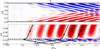Fig. 11. Sound power averaged across the entire loop. Lines indicate the same positions as explained in Fig. 9. Top: sound power along the entire loop. Bottom: sound power near the loop footpoint. The solid lines indicate slow wave rays from upward and downward propagating waves from the transition region as well as upward propagating waves from the photospheric boundary.

4.3. Wave energetics

We examined the kinetic energy in the corona and in the lower atmosphere below the upper transition region. We split the kinetic energy at any time into perpendicular and parallel parts, and normalised these with respect to the initial kinetic energy due to the initial transverse perturbation:

$$\begin{array}{cc}\hfill {\left(\frac{{\mathrm{kE}}_{\perp }}{{\mathrm{kE}}_{\perp ,0}}\right)}_{\mathrm{c}}& =\frac{1}{2{\mathrm{kE}}_{\perp ,0}}{\displaystyle \underset{y_0+\mathrm{\Delta }y}{\overset{L-y_0-\mathrm{\Delta }y}{\int }}\underset{-\infty }{\overset{+\infty }{\int }}\rho v_x^2\mathrm{d}x\mathrm{d}y,}\hfill \end{array}$$(59)

$$\begin{array}{cc}\hfill {\left(\frac{{\mathrm{kE}}_{\Vert }}{{\mathrm{kE}}_{\perp ,0}}\right)}_{\mathrm{c}}& =\frac{1}{2{\mathrm{kE}}_{\perp ,0}}{\displaystyle \underset{y_0+\mathrm{\Delta }y}{\overset{L-y_0-\mathrm{\Delta }y}{\int }}\underset{-\infty }{\overset{+\infty }{\int }}\rho v_y^2\mathrm{d}x\mathrm{d}y,}\hfill \end{array}$$(60)

$$\begin{array}{cc}\hfill {\left(\frac{{\mathrm{kE}}_{\perp }}{{\mathrm{kE}}_{\perp ,0}}\right)}_{\mathrm{ch}}& =\frac{1}{{\mathrm{kE}}_{\perp ,0}}{\displaystyle \underset{0}{\overset{y_0+\mathrm{\Delta }y}{\int }}\underset{-\infty }{\overset{+\infty }{\int }}\rho v_x^2\mathrm{d}x\mathrm{d}y,}\hfill \end{array}$$(61)

$$\begin{array}{cc}\hfill {\left(\frac{{\mathrm{kE}}_{\Vert }}{{\mathrm{kE}}_{\perp ,0}}\right)}_{\mathrm{ch}}& =\frac{1}{{\mathrm{kE}}_{\perp ,0}}{\displaystyle \underset{0}{\overset{y_0+\mathrm{\Delta }y}{\int }}\underset{-\infty }{\overset{+\infty }{\int }}\rho v_y^2\mathrm{d}x\mathrm{d}y,}\hfill \end{array}$$(62)

$$\begin{array}{cc}\hfill {\mathrm{kE}}_{\perp ,0}& =\frac{1}{2}{\displaystyle \underset{0}{\overset{L}{\int }}\underset{-\infty }{\overset{+\infty }{\int }}{\rho }_0{v}_{x,0}^2\mathrm{d}x\mathrm{d}y.}\hfill \end{array}$$(63)

The kinetic energies oscillate with the wave period as there is energy partition with magnetic energy, and to a lesser extent internal energy, for the transverse oscillation, and with internal energy for the slow wave. We examined the exchange of energy between the transverse and slow waves, and between the corona and the lower atmosphere, over longer timescales.

Figure 12 shows that the vast majority of the initial energy perturbation is to be found within the corona, in the form of a perpendicular kinetic energy component, with only a few percent of the initial energy perturbation in the transition region. Observing the trend in kE_⊥ from maxima to maxima, we observe a consistent transfer of kinetic energy from the corona into the transition region. This energy transfer continues until almost half of the total energy is located within the transition region, after which the process reverses and energy is transferred back into the corona. The beat has a period of 1.8τ_A. This value changes with the plasma-β. This suggests that the beat occurs due to the excitation of an additional hybrid slow magnetoacoustic oscillation with a similar frequency and longitudinal profile as the basic fast mode in the corona, but a shorter wavelength in the chromosphere determined by the sound speed. This process would show as a modulation of the amplitude of the transverse loop oscillation at the loop top with a drop in amplitude of about 70%. However, we can imagine a process in which the damping of the waves entering the transition region and chromosphere would lead to an irreversible loss of energy in the corona, and hence damping of the transverse waves within a few periods (De Pontieu et al. 2001). This process would be in addition to the leading damping mechanism of resonant absorption. It is clear that this process is governed by the presence of these two modes with close frequencies. More work is required, with more realistic lower atmospheric-density and temperature profiles, as well as dissipation that is afforded, for example, by ion-neutral reactions, to confirm the importance of this process.

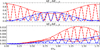Fig. 12. Evolution of the kinetic energy of the system. Top: normalised perpendicular component of the kinetic energy, kE⊥/kE⊥, 0. The dashed red and blue lines represent the energy within the corona and the lower atmosphere, respectively. The solid lines are envelopes. Bottom: normalised parallel component of the kinetic energy, kE∥/kE⊥, 0. The dashed red and blue lines represent the energy within the corona and the lower atmosphere, respectively. The solid lines are envelopes.

The bottom panel in Fig. 12 shows the parallel kinetic energy component that correlates to the propagating slow wave energy. There is an increase in slow wave energy in both the corona and the transition region due to the constant sources of wave coupling at the transition region and the photosphere. At a later time, we observe a decrease in the coronal energy, and given that this time is approximately equal to the travel time from one side of the corona to the other, the energy loss is explained by these waves entering into the opposite transition region. This is confirmed by the simultaneous increase in the gradient of the transition region energy. The loss of energy in the transition region due to lateral wave leakage is negligible compared with the sources of wave energy.

4.4. Analysis of the slow wave density perturbations

We studied the effect of the transition region parameters Δy and β, which describe the width of the transition region and the density contrast between the corona and the chromosphere, respectively, on the resulting propagating slow wave density perturbation. This allowed us to determine the maximum theoretical density perturbation and the behaviour as we moved towards more realistic chromospheric conditions. As before, we took a loop of length L = 252Mm, a plasma-β = 0.08, and a purely linear velocity perturbation of v₀ = 0.001v_Ai. The effect of the plasma-β on the generation of slow waves has been studied in Terradas et al. (2011) and White & Verwichte (2021). To distinguish the slow modes from the density perturbation due to the standing fast mode, we applied a high band pass filter on the y-coordinate to remove the low-wavelength standing fast mode in the corona with a wave number k_f = π/L, given the slow mode wavelength was ${\lambda }_s\simeq \frac{c_s}{{\mathit{v}}_A}{\lambda }_f$.

The left panel of Fig. 13 shows the dependence of the maximum slow mode density perturbation in the corona on the density contrast between the chromosphere and the corona ζ. We observe that the amplitude of the slow mode density perturbation increases by an order of magnitude over the range of ζ. This increase is most rapid for 80 ≥ ζ ≤ 100, with a smaller gradient around this value. We also find that for decreasing δy, we obtain an increase in density perturbation, which corresponds to an increase in the gradient of the density. The right panel of Fig. 13 shows the slow mode perturbation dependence on the density gradient at y = y₀. For fixed ζ, an increase in gradient may be seen as a decrease in the transition region width, Δy. The density perturbation increases with an increasing gradient, although its dependence on the gradient is weaker than on ζ. The density amplitude increase slows down for larger values of ζ. It is unclear whether it asymptotically tends to a maximum value or reaches a maximum at a fixed value of ζ. Realistically, the transition region has a value of ζ of at least 1000. We did not extend the parameter study to such large values due to computational constraints on the grid size and the physicality of the used density and temperature profiles. For the range of values of ζ in Fig. 13, the ratio τ_S, ch/P varies from 0.71 for ζ = 40 to 1.36 for ζ = 160. In the analytical modelling in Sect. 3.3, the slow waves were predicted to have a resonance at τ_S, ch/P = 1, as well as destructive interference at τ_S, ch/P = 0.75 and 1.25. This is not visible in the numerical result. Importantly, a direct comparison is not possible as the analytical modelling relies on normal mode analysis, whilst the numerical results are taken at a finite time when mode resonances will not have had sufficient time to build up. However, we note that the resonance τ_S, ch/P = 1 falls between ζ = 80 and ζ = 100, where the numerical amplitude profile has its maximum gradient.

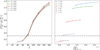Fig. 13. Relative maximum slow mode density perturbation in the corona. We divided this by $\sqrt{\beta }{\mathit{v}}_0/{\mathit{v}}_{\mathrm{Ai}}$ to allow this plot to be used as a reference. Left: as a function of the density contrast between the chromosphere and the corona for different transition region widths, Δy. Right: as a function of the density gradient at y = y0 and the corona for different transition region widths, Δy. The horizontal dashed-dotted lines give the value of the perturbation for a loop with no atmosphere. Connecting lines have been included to both plots as visual aids.

5. Application to observations

Terradas et al. (2011) suggested that intensity perturbations observed by Verwichte et al. (2010) in a loop with transverse oscillation may be explained via the linear wave coupling due to line-tying conditions at the loop footpoints. Variations in the intensity accompanying the transverse loop oscillations with the same period were observed by TRACE and EIT/SoHo. These observations were simulated by White & Verwichte (2021), given loop parameters that closely resembled one of the loops observed by Verwichte et al. (2010). In this model, the loop had no longitudinal structuring, with the coupling caused by the hard boundary conditions at the loop footpoint. White & Verwichte (2021) predicted a maximum intensity oscillation due to the slow mode of order 4.5%, which is smaller than the maximum amplitude 15% observed by Verwichte et al. (2010). In both works, there was a longer timescale oscillation of 80 min, which is explained by the ponderomotive force, which is a major factor for oscillations greater than 10% of the Alfvén speed. In White & Verwichte (2021), this force dominates the intensity perturbation, although it is masked by the outflows associated with the coronal mass ejection that triggered the transverse oscillations reported by Verwichte et al. (2010).

We return to this simulation but now include a longitudinally structured loop. Our equilibrium values were chosen to resemble those of the loop studied by Verwichte et al. (2010). Although the phase velocity more closely matches the external Alfvén speed instead of the kink speed for slab geometry, our equilibrium values differed slightly in order to obtain the observed oscillation period. We took a loop of length L = 702 Mm, the transition region position y₀ = 6 Mm, the transition region width Δy = 1 Mm, and a loop width of a = 20 Mm. Also, we took an electron density on the loop axis in the corona n_e = 2.5 × 10¹⁵ m⁻³, a density contrast across the loop χ = 0.5, a density contrast between the chromosphere and the corona ζ = 160, and an equilibrium magnetic field along the loop axis B = 1 × 10⁻³T. The plasma-β along the loop axis was 0.15 and both the sound and Alfvén speeds in the corona on the loop axis were c_Si = 141 km s⁻¹ and v_Ai = 398 km s⁻¹, respectively. We solved the dispersion relation Eq. (14) for n = 0 and m = 1, and obtained the transverse profile f(x) = sech^α(x/a) with α = 0.0095. The phase velocity was v_ph = 580 km s⁻¹, which implies a period P = 40 min. To replicate the displacement amplitude ξ₀ = 44 Mm observed by Verwichte et al. (2010), we initialised our simulation with a velocity perturbation v₀ = ωξ₀ = 0.28v_Ai. We did not solve for the full transverse mode that incorporates longitudinal structuring using Eq. (37) to more closely reflect an external impulsive excitation.

5.1. Simulated observation in the SDO/AIA 171Å bandpass

We reproduced this analysis with a more detailed model of the lower atmosphere, which could then be compared with the observation made by Verwichte et al. (2010) and the numerical work done by White & Verwichte (2021). As was done previously, we artificially mapped our straight loop into a semi-circular space, which allowed us to more accurately reproduce the loop geometry of the observed loop. In Fig. 14, one half of the simulated loop, after the mapping, changes from a straight loop into a semi-circular loop. We also show the line-of-sight (LOS) rays taken from a height s = 0 to 30 Mm. It should be noted that this extent is greater than the 22 Mm used in the previous work to take into account the extent of the transition region. To more accurately replicate the observations, we produced a synthetic intensity by applying the SDO/AIA 171 Å temperature response function to the emissivity, ρ² (Lemen et al. 2012). In this bandpass the contribution of the lower transition region and the chromosphere to the intensity variations is negligible. We initialised our oscillation at 11:19UT and multiplied the intensity by a factor of e^−t/τ to artificially introduce damping at τ = 5190 s, to more accurately compare with the observation.

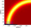Fig. 14. Straight loop simulation mapped to a semi-circular grid. Only one half of the numerical domain is shown. The emissivity, ρ2, has been passed through the SDO/AIA 171 Å temperature response function to show the intensity in that bandpass. There is no resulting intensity from the chromosphere or the transition region due to the 171 Å temperature response. Solid blue lines show LOS rays taken from the footpoint from s = 0 to 30 Mm height.

The top panel of Fig. 15 shows the intensity variations in the corona above the footpoint across the loop. As was seen in Fig. 12 of White & Verwichte (2021), an anti-symmetric oscillatory pattern with a period of 40 min can be seen between the outer and inner parts of the loop along x. The asymmetry follows from the acoustic driver being proportional to the derivative of the fast wave transverse profile. However, the pattern is further confused by the difference in distance along the loop axis covered between the outer and inner parts of the loop.

Fig. 15. Synthetic relative intensity variations in the SDO/AIA 171Å bandpass. (a) Intensity variations, averaged along a set of LOS rays as shown in Fig. 14, as a function of time, obtained numerically for an oscillation beginning at 11:19 UT. (b) Relative intensity averaged over the transverse coordinate as a function of time. The dashed line is a smooth slow trend fitted using a Savitzky-Golay filter. (c) Relative intensity as a function of time found after subtracting the slow trend. (d) Relative intensity as a function of time found after subtracting the slow trend from a time series where the relative intensity in panel (a) has been averaged only over the outer half of the loop, i.e. over the transverse interval for x between −248 and −200 Mm in the numerical domain. The dashed line is a damped sinusoidal fit.

We also observe a long-period oscillation of 81 min, which can be observed across the transverse direction and seen more clearly when averaging over the transverse direction, as shown in panel (b) of Fig. 15. This oscillation corresponds to the upflow of plasma towards the loop top due to the ponderomotive force, which has a period of P ≈ L/c_s = 82 min. By comparison, periods of 79 and 80 min were reported by White & Verwichte (2021) and Verwichte et al. (2010), respectively, which shows good agreement with predictions. The amplitude of this perturbation is 20.7%, which is larger than the amplitude of 16.2% reported by White & Verwichte (2021). This is explained by the change in the longitudinal transverse-wave mode structure in the presence of a transition region and a chromosphere.

To extract the slow mode intensity oscillations from the signal, dominated by the ponderomotive force, a smooth trend, using a Savitzky-Golay filter (Savitzky & Golay 1964), was subtracted from the overall signal. The slow mode intensity averaged across the entire loop is given in panel (c) of Fig. 15. Along with the overall 40-min period signal, there is an additional 20-min periodicity. This is a direct consequence of the anti-symmetric nature of the slow waves across the loop and the asymmetry in the LOS integration. This effect is removed by averaging and de-trending over only one half of the loop, as shown in panel (d) of Fig. 15. A damped sinusoidal curve was fitted to the data and we found an oscillation with a period of 40 min, with a negligible contribution from higher modes. We found a maximum intensity amplitude of the slow modes of 6.0%. This is similar to what was found by White & Verwichte (2021). However, this is smaller than the 15% reported by Verwichte et al. (2010). Overall, the results are similar to those already found by White & Verwichte (2021).

5.2. Simulated observation in the lower atmosphere

By omitting the SDO/AIA 171Å temperatrue response function from the calculation of intensity, that is to say, essentially calculating the emission measure ∫ρ²dz, we found that the transition region and chromosphere completely dominate the total intensity (see Fig. 16). This allows us to make a fairly crude representation of an observation made in the lower atmosphere. Figure 17 shows that there is an intensity oscillation with a period of 10 min superimposed on the 40-min oscillation. After averaging over the transverse direction, we again observed an 80-min oscillation due to the ponderomotive force. The intensity amplitude of 8.5% is smaller than the amplitude of 20.7% found in the corona.

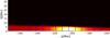Fig. 16. Straight loop simulation mapped to a semi-circular grid. Only a single footpoint is shown. The intensity is the emission measure integrated along the LOS rays. Solid blue lines show LOS rays taken from the footpoint from a height s = 0 to 8 Mm.

Again, removing the smooth trend from the fit, as shown in panel (d) of Fig. 17, we observe the typical 40-min oscillation with an additional 20-min oscillation due to the anti-symmetry, though the latter is less clear than in Fig. 15. The 10-min oscillation is completely absent. Averaging across only half the loop and again subtraction with the smooth trend, as shown in panel (e) of Fig. 17, removes the artificial 20-min oscillation and recovers the 40- and 10-min oscillations. The 10-min oscillation is likely due to the excitation of the previously mentioned hybrid slow-fast mode, which has the characteristics of a fast mode in the corona, but a slow mode in the chromosphere. These lower-period oscillations may provide an additional interesting indication of this coupling. We note that the damping within this region is likely to be significant due to a number of different processes, such as ion-neutral collisions that, along with the addition of noise in any observation due to the dynamic nature of this region, will make the detection of these waves more difficult.

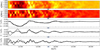Fig. 17. Synthetic relative intensity variations. (a) Intensity variations averaged along a set of LOS rays as shown in Fig. 16, as a function of time, obtained numerically for an oscillation beginning at 11:19UT. (b) Relative intensity variations from panel (a) with a smooth slow trend removed using a Savitzky-Golay filter at each transverse coordinate, x. (c) Relative intensity averaged over the transverse coordinate as a function of time, taken from the same region, as a function of time. The dashed line is a smooth, slow trend fitted using a Savitzky-Golay filter. (d) Relative intensity as a function of time found after subtracting the slow trend. The dashed line is a damped sinusoidal fit. (e) Relative intensity as a function of time found after subtracting the slow trend from a time series where the relative intensity in panel (a) has been averaged only over the outer half of the loop, i.e. over the transverse interval for x between −248 and −200 Mm in the numerical domain. The dashed line is a damped sinusoidal fit.

6. Discussion

Terradas et al. (2011) first proposed that coupling between slow magnetoacoustic and transverse (Alfvénic) waves at loop footpoints and the transition region can be used to explain intensity variations with the same periodicity as the transverse displacement. This was done using the linearised MHD equations for a uniform plasma. This model was extended to include transverse structuring in the form of a two-dimensional arcade slab in the work done by White & Verwichte (2021). We have extended this model further to include a lower atmosphere with a transition region and a chromosphere. We modelled our loop as a two-dimensional arcade slab to determine the effect of adding a transition region on the previous results obtained by White & Verwichte (2021).

We show, both numerically and analytically, that slow waves are found to be generated predominantly at the top of the transition region. They propagate at the local sound speed upwards into the corona, as well as down into the chromosphere where they ultimately reflect at the photospheric boundary. The rates of slow wave excitation are of the same order of magnitude as those found in White & Verwichte (2021) in the absence of a chromosphere. But for a transition region with a contrast ζ = 160, the rate is at least a factor of four stronger. In a realistic atmosphere with ζ of the order of 1000, we expect the excitation rate to be even larger. However, this needs to be explicitly verified. As was reported by White & Verwichte (2021), we also observe the excitation of upward propagating waves from the lower boundary, but the rate of wave excitation is lower as the excitation term is proportional to $c_{\text{Sch}}^2$, which is a factor of ζ⁻¹ smaller than at the top of the transition region and in the corona. The places of excitation correspond to regions where the coupling term has a spatial gradient, so that forward and backward excited waves do not cancel locally. We find that slow waves propagating downwards from the transition region and reflecting upwards, depending on the travel time, may destructively or constructively interfere with the upward propagating waves, which causes a decrease or increase, respectively, in the acoustic wave power in the corona. We find, as before, that the slow mode wave profile is anti-symmetric both about the loop axis and the centre of the loop. But in the presence of a transition region, additional longitudinal harmonics in the wave solution, and possibly a separate hybrid transverse mode, lead to the excited slow waves having a narrower transverse wave profile that concentrates them inside the loop.

The simulations show that a significant fraction of the total kinetic energy of the transverse oscillation may exchange between the corona and chromosphere. We believe this occurs to due to the superposition of a basic transverse mode and a hybrid mode that has characteristics of a slow wave in the chromosphere. The difference in frequency between those two types of modes is proportional to the plasma-β. A more detailed study is required, with a more realistic lower atmosphere, to confirm this. But if this superposition holds, then it has implications for the interpretation of the attenuation of transverse loop oscillations.

By forward modelling the observation of intensity at the loop footpoints made by Verwichte et al. (2010), we recovered many features previously found by White & Verwichte (2021). Variations due to the effect of the ponderomotive force dominate the signal, as predicted, for an initial perturbation of the order of tenths of the Alfvén speed. The intensity oscillations of the excited slow waves is recovered once the ponderomotive effect on the time series is subtracted. However, due to the transverse anti-symmetry of the slow waves, integration of the signal across the whole loop cross-section leads to a reduction in the wave mode amplitude and the appearance of spurious double harmonics. Therefore, observations have to have sufficient spatial resolution to resolve the loop width, and they have to be carefully analysed to reveal the slow waves. The synthetic observation also shows that in the lower atmosphere, besides the typical intensity variations with a periodicity equal to the transverse oscillation, there is an additional short-period oscillation. This may provide another potential signature of slow mode coupling. This is believed to be due to the presence of the additional hybrid mode.

In our loop model, we assumed no variation in plasma-β along the loop so that the density increases as the temperature decreases, while the magnetic field along the loop remains constant. To obtain a more realistic transition region, we would require a larger density contrast between the corona and the chromosphere. Given the temperature profile, this would require an increasingly concentrated magnetic field to allow for total pressure balance. Furthermore, simulations of a realistic transition region would require a larger number of grid points, limiting any analysis by runtime, although methods have been implemented by others to reduce this (Johnston et al. 2020). In this work and in previous works, the temperature is constant across the loop, while for a real loop, we would expect some variation. This would lead to a varying sound speed across the loop, which in turn would lead to a phase difference between those slow magnetoacoustic waves inside and outside the loop. As was discussed by White & Verwichte (2021), any complete study of this coupling would be done in three dimensions in cylindrical geometry, allowing for the inclusion of resonant absorption.

Acknowledgments

S.J.W. acknowledges the support of the UK STFC Ph.D. studentship.

References

All Figures

Fig. 1. Transverse wave mode solutions for χ = 0.1. Top: dispersion plot, showing the solutions of Eq. (14) for χ = 0.1 as the normalised phase speed vph/vAi versus the normalised wave number ka, for the first eleven transverse harmonics. Solid (dashed) curves indicate trapped (leaky) modes. The normalised internal and external Alfvén speeds are indicated by dashed black lines. Bottom: normalised transverse displacement profile Pn(tanh(x/a)) sechα(x/a) as a function of x/a for three modes whose phase speed and wave number are indicated as coloured circles above. The solid (dashed) curves are the real (imaginary) part.

In the text

Fig. 2. Structure of a given mode solution for the lowest frequency mode. Top left: relative Alfvén speed as a function of transverse and longitudinal coordinates, x and y, respectively, for the parameters values of χ = 0.1, ζ = 160, L = 252 Mm, a = 5 Mm, y0 = 6 Mm, and Δy = 1 Mm. The horizontal dashed lines indicate x = ±a. Top right: real part of the fundamental transverse eigenmode, ${\widehat{\xi }}_{\perp }$. The subsequent panels show some of the individual basic modes ${\widehat{\xi }}_{\perp ,m,n}$ that contribute to the full eigenmode. The relative amplitudes of those basic modes relative to ${\widehat{\xi }}_{\perp ,1,0}$ are given.

In the text

Fig. 3. Transverse structuring of the fundamental transverse eigenmode. Top: real part of the fundamental transverse eigenmode as a function of transverse and longitudinal coordinates, x and y, respectively, from which the basic mode with longitudinal wave number m = 1 and transverse wave number n = 0 is subtracted, ${\widehat{\xi }}_{\perp }-{\widehat{\xi }}_{\perp ,1,0}$. The physical parameters are the same as for Fig. 2. Bottom: normalised transverse wave profile of the derivative of the fundamental transverse eigenmode, df/dx, as a function of x for three positions in y along the loop: 0 (red), y0 + Δy (blue), and L/2 (black).

In the text

Fig. 4. Spatial profiles across the transition region of the equilibrium mass density, ρ0(y)/ρ0c, Alfvén speed, vA(y), transverse displacement, ξ⊥/ξ0, derivative of the transverse displacement, ∂/∂y(ξ⊥/ξ0), the acoustic coupling term, $c_{\text{S}}{}^2(y)k_{\perp }\partial /\partial y\left({\xi }_{\perp }/{\xi }_0\right)$, and the longitudinal displacement, ξ∥/ξ0. The vertical dashed and dotted lines indicate the positions y0 and y0 ± Δy, respectively. The blue and red curves are the wave solutions for a density contrast ζ = 10 and 1000, respectively.

In the text

References

- Abramowitz, M., & Stegun, I. A. 1965, Handbook of Mathematical Functions with Formulas, Graphs, and Mathematical Tables (National Bureau of Standards) [Google Scholar]
- Andries, J., Arregui, I., & Goossens, M. 2005, ApJ, 624, L57 [NASA ADS] [CrossRef] [Google Scholar]
- Andries, J., Arregui, I., & Goossens, M. 2009, A&A, 497, 265 [NASA ADS] [CrossRef] [EDP Sciences] [Google Scholar]
- Arber, T. D., Longbottom, A. W., Gerrard, C. L., & Milne, A. M. 2001, J. Comput. Phys., 171, 151 [NASA ADS] [CrossRef] [Google Scholar]
- Arregui, I., Terradas, J., Oliver, R., & Ballester, J. L. 2008, ApJ, 674, 1179 [NASA ADS] [CrossRef] [Google Scholar]
- Aschwanden, M. J., & Schrijver, C. J. 2011, ApJ, 736, 102 [NASA ADS] [CrossRef] [Google Scholar]
- Aschwanden, M. J., Fletcher, L., Schrijver, C. J., & Alexander, D. 1999, ApJ, 520, 880 [Google Scholar]
- Berghmans, D., Clette, F., Robbrecht, E., & McKenzie, D. 1999, ESA Spec. Publ., 9, 575 [Google Scholar]
- Bourdin, P. A., Bingert, S., & Peter, H. 2013, A&A, 555, A123 [NASA ADS] [CrossRef] [EDP Sciences] [Google Scholar]
- Cooper, F. C., Nakariakov, V. M., & Tsiklauri, D. 2003, A&A, 397, 765 [CrossRef] [EDP Sciences] [Google Scholar]
- Davila, J. M. 1991, in Mechanisms of Chromospheric and Coronal Heating, eds. P. Ulmschneider, E. R. Priest, & R. Rosner (New York: Springer), 464 [CrossRef] [Google Scholar]
- De Moortel, I. 2006, Philos. Trans. R Soc. London Ser. A, 364, 461 [Google Scholar]
- De Moortel, I., Ireland, J., & Walsh, R. W. 2000, A&A, 355, L23 [NASA ADS] [Google Scholar]
- De Pontieu, B., Martens, P. C. H., & Hudson, H. S. 2001, ApJ, 558, 859 [Google Scholar]
- Díaz, A. J. 2006, A&A, 456, 737 [NASA ADS] [CrossRef] [EDP Sciences] [Google Scholar]
- Dymova, M. V., & Ruderman, M. S. 2006, A&A, 457, 1059 [NASA ADS] [CrossRef] [EDP Sciences] [Google Scholar]
- Edwin, P. M., & Roberts, B. 1983, Sol. Phys., 88, 179 [Google Scholar]
- Epstein, P. S. 1930, PNAS, 16, 627 [NASA ADS] [CrossRef] [Google Scholar]
- Fletcher, L., & Hudson, H. S. 2008, ApJ, 675, 1645 [Google Scholar]
- Gary, G. A. 2001, Sol. Phys., 203, 71 [Google Scholar]
- Goddard, C. R., & Nakariakov, V. M. 2016, A&A, 590, L5 [NASA ADS] [CrossRef] [EDP Sciences] [Google Scholar]
- Goedbloed, J. P., & Halberstadt, G. 1994, A&A, 286, 275 [NASA ADS] [Google Scholar]
- Goossens, M., Andries, J., & Aschwanden, M. J. 2002, A&A, 394, L39 [NASA ADS] [CrossRef] [EDP Sciences] [Google Scholar]
- Goossens, M., Erdélyi, R., & Ruderman, M. S. 2011, Space Sci. Rev., 158, 289 [Google Scholar]
- Haerendel, G. 2009, ApJ, 707, 903 [NASA ADS] [CrossRef] [Google Scholar]
- Heyvaerts, J., & Priest, E. R. 1983, A&A, 117, 220 [NASA ADS] [Google Scholar]
- Hollweg, J. V. 1984, ApJ, 277, 392 [Google Scholar]
- Ionson, J. A. 1978, ApJ, 226, 650 [NASA ADS] [CrossRef] [Google Scholar]
- Jess, D. B., Reznikova, V. E., Ryans, R. S. I., et al. 2016, Nat. Phys., 12, 179 [NASA ADS] [CrossRef] [Google Scholar]
- Johnston, C. D., Cargill, P. J., Hood, A. W., et al. 2020, A&A, 635, A168 [NASA ADS] [CrossRef] [EDP Sciences] [Google Scholar]
- Kumar, P., Innes, D. E., & Inhester, B. 2013, ApJ, 779, L7 [Google Scholar]
- Kumar, P., Nakariakov, V. M., & Cho, K.-S. 2015, ApJ, 804, 4 [NASA ADS] [CrossRef] [Google Scholar]
- Lemen, J. R., Title, A. M., Akin, D. J., et al. 2012, Sol. Phys., 275, 17 [Google Scholar]
- Li, D., Ning, Z. J., Huang, Y., et al. 2017, ApJ, 849, 113 [NASA ADS] [CrossRef] [Google Scholar]
- Nakariakov, V. M., & Ofman, L. 2001, A&A, 372, L53 [NASA ADS] [CrossRef] [EDP Sciences] [Google Scholar]
- Nakariakov, V. M., & Roberts, B. 1995, Sol. Phys., 159, 399 [NASA ADS] [CrossRef] [Google Scholar]
- Nakariakov, V. M., & Verwichte, E. 2005, Liv. Rev. Sol. Phys., 2, 3 [Google Scholar]
- Nakariakov, V. M., Ofman, L., Deluca, E. E., Roberts, B., & Davila, J. M. 1999, Science, 285, 862 [Google Scholar]
- Nisticò, G., Polito, V., Nakariakov, V. M., & Del Zanna, G. 2017, A&A, 600, A37 [NASA ADS] [CrossRef] [EDP Sciences] [Google Scholar]
- Reep, J. W., Russell, A. J. B., Tarr, L. A., & Leake, J. E. 2018, ApJ, 853, 101 [NASA ADS] [CrossRef] [Google Scholar]
- Robbrecht, E., Verwichte, E., Berghmans, D., et al. 2001, A&A, 370, 591 [NASA ADS] [CrossRef] [EDP Sciences] [Google Scholar]
- Roberts, B. 2019, MHD Waves in the Solar Atmosphere (Cambridge University Press) [Google Scholar]
- Ruderman, M. S., & Roberts, B. 2002, ApJ, 577, 475 [Google Scholar]
- Russell, A. J. B., & Stackhouse, D. J. 2013, A&A, 558, A76 [NASA ADS] [CrossRef] [EDP Sciences] [Google Scholar]
- Savitzky, A., & Golay, M. J. E. 1964, Anal. Chem., 36, 1627 [Google Scholar]
- Terradas, J., Andries, J., & Verwichte, E. 2011, A&A, 527, A132 [NASA ADS] [CrossRef] [EDP Sciences] [Google Scholar]
- Van Doorsselaere, T., Srivastava, A. K., Antolin, P., et al. 2020, Space Sci. Rev., 216, 140 [Google Scholar]
- Verth, G., Van Doorsselaere, T., Erdélyi, R., & Goossens, M. 2007, A&A, 475, 341 [NASA ADS] [CrossRef] [EDP Sciences] [Google Scholar]
- Verwichte, E., & Kohutova, P. 2017, A&A, 601, L2 [NASA ADS] [CrossRef] [EDP Sciences] [Google Scholar]
- Verwichte, E., Foullon, C., & Nakariakov, V. M. 2006, A&A, 446, 1139 [NASA ADS] [CrossRef] [EDP Sciences] [Google Scholar]
- Verwichte, E., Aschwanden, M. J., Van Doorsselaere, T., Foullon, C., & Nakariakov, V. M. 2009, ApJ, 698, 397 [NASA ADS] [CrossRef] [Google Scholar]
- Verwichte, E., Foullon, C., & Van Doorsselaere, T. 2010, ApJ, 717, 458 [NASA ADS] [CrossRef] [Google Scholar]
- Verwichte, E., Van Doorsselaere, T., Foullon, C., & White, R. S. 2013, ApJ, 767, 16 [Google Scholar]
- Voitenko, Y., Andries, J., Copil, P. D., & Goossens, M. 2005, A&A, 437, L47 [NASA ADS] [CrossRef] [EDP Sciences] [Google Scholar]
- Wang, T. J., & Solanki, S. K. 2004, A&A, 421, L33 [NASA ADS] [CrossRef] [EDP Sciences] [Google Scholar]
- Wang, T. J., Solanki, S. K., Curdt, W., et al. 2003a, A&A, 406, 1105 [NASA ADS] [CrossRef] [EDP Sciences] [Google Scholar]
- Wang, T. J., Solanki, S. K., Innes, D. E., Curdt, W., & Marsch, E. 2003b, A&A, 402, L17 [NASA ADS] [CrossRef] [EDP Sciences] [Google Scholar]
- White, R. S., & Verwichte, E. 2012, A&A, 537, A49 [NASA ADS] [CrossRef] [EDP Sciences] [Google Scholar]
- White, R. S., Verwichte, E., & Foullon, C. 2012, A&A, 545, A129 [NASA ADS] [CrossRef] [EDP Sciences] [Google Scholar]
- White, S. J., & Verwichte, E. 2021, A&A, 654, A33 [NASA ADS] [CrossRef] [EDP Sciences] [Google Scholar]
- Yuan, D., & Van Doorsselaere, T. 2016, ApJS, 223, 24 [NASA ADS] [CrossRef] [Google Scholar]