| Issue |
A&A
Volume 667, November 2022
|
|
|---|---|---|
| Article Number | A42 | |
| Number of page(s) | 20 | |
| Section | Extragalactic astronomy | |
| DOI | https://doi.org/10.1051/0004-6361/202243194 | |
| Published online | 03 November 2022 | |
Wavelength-resolved reverberation mapping of quasar CTS C30.10: Dissecting Mg II and Fe II emission regions
1
Center for Theoretical Physics, Polish Academy of Sciences, Al. Lotników 32/46, 02-668 Warsaw, Poland
e-mail: This email address is being protected from spambots. You need JavaScript enabled to view it.
2
Department of Theoretical Physics and Astrophysics, Faculty of Science, Masaryk University, Kotlářská 2, 61137 Brno, Czech Republic
3
Centre for Astrophysics and Cosmology, University of Nova Gorica, Vipavska 11c, 5270 Ajdovščina, Slovenia
4
Astronomisches Institut Ruhr-Universitat Bochum, Universitatsstrae 150, 44801 Bochum, Germany
5
Nicolaus Copernicus Astronomical Center, Polish Academy of Sciences, ul. Bartycka 18, 00-716 Warsaw, Poland
6
Laboratório Nacional de Astrofísica, R. dos Estados Unidos, 154 - Nacões, Itajubá, MG 37504-364, Brazil
7
Departamento de Astronomia, Universidad de Chile, Camino del Observatorio 1515, Santiago, Chile
8
National Centre for Nuclear Research, ul. Pasteura 7, 02-093 Warsaw, Poland
9
Astronomical Institute, Academy of Sciences, Boční II 1401, 14131 Prague, Czech Republic
10
Space Research Center, Polish Academy of Sciences, Bartycka 18A 00-716, Warszawa, Poland
11
Astronomical Observatory of the Jagiellonian University, Orla 171, 30-244 Krakow, Poland
12
Warsaw University Observatory, Al. Ujazdowskie 4, 88-478 Warsaw, Poland
13
outh African Astronomical Observatory, PO Box 9 Observatory, 7935 Cape Town, South Africa
14
University of Cape Town, Rondebosch, 7700 Cape Town, South Africa
Received:
25
January
2022
Accepted:
9
June
2022
Abstract
Context. We present the results of the reverberation monitoring of the Mg II broad line and Fe II pseudocontinuum for the luminous quasar CTS C30.10 (z = 0.90052) with the Southern African Large Telescope in 2012–2021.
Aims. We aimed at disentangling the Mg II and UV Fe II variability and the first measurement of UV Fe II time delay for a distant quasar.
Methods. We used several methods for the time-delay measurements and determined the Fe II and Mg II time delays. We also performed a wavelength-resolved time delay study for a combination of Mg II and Fe II in the 2700–2900 Å rest-frame wavelength range.
Results. We obtain a time delay for Mg II of 275.5−19.5+12.4 days in the rest frame, and we have two possible solutions of 270.0−25.3+13.8 days and 180.3−30.0+26.6 in the rest frame for Fe II. Combining this result with the old measurement of Fe II UV time delay for NGC 5548, we discuss for first time the radius-luminosity relation for UV Fe II with the slope consistent with 0.5 within the uncertainties.
Conclusions. Because the Fe II time delay has a shorter time-delay component but the lines are narrower than Mg II, we propose that the line-delay measurement is biased toward the part of the broad line region (BLR) facing the observer. The bulk of the Fe II emission may arise from the more distant BLR region, however, the region that is shielded from the observer.
Key words: accretion, accretion disks / quasars: emission lines / quasars: individual: CTS C30.10 / techniques: spectroscopic / techniques: photometric
© R. Prince et al. 2022
 Open Access article, published by EDP Sciences, under the terms of the Creative Commons Attribution License (https://creativecommons.org/licenses/by/4.0), which permits unrestricted use, distribution, and reproduction in any medium, provided the original work is properly cited.
This article is published in open access under the Subscribe-to-Open model. This email address is being protected from spambots. You need JavaScript enabled to view it. to support open access publication.
1. Introduction
It is now widely accepted that the central engine of an active galactic nucleus (AGN) consists of the central supermassive black hole (SMBH) and the accretion disk around it (see Krolik 1999; D’Onofrio et al. 2012; Karas et al. 2021, 2022, for reviews). Recent observations by the Event Horizon Telescope (EHT) collaboration of the nearest jetted AGN, M87 provided elegant proof that the AGN carries a Kerr SMBH of (6.5 ± 0.7) ×109 M⊙ (EHT Collaboration 2019a,b). This is also the case of extremely low-luminous systems, such as Sgr A*, the closest galactic nucleus to Earth, where the bound orbits of S stars and dusty objects provide evidence of a compact mass of ∼4 × 10⁶ M⊙ (Boehle et al. 2016; Gillessen et al. 2017; Parsa et al. 2017; Eckart et al. 2017; GRAVITY Collaboration 2018a, 2020a; Peißker et al. 2020a,b).
However, despite our increasing knowledge, we have a much less detailed understanding of the properties of the plasma or gas and dust located farther away from the SMBH, at a fraction of a parsec and more. This material causes the characteristic broad emission lines coming from the broad line region (BLR) and also the infrared emission originating in the dusty or molecular torus (see Netzer 2015, for a review). Broad emission lines from the BLR are the most characteristic features in the optical and UV spectra of bright type I AGN (Seyfert 1943; Woltjer 1959; Schmidt 1963) that are viewed close to the symmetry axis of the system, including quasars. For type II AGN, no broad lines are not visible in direct unpolarized light due to the obscuration by the thick dusty molecular torus. However, they can be revealed in polarized emission through scattering (the type II AGN NGC1068 was the first such a case that revealed broad Balmer lines, see Antonucci & Miller 1985), which led to the unification scheme of AGN in which different viewing angles reveal different structures of the nuclear engine (Antonucci 1993; Urry & Padovani 1995).
Generally, the velocity width of the broad emission lines varies from source to source, and previous studies suggested that it might be between ∼103 km s−1 to ∼104 km s−1 (Schmidt 1963; Osterbrock & Mathews 1986; Boroson & Green 1992; Sulentic et al. 2000; Shen et al. 2011). The large emission-line widths in the BLR are caused by the cloud motion, specifically, the Doppler broadening, while the radiative process that causes the broad-line emission apparently arises from the photoionization by the X-ray/UV radiation of the inner accretion disk, as implied by the significant correlation and the associated time delay of the emission-line light curve with respect to the changes in the irradiating continuum. So-called reverberation mapping (RM) studies have successfully been performed by now for more than one hundred objects (e.g. Liutyi & Pronik 1975; Kaspi et al. 2000; Peterson et al. 2004; Bentz et al. 2013; Mejía-Restrepo et al. 2018; Grier et al. 2017; Du et al. 2018a; Yu et al. 2021).
The BLR is basically unresolved, except for the most recent measurements in the near-infrared domain (K band, 2.2 μm) that were performed for three AGN (3C273, IRAS 09149-6206, and NGC 3783) with the infrared instrument GRAVITY at the Very Large Telescope Interferometer (GRAVITY Collaboration 2018b, 2019, 2020b, 2021), which spatially resolved near-infrared broad hydrogen lines. These spatially resolved BLR detections confirmed that the BLR is best represented by a thick-disk system that rotates around the central source under the influence of the central SMBH. Hence, the GRAVITY observations have justified the RM method for studying the dynamics of BLR and the SMBH. This technique has been extensively employed in AGN to measure the time lags between two causally connected light curves. The measured time lags can be directly linked to the physical size of the system via the speed of light. There are three types of RM: BLR-RM, X-ray-RM, and the continuum RM that is mainly seen in AGN (Cackett et al. 2021). It was first proposed by Blandford & McKee (1982) and Peterson (1993), and later it was widely used to estimate the size of the BLR, the accretion-disk size, and the structure as well as the SMBH mass in AGN and quasars (Kaspi et al. 2000, Peterson et al. 2004, Mejía-Restrepo et al. 2018). Recently, it has been discovered that the time delay estimated from the RM can also be used to estimate the luminosity distance of the AGN, which can eventually be used to constrain the cosmological parameters (Watson et al. 2011; Haas et al. 2011; Czerny et al. 2013, 2021; Martínez-Aldama et al. 2019, 2020a; Panda et al. 2019; Zajaček et al. 2021; Khadka et al. 2021, 2022). In addition to the UV, optical, and infrared broad lines, the BLR is a prospective source of the nonthermal emission because the clouds that have been lifted off the accretion disk later fall back and collide with the disk with impact velocities from a few km s−1 up to ∼1000 km s−1. These collisions induce strong shocks that accelerate particles to relativistic energies and eventually produce steady X-ray and γ-ray emission (Müller et al. 2022).
Studies of the BLR line widths combined with the RM have clearly shown several important properties of the BLR (see, e.g., Wandel et al. 1999; Gaskell 2009; Li et al. 2013; Pancoast et al. 2014; Grier et al. 2017): (i) a considerable stratification of the line-emitting material and (ii) a prevailing Keplerian motion, confined to the accretion-disc plane, but with an additional inflow/outflow or turbulent component. GRAVITY/VLT observations nicely confirmed the conclusion about the overall flatness of the BLR configuration deduced previously from spectral and variability studies.
Simple time-delay measurements of a single emission line do not give much information about the BLR structure, except for the mean (effective) radius of the emission. More information comes from studies of many emission lines in a given source and/or from velocity-resolved measurements (Done & Krolik 1996; Wandel et al. 1999; Bentz et al. 2010; Denney et al. 2010; Grier et al. 2012; De Rosa et al. 2015, 2018; Lu et al. 2016; Pei et al. 2017; Du et al. 2018a; Xiao et al. 2018; Zhang et al. 2019; Hu et al. 2020; Horne et al. 2021; Vivian et al. 2022). These studies have been conducted for relatively nearby sources so far, for selected objects, including the extensively monitored source NGC 5548. This method can reveal the velocity structure of the medium, and therefore it is most suitable not only to obtain most reliable measurement of the time delays of specific lines and establish the inflow or outflow pattern that is superimposed on the circular motion, but also to determine time delays of broader pseudo-continua, such as the optical Fe II and particularly for UV Fe II pseudo-continuum, which strongly overlaps with the Mg II line. The optical Fe II time delay has indeed been measured in a few lower-redshift sources (Bian et al. 2010; Barth et al. 2013; Hu et al. 2015, 2020; Zhang et al. 2019).
Monitoring of more distant objects is in general less frequent, but basic time-delay measurements in distant quasars were performed on the Mg II line (Metzroth et al. 2006; Shen et al. 2016; Czerny et al. 2019; Zajaček et al. 2020, 2021; Lira et al. 2018; Homayouni et al. 2020; Yu et al. 2021) and CIV line (Peterson et al. 2005, 2006; Metzroth et al. 2006; De Rosa et al. 2015; Lira et al. 2018; Hoormann et al. 2019; Grier et al. 2019; Shen et al. 2019; Kaspi et al. 2021; Penton et al. 2022). In our previous paper about the luminous quasar CTS C30.10, we reported the long-term measurement of Mg II emission (Czerny et al. 2019). The reverberation mapping result using various methods revealed a time delay of 562 days (rest frame) between the 3000 Å continuum and the Mg II line variations in this source. This result suggests that the radius-luminosity relation derived from the Mg II matches previous results from the Hβ line. In addition, using the sample of 68 Mg II quasars, we demonstrated that the scatter along the radius-luminosity relation is mostly driven by the accretion rate intensity (Martínez-Aldama et al. 2020b).
The aim of the current paper is the first determination of the time delay of UV Fe II with respect to the continuum. Our study is based on eight years of spectroscopic data for quasar CTS C30.10 with the dedicated monitoring with the Southern African Large Telescope (SALT). We have determined the Mg II time delay in this source earlier, on the basis of shorter data (∼6 yr) (Czerny et al. 2019). Because the UV Fe II and Mg II decomposition may be biased by the choice of template, we performed a wavelength-resolved analysis for this source.
Velocity-resolved spectroscopy is an important tool and can be used to explore the relation between the emission line variations and their velocity information. It can also be used to estimate the mass of the central SMBH. In the past, this method has been applied to more than 35 AGNs by various authors (Bentz et al. 2010; Denney et al. 2010; Grier et al. 2012; Du et al. 2018a; De Rosa et al. 2018; Xiao et al. 2018; Zhang et al. 2019; Hu et al. 2020; Vivian et al. 2022).
The paper is structured as follows. In Sect. 2 we describe spectroscopic and photometric data and their reduction. We determine the mean and the RMS spectra, and construct Mg II, Fe II, and wavelength-resolved light curves in Sect. 3. Subsequently, in Sect. 4, we analyze the continuum and the emission-line variability, and we present the Mg II and the Fe II time delays as well as the wavelength-resolved reverberation mapping of the Mg II+Fe II complex. In Sect. 5 we discuss the implications for the BLR kinematics and we show the updated Mg II radius-luminosity relation as well as the first construction of the UV Fe II radius-luminosity relation. Finally, we summarize the main conclusions in Sect. 6.
2. Observations and data reduction
The source CTS C30.10 is a bright (V = 17.2 mag, NED) quasar in the southern part of the sky identified in the Calan–Tololo Survey (Maza et al. 1988, 1993). It is located at a redshift of z = 0.90052 (Modzelewska et al. 2014) with RA = 04h47m19.9s, Dec = −45d37m38.0s (J2000.0). We have monitored this quasar since December 2012, and the last observation was made on 2021 March 25. Long-term photometric and spectroscopic data are used in this study. In almost nine years of observations, the source has been visited 36 times by the SALT telescope, and therefore we have 36 observations. Observation number 6 was obtained on 2014 August 17 and was identified as an outlier. It was eventually dropped from the further study. Therefore, the study presented here is based on 35 SALT visits.
2.1. Spectroscopy
The spectroscopic observational setup is similar to what is described in Czerny et al. (2019). Here, we have 36 observations, each observation consisting of two observing blocks with an exposure of almost 800 s. The details of the first 26 observations are provided in Czerny et al. (2019) (Table-1)1. We here present only the later observations in Table 1. Observation 18 in Czerny et al. (2019) was removed because it is a strong outlier. We here properly calibrated observation 18 and found that it contains reliable data. We therefore use this observation here. However, observation 6 is still an outlier (due to very poor weather conditions) and was not considered in the present work. The reduction of raw SALT data was made by SALT telescope staff using the standard pipeline (Crawford et al. 2010), and the further procedure of the data reduction is described in Czerny et al. (2019) in detail. To correct for the vignetting effects in the SALT spectra, a proper calibration with the use of a standard star was made. A detailed description of the procedure is given in the Sect. 2.1 of Modzelewska et al. (2014).
Results of the data fitting to SALT spectroscopy, starting from observation 27.
2.2. Mg II line fitting
The reduced and calibrated spectra were model with all possible components, including the continuum power law (disk emission), the Fe II pseudo-continuum, and two components of the Mg II emission line. The Fe II and Mg II emission lines are expected to be produced in the BLR. The spectra cover a wide range of wavelengths from 2700–2900 Å in the rest frame of the source. As suggested by Modzelewska et al. (2014), the Fe II pseudo-continuum was modeled by the empirical template d12-m20-20-5 provided by Bruhweiler & Verner (2008) with a cloud number density of 1012 cm−3, and a microturbulence velocity of 20 km s−1, and the flux of hydrogen-ionizing photons above 13.6 eV is assumed to be 10+20.5 cm−2 s−1. The Fe II template was further convolved with a Gaussian profile with a width of 900 km s−1 considering the broadening in the Fe II lines.
Detailed modeling of Mg II components is discussed in Modzelewska et al. (2014). These authors tried various ways to fit the Mg II emission lines, including one single component, two separate emission components, and a single component with the absorption. Here, we fit the Mg II emission lines with two different components assuming that both components are described by a Lorentzian shape profile. We also tried the Gaussian profile, but the χ2 values were high compared to a Lorentzian profile. An exemplary spectrum fit with power law, Fe II, and Mg II components is shown in Fig. 1.
 |
Fig. 1. Observation 36 from the SALT telescope (red) and the model (black). The dashed green line shows the underlying continuum from the accretion disk, the dotted blue line is the Fe II pseudo-continuum, and the dotted magenta lines represent the two kinematic components of the Mg II line. |
The total equivalent width (EW) of the lines and their error bars for the first 26 observations are presented in Czerny et al. (2019), and the rest of the observations are shown in the Table 1 of this work. Detailed descriptions of the parameters can be found in Czerny et al. (2019). In Table 2 we present all the observations and inferred Mg II and Fe II flux densities after fitting the corresponding emission lines as well as the continuum power-law emission component.
Estimated fluxes in Mg II and Fe II along with their errors.
2.3. Photometry
The photometric observations of the source have been obtained with various telescopes throughout the globe. Our aim was to have the photometric observations close in time to spectroscopy by SALT, and hence in this regard we alerted many telescopes. The early part of the photometry has been described in Czerny et al. (2019), who used photometric points from four telescopes (the CATALINA survey for the very early observations prior to our monitoring, and later OGLE, SALTICAM SALT, and BMT of the Observatorio Cerro Armazones, OCA). Here we include new data from SALTICAM SALT and BMT, as well as the data from four additional telescopes: Las Cumbres at the Siding Spring Observatory (SSO) in Australia, SAAO (Lesedi Telescope), Las Cumbres at the Cerro Tololo Inter-American Observatory (CTIO), and Las Cumbres SAAO. There were small systematic shifts between the data from different telescopes, therefore we corrected gray shift. Because some of the newly included photometry partially covers the time span covered by photometry given in Czerny et al. (2019), we include the full photometry (except for the CATALINA data) in Table B.2. The resulting photometric curve is relatively smooth, but has a clear variability pattern (see Fig. 2). We have included more recent photometric data than Czerny et al. (2019) and calibrated all photometric data together, which slightly changes the photometric flux compared to the previous photometric fluxes reported in Czerny et al. (2019).
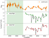 |
Fig. 2. Long-term photometric light curve (upper panel), including CATALINA measurements (light green shaded region) from Czerny et al. (2019), and total Mg II (middle panel) and Fe II (lower panel) light curves. Photometric observations are in magnitudes (panel 1), but Mg II and Fe II fluxes are in units of 10−16 and 10−17 erg s−1 cm−2. We used only the non-shaded region. |
3. Measurements
3.1. Mean and RMS spectra
To characterize the spectral behavior and the amplitude variation at different wavelengths, we also plot the mean and the root mean square (rms) spectra of the source. The mean and rms spectra are defined as
 (1)
(1)
and
![Mathematical equation: $$ \begin{aligned} S_{\lambda } = \left[ \sum _{i = 1}^{N} \left({F}_{\lambda }^{i} - \bar{F}_{\lambda }\right)^2 \right]^{1/2}, \end{aligned} $$](/articles/aa/full_html/2022/11/aa43194-22/aa43194-22-eq6.gif) (2)
(2)
where  is the ith spectrum and N is the number of spectra.
3.2. MgII and FeII light curves
The light curves for the Mg II and Fe II were created as in our previous papers (Czerny et al. 2019; Zajaček et al. 2020, 2021). Each spectrum was decomposed as described in Sect. 2.2. Each spectrum was then normalized using the photometric data because SALT spectroscopy does not allow for reliable spectrophotometric measurements directly. The final Mg II and Fe II flux was computed by subtracting the power-law component and the Fe II or Mg II component, correspondingly. The resulting light curves are shown in the middle and bottom panel of Fig. 2. Observations 9, 17, 18, and 26 appear to be outliers. However, we cross-checked the procedure and their spectrum, and they appear to be correct. To assess to which extent these observations affect the Mg II and Fe II time-delay measurements, we removed these points and checked the time-delay determinations. The time delay does not change significantly after the removal, although the correlation between the continuum and Mg II light curves increases. We discuss the implications of this analysis in Sect. 4.2 and in Appendix B.
3.3. Wavelength-resolved light curves
We followed the Hu et al. (2020) method to divide the light curves according to the flux distribution in the flux rms spectrum. However, the Hu et al. (2020) method was performed for Hβ, and in this paper we present it for the Mg II and Fe II emission. After fitting the spectroscopic data with the full model, consisting of the power-law continuum, Fe II and Mg II, we subtracted the power-law component from the data in each data set. We then constructed the rms spectrum, and we divided the spectrum into seven bins of equal fluxes. We used fewer bins than in Hu et al. (2020) because our data are of lower quality. We used the wavelength instead of the velocity because we kept a combined contribution of Mg II and Fe II in the remaining spectrum because the two components overlap significantly. The separation of Mg II and Fe II is not unique, as we discussed in Zajaček et al. (2020) because it depends on the adopted template, and we hope to gain additional insight into their separation directly from variability. These wavelength bins were later used to create seven light curves from each original spectrum, again after subtracting the best-fit power-law and integrating each spectrum within the appropriate limits.
4. Results
Our light curve of CTS C30.10 is relatively long (over eight years in the observed frame) in comparison with the time delay of three years in the observed frame that was claimed in the previous paper (Czerny et al. 2019), which allows for much better analysis. However, the overall source variability is still not much higher than before, which supports the view that the frequency break in the power spectra of quasars is typically one to two years (e.g. Kozłowski 2016; Stone et al. 2022), and the variability amplitude rises much more slowly with a longer observing time. This saturation of the amplitude was already well seen in CTS C30.10 in the previous data (see Fig. 15 of Czerny et al. 2019).
4.1. Variability
The strength of the variability can be quantified by the excess variance (σXS) and the fractional rms variability amplitude, Fvar (Edelson et al. 2002). The σXS is the measurement of the intrinsic variability in the quasar, and it is estimated by correcting the total observed light curve with measurement errors. Fvar is the square root of the σXS normalized by the mean flux value.
The fractional variability is used to characterize the long-term variability in various bands. Its functional form and error on Fvar are taken from Vaughan et al. (2003),
 (3)
(3)
where F denotes the mean flux value, fi is the individual measurement, and err is the error in the observed flux. The expression for the error on Fvar is provided in Prince (2019). We also estimated the point-to-point variability, which indicates the variability at the shortest timescales. Considering the light curve is denoted by the fi, where i = 1, 2, 3, …, N, the point-to-point variability is defined as
 (4)
(4)
The results are given in Table 3. As expected, the continuum shows less variability than the individual curves. Curves 1, 2, 3, and 7 have a variability of more than 10% in linear scale, and curves 4, 5, and 6, which are dominated by the Mg II and Fe II contribution, show a variability below 10%. The lower fractional variability is also visible in the total Mg II and Fe II emission consistence with the curves 4, 5, and 6. Furthermore, to determine the short-scale variability, we estimated Fpp for all the curves. For individual curves with a high signal-to-noise ratio, Fpp is about the same as Fvar. This confirms that the measurements are not dominated by the measurement errors because for the white noise Fpp = 1.4 Fvar, but variations are quite strong on the shortest timescales. This fast variability is not seen in the continuum, because for the continuum, Fpp is equal zero. Therefore, these fast variations are not a response to the continuum. Either the emission lines show short-timescale intrinsic variations, or we underestimate the measurement errors. Both these effects are the potential sources of the problem, and lead to a scatter in the line-continuum relation. The poor correlation between the illuminating hard-energy photons and the response of the line is frequently seen in many sources (e.g. Gaskell et al. 2021), although it is best documented in the monitoring of NGC 5548 (Goad et al. 2016; Gaskell et al. 2021).
Variability amplitude for all the curves and the continuum.
4.2. Time delay measurement in total Mg II and Fe II
We applied several standard methods that are described in more detail in Appendix A.1. The time-delay evaluation using the standard interpolated cross-correlation function (ICCF) indicates a moderately longer peak time delay for the Mg II broad line,  days in the observer’s frame, in comparison with the Fe II pseudo-continuum,
  days (see Table 4). Interestingly, the correlation coefficient at the peak is higher for the Fe II pseudo-continuum, r = 0.65 versus r = 0.55 for the Mg II line, which is also visible in Fig. 3, where we plot the ICCF as a function of the time delay for both lines. We stress that due to the large data set (continuum points and line-emission measurements), the overall time-delay peak became smaller. Previously, Czerny et al. (2019) reported a Mg II time delay of ∼1050 days in the observer’s frame. We compare the previous and current ICCF in Fig. 3. The shift of the best-fit time delay is due to the change in the relative importance of the peaks in the multipeak solution. We still see a trace of the 1050 days delay, but the shorter time delay now has a higher significance.
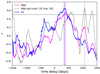 |
Fig. 3. Interpolated cross-correlation function as a function of the time delay in the observer’s frame for the total Mg II (magenta line) and the total Fe II emission (blue line). The dashed vertical lines mark the corresponding time-delay peak values. The correlation coefficient at the peak value for the Fe II pseudo-continuum is larger than the correlation coefficient at the time-delay peak of the Mg II line. The dotted horizontal line marks r = 0.5. We also show the previous ICCF (Czerny et al. 2019) when the peak time delay was at ∼1064 days; see the solid gray line. Cont:79 and line:26 represents the number of observations used in (Czerny et al. 2019). |
Overview of the time-delay determinations for the total Mg II and Fe II total line emissions.
The JAVELIN code, which models the continuum variability as a damped random walk, reveals a significant peak around ∼500 days in the observer’s frame for the Mg II line and the Fe II pseudo-continuum. The peak time delay for the Mg II emission is longer by ∼30 days than the Fe II emission time delay, that is,  versus
  days, respectively; see Table 4. However, this is not a significant difference given the uncertainties. These peaks and their uncertainties were inferred from 100 bootstrap realizations based on the actual continuum and Mg II and Fe II emission-line light curves.
The χ2 method shows a significant difference between the Mg II and Fe II emission-line time delays, 535.6 versus 324.5 days, respectively; see Table 4. In Fig. 4 we compare the χ2 dependence on the time delay for the Fe II (blue line) and Mg II (magenta line) lines, which clearly depicts the shift for the Mg IIχ2 minimum towards a longer time delay. In addition, we compare the χ2 dependence of the older Mg II and continuum data (Czerny et al. 2019) and the current light curves. For a significantly larger number of continuum and emission-line data points, the Mg II time delay decreases by approximately a factor of two. Based on the current data sets, we performed 10 000 bootstrap realizations, from which the Mg II time delay is  days, that is, longer by ∼200 days than the Fe II peak time delay of
  days.
days.
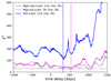 |
Fig. 4. χ2 value as a function of the time delay in the observer’s frame for the Mg II line emission (magenta line) as well as for the Fe II line emission (blue line). The global χ2 minima for each line are depicted by the vertical dashed lines. The χ2 time-delay dependence for the previous, shorter continuum-Mg II light curves (Czerny et al. 2019) is shown as a gray line with the global minimum at the time delay twice as large as for the current data. Cont:79, 113 and line:26, 35 represents the number of observations. |
The estimators of data regularity/randomness (von Neumann and Bartels) indicate the minimum estimator value for the time delay of ∼511 − 512 days in the observer’s frame for the Mg II line; see Table 4. Here, we inferred the peak and the mean time delays and the corresponding peak uncertainty based on 1000 bootstrap realizations for each estimator. Essentially the same best time-delay is also found for the Fe II line. However, the mean time-delay value for the Fe II line is lower than the mean value for the Mg II line, that is, 273.0 days versus 313.8 days for the von Neumann estimator and 289.3 days versus 339.1 days for the Bartels estimator. This lower value is caused by the secondary prominent minimum for the Fe II line, which is at ∼327 − 335 days for the von Neumann estimator and at ∼327 − 381 days for the Bartels estimator; see Fig. 5 (von Neumann estimator) and Fig. 6 (Bartels estimator).
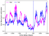 |
Fig. 5. Von Neumann estimator as a function of the time delay in the observer’s frame for the total Mg II (magenta line) and Fe II (blue line) emissions. The dashed vertical line marks the common global minimum of the von Neumann estimator at ∼512.0 days. |
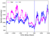 |
Fig. 6. Bartels estimator as a function of the time delay in the observer’s frame for the total Mg II (magenta line) and Fe II (blue line) emissions. The dashed vertical line marks the common global minimum of the Bartels estimator at ∼512.0 days. |
The analysis performed using the discrete correlation function (DCF) indicates a global peak at 527.5 days for the total Mg II and Fe II emission light curves (specifically for the slot weighting of light curve pairs with a time step of 5 days). When we constructed 400 bootstrap realizations of continuum–line emission pairs, we obtained a peak time delay of  days for the Mg II total emission and
  days for the Fe II total emission, thatis, the time delay appears to be the same within the uncertainties for both lines. However, the overall time-delay peak distribution is broad with multiple peaks.
The time-delay analysis using the z-transformed discrete correlation function (zDCF) yields peak values with large uncertainties, especially for the Mg II emission, for which we obtained  days in the observer’s frame. For the Mg II emission, the peak time delay is smaller than the peak time delay for the Fe II emission, for which we obtained
  days. The zDCF value as a function of the time delay is depicted in Fig. 7 for both lines. The zDCF time-delay peak for the Mg II line is broader and has a smaller correlation coefficient of
  than the one for the Fe II line,
  .
.
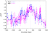 |
Fig. 7. zDCF correlation coefficient as a function of the time delay in the observer’s frame for the total Fe II (blue line) and the total Mg II emission (magenta line). The vertical lines denote the peak values for each corresponding line. |
In summary, using different time-delay determination methods, we consistently detect a time-delay peak close to ∼520 days for the Mg II emission in the observer’s frame, while for the total Fe II emission, we detect two time delays, at ∼340 days and ∼510 days, both of which are usually present in the time-delay distributions. Two peaks of comparable height have occasionally been reported for other lines such as Hβ (Du et al. 2015). When we add comparable time-delay peaks, we obtain a mean time delay of  days for the Mg II emission and
  and
and  days for the Fe II emission. When calculated with respect to the rest frame of the source at the redshift of z = 0.90052, the total Mg II emission time delay is
  days. For the total Fe II emission, the longer rest-frame time delay is
  days, which is consistent with the Mg II time delay within the uncertainties. The shorter Fe II rest-frame time delay is
  days. The light-travel distance of the Mg II emission region is 0.23 pc. For the Fe II region, the setup is more complex. Its mean distance is comparable to the Mg II emission region, ∼0.23 pc, based on the longer time-delay peak. However, the shorter time-delay indicates that the Fe II region is more extended in the direction toward the observer, as we discuss further in Sect. 5. Due to the nonzero inclination, a part of the Fe II region is located by (275.5 − 180.3)c ∼ 0.08 pc closer to the observer. When illuminated by the same photoionizing radiation, a fraction of the Fe II-reprocessed photons reaches the observer sooner than the Mg II-reprocessed radiation, while the other part shares the same reprocessing region with Mg II.
We stress that the two possible solutions (two time delays) for the Fe II emission are clearly detected only with the χ2 method. We list two time delays for Fe II line because some methods indicate a time-delay peak close to ∼500 days in the observer’s frame (JAVELIN, von Neumann, Bartels, DCF), while the rest detected the peak close to ∼350 days (ICCF, χ2, zDCF). In addition, from the distribution of time-delay minima and peaks, we detect consistently lower mean and median values for the Fe II complex (von Neumann, Bartels, χ2), which implies that the geometrical structure of the Fe II broad-line pseudo-continuum is complex. Longer and denser light curves would help to further disentangle Mg II and Fe II time delays.
To assess how the time-delay analysis depends on outliers, we identified four data points in the Mg II and the Fe II flux densities, see Table 2, which appear to be outliers. These are measurements 9, 17, 18, and 26. After these points were removed, the time-delay peak and centroid values for the Mg II and the Fe II lines were not significantly modified with respect to the original light curves; see Table 4. However, quite interestingly, the difference between the Mg II and the Fe II time delays persisted, in particular, the trend that the Fe II line has a shorter time delay than the Mg II line for more time-delay determination methods. See Appendix B for a detailed analysis and description.
4.3. Wavelength-resolved time lags
As discussed in Sect. 3.3, seven light curves were created from the different parts of the RMS spectrum. The lighcurves are shown in Fig. 8. The original curves were properly normalized, but for a better comparison with photometry they are also plotted in magnitude scale, with arbitrary normalization.
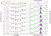 |
Fig. 8. First column: continuum light curve in magnitude (first panel) and the seven curves in different wavebands derived from the combination of photometric and the spectroscopic observations (remaining panels). The corresponding waveband ranges are listed in Table 3. Curves 1 and 7 are in unit of 10−17 and other curves are in 10−16. Second column: auto-correlation of continuum and the ICCF results for all the curves with respect to continuum. Histograms are the peak (red) and centroid (blue) distribution from the ICCF with 10 000 bootstrap realizations. |
To understand the kinematics and the geometry of broad line region (BLR) in quasars, velocity-resolved time lags are essential. Here we present our investigation of BLR kinematics in the bright quasar CTS C30.10 using its Mg II+Fe II emission, with the continuum power-law subtracted. The Mg II+Fe II combination was divided into seven different velocity bins after the continuum power-law was subtracted. The corresponding seven light curves were produced, and the time delay with respect to the V-band continuum light curve was finally investigated using different methods. The methods described in Appendix A.1 were used to estimate the time lags (and the uncertainty) between the various curves and the continuum. The results are summarized in Table 5.
Time-delay measurements for seven wavelength bins containing a combination of Mg II and Fe II emission, after subtracting the power-law component.
ICCF: the interpolated cross-correlation function (ICCF) is shown for each light curve in Fig. 9 (left panel). According to the time-delay values inferred from the maximum correlation coefficient, see Table 5, the time delay is between 340 and 380 days in the observer’s frame, with a weak increase for light curves 4, 5, and 6. The maximum correlation coefficient is ∼0.6 − 0.7. The ICCF uses the flux and amplitude randomization technique to estimate the time lag distribution, in particular, its centroid and the peak. We estimated the centroid and the peak time lag, and corresponding plots are shown in Fig. 8. For all the curves, the time lags from the centroid are consistent within the error bars between ∼330–370 days. However, the time lags from the peak distribution are higher in all the curves than centroid values, and lie between ∼340–385 days. In both cases, the longer time lags are noted in curves 4, 5, and 6, which is expected as they represent the Mg II part of the spectrum.
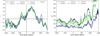 |
Fig. 9. ICCF and χ2 values as a function of time delay. Left panel: ICCF as a function of time delay (expressed in days in the observer’s frame) for the seven light curves according to the legend. Right panel: χ2 value as a function of the time delay (in days) in the observer’s frame for the seven light curves according to the legend. |
χ2: this method is based on the χ2-minimization technique. The results obtained from this method are generally consistent with the ICCF results. The time delays were found to be between ∼324–538 days, with longer time delays for light curves 4, 5, and 6. The χ2 values as a function of time delay for individual light curves are shown in Fig. 9 (right panel). The longer time delays are consistent with the RMS spectrum shown in Fig. 10, where curves 4 and 5 lie exactly in the middle of the Mg II line emission. The bootstrap technique was also applied to obtain the time-delay peak distribution. We generated 10 000 light-curve pairs based on the actual seven light curves. Based on the time-delay peak distribution, we determined the final peak and the mean of the distribution. The final peak asymmetric error bars were inferred from the left and right standard deviations within 30% of the main peak surroundings. The mean time-delay follows a similar trend of increasing and decreasing time delays toward longer wavelengths, with the longest time delay of 558.3 days for light curve 4.
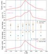 |
Fig. 10. Wavelength-dependent time lags from various methods along with the mean and RMS spectrum. Time lags seem to weakly follow the RMS spectrum. |
Data regularity estimators (von Neumann, Bartels): when we applied the data regularity estimators (von Neumann, Bartels) to the seven light curves, we obtained a minimum estimator value at ∼512 days in the observer’s frame for the von Neumann and Bartels estimators; see Table 5 and Fig. 11. However, the estimator profile as a function of the time delay changes qualitatively close to this global minimum. Closer to the Mg II line wings, the broad minimum is shallower; see Fig. 11 for the von-Neumann estimator (left panel) and the Bartels estimator (right panel). This also results in the lower mean value of the peak time delay as inferred from the bootstrap analysis (1000 realizations). This is in contrast to light curves 3, 4, and 5 close to the line center, where the minimum at ∼512 days is more pronounced, resulting in higher mean time-delay values.
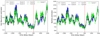 |
Fig. 11. Estimators of data randomness/regularity as a function of the time delay in the observer’s frame. Left panel: von Neumann estimator for seven Mg II line light curves according to the legend. Right panel: Bartels estimator value for the same Mg II light curves in the observer’s frame. The dashed red line represents the estimated time delay. |
DCF: investigating the time lags using the DCF method yielded shorter time lags for all the seven light curves than with the other methods. The dominant peak in the observer’s frame is at 187.5 days both for the default DCF investigation using the observed light curves and in the peak distribution inferred from 200 bootstrap realizations for each light curve. In Table 5 we separately list the peak values for the DCF evaluation using the slot- and the Gauss-weighting of the light-curve pairs, where the time bin is constant and we set it to 25 days. For the bootstrap runs, we separately calculated the peak and the mean values of the corresponding time-lag peak distributions. While the peak is always close to 187.5 days, the mean value shifts toward higher values for light curves 4 and 5 because the secondary time-lag peak at ∼450 − 550 days becomes more prominent for these light curves.
zDCF: for the zDCF method, the measured time delays agree within the uncertainties. The peak values of the time delay are 327.9 days in the observer’s frame for the first three wavebands, then they increase to 370.5 days for bands 4, 5, and 6. The emission light curve 7, corresponding to the red wing of the line, has the peak time delay again at 327.9 days. The zDCF values as a function of the time delay in the observer’s frame are depicted in Fig. 12 for individual light curves, and the results are presented in Table 5. The shift of 42.6 days between the time-delay peaks of the first (and the second, third, and seventh light curves) and the fifth light curve (and the fourth and sixth light curves) is highlighted by the corresponding horizontal lines.
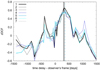 |
Fig. 12. z-transformed DCF as a function of the time delay in the observer’s frame for individual light curves according to the legend. Overall, there is a time-delay peak between 300 and 400 days, consistent within the uncertainties for all the light curves. We highlight the shift of ∼40 days between the time-delay peaks of the first and fifth waveband by using the corresponding horizontal lines to denote the peak values. |
JAVELIN: the results from JAVELIN are shown in Fig. 13. The recovered time delays are much higher than with the ICCF. For most of the curves (curves 1, 3, 4, 5, 6 and 7), the recovered time delays are between ∼502–529 days. For curve 2, we found rather a short time delay of about 195 days, also much shorter than with the ICCF. To quantify the error bars on the time-delay results, we applied the bootstrap technique for 1000 realizations and estimated the peak time delay with 1σ error bar. The results are presented in Table 5. Time delays corresponding to various curves are shown with the RMS spectrum in Fig. 10, and they agree with the χ2 method for most of the curves.
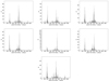 |
Fig. 13. Javelin bootstrap results with 1000 realizations for all the seven curves (from left to right). The peak and results from this are listed in Table 4. |
4.4. Summary of the wavelength-dependent trends and BLR kinematics
The visual summary of the observed trends is given in Fig. 10. The time delays in curves dominated by the Mg II emission are longer than for Fe II-dominated curves, specifically, 1 or 7. The two-component character of Mg II line is not detected. Component 1 dominated curve 4 and component 2 dominates curve 5, but there is no differences between the time delays for these two curves. This supports the conclusion that the need for two components rather reflects a more complex line shape than the actual existence of the two physically separated regions, as was already argued by Modzelewska et al. (2014) on the basis of the mass measurement consistency. Some level of asymmetry of the Mg II line is frequently seen, and two-component fits are required (Marziani et al. 2013), but these authors showed that nevertheless, Mg II is a better virial indicator of the BLR motion than Hβ because the centroid shifts with respect to the rest frame are lower.
Our wavelength-resolved data contain no clear anisotropy in the line shape, the time delay neither decreases or increases systematically with the wavelength. This means that we do not detect traces of an inflow or outflow. We did not attempt to study the Mg II shape separately because subtracting Fe II would lead to large errors in the line wings, Therefore we did not expect any new results from such an approach with the current data set.
5. Discussion
We determined the time delay of the Mg II emission and Fe II emission with respect to the continuum in quasar CTS C30.10 (z = 0.90052). While the Mg II time delay has been determined before for several sources (see Khadka et al. 2021 for a current list of sources), Fe II time delays in the UV have not been generally measured. So far, the UV Fe II time delay was reported only for NGC 5548, and Maoz et al. (1993) found a similar time lag for UV Fe II lines as for Lyα.
Using several methods, we determined the Mg II time delay at  days in the observed frame. The time delay for Fe II was not unique, and two values are favored:
  and
and  days. This likely suggests a more complex reprocessing region. In some cases, it is clear that Fe II has more than one component and is well fit with two components (Dong et al. 2010, Hryniewicz et al. 2022).
The time delays for Fe II seem to be 10% shorter on aberage than for Mg II for a given method, and much shorter time delays are indicated. This is rather unexpected on the basis of the kinematic line width. The Fe II template used in the spectral fitting was broadened to a full width at half maximum (FWHM) = 2115 km s−1, This broadening was adjusted on the basis of χ2 optimization by Modzelewska et al. (2014), and was also tested with the current data. The Mg II line was fit as a two-component line, and the mean value of the FWHM of component 1 is 2756 ± 122 km s−1, for component 2, it is 3558 ± 102 km s−1, and if the line is treated as a single-component line of more complex shape, the total FWHM is 4868 ± 114 km s−1. Therefore, the line width implies that the Fe II is located farther out than Mg II, consistent with the lower ionization potential for Fe II.
Therefore we also used a wavelength-resolved approach to a signal containing both Mg II and Fe II, with the aim to shed more light onto the relative geometry of the two regions. The data quality is not excellent, but we see a similar overall trend as for the Mg II and Fe II light curves. In Tables 4 and 5 we give the results for the peak as well as median values for a given method. In the case of ICCF, the discussion by Koratkar & Gaskell (1991) shows that the centroid-based values correspond to the luminosity-weighted radius, while peak values are more affected by the gas at small radii. However, our ICCF-based results do not show significant differences there, being consistent rather with a relatively compact reprocessing region.
To independently test the extension of the emitting regions, we calculated the auto-correlation function (ACF) of total Mg II and Fe II along with the continuum. The result is show in Fig. 14. The ACF of continuum decays at timescales of 250 days. The secondary peak reappears on a timescale of 750 days. In their central parts, the ACF of Fe II is broader than that of Mg II, suggesting a more extended emission region for Fe II. However, both functions show a plateau on timescales 200–500 days, which is not a typical feature of AGN light curves. All these unexpected effects are likely connected to the apparent similarity of the two peaks in the continuum light curve, separated by ∼1500 days. In a still longer data sequence, this apparent similarity would likely disappear.
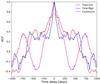 |
Fig. 14. Auto-correlation function of total Mg II and total Fe II along with the continuum. |
The Mg II and Fe II emission regions are extended, however, and the apparent discrepancy between the narrower Fe II lines but shorter effective Fe II delay can be solved, as illustrated in Fig. 15. If the observer is inclined with respect to the symmetry axis, there is a clear asymmetry in the visibility of the BLR part closer to the observer and the part located at the far side of the black hole. The region emitting mostly Mg II can still be transparent for the continuum, so Fe II is produced, but the Fe II emitting region can partially suppress the Mg II emission from the near side. The opposite can happen for the far side: now the Mg II emitting region is much better exposed while Fe II is partially shielded. Because the measured time delay is the weighted average over the entire region, the net Fe II time delay can still be shorter because the closest part dominates more.
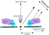 |
Fig. 15. Schematic representation of the Mg II and Fe II emission regions. The mean distance of the Mg II and Fe II region from the BH is ∼0.23 pc, estimated from the rest frame time delays, 276 days and 270 days for Mg II and Fe II, respectively. The Fe II emission also exhibits a shorter time delay in the rest frame, 180 days, which indicates the larger extent of the Fe II region with respect to the Mg II emission region in the direction away from the SMBH. Hence, due to a non-negligible inclination of the observer, the reprocessed emission from the Fe II region finally tends to come to the observer sooner. The secondary time delays at ∼570 and ∼680 days can potentially be attributed to the mirror-effect, i.e., the Mg II and Fe II emission, respectively, coming to the observer from the other side of the accretion disc, which is supported by the temporal difference of (570 − 270) = 300 days, which corresponds to ∼0.25 pc, i.e., one additional disk crossing of photons. However, the Fe II emission coming from the more distant part across the disk is partially shielded by the Mg II line-emitting region closer in with respect to the observer. Color does not represent the density of the cloud. |
5.1. BLR kinematics
The wavelength-resolved or velocity-resolved time lags allow us to explore the BLR geometry and kinematics. The distribution of estimated time lags with corresponding wavelength can have different shapes, namely, a symmetric shape suggesting Keplerian or disk-like rotation of the BLR. Results obtained by other authors for the Hβ line, which also belongs to low ionization lines, are different, as for Mg II and Fe II. Grier et al. (2017) did not claim any outflows/inflows based on their study of four sources, although they required elliptical orbits.
Velocity-resolved reverberation mapping of 3C120, Ark120, Mrk 6, and SBS 1518+593 was reported by Du et al. (2018a). Their results show that the first three AGN have complex features that are different from the simple signatures expected for pure outflows, inflow, or a Keplerian disk. Moreover, SBS 1518+593 shows the least asymmetric velocity-resolved time lags characteristic of a Keplerian disk. They also observed a significant change in the velocity-resolved time lags of 3C 120 compared to its previous study, suggesting an evolution of the BLR structure. Hu et al. (2020) have studied the quasar PG 0026+129, and their results show evidence of two distinct BLRs. Their velocity-resolved analysis supports two regions, but does not imply any simple inflow/outflow pattern. Lu et al. (2016) provided a detailed study of reverberation mapping of the BLR in NGC 5548. Their velocity-binned delay map for the broad Hβ line shows a symmetric response pattern around the line center. They suggested that it might be a plausible kinematic signature of virialized motion of the BLR. Another study of NGC 5548 by Pei et al. (2017) found a complex velocity-lag structure with shorter lags in the line wings of Hβ. They concluded again that the BLR is dominated by Keplerian motion. The same conclusion was reached by Xiao et al. (2018) for the same source.
Recently, Vivian et al. (2022) have reported velocity-resolved Hβ time lags for several nearby bright Seyfert galaxies in which they observed all possible scenarios, including Keplerian motion of the BLR and radially in-falling and out-flowing materials. A study of the high-ionization line velocity structure (CIV) in NGC 5548 was reported by De Rosa et al. (2015), with a six-month-long observation taken from Cosmic Origins Spectrograph on the Hubble Space Telescope. They observed a significant correlated variability in the continuum and the broad emission lines. Their velocity-resolved time lag study shows coherent structure in lag versus line-of-sight velocity for the emission lines, but they detected no clear outflow signatures. This could be related to a relatively low Eddington ratio in this source, and no clear shift in CIV, frequently seen in quasars.
Our data show no monotonic increase or decrease of the time delay with wavelength, which is the signature of inflow or outflow. Thus the dynamics in CTS C30.10 seems to be consistent with predominantly Keplerian motion. Time delays measured in a wavelength-dependent way for a combination of Mg II and Fe II as well as separate time-delay measurement for the total Mg II and Fe II emission, combined with the kinematic line width, imply a stratification in the BLR, but also a clear asymmetry in the visibility of the BLR part closer to the observer and the part that is more distant, as visualized in Fig. 15.
5.2. Updated Mg II radius-luminosity relation
Following our previous constructions of the Mg II-based radius-luminosity (RL) relation (Czerny et al. 2019; Zajaček et al. 2020, 2021; Martínez-Aldama et al. 2020b; Khadka et al. 2021), we updated this relation for 78 available reverberation-mapped sources, including the updated rest-frame time delay of the total Mg II emission for CTS C30.10,  days; see Figs. 16 and 17. The RL relation is generally well defined with a significant positive correlation between the rest-frame Mg II time delay and the monochromatic luminosity at 3000 Å. The Spearman correlation coefficient is s = 0.49 (p = 4.96 × 10⁻⁶) and the Pearson correlation coefficient is r = 0.63 (p = 8.39 × 10⁻¹⁰), which motivates the search for a power-law relation of the form τ = KLα.
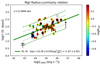 |
Fig. 16. Radius-luminosity relation for the currently available 78 Mg II sources. The best-fit relation determined by the classical least-squares fitting is indicated by the solid green line. The updated Mg II emission-line time delay of |

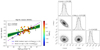 |
Fig. 17. Mg II maximum likelihood RL relation determined using the MCMC algorithm (left panel). The coefficients as well as the RMS scatter are consistent within the uncertainties with the classical fitting algorithm (see Fig. 16). CTS C30.10 is depicted using the black circle, while the previous time-delay measurement, approximately twice as long, is represented by a gray circle. The dashed violet line shows the Bentz RL relation with a slope of ∼0.5, which was adjusted for the continuum luminosity at 3000 Å. Right panel: corner plot representation of the distribution histograms for the two parameters α (slope) and K constant in the linear fit of logτ = α log L44 + K to the Mg II data. The likelihood function is included the underestimation factor f, whose distribution is also shown. |
We fit the linear function logτ = αlog(L3000/1044 erg s−1) + K to the 78 Mg II data using the classical least-square fitting procedure as well as the Monte Carlo Markov chain algorithm. From the least-squares fitting, we obtain the best-fit radius-luminosity relation
 (5)
(5)
with a scatter of σ = 0.29 dex. The best-fit relation is depicted in Fig. 16 along with 78 RM sources, 66 of which are color-coded according to the relative Fe II strength, RFe II, which serves as a suitable observational proxy for the accretion-rate intensity (Martínez-Aldama et al. 2020b).
Using the MCMC algorithm, including the uncertainty underestimation factor f, we obtain the maximum-likelihood RL relation,
 (6)
(6)
with a scatter of σ ≃ 0.29 dex. The RMS scatter as well as the inferred RL relation are consistent within the uncertainties with the values determined from the least-squares fitting. The maximum likelihood relation is shown along with the Mg II data in Fig. 17 (left panel) alongside the corner plot (right panel) with the slope and the intercept distributions. The new shorter Mg II time delay (depicted by a black circle in Figs. 16 and 17) now lies within the 2σ prediction interval of the whole sample, see Fig. 16, while previously, it was within the 1σ interval. For the MCMC fitting, the new Mg II time delay also lies within 2σ of the median RL relation.
In addition, we also considered for comparison the former RL relation based on the reverberation-mapped Hβ sample (Bentz et al. 2013). The Bentz relation has a slope of ∼0.5, that is, it is consistent with the simple photoionization theory. We transformed the Bentz relation inferred for the monochromatic luminosity at 5100 Å to the RL relation for 3000 Å and obtained logτ = 1.391 + 0.533log(L3000/1044 erg s−1), that is, the same slope, but a slightly smaller intercept (Zajaček et al. 2020). Interestingly, the shorter time delay of CTS C30.10 is now consistent with this relation; see Fig. 17 (left panel). However, the RMS scatter of the whole Mg II sample along the Bentz relation is larger (σ ∼ 0.35 dex) than the maximum-likelihood RL relation (σ ∼ 0.29 dex).
Du & Wang (2019) investigated the extended RL relations using the relative Fe II strength with respect to the Hβ line, RFe II = EW(Fe II)/EW(Hβ). The idea was to decrease the scatter in Hβ sources along the RL relation, which appears to be driven by the accretion-rate intensity. Because RFe II is correlated with the accretion rate, it should provide the correction. A certain improvement was reported with a final scatter of 0.196 dex in comparison with the original Hβ RL relation with σ ∼ 0.28 dex (Du et al. 2018b).
In our case, the relative strength is defined analogously as the ratio of the equivalent width of Fe II to the equivalent width of Mg II, RFe II = EW(Fe II)/EW(Mg II). Hence, we investigate analogously to Du & Wang (2019) the extended RL relation in the form log τ = α log(L3000/1044erg s−1) + β log RFe II + K. The correlation between the rest-frame time delay logτ and the term log L44 + β/α log RFe II2 is weaker than for the simple RL relation, but still present, with a Spearman correlation coefficient of s = 0.39 (p = 0.0013) and a Pearson correlation coefficient of r = 0.52 (p = 6.16 × 10⁻⁶).
In Fig. 18 (left panel), we show the extended RL relation for 66 sources with available RFe II measurements, with an updated time-delay of CTS C30.10,  days, including the median RL relation inferred using the MCMC method as well as the distribution of 1000 randomly selected relations. In the right panel of Fig. 18, we display the corner plot representation of parameter distributions. Maximizing the likelihood function leads to the following parameter inferences:
  ,
,  , and
, and  . The underestimation factor is
  . The RMS scatter is 0.28 dex, which is a decrease by only 3.7% with respect to a simple RL relation with a scatter of 0.29 dex (displayed in Fig. 17). Hence, we cannot confirm a significant decrease in the scatter for Mg II sources for the extended RL relation. However, splitting the source sample into high and low accretors can lead to a significant scatter decrease, at least for the current sample of RM Mg II quasars, which was analyzed by Martínez-Aldama et al. (2020b).
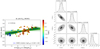 |
Fig. 18. Extended RL relation including the relative Fe II strength, RFe II. Left panel: median relation (blue line) is inferred by maximizing the likelihood function. Green lines show 1000 random selections from the parameter distribution. 66 Mg II time-delay measurements are color-coded to depict log RFe III according to the color axis on the right. The RMS scatter is 0.28 dex. Right panel: corner plot shows the parameter distributions inferred from the MCMC method. The parameter uncertainties correspond to 16th and 84th percentiles. |
5.3. UV Fe II RL relation
Previously, only one measurement of the UV Fe II pseudo-continuum was performed for the Seyfert galaxy NGC 5548 during the campaign in 1988–1989 with IUE satellite (Maoz et al. 1993). The Fe II time-delay centroid was inferred to be  days. The corresponding monochromatic luminosity at 3000 Å for this source is log[L3000(erg s−1)] = 43.696 ± 0.051 according to the NED database3, which was inferred considering the flux densities determined close to 3000 Å.
Here we report two potential time-delay peaks for the UV Fe II pseudo-continuum for the more luminous source CTS C30.10,  days and
  days. The monochromatic luminosity for the source is log[L3000(erg s−1)] = 46.023 ± 0.026. Because the UV Fe II RL relation has not been investigated before, the two measurements across three orders of magnitude in luminosity now allow us to preliminarily discuss its existence for the first time.
In Fig. 19, the preliminary UV Fe II radius-luminosity relation is outlined, which confirms the basic trend and the power-law dependence with the slope close to 0.5. Using the shorter Fe II time delay of 180.3 days for CTS C30.10 yields the relation logτ = (0.54 ± 0.04) log L44 + (1.16 ± 0.08), while the longer time delay of 270.0 days leads to logτ = (0.62 ± 0.03) log L44 + (1.19 ± 0.06). The uncertainties were calculated by the propagation of errors of the time delays and the luminosities of the two sources. The longer time delay for Fe II is more consistent with the RL relation of Bentz et al. (2013) when renormalized for the monochromatic luminosity at 3000 Å. This agrees with the picture sketched in Fig. 15, where the Mg II and Fe II line-emitting regions share approximately the common mean distance from the SMBH corresponding to ∼270 − 275.5 days. The Fe II emitting region is, however, more extended towards larger distances from the SMBH, with one side closer to the observer, which effectively produces the second, shorter time-delay peak.
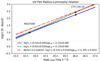 |
Fig. 19. Preliminary RL relation for the UV Fe II pseudo-continuum based on the two time-lag measurements for NGC 5548 (Maoz et al. 1993) and CTS C30.10 (this work). We derive two relations based on the two Fe II time delays for CTS C30.10: 180.3 days and 270.0 days. The longer time delay of 270.0 days is more consistent with the RL relation derived by Bentz et al. (2013) when renormalized to the 3000 Å monochromatic luminosity. The shaded regions depict 1σ confidence intervals of individual RL relations. |
6. Conclusions
We summarize the main results of nine years of monitoring the luminous quasar CTS C30.10 (2012–2021) below.
-
The Mg II line emission exhibits a rest-frame time delay of
 days, which is about a factor of two shorter than the previously reported value for this source. This shows that the duration of the monitoring is essential to accurately determine the emission-line time delay, especially if more time-delay peaks are present.
 -
The Mg II time-delay is consistent within 2σ with the best-fit RL relation for all current RM Mg II quasars. It also lies on the previously determined Hβ RL relation with a slope close to 0.5.
-
The rest-frame time delay for the Fe II emission has two components:
 days and
  days. Because the Fe II line width is smaller than that of the Mg II line, it is expected to be located farther from the SMBH. On the other hand, the mean distance of the emission regions is comparable, as is indicated by the common time-delay component within the uncertainties. The shorter time-delay component indicates that the observer predominantly sees the Fe II emission region oriented toward them, while the more distant region is mostly shielded by the closer Mg II region.
 -
Combining our UV Fe II time-delay measurement with the older one in NGC 5548, we find that these measurements indicate the existence of the UV Fe II RL relation, whose slope is consistent with 0.5 within the uncertainties. The longer Fe II time delay is consistent with the Hβ RL relation, which indicates that a time delay of ∼270 days expresses the mean distance of the Fe II region, while a shorter time delay of ∼180 days is associated with the extension of Fe II region closer to the observer and away from the SMBH.
-
The wavelength-resolved reverberation mapping of the Mg II+Fe II complex between 2700 and 2900 Å shows that this region is stratified with the core of the Mg II emission line having a longer time delay than the wings dominated by Fe II. This reflects the geometrical orientation of this complex with respect to the observer.
We will continue to monitor this source and few more luminous quasars with SALT, and hope to create better RL relation for Fe II.
L44 ≡ L3000/(1044 erg s−1).
Acknowledgments
This paper uses observations made at the South African Astronomical Observatory (SAAO). The project is based on observations made with the SALT under programs 2012-2-POL-003, 2013-1-POL-RSA- 002, 2013-2-POL-RSA-001, 2014-1-POL-RSA-001, 2014-2-SCI-004, 2015-1-SCI-006, 2015-2-SCI-017, 2016-1-SCI-011, 2016-2-SCI-024, 2017-1-SCI-009, 2017-2-SCI-033, 2018-1-MLT-004 (PI: B. Czerny). The project was partially supported by the Polish Funding Agency National Science Centre, project 2017/26/A/ST9/00756 (MAESTRO 9), and MNiSW grant DIR/WK/2018/12. Some of the observations reported in this paper were obtained with the Southern African Large Telescope (SALT). Polish participation in SALT is funded by grant No. MNiSW DIR/WK/2016/07. The authors also acknowledge the Czech-Polish mobility program (MŠMT 8J20PL037 and NAWA PPN/BCZ/2019/1/00069). MZ acknowledges the financial support of the GAČR EXPRO grant No. 21-13491X “Exploring the Hot Universe and Understanding Cosmic Feedback”. SP acknowledges financial support from the Conselho Nacional de Desenvolvimento Científico e Tecnológico (CNPq) Fellowship (164753/2020-6). MLM-A acknowledges financial support from Millenium Nucleus NCN19_058 (TITANs).
References
- Alexander, T. 1997, in Astronomical Time Series, eds. D. Maoz, A. Sternberg, & E. M. Leibowitz, Astrophysics and Space Science Library, 218, 163 [Google Scholar]
- Antonucci, R. 1993, ARA&A, 31, 473 [Google Scholar]
- Antonucci, R. R. J., & Miller, J. S. 1985, ApJ, 297, 621 [NASA ADS] [CrossRef] [Google Scholar]
- Barth, A. J., Pancoast, A., Bennert, V. N., et al. 2013, ApJ, 769, 128 [NASA ADS] [CrossRef] [Google Scholar]
- Bentz, M. C., Horne, K., Barth, A. J., et al. 2010, ApJ, 720, L46 [NASA ADS] [CrossRef] [Google Scholar]
- Bentz, M. C., Denney, K. D., Grier, C. J., et al. 2013, ApJ, 767, 149 [Google Scholar]
- Bian, W.-H., Huang, K., Hu, C., et al. 2010, ApJ, 718, 460 [NASA ADS] [CrossRef] [Google Scholar]
- Blandford, R. D., & McKee, C. F. 1982, ApJ, 255, 419 [Google Scholar]
- Boehle, A., Ghez, A. M., Schödel, R., et al. 2016, ApJ, 830, 17 [Google Scholar]
- Boroson, T. A., & Green, R. F. 1992, ApJS, 80, 109 [Google Scholar]
- Bruhweiler, F., & Verner, E. 2008, ApJ, 675, 83 [NASA ADS] [CrossRef] [Google Scholar]
- Cackett, E. M., Bentz, M. C., & Kara, E. 2021, Iscience, 24, 102557 [NASA ADS] [CrossRef] [Google Scholar]
- Chelouche, D., Pozo-Nuñez, F., & Zucker, S. 2017, ApJ, 844, 146 [CrossRef] [Google Scholar]
- Crawford, S. M., Still, M., Schellart, P., et al. 2010, in Observatory Operations: Strategies, Processes, and Systems III, eds. D. R. Silva, A. B. Peck, B. T. Soifer, et al., SPIE Conf. Ser., 7737, 773725 [NASA ADS] [CrossRef] [Google Scholar]
- Czerny, B., Hryniewicz, K., Maity, I., et al. 2013, A&A, 556, A97 [NASA ADS] [CrossRef] [EDP Sciences] [Google Scholar]
- Czerny, B., Olejak, A., Rałowski, M., et al. 2019, ApJ, 880, 46 [Google Scholar]
- Czerny, B., Martínez-Aldama, M. L., Wojtkowska, G., et al. 2021, Acta Phys. Pol. A, 139, 389 [NASA ADS] [CrossRef] [Google Scholar]
- De Rosa, G., Peterson, B. M., Ely, J., et al. 2015, ApJ, 806, 128 [NASA ADS] [CrossRef] [Google Scholar]
- De Rosa, G., Fausnaugh, M. M., Grier, C. J., et al. 2018, ApJ, 866, 133 [NASA ADS] [CrossRef] [Google Scholar]
- Denney, K. D., Peterson, B. M., Pogge, R. W., et al. 2010, ApJ, 721, 715 [NASA ADS] [CrossRef] [Google Scholar]
- Done, C., & Krolik, J. H. 1996, ApJ, 463, 144 [NASA ADS] [CrossRef] [Google Scholar]
- Dong, X.-B., Ho, L. C., Wang, J.-G., et al. 2010, ApJ, 721, L143 [NASA ADS] [CrossRef] [Google Scholar]
- D’Onofrio, M., Marziani, P., Sulentic, J. W., et al. 2012, in Fifty Years of Quasars: From Early Observations and Ideas to Future Research, eds. M. D’Onofrio, P. Marziani, J. W. Sulentic, et al., Astrophysics and Space Science Library, 386, 11 [CrossRef] [Google Scholar]
- Du, P., & Wang, J.-M. 2019, ApJ, 886, 42 [NASA ADS] [CrossRef] [Google Scholar]
- Du, P., Hu, C., Lu, K.-X., et al. 2015, ApJ, 806, 22 [NASA ADS] [CrossRef] [Google Scholar]
- Du, P., Brotherton, M. S., Wang, K., et al. 2018a, ApJ, 869, 142 [CrossRef] [Google Scholar]
- Du, P., Zhang, Z.-X., Wang, K., et al. 2018b, ApJ, 856, 6 [NASA ADS] [CrossRef] [Google Scholar]
- Eckart, A., Hüttemann, A., Kiefer, C., et al. 2017, Found. Phys., 47, 553 [NASA ADS] [CrossRef] [Google Scholar]
- Edelson, R. A., & Krolik, J. H. 1988, ApJ, 333, 646 [Google Scholar]
- Edelson, R., Turner, T. J., Pounds, K., et al. 2002, ApJ, 568, 610 [CrossRef] [Google Scholar]
- EHT Collaboration (Akiyama, K., et al.) 2019a, ApJ, 875, L1 [Google Scholar]
- EHT Collaboration (Akiyama, K., et al.) 2019b, ApJ, 875, L4 [Google Scholar]
- Gaskell, C. M. 2009, New A Rev., 53, 140 [NASA ADS] [CrossRef] [Google Scholar]
- Gaskell, C. M., & Peterson, B. M. 1987, ApJS, 65, 1 [NASA ADS] [CrossRef] [Google Scholar]
- Gaskell, C. M., Bartel, K., Deffner, J. N., & Xia, I. 2021, MNRAS, 508, 6077 [NASA ADS] [CrossRef] [Google Scholar]
- Gillessen, S., Plewa, P. M., Eisenhauer, F., et al. 2017, ApJ, 837, 30 [Google Scholar]
- Goad, M. R., Korista, K. T., Rosa, G. D., et al. 2016, ApJ, 824, 11 [NASA ADS] [CrossRef] [Google Scholar]
- GRAVITY Collaboration (Abuter, R., et al.) 2018a, A&A, 615, L15 [NASA ADS] [CrossRef] [EDP Sciences] [Google Scholar]
- GRAVITY Collaboration (Sturm, E., et al.) 2018b, Nature, 563, 657 [Google Scholar]
- GRAVITY Collaboration (Abuter, R., et al.) 2019, The Messenger, 178, 20 [NASA ADS] [Google Scholar]
- GRAVITY Collaboration (Abuter, R., et al.) 2020a, A&A, 636, L5 [NASA ADS] [CrossRef] [EDP Sciences] [Google Scholar]
- GRAVITY Collaboration (Amorim, A., et al.) 2020b, A&A, 643, A154 [NASA ADS] [CrossRef] [EDP Sciences] [Google Scholar]
- GRAVITY Collaboration (Amorim, A., et al.) 2021, A&A, 648, A117 [NASA ADS] [CrossRef] [EDP Sciences] [Google Scholar]
- Grier, C. J., Peterson, B. M., Pogge, R. W., et al. 2012, ApJ, 755, 60 [NASA ADS] [CrossRef] [Google Scholar]
- Grier, C. J., Pancoast, A., Barth, A. J., et al. 2017, ApJ, 849, 146 [NASA ADS] [CrossRef] [Google Scholar]
- Grier, C. J., Shen, Y., Horne, K., et al. 2019, ApJ, 887, 38 [NASA ADS] [CrossRef] [Google Scholar]
- Haas, M., Chini, R., Ramolla, M., et al. 2011, A&A, 535, A73 [NASA ADS] [CrossRef] [EDP Sciences] [Google Scholar]
- Homayouni, Y., Trump, J. R., Grier, C. J., et al. 2020, ApJ, 901, 55 [Google Scholar]
- Hoormann, J. K., Martini, P., Davis, T. M., et al. 2019, MNRAS, 487, 3650 [NASA ADS] [CrossRef] [Google Scholar]
- Horne, K., De Rosa, G., Peterson, B. M., et al. 2021, ApJ, 907, 76 [Google Scholar]
- Hryniewicz, K., Bankowicz, M., Małek, K., Herzig, A., & Pollo, A. 2022, A&A, 660, A90 [NASA ADS] [CrossRef] [EDP Sciences] [Google Scholar]
- Hu, C., Du, P., Lu, K.-X., et al. 2015, ApJ, 804, 138 [Google Scholar]
- Hu, C., Li, S.-S., Guo, W.-J., et al. 2020, ApJ, 905, 75 [NASA ADS] [CrossRef] [Google Scholar]
- Karas, V., Svoboda, J., & Zajaček, M. 2021, in RAGtime: Workshops on Black Holes and Neutron Stars, E1 [Google Scholar]
- Karas, V., Zajaček, M., Kunneriath, D., & Dovčiak, M. 2022, Adv. Space Res., 69, 448 [NASA ADS] [CrossRef] [Google Scholar]
- Kaspi, S., Smith, P. S., Netzer, H., et al. 2000, ApJ, 533, 631 [Google Scholar]
- Kaspi, S., Brandt, W. N., Maoz, D., et al. 2021, ApJ, 915, 129 [NASA ADS] [CrossRef] [Google Scholar]
- Kelly, B. C., Bechtold, J., & Siemiginowska, A. 2009, ApJ, 698, 895 [Google Scholar]
- Khadka, N., Yu, Z., Zajaček, M., et al. 2021, MNRAS, 508, 4722 [NASA ADS] [CrossRef] [Google Scholar]
- Khadka, N., Martínez-Aldama, M. L., Zajaček, M., Czerny, B., & Ratra, B. 2022, MNRAS, 513, 1985 [NASA ADS] [CrossRef] [Google Scholar]
- Koratkar, A. P., & Gaskell, C. M. 1991, ApJS, 75, 719 [NASA ADS] [CrossRef] [Google Scholar]
- Kozłowski, S. 2016, ApJ, 826, 118 [CrossRef] [Google Scholar]
- Kozłowski, S., Kochanek, C. S., Udalski, A., et al. 2010, ApJ, 708, 927 [CrossRef] [Google Scholar]
- Krolik, J. H. 1999, Active Galactic Nuclei: From the Central Black Hole to the Galactic Environment (Princeton: Princeton University Press) [Google Scholar]
- Li, Y.-R., Wang, J.-M., Ho, L. C., Du, P., & Bai, J.-M. 2013, ApJ, 779, 110 [NASA ADS] [CrossRef] [Google Scholar]
- Lira, P., Kaspi, S., Netzer, H., et al. 2018, ApJ, 865, 56 [NASA ADS] [CrossRef] [Google Scholar]
- Liutyi, V. M., & Pronik, V. I. 1975, in Variable Stars and Stellar Evolution, eds. V. E. Sherwood, & L. Plaut, 67, 591 [NASA ADS] [CrossRef] [Google Scholar]
- Lu, K.-X., Du, P., Hu, C., et al. 2016, ApJ, 827, 118 [CrossRef] [Google Scholar]
- Maoz, D., Netzer, H., Leibowitz, E., et al. 1990, ApJ, 351, 75 [NASA ADS] [CrossRef] [Google Scholar]
- Maoz, D., Netzer, H., Peterson, B. M., et al. 1993, ApJ, 404, 576 [NASA ADS] [CrossRef] [Google Scholar]
- Martínez-Aldama, M. L., Czerny, B., Kawka, D., et al. 2019, ApJ, 883, 170 [CrossRef] [Google Scholar]
- Martínez-Aldama, M. L., Panda, S., Czerny, B., Zajacek, M., & LSST AGN SC Collaboration 2020a, in Multifrequency Behaviour of High Energy Cosmic Sources – XIII. 3–8 June 2019 (Palermo), 10 [Google Scholar]
- Martínez-Aldama, M. L., Zajaček, M., Czerny, B., & Panda, S. 2020b, ApJ, 903, 86 [CrossRef] [Google Scholar]
- Marziani, P., Sulentic, J. W., Plauchu-Frayn, I., & del Olmo, A. 2013, A&A, 555, A89 [NASA ADS] [CrossRef] [EDP Sciences] [Google Scholar]
- Maza, J., Ruiz, M. T., Gonzalez, L. E., & Wischnjewski, M. 1988, in Progress and Opportunities in Southern Hemisphere Optical Astronomy. The CTIO 25th Anniversary Symposium, eds. V. M. Blanco, & M. M. Phillips, ASP Conf. Ser., 1, 410 [NASA ADS] [Google Scholar]
- Maza, J., Ruiz, M. T., Gonzalez, L. E., Wischnjewsky, M., & Antezana, R. 1993, Rev. Mexicana Astron. Astrofis., 25, 51 [Google Scholar]
- Mejía-Restrepo, J. E., Lira, P., Netzer, H., Trakhtenbrot, B., & Capellupo, D. M. 2018, Nat. Astron., 2, 63 [CrossRef] [Google Scholar]
- Metzroth, K. G., Onken, C. A., & Peterson, B. M. 2006, ApJ, 647, 901 [NASA ADS] [CrossRef] [Google Scholar]
- Modzelewska, J., Czerny, B., Hryniewicz, K., et al. 2014, A&A, 570, A53 [NASA ADS] [CrossRef] [EDP Sciences] [Google Scholar]
- Müller, A. L., Naddaf, M.-H., Zajaček, M., et al. 2022, ApJ, 931, 39 [CrossRef] [Google Scholar]
- Netzer, H. 2015, ARA&A, 53, 365 [Google Scholar]
- Osterbrock, D. E., & Mathews, W. G. 1986, ARA&A, 24, 171 [NASA ADS] [CrossRef] [Google Scholar]
- Pancoast, A., Brewer, B. J., Treu, T., et al. 2014, MNRAS, 445, 3073 [Google Scholar]
- Panda, S., Martínez-Aldama, M. L., & Zajaček, M. 2019, Front. Astron. Space Sci., 6, 75 [NASA ADS] [CrossRef] [Google Scholar]
- Parsa, M., Eckart, A., Shahzamanian, B., et al. 2017, ApJ, 845, 22 [NASA ADS] [CrossRef] [Google Scholar]
- Pei, L., Fausnaugh, M. M., Barth, A. J., et al. 2017, ApJ, 837, 131 [NASA ADS] [CrossRef] [Google Scholar]
- Peißker, F., Eckart, A., Zajaček, M., Ali, B., & Parsa, M. 2020a, ApJ, 899, 50 [CrossRef] [Google Scholar]
- Peißker, F., Hosseini, S. E., Zajaček, M., et al. 2020b, A&A, 634, A35 [NASA ADS] [CrossRef] [EDP Sciences] [Google Scholar]
- Penton, A., Malik, U., Davis, T. M., et al. 2022, MNRAS, 509, 4008 [Google Scholar]
- Peterson, B. M. 1993, PASP, 105, 247 [NASA ADS] [CrossRef] [Google Scholar]
- Peterson, B. M., Wanders, I., Horne, K., et al. 1998, PASP, 110, 660 [Google Scholar]
- Peterson, B. M., Ferrarese, L., Gilbert, K. M., et al. 2004, ApJ, 613, 682 [Google Scholar]
- Peterson, B. M., Bentz, M. C., Desroches, L.-B., et al. 2005, ApJ, 632, 799 [NASA ADS] [CrossRef] [Google Scholar]
- Peterson, B. M., Bentz, M. C., Desroches, L.-B., et al. 2006, ApJ, 641, 638 [NASA ADS] [CrossRef] [Google Scholar]
- Prince, R. 2019, ApJ, 871, 101 [Google Scholar]
- Robertson, D. R. S., Gallo, L. C., Zoghbi, A., & Fabian, A. C. 2015, MNRAS, 453, 3455 [NASA ADS] [Google Scholar]
- Schmidt, M. 1963, Nature, 197, 1040 [Google Scholar]
- Seyfert, C. K. 1943, ApJ, 97, 28 [NASA ADS] [CrossRef] [Google Scholar]
- Shen, Y., Richards, G. T., Strauss, M. A., et al. 2011, ApJS, 194, 45 [Google Scholar]
- Shen, Y., Horne, K., Grier, C. J., et al. 2016, ApJ, 818, 30 [NASA ADS] [CrossRef] [Google Scholar]
- Shen, Y., Grier, C. J., Horne, K., et al. 2019, ApJ, 883, L14 [NASA ADS] [CrossRef] [Google Scholar]
- Stone, Z., Shen, Y., Burke, C. J., et al. 2022, MNRAS, 514, 164 [NASA ADS] [CrossRef] [Google Scholar]
- Sulentic, J. W., Marziani, P., & Dultzin-Hacyan, D. 2000, ARA&A, 38, 521 [Google Scholar]
- Sun, M., Grier, C. J., & Peterson, B. M. 2018, Astrophysics Source Code Library [record ascl:1805.032] [Google Scholar]
- Urry, C. M., & Padovani, P. 1995, PASP, 107, 803 [NASA ADS] [CrossRef] [Google Scholar]
- Vaughan, S., Edelson, R., Warwick, R. S., & Uttley, P. 2003, MNRAS, 345, 1271 [Google Scholar]
- Vivian, U., Barth, A. J., Vogler, H. A., et al. 2022, ApJ, 925, 52 [CrossRef] [Google Scholar]
- Wandel, A., Peterson, B. M., & Malkan, M. A. 1999, ApJ, 526, 579 [NASA ADS] [CrossRef] [Google Scholar]
- Watson, D., Denney, K. D., Vestergaard, M., & Davis, T. M. 2011, ApJ, 740, L49 [CrossRef] [Google Scholar]
- Woltjer, L. 1959, ApJ, 130, 38 [NASA ADS] [CrossRef] [Google Scholar]
- Xiao, M., Du, P., Lu, K.-K., et al. 2018, ApJ, 865, L8 [NASA ADS] [CrossRef] [Google Scholar]
- Yu, Z., Martini, P., Penton, A., et al. 2021, MNRAS, 507, 3771 [NASA ADS] [CrossRef] [Google Scholar]
- Zajaček, M., Czerny, B., Martinez-Aldama, M. L., et al. 2020, ApJ, 896, 146 [Google Scholar]
- Zajaček, M., Czerny, B., Martinez-Aldama, M. L., et al. 2021, ApJ, 912, 10 [CrossRef] [Google Scholar]
- Zhang, Z.-X., Du, P., Smith, P. S., et al. 2019, ApJ, 876, 49 [NASA ADS] [CrossRef] [Google Scholar]
- Zu, Y., Kochanek, C. S., & Peterson, B. M. 2011, ApJ, 735, 80 [NASA ADS] [CrossRef] [Google Scholar]
- Zu, Y., Kochanek, C. S., Kozłowski, S., & Udalski, A. 2013, ApJ, 765, 106 [NASA ADS] [CrossRef] [Google Scholar]
Appendix A: Methods
A.1. Time-lag measurements
We applied various time-delay measurement methods to assess the time delay between the continuum and the various wavebands of the emission light curve. In this way, we minimized the bias of the individual methods.
A.1.1. ICCF
ICCF stands for the interpolated cross-correlation function, which is frequently used to determine the time lag between the continuum and the emission lines in quasars. A detailed description of the ICCF is provided in Gaskell & Peterson (1987) and Peterson et al. (1998, 2004). ICCF first interpolates the light curves and then estimates the time lags among the curves. We used the python version of the ICCF, that is, pyCCF developed by Sun et al. (2018). The result of pyCCF shows a broader peak in time lags. To estimate the best time lag, we first estimated the centroid and the peak of the distribution and the time lag corresponding to the median of the distribution was considered to be the best time lag. To obtain the uncertainties of the time lags, we followed the flux randomization (FR) and the random subset selection (RSS) technique discussed in Maoz et al. (1990) and Peterson et al. (1998, 2004). The FR and RSS methods randomize the observed flux with respect to their uncertainties and resample the light curves. The procedure was followed for 10 000 realizations, and the CCF was eventually estimated. The centroid and the peak of each CCF run form a cross-correlation centroid distribution (CCCD) and a cross-correlation peak distribution (CCPD). Furthermore, the value of the time lag and its uncertainty was estimated from the CCCD/CCPD from its 84.13th quantiles.
A.1.2. Javelin
JAVELIN stands for “just another vehicle for estimating lags in nuclei”. The method is very commonly used for reverberation mapping in quasars. A detailed description of the method can be found in Zu et al. (2011)4. It models the continuum light curve using the damped random walk (Kelly et al. 2009; Kozłowski et al. 2010; Zu et al. 2013) procedure to estimate the time lags between continuum and emission lines. Before estimating the time lags, JAVELIN also models the emission-line light curve as a smoothed, scaled, and a lagged version of the continuum line curve. To determine the best time lag and its uncertainty, we applied a bootstrap method, and the procedure was followed for 1000 realizations.
A.1.3. χ2
The χ2 method is another robust technique to detect potential time lags in quasars. Previously, it has mainly been used to detect time lags caused by lensing in quasars. The comprehensive study by Czerny et al. (2013) suggested that the χ2 method works more reliably than the ICCF method in case of red-noise dominated AGN variability. The χ2 procedure is similar to the ICCF, where one of the light curves is shifted with respect to the other, and the χ2 minimization technique is used to find the similarity between the shifted curve and the original curve. The shifted time corresponding to the minimum χ2 value is potentially the time delay between the two curves (continuum and emission line). To estimate the error of the time lags, the bootstrap procedure was followed as described for JAVELIN.
A.1.4. Measures of data regularity/randomness: von Neumann and Bartels estimators
To estimate the best time delay between the continuum and the Mg II or the Fe II line emission, we applied the measures of data regularity/randomness (Chelouche et al. 2017) that were previously applied in cryptography or data compression. The estimators of data regularity make use of the unified light curve that is constructed from the continuum light curve F1 and the time-shifted line-emission light curve  :
:  , where N = N1 + N2 is the sum of light curve data points. In particular, the optimized von Neumann estimator for a time delay τ, E(τ), is defined as the mean of the squared successive differences of F(t, τ),
![Mathematical equation: $$ \begin{aligned} E(\tau )=\frac{1}{N-1}\sum _{i=1}^{N-1}[F(t_i)-F(t_{i+1})]^2. \end{aligned} $$](/articles/aa/full_html/2022/11/aa43194-22/aa43194-22-eq172.gif) (A.1)
(A.1)
The minimum of E(τ′) corresponds to the time delay τ′ for which F(t, τ) is the most regular, that is, its power spectrum is dominated by long-term changes while short-term effects are effectively suppressed. In other words, for the minimum of E(τ), the combined light curve resembles a red-noise process rather than a white-noise variability, and the time delay τ′ may be considered as a good estimate of the true time delay, τ′∼τ0. The Bartels estimator is similar to the optimized von Neumann scheme, but it makes use of the ranked version of the combined light curve FR(t, τ). The advantage of the measures of data regularity is that they do not introduce a bias to the data via the polynomial interpolation (as the ICCF and χ2 methods do), the binning in the correlation space (as is performed by the DCF and the zDCF), or the modeling of the continuum variability (e.g., using the damped random-walk process that is used in JAVELIN).
A.1.5. DCF
The correlation studies using the discrete correlation function (DCF) formulated by Edelson & Krolik (1988) was also used to estimate the time lags. If we have two discrete data sets ai and bj with the standard deviations σa and σb, the discrete correlation coefficient for all the measured pairs (ai-bj) is defined as
 (A.2)
(A.2)
where each pair is associated with a pairwise lag Δtij = tj - ti. The measurement errors associated with data sets ai and bj are denoted as ea and eb, respectively. Averaging the UDCFij over M number of pairs, for which (τ - Δτ/2) ≤ Δtij < (τ + Δτ/2), we obtain
 (A.3)
(A.3)
and the error of DCF is defined as
![Mathematical equation: $$ \begin{aligned} \sigma _{DCF}(\tau ) = \frac{1}{M-1} \Bigg \{\sum [UDCF_{ij} - DCF(\tau )] \Bigg \}^{1/2}. \end{aligned} $$](/articles/aa/full_html/2022/11/aa43194-22/aa43194-22-eq175.gif) (A.4)
(A.4)
All the above steps are incorporated within the python script PyDCF (Robertson et al. 2015), which we used to estimate the time lag.
A.1.6. z-transformed DCF
The z-transformed DCF improves the classical DCF by replacing the equal time bins by equal population bins and applies the Fisher z transformation to stabilize the skewed distribution of the cross-correlation function (Alexander 1997). In this way, the zDCF outperforms DCF especially for undersampled, sparse, and heterogeneous data sets. The minimum number of light-curve points per bin for which the correlation coefficient is estimated, can be set, and we specify it in the main text. In addition, the uncertainty of the cross-correlation function as well as of the time delay is estimated via a specified number of Monte Carlo simulations. The uncertainty of the candidate time-delay peak is calculated using the maximum likelihood function based on the zDCF values.
Appendix B: Removing potential Mg II and Fe II outliers
We identified four potential outliers in the Mg II and Fe II flux densities (see Table 2); observations 9, 17, 18, and 26. We removed these data points from the Mg II and Fe II light curves and repeated the time-delay analysis. We found that the removal increases the correlation coefficient at the peak of the cross-correlation function for Mg II line (r = 0.55 before the removal and r = 0.59 after the removal; the change for Fe II is insignificant in this regard, the correlation coefficient changes from r = 0.65 to r = 0.63). Hence, the removal of these data points appears to be beneficial for enhancing the response correlation between the continuum and Mg II line light curves. We summarize the time-delay peak and centroid values in the observer’s frame for all time-delay determination methods in Table B.1 (after the removal).
Summary of the time-delay peak and centroid values for different methods (expressed in days in the observer’s frame) with the four observations (9, 17, 18, and 26) that were omitted in the Mg II and Fe II light curves.
Instruments are 1 – OGLE, 2 – SALT, 3 – BMT, 4 – SSO, 5 – lesedi, 6 – CTIO, 7 – SAAO.
By comparing the peak (and centroid for ICCF) time delays between the Mg II and the Fe II emission in Table B.1, we see that the values did not change significantly with respect to the values before the removal, see Table 4. However, the trend of the Fe II line, which exhibits a shorter time delay than the Mg II line, remains and is actually even more significant in terms of the number of time-delay methods that show a clear difference between Mg II and Fe II time-delay peak values (von Neumann, χ2, ICCF, zDCF versus Bartels estimator and JAVELIN, which show the comparable time delay for both lines). Graphically, we illustrate the difference between the Mg II and the Fe II lines using the von Neumann estimator in Fig. B.1 and the combined figure of the ICCF and zDCF in Fig. B.2. When we consider the ICCF centroid values, the temporal difference between the total Mg II and the total Fe II emission is ∼99 days in the observer’s frame, which corresponds to ∼52.1 days in the rest frame or 0.044 pc in terms of the light-travel distance.
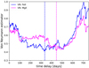 |
Fig. B.1. Von Neumann estimator for the total Mg II (magenta) and the total Fe II (blue) emission after the removal of four data points (9, 17, 18, 26). The vertical dashed lines denote the corresponding minima. |
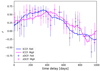 |
Fig. B.2. Correlation function for the total Mg II (magenta) and the total Fe II (blue) emission after the removal of four points (9, 17, 18, 26). The solid lines denote the ICCF, while the points with error bars stand for the zDCF method. |
All Tables
Overview of the time-delay determinations for the total Mg II and Fe II total line emissions.
Time-delay measurements for seven wavelength bins containing a combination of Mg II and Fe II emission, after subtracting the power-law component.
Summary of the time-delay peak and centroid values for different methods (expressed in days in the observer’s frame) with the four observations (9, 17, 18, and 26) that were omitted in the Mg II and Fe II light curves.
Instruments are 1 – OGLE, 2 – SALT, 3 – BMT, 4 – SSO, 5 – lesedi, 6 – CTIO, 7 – SAAO.
All Figures
|
Fig. 1. Observation 36 from the SALT telescope (red) and the model (black). The dashed green line shows the underlying continuum from the accretion disk, the dotted blue line is the Fe II pseudo-continuum, and the dotted magenta lines represent the two kinematic components of the Mg II line. |
| In the text | |
|
Fig. 2. Long-term photometric light curve (upper panel), including CATALINA measurements (light green shaded region) from Czerny et al. (2019), and total Mg II (middle panel) and Fe II (lower panel) light curves. Photometric observations are in magnitudes (panel 1), but Mg II and Fe II fluxes are in units of 10−16 and 10−17 erg s−1 cm−2. We used only the non-shaded region. |
| In the text | |
|
Fig. 3. Interpolated cross-correlation function as a function of the time delay in the observer’s frame for the total Mg II (magenta line) and the total Fe II emission (blue line). The dashed vertical lines mark the corresponding time-delay peak values. The correlation coefficient at the peak value for the Fe II pseudo-continuum is larger than the correlation coefficient at the time-delay peak of the Mg II line. The dotted horizontal line marks r = 0.5. We also show the previous ICCF (Czerny et al. 2019) when the peak time delay was at ∼1064 days; see the solid gray line. Cont:79 and line:26 represents the number of observations used in (Czerny et al. 2019). |
| In the text | |
|
Fig. 4. χ2 value as a function of the time delay in the observer’s frame for the Mg II line emission (magenta line) as well as for the Fe II line emission (blue line). The global χ2 minima for each line are depicted by the vertical dashed lines. The χ2 time-delay dependence for the previous, shorter continuum-Mg II light curves (Czerny et al. 2019) is shown as a gray line with the global minimum at the time delay twice as large as for the current data. Cont:79, 113 and line:26, 35 represents the number of observations. |
| In the text | |
|
Fig. 5. Von Neumann estimator as a function of the time delay in the observer’s frame for the total Mg II (magenta line) and Fe II (blue line) emissions. The dashed vertical line marks the common global minimum of the von Neumann estimator at ∼512.0 days. |
| In the text | |
|
Fig. 6. Bartels estimator as a function of the time delay in the observer’s frame for the total Mg II (magenta line) and Fe II (blue line) emissions. The dashed vertical line marks the common global minimum of the Bartels estimator at ∼512.0 days. |
| In the text | |
|
Fig. 7. zDCF correlation coefficient as a function of the time delay in the observer’s frame for the total Fe II (blue line) and the total Mg II emission (magenta line). The vertical lines denote the peak values for each corresponding line. |
| In the text | |
|
Fig. 8. First column: continuum light curve in magnitude (first panel) and the seven curves in different wavebands derived from the combination of photometric and the spectroscopic observations (remaining panels). The corresponding waveband ranges are listed in Table 3. Curves 1 and 7 are in unit of 10−17 and other curves are in 10−16. Second column: auto-correlation of continuum and the ICCF results for all the curves with respect to continuum. Histograms are the peak (red) and centroid (blue) distribution from the ICCF with 10 000 bootstrap realizations. |
| In the text | |
|
Fig. 9. ICCF and χ2 values as a function of time delay. Left panel: ICCF as a function of time delay (expressed in days in the observer’s frame) for the seven light curves according to the legend. Right panel: χ2 value as a function of the time delay (in days) in the observer’s frame for the seven light curves according to the legend. |
| In the text | |
|
Fig. 10. Wavelength-dependent time lags from various methods along with the mean and RMS spectrum. Time lags seem to weakly follow the RMS spectrum. |
| In the text | |
|
Fig. 11. Estimators of data randomness/regularity as a function of the time delay in the observer’s frame. Left panel: von Neumann estimator for seven Mg II line light curves according to the legend. Right panel: Bartels estimator value for the same Mg II light curves in the observer’s frame. The dashed red line represents the estimated time delay. |
| In the text | |
|
Fig. 12. z-transformed DCF as a function of the time delay in the observer’s frame for individual light curves according to the legend. Overall, there is a time-delay peak between 300 and 400 days, consistent within the uncertainties for all the light curves. We highlight the shift of ∼40 days between the time-delay peaks of the first and fifth waveband by using the corresponding horizontal lines to denote the peak values. |
| In the text | |
|
Fig. 13. Javelin bootstrap results with 1000 realizations for all the seven curves (from left to right). The peak and results from this are listed in Table 4. |
| In the text | |
|
Fig. 14. Auto-correlation function of total Mg II and total Fe II along with the continuum. |
| In the text | |
|
Fig. 15. Schematic representation of the Mg II and Fe II emission regions. The mean distance of the Mg II and Fe II region from the BH is ∼0.23 pc, estimated from the rest frame time delays, 276 days and 270 days for Mg II and Fe II, respectively. The Fe II emission also exhibits a shorter time delay in the rest frame, 180 days, which indicates the larger extent of the Fe II region with respect to the Mg II emission region in the direction away from the SMBH. Hence, due to a non-negligible inclination of the observer, the reprocessed emission from the Fe II region finally tends to come to the observer sooner. The secondary time delays at ∼570 and ∼680 days can potentially be attributed to the mirror-effect, i.e., the Mg II and Fe II emission, respectively, coming to the observer from the other side of the accretion disc, which is supported by the temporal difference of (570 − 270) = 300 days, which corresponds to ∼0.25 pc, i.e., one additional disk crossing of photons. However, the Fe II emission coming from the more distant part across the disk is partially shielded by the Mg II line-emitting region closer in with respect to the observer. Color does not represent the density of the cloud. |
| In the text | |
|
Fig. 16. Radius-luminosity relation for the currently available 78 Mg II sources. The best-fit relation determined by the classical least-squares fitting is indicated by the solid green line. The updated Mg II emission-line time delay of |
| In the text | |
|
Fig. 17. Mg II maximum likelihood RL relation determined using the MCMC algorithm (left panel). The coefficients as well as the RMS scatter are consistent within the uncertainties with the classical fitting algorithm (see Fig. 16). CTS C30.10 is depicted using the black circle, while the previous time-delay measurement, approximately twice as long, is represented by a gray circle. The dashed violet line shows the Bentz RL relation with a slope of ∼0.5, which was adjusted for the continuum luminosity at 3000 Å. Right panel: corner plot representation of the distribution histograms for the two parameters α (slope) and K constant in the linear fit of logτ = α log L44 + K to the Mg II data. The likelihood function is included the underestimation factor f, whose distribution is also shown. |
| In the text | |
|
Fig. 18. Extended RL relation including the relative Fe II strength, RFe II. Left panel: median relation (blue line) is inferred by maximizing the likelihood function. Green lines show 1000 random selections from the parameter distribution. 66 Mg II time-delay measurements are color-coded to depict log RFe III according to the color axis on the right. The RMS scatter is 0.28 dex. Right panel: corner plot shows the parameter distributions inferred from the MCMC method. The parameter uncertainties correspond to 16th and 84th percentiles. |
| In the text | |
|
Fig. 19. Preliminary RL relation for the UV Fe II pseudo-continuum based on the two time-lag measurements for NGC 5548 (Maoz et al. 1993) and CTS C30.10 (this work). We derive two relations based on the two Fe II time delays for CTS C30.10: 180.3 days and 270.0 days. The longer time delay of 270.0 days is more consistent with the RL relation derived by Bentz et al. (2013) when renormalized to the 3000 Å monochromatic luminosity. The shaded regions depict 1σ confidence intervals of individual RL relations. |
| In the text | |
|
Fig. B.1. Von Neumann estimator for the total Mg II (magenta) and the total Fe II (blue) emission after the removal of four data points (9, 17, 18, 26). The vertical dashed lines denote the corresponding minima. |
| In the text | |
|
Fig. B.2. Correlation function for the total Mg II (magenta) and the total Fe II (blue) emission after the removal of four points (9, 17, 18, 26). The solid lines denote the ICCF, while the points with error bars stand for the zDCF method. |
| In the text | |
Current usage metrics show cumulative count of Article Views (full-text article views including HTML views, PDF and ePub downloads, according to the available data) and Abstracts Views on Vision4Press platform.
Data correspond to usage on the plateform after 2015. The current usage metrics is available 48-96 hours after online publication and is updated daily on week days.
Initial download of the metrics may take a while.