| Issue |
A&A
Volume 666, October 2022
|
|
|---|---|---|
| Article Number | A84 | |
| Number of page(s) | 20 | |
| Section | Extragalactic astronomy | |
| DOI | https://doi.org/10.1051/0004-6361/202244030 | |
| Published online | 10 October 2022 | |
The miniJPAS survey
The role of group environment in quenching star formation
1
Instituto de Astrofísica de Andalucía (CSIC), PO Box 3004, 18080 Granada, Spain
e-mail: This email address is being protected from spambots. You need JavaScript enabled to view it.
2
Departamento de Física, Universidade Federal de Santa Catarina, PO Box 476, 88040-900 Florianópolis, SC, Brazil
3
Zentrum für Astronomie, Universität Heidelberg, Philosophenweg 12, 69120 Heidelberg, Germany
4
Institut für Theoretische Physik, Universität Heidelberg, Philosophenweg 16, 69120 Heidelberg, Germany
5
Observatório do Valongo, Universidade Federal do Rio de Janeiro, 20080-090 Rio de Janeiro, RJ, Brazil
6
Department of Physics, University of Helsinki, Gustaf Hällströmin katu 2, 00014 Helsinki, Finland
7
Gemini Observatory/NSF’s NOIRLab, Casilla 603, La Serena, Chile
8
Centro de Estudios de Física del Cosmos de Aragón (CEFCA), Plaza San Juan 1, 44001 Teruel, Spain
9
Instituto de Física, Universidade de São Paulo, Rua do Matão 1371, 05508-090 São Paulo, Brazil
10
Departamento de Astronomia, Instituto de Física, Universidade Federal do Rio Grande do Sul (UFRGS), Av. Bento Gonçalves 9500, Porto Alegre, R.S, Brazil
11
Observatório Nacional, Ministério da Ciencia, Tecnologia, Inovação e Comunicações, Rua General José Cristino, 77, São Cristóvão, 20921-400 Rio de Janeiro, Brazil
12
Department of Astronomy, University of Michigan, 311 West Hall, 1085 South University Ave., Ann Arbor, USA
13
Department of Physics and Astronomy, University of Alabama, Box 870324 Tuscaloosa, AL, USA
14
Donostia International Physics Center (DIPC), Manuel Lardizabal Ibilbidea 4, San Sebastián, Spain
15
Ikerbasque, Basque Foundation for Science, 48013 Bilbao, Spain
16
Instituto de Física, Universidade Federal da Bahia, 40210-340 Salvador, BA, Brazil
17
Instituto de Física de Cantabria (CSIC-UC), Avda. Los Castros s/n., 39005 Santander, Spain
18
Universidade de São Paulo, Instituto de Astronomia, Geofísica e Ciências Atmosféricas, R. do Matão 1226, 05508-090 São Paulo, Brazil
19
Centro de Estudios de Física del Cosmos de Aragón (CEFCA), Unidad Asociada al CSIC, Plaza San Juan 1, 44001 Teruel, Spain
Received:
16
May
2022
Accepted:
11
July
2022
Abstract
The miniJPAS survey has observed ∼1 deg2 of the AEGIS field with 60 bands (spectral resolution of R ∼ 60) in order to demonstrate the scientific potential of the Javalambre-Physics of the Accelerating Universe Astrophysical Survey (J-PAS), which will map ∼8000 deg2 of the northern sky over the coming years. In particular, this paper demonstrates the potential of J-PAS in detecting groups with mass of up to 1013 M⊙ and in characterising their galaxy populations up to z ∼ 1. The parametric code BaySeAGal is used to derive the stellar population properties by fitting the J-PAS spectral energy distribution (SED) of the galaxy members in 80 groups at z ≤ 0.8 previously detected by the AMICO code, and of a galaxy field sample retrieved from the whole miniJPAS down to r < 22.75 (AB). Blue, red, quiescent, and transition (blue quiescent or green valley) galaxy populations are identified through their rest-frame (extinction-corrected) (u − r)int colour, galaxy stellar mass (M⋆), and specific star formation rate (sSFR). We measure the abundance of these galaxies as a function of M⋆ and environment in order to investigate the role that groups play in quenching star formation. Our findings are as follows. (i) The fraction of red and quiescent galaxies in groups increases with M⋆ and is always higher in groups (28% on average) than in the field (5%). (ii) The quenched fraction excess (QFE) in groups shows a strong dependence on M⋆, and increases from a few percent for galaxies with M⋆ < 1010 M⊙ to higher than 60% for galaxies with M⋆ > 3 × 10¹¹ M⊙. (iii) The abundance excess of transition galaxies in groups shows a modest dependence on M⋆, being 5%–10% for galaxies with M⋆ < 1011 M⊙. (iv) The fading timescale, defined as the time that galaxies in groups spend in the transition phase, is very short (< 1.5 Gyr), indicating that the star formation of galaxies in groups declines very rapidly. (v) The evolution of the galaxy quenching rate in groups shows a modest but significant evolution since z ∼ 0.8. This latter result is compatible with the expected evolution with constant QFE = 0.4, which has been previously measured for satellites in the nearby Universe, as traced by SDSS. Further, this evolution is consistent with a scenario where the low-mass star forming galaxies in clusters at z = 1–1.4 are environmentally quenched, as previously reported by other surveys.
Key words: galaxies: evolution / galaxies: stellar content / galaxies: groups: general / galaxies: photometry / galaxies: fundamental parameters
© R. M. González Delgado et al. 2022
 Open Access article, published by EDP Sciences, under the terms of the Creative Commons Attribution License (https://creativecommons.org/licenses/by/4.0), which permits unrestricted use, distribution, and reproduction in any medium, provided the original work is properly cited.
This article is published in open access under the Subscribe-to-Open model. This email address is being protected from spambots. You need JavaScript enabled to view it. to support open access publication.
1. Introduction
Today, the bimodal distribution of galaxy populations is well known. The Sloan digital sky survey (SDSS) has provided abundant evidence that galaxies in the nearby Universe (z < 0.1) inhabit two specific loci of the colour–magnitude diagram (CMD), the red sequence and the blue cloud (Blanton & Moustakas 2009). Nearby galaxies in the red sequence are generally characterised by a red, old, and metal-rich stellar population; whereas galaxies in the blue cloud are mainly star forming galaxies with blue colours, and with young, less-metal-rich stars dominating the optical light (Kauffmann et al. 2003a,b; Baldry et al. 2004; Brinchmann et al. 2004; Gallazzi et al. 2005; Mateus et al. 2006; Asari et al. 2007; González Delgado et al. 2014). This bimodal distribution of the galaxy populations persists at higher redshift (Bell et al. 2004; Williams et al. 2009; Whitaker et al. 2010; Hernán-Caballero et al. 2013; Díaz-García et al. 2019a,b,c; González Delgado et al. 2021). However, since z ∼ 1, a large fraction of the blue galaxies has seen its star formation truncated and has evolved towards the red and quiescent galaxy population, although this is mostly seen for galaxies with stellar mass lower than 1010 M⊙ (Díaz-García et al. 2019b). The transition from blue to red galaxies must occur in a short period of time because the number density of the red galaxies has roughly doubled since z ∼ 1 and the number density of the ‘green valley’ galaxies, which lie in between the red sequence and blue cloud objects in the CMD, is not enough to explain the evolution in number (Bell et al. 2004; Faber et al. 2007; Muzzin et al. 2013). This process of transformation from the blue cloud to the red sequence is called quenching.
There is a correlation between the colour and the mass of galaxies belonging to each population. In the local Universe, the galaxies in the red sequence are more massive than galaxies in the blue cloud (Kauffmann et al. 2003a,b; Baldry et al. 2004; Cid Fernandes et al. 2005; González Delgado et al. 2014). However, at intermediate redshifts (z ∼ 1) this relation is more complex (see e.g., Ilbert et al. 2013). The stellar mass (M⋆) is a relevant galaxy property that correlates with other indicators of galaxy evolution (Pérez-González et al. 2008; Pérez et al. 2013; Schawinski et al. 2014; López Fernández et al. 2018). In particular, M⋆ is related to the quenching process known as mass-quenching (Peng et al. 2010; Kovač et al. 2010). This is based on the strong correlation between the fraction of red galaxies and the stellar mass (Kauffmann et al. 2003a; Baldry et al. 2006), and the assumption of red colours as a proxy for a quenched stellar population. Further, galaxies that have shut down their star formation are also referred to as quenched. They are no longer in the relation between star formation rate and stellar mass known as the star forming main sequence (Noeske et al. 2007; Speagle et al. 2014; Renzini & Peng 2015; González Delgado et al. 2016; López Fernández et al. 2018; Thorne et al. 2021), and have reduced their specific star formation rate (sSFR) by a factor of 10–100. Mass quenching is an internal process that is not necessarily caused by the galaxy stellar mass. Other properties, such as the halo mass (e.g., Behroozi et al. 2019) or the black-hole mass (e.g., Bluck et al. 2019, 2020), both of which correlate with M⋆, may be related to mass quenching.
Besides the stellar mass, the evolution of the galaxy population is also a function of the environment (Balogh et al. 2004; Blanton et al. 2005). Unlike mass quenching, environmental quenching is associated with external processes acting in dense environments such as galaxy groups and clusters. Processes such as ram-pressure stripping (Abadi et al. 1999), galaxy harassment (Moore et al. 1996), starvation (Larson et al. 1980), galaxy-cluster tidal interaction (Merritt 1984; Bekki 1999), viscous stripping (Nulsen 1982), and thermal evaporation (Cowie & Songaila 1977) can eventually shut down or suppress star formation by heating and/or removing the gas from the galaxies. Since the pioneering work of Dressler (1980), many studies have demonstrated the dependence of the distribution of galaxy populations and of their properties on environmental density (e.g., Kauffmann et al. 2004; Blanton & Moustakas 2009; Pasquali et al. 2010; Lopes et al. 2014; Cappellari 2016). There is strong evidence that the fraction of red galaxies increases with the density field for z < 1 (Woo et al. 2013; Nantais et al. 2016; Darvish et al. 2016; Calvi et al. 2018; Moutard et al. 2018; Liu et al. 2021; McNab et al. 2021; Sobral et al. 2022), although the quenched fraction is less significant at higher redshift. This result is equivalent to the well-known Butcher-Oemler effect (Butcher & Oemler 1984), which shows that the fraction of blue galaxies in clusters increases with redshift.
Mass and environmental quenching can both be explained by the halo quenching process, which is due to the connection between stellar mass, environment, and the halo mass. The gas in massive galaxy-scale halos (> 1012 M⊙) is prevented from efficiently cooling as it becomes shock-heated (Dekel & Birnboim 2006), and the cessation of gas accretion along with ram-pressure stripping prevents further star formation in galaxies, leading to the evolution of galaxies at z ∼ 1 from blue to red. Moreover, mass and environmental quenching are independent processes because the most massive galaxies are quenched independently of their environment, and galaxies in dense environments are quenched independently of their stellar mass (Peng et al. 2010). Furthermore, Peng et al. (2012) and Kovač et al. (2014) found little evidence of a dependence of the red fraction of central galaxies on overdensity, whereas satellite galaxies are the main ‘victims’ of environmental quenching in the galaxy population. Satellite galaxies are consistently redder at all overdensities, and quenching efficiency increases with overdensity at 0.1 < z < 0.4 (Kovač et al. 2014). It has been suggested that satellite quenching also depends on the distance to the centre of the halo, and for satellites at lower distance to the halo, quenching depends strongly on the mass halo rather than on stellar mass (Woo et al. 2013).
Galaxy surveys have been very successful in detecting high-density structures, which can be used to study the quenching processes as a function of global environment (clusters, groups, filaments, voids) or of local density, through different definitions of the galaxies number density. Good examples are SDSS (e.g., Yang et al. 2007) and MaNGA (Bluck et al. 2020) at low redshifts; and zCOSMOS (Peng et al. 2012), CANDELS (Liu et al. 2021), GOGREEN (Balogh et al. 2017; McNab et al. 2021), CLASH-VLT (Rosati et al. 2014; Mercurio et al. 2021), and LEGA-C (Sobral et al. 2022) at higher redshifts. In general, multi-wavelength photometry and spectroscopic information are combined to get accurate redshifts and to identify the group and cluster galaxy members. Galaxy colours, emission line properties, galaxy mass, and star formation rates (SFR) are then derived as proxies to identify the quenched galaxy populations. However, other surveys such as the Hyper Suprime-Cam Subaru Strategic Program (HSC-SSP) combine only deep broad-band photometry with a few narrow band filters to identify group and cluster galaxy members (Lin et al. 2017; Jian et al. 2018; Nishizawa et al. 2018) and emission line galaxies (ELG, Koyama et al. 2018; Hayashi et al. 2018). In this case, Hα or [OIII] nebular lines at a given redshift are detected, without distinguishing between recent star formation in the galaxy and active galactic nucleus (AGN) contribution.
The Javalambre-Physics of the Accelerating Universe Astrophysical Survey (J-PAS, Benítez et al. 2009, 2014) was conceived in order to overcome the limitations of combining broad-band multiwavelength and spectroscopic surveys. J-PAS is a multi-wavelength imaging survey of ∼8000 deg2 in the northern sky that is being carrying out with the 2.5 m telescope at the Javalambre Astrophysical Observatory (OAJ; Teruel, Spain) (Cenarro et al. 2014).
The photometric system, composed of multi-wavelength narrow bands, is equivalent to a low-resolution spectroscopy of R ∼ 60. It was designed to measure photo-z with an accuracy of up to Δz = 0.003 (1 + z) (Benítez et al. 2014; Bonoli et al. 2021; Hernán-Caballero et al. 2021). The large area of the survey, the characteristics of the imaging camera, and the accuracy of the photo-z allow us to perform multiple cosmological and galaxy evolution studies. This combination enables us to derive the number density of galaxy clusters as a function of redshift and mass to constrain cosmological parameters. With this setup, we are able to map clusters and groups up to z ∼ 1 and with relatively small masses, producing a complete and mass-sensitive cluster and group catalogue, in order to study the role of environment in galaxy evolution.
As a low-resolution spectroscopic survey, J-PAS allows us to identify the emission line galaxy population in a continuum range of redshifts up to z ∼ 1.4 through [OII], Hβ, [OIII], Hα, and [NII] nebular lines. The emission line diagnostics, such as [NII]/Hα and [OIII]/Hβ, allow us to discern between AGN and star forming galaxies up to z ∼ 0.35 (Martínez-Solaeche et al. 2021). Furthermore, we have already proven the power of J-PAS to identify and characterise the emission-line galaxy population in the AEGIS field (Martínez-Solaeche et al. 2022) making use of the miniJPAS survey. Briefly, miniJPAS is a proof-of-concept small survey covering ∼1 deg2, taken with the same photometric system as J-PAS and the Pathfinder camera (Bonoli et al. 2021). The photo-z is derived for 17 500 galaxies per deg2 with rSDSS < 23, of which ∼4200 have |Δz|< 0.003 (Hernán-Caballero et al. 2021). Moreover, with miniJPAS we have shown the capability of the J-PAS filter system to dissect the bimodal distribution of red and quenched and blue and star-forming galaxy populations and their evolution up to z ∼ 1 (González Delgado et al. 2021).
In this work, we discuss the role of group environment in quenching galaxies by comparing the properties of the group members detected in the extended growth strip with the galaxies that are in lower density environments, that is, in the field. For this, we use the miniJPAS survey and the group catalogue constructed using the Adaptive Matched Identifier of Cluster Objects (AMICO) code (Maturi et al. 2005). Our purpose is to show the power of J-PAS to search for the role that environment plays in the evolution of galaxies; in particular to quench their star formation. The accuracy of the photo-z (Hernán-Caballero et al. 2021) provided by miniJPAS allowed us to retrieve a group catalogue with halo masses down to several times 1013 M⊙ (Maturi et al. in prep). Further, the analysis of the multi-band data of miniJPAS (J-spectra, hereafter) with the full spectra fitting method adapted to multi-narrowband (NB) data allows us to obtain the star formation histories of the galaxies, which in turn allow us to identify the quenched galaxy population in groups and in lower density environments.
This paper is structured as follows. Section 2 briefly describes the data and properties of the sample analysed here. Section 3 explains the method used to fit the J-spectra, the classification of galaxies according to their environment, and the identification of the most massive galaxy in each group. In Sect. 4 we present the inferred stellar population properties of the galaxies, and we compare the properties of galaxies in groups and in the field. Section 5 presents the fraction of red and blue galaxies as a function of local density and global environment. In Sect. 6 we discuss the results in terms of the excess of the quenched fractions in groups, and the evolution of the galaxy quenched rate in groups. Finally, the results are summarised in Sect. 7.
Throughout the paper we assume a Lambda cold dark matter (ΛCDM) cosmology in a flat Universe with H0 = 67.4 km s−1 and ΩM = 0.315 (Planck Collaboration VI 2020). All the stellar masses in this work are quoted in solar mass units (M⊙) and are scaled according to a universal (Chabrier 2003) initial stellar mass function. All the magnitudes are in the AB-system (Oke & Gunn 1983).
2. The data and sample
2.1. Data: observations and calibration
The observations consist of four pointings in the extended growth strip covering an area of ∼1 deg2. The data are from the miniJPAS survey (Bonoli et al. 2021) and were obtained with the 2.5 m Javalambre Survey Telescope (JST/T250) located at the OAJ (Cenarro et al. 2019) with the Pathfinder camera. The miniJPAS data were obtained with the J-PAS photometric system that contains 54 narrow-band filters of full width at the half maximum (FWHM) of 145 Å equally spaced every ∼100 Å covering 3780 to 9100 Å, plus two mid-band filters centred at 3479 Å and 9316 Å, and the broad SDSS bands u, g, r, i. This system is equivalent to a spectral resolution of R ∼ 60.
The observations were processed by the Data Processing and Archiving Unit group at Centro de Estudios de Física del Cosmos de Aragón (CEFCA; Cristóbal-Hornillos et al. 2014) as described in Bonoli et al. (2021). The photo-z were estimated by the JPHOTOZ package developed at CEFCA using a customised version of the LEPHARE code (Arnouts et al. 1999). A new set of stellar population synthesis galaxy templates was optimised for the miniJPAS filter system (Hernán-Caballero et al. 2021). The results show that miniJPAS at rSDSS < 23, has ∼17 500 galaxies with valid JPHOTOZ estimates, ∼4200 of which are expected to have |Δz|< 0.003. All the images and associated catalogues are publicly available at1.
2.2. Sample
The galaxy sample used in this work is an extension of that analysed in González Delgado et al. (2021). It was retrieved from the dual-mode miniJPAS catalogue, selecting according to rSDSS ≤ 22.75 (MAG_AUTO), and redshift (photo − z ≤ 1). We also use the ‘stellar-galaxy locus classification’ total_prob_star parameter (López-Sanjuan et al. 2019; Baqui et al. 2021) listed in the miniJPAS photometry catalogue to select extended sources (total_prob_star ≤ 0.5). We use as photo-z the lephare_z_ml parameter listed in the miniJPAS catalogue provided by (Hernán-Caballero et al. 2021), which is the median redshift of the probability density function (PDF) of the photo-z distribution for each object. In total, we select 11281 objects; and we were able to get a reasonable SED fit for 99% of the galaxies in the sample (see Sect. 3). These selection criteria are very similar to those used by Maturi et al. (in prep.) to identify galaxy groups and clusters in miniJPAS.
3. Analysis
3.1. The J-spectra fits
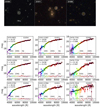 |
Fig. 1. Images and J-spectra of several galaxy members in three AMICO groups. Upper panel: images of the central part of G1054, G1011, and G1005. The most massive galaxy in each group is marked with a circle. Middle and bottom panels: J-spectra (MAG_AUTO) of galaxy members of G1054, G1011, and G1005, as labelled. The most massive galaxy (marked with a circle in the upper panel), the second most massive galaxy in each group, and other galaxy members of the group are shown. J-spectra are shown as coloured dots, while the best model fitted by BaySeAGal for each J-spectrum is plotted as a black point; the grey band shows the magnitudes of the mean model ± one σ uncertainty level. The differences between the observed and best model fitted magnitudes are plotted as small coloured points around the black bottom line. Masked filter (white circles) and filters overlapping with the emission lines Hα, [NII], [OIII], Hβ, and [OII] (grey circles) are not used in the fits. The dashed vertical lines show the wavelength positions where the Hα, [OIII], and [OII] could be in emission at the redshift of each galaxy. The Hα line is clearly detected in the galaxies 2243-12307 and 2243-12394 that belong to G1011, and 2470-10291 of G1054. |
To estimate the stellar population properties of the galaxies as a function of the environmental conditions, we fit the J-spectra with a SED-fitting code. Figure 1 shows several examples of the J-spectra of galaxies that belong to three AMICO groups, at redshift ∼0.07, 0.27, and 0.57. Red galaxies and galaxies with Hα emission (presumably star-forming galaxies) are present in these groups. The signal-to-noise ratio (S/N) and the quality of the J-spectra are very similar for the red and blue galaxy populations in miniJPAS (González Delgado et al. 2021).
Here, we use the SED-fitting code BaySeAGal (González Delgado et al. 2021) to fit the J-spectra. This is a Bayesian parametric code that assumes the latest versions of the Bruzual & Charlot (2003) stellar population synthesis models (Plat et al. 2019, hereafter C&B). The C&B models follow the PARSEC evolutionary tracks (Marigo et al. 2013; Chen et al. 2015) and use the Miles (Sánchez-Blázquez et al. 2006; Falcón-Barroso et al. 2011; Prugniel et al. 2011) and IndoUS (Valdes et al. 2004; Sharma et al. 2016) stellar libraries in the spectral range covered by the J-spectra data.
The code assumes a SFH2 =SFH(t; Θ), where t is the lookback time and Θ is a parameter vector that includes the stellar metallicity (Z⋆), a dust attenuation parameter (AV), and the parameters (k, t0, τ) that control the time evolution of the SFR3, ψ(t). We assume a delayed-τ model of the form:
![Mathematical equation: $$ \begin{aligned} \psi (t) = k \frac{t_0-t}{\tau }\exp { \left[ -(t_0-t)/\tau \right] }, \end{aligned} $$](/articles/aa/full_html/2022/10/aa44030-22/aa44030-22-eq1.gif) (1)
(1)
where t0 is the time of the onset of the star formation in lookback time, τ is the SFR e-folding time, and k is a normalisation constant related to the total mass formed in stars. The galaxy stellar mass is calculated from the mass converted into stars according to the SFH and the luminosity of the galaxy, and taking into account the mass loss of the single stellar population synthetic models owing to stellar evolution.
BaySeAGal follows a Markov chain Monte Carlo (MCMC) approach that explores the parameter space and constrains the parameters of the SFH that fit the J-spectra. The code allows us to retrieve the chains and their χ2 likelihood, to derive the PDF for each of the stellar population properties (stellar mass, stellar age, dust attenuation, stellar metallicity, and colours), and the median and sigma of the chains as its inferred value and error.
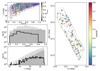 |
Fig. 2. Observational properties of the sample and distribution of the AMICO galaxy members. Upper-left panel: redshift–magnitude diagram for the whole sample colour coded according to the probabilistic association, Passoc. Middle-left panel: redshift distribution. Bottom panel: rSDSS (MAG_AUTO) distribution. Here we show the galaxies in a group environment (black line), and galaxies in the field (grey histograms). The distributions of the full miniJPAS sample of galaxies are also shown (light grey histograms). Right panel: contours show the density galaxy map distribution of the whole miniJPAS sample analysed here. The points show the distribution of galaxies in groups; the circles are the brightest and most massive galaxy of each AMICO group. Points are coloured according to photo-z. |
The solutions from the J-spectra fits reproduce the 56 miniJPAS magnitudes of galaxies of different types quite well within the uncertainties and independently of the redshift and brightness range (e.g., Fig. 1). The emission lines from young star forming regions and/or AGN contributions are not fitted with this code. Therefore, the NBs affected by the contribution of the most relevant lines, Hα, Hβ, [NII]λ6584, 6548, [OIII]λ5007, 4959, and [OII]λ3727, are removed from the J-spectra fit at the redshift of each galaxy, which means that the fits are restricted to the stellar continuum.
A more detailed explanation of the inputs and assumptions in the code and how the results compare with other codes such as MUFFIT (Díaz-García et al. 2015), AlStar (Batista et al. in prep.), and TGASPEX (Magris et al. 2015) can be found in González Delgado et al. (2021).
3.2. Galaxy classification versus environment
The Adaptive Matched Identifier of Cluster Object (AMICO) code (Maturi et al. 2005; Bellagamba et al. 2018) is used in miniJPAS for the detection of galaxy groups and clusters. The code is based on an optimal filtering approach, which minimises the noise variance under the condition that the estimated signal is unbiased. Using the redshift of the galaxies, their magnitudes, sky position, and the background noise as input, the code provides a factor called amplitude and the association probability (Passoc) for each galaxy, this latter being the probability that the galaxy is a member of a cluster or group. Because the different clusters can overlap in the data space, more than one cluster association can be assigned to the same galaxy through an iterative approach, with the new  , where the sum is extended to the probabilities of the previous cluster and group assignments. This is a key parameter in our study because it allows us to identify the galaxy members of a group or cluster, and therefore to characterise the galaxy populations in terms of global environment.
The good performance of AMICO and miniJPAS regarding mass sensitivity, mass-proxy quality, and redshift accuracy show that J-PAS will allow us to derive cosmological constraints not only based on cluster counts but also on clustering of galaxy clusters (Maturi et al. in prep.). From this analysis, AMICO identified ∼80 groups in miniJPAS at z < 1 down to 1013 M⊙, when the photo-z defined as the lephare_z_ml is taken as the galaxy redshift, and the rSDSS (MAG_AUTO) as inputs to the code.
To identify and characterise the galaxy populations in terms of group environment, we assign a Passoc to each galaxy of the sample. For this purpose, we perform a cross match of the catalogues with the galaxy group members and the miniJPAS galaxies. As mentioned above, a galaxy can have a Passoc of greater than zero in more than one of the galaxy groups in the catalogue, and so in our analysis we only consider the highest Passoc among those for this galaxy. If a galaxy is not listed in any of the group catalogues, we set the Passoc of this galaxy equal to zero.
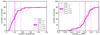 |
Fig. 3. Left panel: cumulative distribution of the number of galaxy members in the AMICO groups. The distribution is derived for three values of Passoc as indicated in the inset. The vertical solid line is the average number of galaxy members per group; the dashed lines show ±1 sigma. Right panel: cumulative distribution of the group stellar mass. |
Roughly half of the galaxies of the sample (49%) are not listed in any of the group catalogues, indicating that they are not within a group environment; in contrast, only 14% of the miniJPAS galaxies have Passoc ≥ 0.5, and 7% have Passoc ≥ 0.7. We use Passoc to segregate the galaxy populations into two different environments: galaxies in groups if Passoc ≥ 0.7, and galaxies in the field if Passoc ≤ 0.1. These two subsamples are very different in number, 7% and 63% of the galaxies belong to group and field environments, respectively. However, they show similar range in magnitude (Fig. 2). In terms of redshift, a few galaxies in groups are detected at z > 0.8. As expected, the galaxies in groups trace the most dense areas of miniJPAS galaxy populations (right panel in Fig. 2). In addition to these two subsamples, we consider the galaxies with 0.1 < Passoc< 0.7 as part of the whole AEGIS sample.
3.3. Group stellar mass
Most of the high-density structures detected by AMICO contain a number of galaxies that is typical of galaxies groups. As Fig. 3 shows, half of the structures have less than ten galaxies per group (typical value = 10.4 ± 7.4), which is a number more typical of groups than clusters. However, this number shows a strong dependence on Passoc (Fig. 3). It varies from ∼5 (Passoc ≥ 0.8) to ∼15 (Passoc ≥ 0.6) galaxy members. However, even the highest values are still below the typical value of galaxy members in clusters. One exception is G1001, named mJPC2470-1771 (Rodríguez Martín et al. 2022). This is the only one that has > 50 galaxy members, and it can be considered a cluster (the most massive miniJPAS cluster).
The halo masses obtained through the scaling relation have values in the range of galaxy groups (in the order of 1013 M⊙) (Maturi et al., in prep.). It is also known that the mass of the dark matter halo associated with a group is well correlated with the total stellar mass of the group, and with the mass of the most massive galaxy in the group (Yang et al. 2007). Here, we can estimate the stellar mass of each group by adding the individual galaxy stellar mass. It is worth noting that the stellar mass of a galaxy is expected to be approximately 1%–2% of its ‘halo’ mass (Moster et al. 2010; Behroozi et al. 2013). Figure 3 shows the distribution of the group stellar mass of the AMICO groups. Half of the AMICO groups have log  [M⊙]. Only, mJPC2470-1771 has log
  [M⊙], and a halo mass from the scaling relation which is above 1014 M⊙. In contrast to the number of galaxies in each group,
  shows a weak dependence on Passoc for 0.6 ≤ Passoc ≤ 0.8 (Fig. 3). We can therefore conclude that, given the number of members and the stellar mass, these AMICO structures are groups. However,
  is ∼0.11 dex lower than the total group mass calculated by weighting each galaxy M⋆ by its Passoc and adding all the galaxies with Passoc > 0.5.
3.4. Identification of the most massive and brightest central galaxy in each group
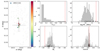 |
Fig. 4. Distribution in the sky of the galaxy members listed in the catalogue of the AMICO group G52 (left panel). Objects in the catalogue with Passoc < 0.7 are plotted with grey dots. The galaxies with Passoc (≥0.7) are shown with circles that are coloured according to their Passoc. The most massive galaxy and the galaxy with the highest Passoc are marked by a red and a cyan cross, respectively. The group centre is also marked with a large black cross. Right panels: distribution of Passoc in the catalogue, the stellar mass, absolute magnitude in the r band, and redshift. The position of the BGG is marked with a red vertical line. The distribution of the galaxy members (Passoc ≥ 0.7) is shown with the black histogram. |
The brightest cluster galaxy (BCG) is the brightest galaxy within the high-density structure, which is located at the geometrical and kinematic centre of the cluster if it is in equilibrium. Usually, it is a massive and red early-type galaxy at the centre of the potential well, which in many cases is coincident with the maximum of the X-ray emission. However, the structures found in miniJPAS by AMICO are not particularly big; they are mainly groups, as we have already pointed out. The identification of the brightest and most central galaxy of each group is not easy, because the brightest and the most massive galaxy do not have to be at the centre of the structure.
First, we need to determine the geometrical centre of the group. For this we only use the first five galaxies with the highest Passoc that are listed in the AMICO catalogue of each group. A distance probability (Pdist) is then associated to each galaxy group member; this scales with the distance in a linear way and is equal to one for the galaxy that is closest to the centre, and zero for the galaxy that is at the greatest distance from the group centre. Similarly, we associated to each galaxy a mass probability (Pmass), which scales with the galaxy mass and is equal to one for the most massive galaxy of the group and zero for the least massive galaxy in the group. Once these normalised probabilities were defined, we chose the most central, most massive, and brightest galaxy of each group by selecting galaxy member that has the highest P = Passoc × Pdist × Pmass. For many of the groups, this galaxy coincides with the most massive galaxy and the brightest galaxy of the group (BGG). We note that, in general, there may not be a galaxy in the geometrical centre of the group, and that the BGG may not be the galaxy with the highest Passoc or the brightest galaxy in the group, but its mass is similar to the most massive one. One example is presented in Fig. 4 for the AMICO group G52. The galaxy ‘2470-13620’ is one of the galaxies with the highest Passoc, is the most massive galaxy, and is the brightest galaxy in the group, but it is not the one closest to the centre.
3.5. Local density of galaxies in the group environment
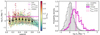 |
Fig. 5. Left panel: distribution in redshift of log Σ5. The contours show the density distribution of the points. The average values in different redshift bins are shown as black points. The black line shows the average log Σ5 for all the miniJPAS galaxies; and magenta and blue lines show the average log Σ5 for galaxies in groups and in the field environment, respectively. Dashed lines are at the average log Σ5 for galaxies with Passoc > 0.6 or 0.8. The colour bar shows the distribution of the rest-frame (u − r) colour. Vertical structures are groups in miniJPAS. Right panel: distribution of log Σ5 for miniJPAS galaxies (grey area) and field galaxies (grey line), and galaxies in a group (magenta) environment. Vertical lines show the positions of the average values. |
The local density is a proxy of the local environment, which is sensitive to the processes taking place on small scales (e.g., Calvi et al. 2018). It can be defined in different ways (e.g., Muldrew et al. 2012); for example, by counting galaxies within a fixed radius (such as 0.5 Mpc or 1.0 Mpc) or by measuring the distance to the Nth nearest neighbour (dN). Usually, N of between 3 and 5 is enough to characterise small scale environment, while N ∼ 10 is for large-scale and denser environment.
To characterise the local density of galaxies in miniJPAS, we use the environment indicator Σ5 (Lopes et al. 2016), which is defined as  and describes the local number density around a galaxy within an area defined by the projected area of the fifth nearest neighbour (d5) within a given redshift slice (Dressler 1980). With this definition, the local density is measured in units of galaxies per Mpc−2.
The distribution of log Σ5[Mpc−2] for the miniJPAS galaxy sample ranges from −1 to 2.5, with an average value of 0.1 (Fig. 5). This mean value is low, and lower than the local density expected for galaxies located in the centre of clusters log Σ5 [Mpc−2] ≥ 2 (see e.g., Lopes & Ribeiro 2020). The fraction of galaxies above log Σ5 [Mpc−2] ≥ 2 is small (< 0.2%), suggesting that certainly there are not too many high-overdensity structures, such as clusters, in miniJPAS. However, the galaxies in AMICO groups are tracing the local overdensity in miniJPAS, with an average value of log Σ5 [Mpc−2] equal to 0.67 (std = 0.52). We stress that the distribution of log Σ5 for galaxy group members changes very little with Passoc (see panel right in Fig. 5). The average of log Σ5 changes from 0.57 to 0.75 Mpc−2 when galaxies with Passoc larger than 0.6 or 0.8 are taken as galaxy members. Thus, the galaxy members of the AMICO groups are tracing intermediate densities, and they are very useful for studying the role that the group environmental conditions play in quenching the star formation in galaxies. It is also interesting to note that the BGGs of these groups are tracing a similar distribution of the local overdensity to the satellite galaxies, because they are found in the regions with higher contour densities (see right panel of Fig. 2), which also have an equal average value of log Σ5 of 0.64 (std = 0.53). On the other hand, the galaxies in the field have an average log Σ5 [Mpc−2] of 0.03 (std = 0.39), which is significantly lower than the average density of galaxies in groups. We note that there is some overlap between the log Σ5 [Mpc−2] distributions of the field and group populations (right panel in Fig. 5). There are field galaxies located in overdensity regions with log Σ5 [Mpc−2] > 0.5 and some galaxy group members in regions of log Σ5 [Mpc−2] < 0.
4. Stellar population properties of galaxies in groups
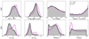 |
Fig. 6. Stellar population properties derived from the J-spectra (MAG_AUTO) fits with BaySeAGal for the whole miniJPAS sample (grey area and dashed black line), for galaxies in the field (black-line), and galaxies in a group environment (magenta line). From left to right, and from top to bottom: PDF of the galaxy stellar mass, mass-weighted age, stellar extinction, stellar metallicity, rest-frame (u − r) colour, extinction-corrected rest-frame (u − r) colour, and the parameters of the SFH: t0 and τ. |
Previous works have pointed out several divergent and/or contradictory results when the properties of galaxies are studied as a function of environment. For example, earlier SDSS works found that there is a correlation between galaxy colour, age, metallicity, and SFR with the environment density (e.g., Blanton et al. 2005). At a fixed stellar mass, both the star formation and the nuclear activity depend strongly on local density (Kauffmann et al. 2004). On the other hand, Blanton & Moustakas (2009) found that the position of the blue cloud and red sequence are independent of environment. The colour–mass and the colour-concentration indices do not vary strongly with environment (Baldry et al. 2006). Further, Bamford et al. (2009), using morphological classification from the Galaxy Zoo, conclude that morphology does not depend on environment once the colour of a galaxy is fixed. However, old galaxies are preferentially located in dense regions, and at a fixed Sersic index, the stellar population ages depend strongly on density (Baldry et al. 2006).
Thanks to the development of codes to find groups (e.g., Yang et al. 2007), galaxy properties have been studied by distinguishing between the satellite and central galaxy populations. For example, Pasquali et al. (2010) found that satellite galaxies are older and more metal-rich than central galaxies of the same stellar mass. Further, the slopes of the age–stellar mass and the metallicity–stellar mass relations become shallower in dense environments (Petropoulou et al. 2012). In contrast, more recent works using samples at higher redshift (z < 1) find that the differences between the properties of central and satellites populations are not significant (Sobral et al. 2022), although the transformation that drives the evolution of the overall galaxy population must occur at a rate that is two to four times higher in groups than outside of them (Kovač et al. 2010).
In this section, we present our comparison of the stellar population properties of the galaxies in groups with those that are in the field using miniJPAS. Our SED-fitting analysis allows us to derive in a consistent way the SFH parameters (τ and t0), SFR, sSFR, age, and metallicity of the stellar populations. We also derived the rest-frame galaxy colours corrected for dust extinction to segregate the galaxy populations into blue and intrinsically red galaxies and to study the variation of their properties as a function of group environment. Moreover, we discuss here the evolution of the stellar population properties of galaxy group members since z=1 in comparison with those of galaxies in the field.
4.1. Stellar population properties
To study the role of group environment in the evolution of galaxies, we first compared the stellar population properties of galaxies in groups (Passoc ≥ 0.7) and in the field (Passoc ≤ 0.1). Specifically, we compared the galaxy stellar mass, age, extinction, stellar metallicity, rest-frame colour, extinction-corrected rest-frame colour, the time of the onset of star formation, and the e-folding time (log M⋆, ⟨log age⟩M, AV, ⟨log Z⋆⟩M, (u − r)res, (u − r)int, t0, and τ, respectively). These properties were calculated using MAG_AUTO magnitudes.
The distributions of log M⋆, ⟨log age⟩M, (u − r)res, (u − r)int, t0, and τ for galaxies in groups and in the field are different; in contrast the distributions of AV and ⟨log Z⋆⟩M are similar (Fig. 6). Masses, ages, and colours of the group population are clearly shifted to higher values with respect to the field population, indicating that on average the galaxy populations in the group environment are more massive, redder, and older than in the field. There is a shift of 0.24 dex, 0.21 dex, 0.3 dex to higher log M⋆, ⟨log age⟩M, and to redder colours (Table 1). The distributions of the SFH parameters t0 and τ are significantly different. t0 is shifted to earlier epochs, and τ to lower values in groups. These are indicators that group galaxies started to form stars earlier and during a shorter period of time than the galaxies in the field. However, these results do not mean that the group galaxy populations are intrinsically more massive, redder, and older than the field population, and the results could be more a consequence of a large fraction of red, older, and massive galaxies in dense environments than in the field. We discuss this point further below.
Median and dispersion of the stellar population properties and SFH parameters of the red and blue galaxies in groups and in the field.
4.2. Identification of red and blue galaxies
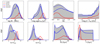 |
Fig. 7. PDF distributions for the stellar population properties of the galaxies in miniJPAS (grey area), and red (RG) and blue galaxy (BG) populations in a group environment (continuum red and blue lines), and galaxies in the field (dashed red and blue lines). |
To identify the red and blue galaxy populations in group and field environments, we used the method developed by Díaz-García et al. (2019a) using a sample of galaxies at z < 1 from the ALHAMBRA survey, which we adapted for the galaxy populations in miniJPAS (González Delgado et al. 2021). We classify galaxies as red or blue according to their extinction-corrected rest-frame (u − r)int, stellar mass, and redshift. We set a colour limit defined as:
 (2)
(2)
where z is the photo-z of the galaxy and log M⋆ is its stellar mass. If a galaxy has (u − r)int above this  , it is classified as red; otherwise, the galaxy is labelled as blue. We note that galaxies in the field and in groups are both classified as red or blue using the same criterion detailed in Eq. (2).
Figure 7 compares the PDF distributions of the stellar population properties of red and blue galaxies in group environments with the distributions of galaxies in the field. Although the maxima of the PDFs are different, the shape of the PDF of red galaxies in groups is very similar to the PDFs of galaxies in the field. The PDF of blue galaxies in groups is slightly shifted to higher masses, older ages, redder (u − r)res and (u − r)int colours, and lower τ values with respect to blue galaxies in the field. However, these shifts are very small, with a difference between the median values of ∼0.1 dex, 0.14 dex, 0.2 mag, 0.14 mag, 0.1 mag, and −0.1 dex for logM⋆, ⟨log age⟩M, (u − r)res, (u − r)int, AV, and ⟨log Z⋆⟩M, respectively (see Table 1).
For red galaxies, the shapes of PDFs are very similar, and there is not a significant shift between the median values of the properties with respect to the red galaxy population in the field. The most relevant difference is that the maximum of the PDF peak is higher for the red galaxies in groups. This is an indication that the fraction of red galaxies is larger in a group environment than in the field. This is a well-known result in galaxy cluster and group studies (Dressler 1980; Balogh et al. 2004, 2009). We discuss this point further in Sect. 5.
4.3. Specific star formation rate of miniJPAS galaxies
The dependence of the SFR and sSFR on environment has also been studied in the past. Kauffmann et al. (2004), for instance, found that sSFR is the most sensitive property to the local galaxy density. In contrast, other works suggest that the sSFR and its relation with the galaxy stellar mass of star forming galaxies is independent of environment up to z ∼ 1 (Peng et al. 2010; Darvish et al. 2016; Sobral et al. 2022). However, in very dense environments, a reduction in the SFR was found (Haines et al. 2013); although this reduction could be produced by the presence of a large fraction of red-disc galaxies with respect to less dense environment (Erfanianfar et al. 2016).
We calculated the SFR of each galaxy using the SFH derived from the fits by adding the mass gained during the last 100 Myr, and dividing this quantity by this period of time. This number is representative of the current SFR in the galaxy, and it is nearly equal to the SFR calculated using a period of time of ∼30 Myr, which is the epoch in which the galaxy optical luminosity is dominated by O and B0 stars, and the Hα line is detected in emission (Asari et al. 2007).
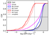 |
Fig. 8. Cumulative distribution of the specific SFR of the whole sample (light grey), the field galaxies (black line), the galaxy members of the AMICO groups (magenta), red galaxies in groups (dark red) and in the field (light red), and blue galaxies in groups (dark blue) and in the field (light blue). The vertical line shows the sSFR limit below which the galaxies are considered to be quenched. |
Figure 8 shows the cumulative distribution of sSFR values for galaxies in miniJPAS, and in the subsamples of galaxies in groups and in the field. Clearly, there is a difference of ∼ − 0.29 dex (median value) between the galaxies in groups and those in the field. Therefore, as pointed out by Kauffmann et al. (2004), sSFR is very sensitive to the environment, being lower in environments of high local density. However, this shift to lower sSFR is mainly due to the existence of a larger fraction of red galaxies in groups than in the field. The difference is smaller when the comparison is done considering the red and blue galaxy populations separately. The difference in the sSFR between galaxies in groups and in field is −0.16 and −0.13 dex for the blue and red populations, respectively. Therefore, we conclude that in the miniJPAS sample, the dependence of the sSFR on the group environment is small, ∼0.15 dex, when the red and blue galaxy populations are considered separately.
4.4. M⋆–sSFR relation in galaxies in groups
The star forming main sequence (SFMS) is the correlation between the SFR of a galaxy and its galaxy stellar mass. This relation is tight with a dispersion of only 0.2–0.3 dex at a fixed stellar mass and with a slope that is close to but below 1 (Brinchmann et al. 2004; Renzini & Peng 2015; Peng et al. 2010). There is also a tight relation between the intensity of the star formation and the stellar mass density of each galaxy region (González Delgado et al. 2016; Cano-Díaz et al. 2016), which defines a local SFMS, with a slope similar to the global galaxy SFMS. This suggests that local processes are relevant when determining the SFR in the disc of galaxies, probably through a density dependence of the SFR law (González Delgado et al. 2016). Recent results from the MaNGA survey confirm that the star formation in galaxies is governed by local processes within each spaxel (Bluck et al. 2020).
Nowadays, it is well-known that the star formation happening in the Universe since z ∼ 1 is mostly produced within blue galaxies, which in turn result in the SFMS (Brinchmann et al. 2004; Madau & Dickinson 2014), and the SFMS has existed since high redshift (Noeske et al. 2007; Elbaz et al. 2007; Whitaker et al. 2012; Tasca et al. 2015). A similar correlation exists between the sSFR and the galaxy stellar mass. Because the SFMS shows a slope of < 1, the sSFR declines weakly with increasing mass (Salim et al. 2007; Schiminovich et al. 2007).
Many previous works found that the SFMS is independent of environment (Peng et al. 2010; Darvish et al. 2015, 2016), and showed that the dependence of the SFR and the sSFR on the environment may be due to a larger fraction of quiescent galaxies in high-density environments. These latter authors suggest that environment does not regulate the build-up of mass in star forming galaxies.
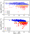 |
Fig. 9. log sSFR-log M⋆ relation for galaxies in the field (upper panel) and those in a group environment (bottom panel). Red and blue galaxies are represented by blue and red circles, respectively. Blue galaxies that are in a transition phase (see Sect. 6.3) are represented by orange circles. Black dashed lines represent the fit obtained for the SFMS in each set of galaxies. |
Figure 9 shows the relation between log sSFR and log M⋆ for galaxies in low-density environments and in groups. Blue (BG) and red galaxies (RG) are properly separated in the log sSFR and log M⋆ relation. As expected, BGs define the SFMS at a fixed stellar mass, while RGs are below this observational relation. To explore the dependence of the SFMS on environment, we fit a linear relation (log sSFR = b + a logM⋆) only to the star forming galaxies. Peng et al. (2010) proposed that only blue galaxies with sSFR > 0.1 Gyr−1 are actually star forming galaxies. Here, we exclude all the RGs and BGs that have sSFR below this threshold for fitting the SFMS. The results of the fit are (a, b)=(−0.23 ± 0.02, 2.0 ± 0.2) for galaxies in groups, and (a, b)=(−0.15 ± 0.01, 1.3 ± 0.1) for galaxies in the field. The differences between the SFMSs of star forming galaxies in groups and in the low-density environment are small, being negligible in the low-mass bins and ∼ − 0.18 dex in log sSFR for logM⋆ > 11. Thus, there is a reduction in star formation only in massive galaxies that are in a group environment with respect to the galaxies in less dense environments.
4.5. Mass–colour diagram versus environment
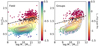 |
Fig. 10. Mass–colour (rest-frame (u − r) corrected for extinction) for the field galaxy population (left panel) and galaxies in a group environment (right panel). Dashed lines show the |

The bimodal colour distribution of galaxy populations is clearly seen in the (u − r)int–log M⋆ diagram (Fig. 10).The rest-frame colour corrected for extinction (e.g., (u − r)int) is more useful than (u − r)res for segregating the red and blue populations and for accounting for the fraction of red and star forming galaxies in the sample. The miniJPAS galaxies in the log M⋆–(u − r)int diagram are clearly distributed in the red sequence and the blue cloud, with the galaxies in the red sequence being typically old and metal rich (González Delgado et al. 2021). This mass–colour bimodal distribution is in place for the group and the field galaxy populations, although the fraction of galaxies that populate the red sequence and the blue cloud are different (Fig. 10).
It is well known that the bimodal colour distribution of galaxies is connected to the SFR and sSFR of galaxies, in the sense that blue galaxies have higher SFR and sSFR than red galaxies (Brinchmann et al. 2004; Salim et al. 2007; Renzini & Peng 2015; González Delgado et al. 2016, 2017; López Fernández et al. 2018). This result is clearly confirmed by our analysis in the AEGIS field in the colour (u − r)int–log M⋆ diagram (Fig. 10) for galaxies in the field and in groups. We stress that in both diagrams, red galaxies (located above the dashed line in Fig. 10) are redder than their (u − r)lim, which is calculated with Eq. (2) for each galaxy, and are characterised by a sSFR (SFR/M⋆) < 0.1 Gyr−1, whereas those in the blue cloud usually have sSFR > 0.1 Gyr−1.
Red colours and a sSFR below a given threshold are used as proxies for identifying quenched galaxies. Here, we find that the two proxies provide a similar fraction of quenched galaxies. Using sSFR < 0.1 Gyr−1 as a threshold, we find that 28% and 6% of the galaxies in groups and in the field are quenched, respectively. Using the (u − r)int colour–mass relation, the fraction of quenched galaxies is 23% and 5% in groups and in the field, respectively. Thus, the two proxies yield similar results, and indicate that there is on average a 20% excess of quenched galaxies in dense environments, in agreement with the findings of Balogh et al. (2009) who studied the fraction of red galaxies in groups at z ∼ 0.4. Furthermore, we find that on average the fraction of quenched galaxies is significantly higher in groups than in less dense environments, and it is also significantly higher than in the whole AEGIS galaxy population (lower than 8%). However, we note that this excess is a function of log M⋆ and redshift. We discuss this point further in Sect. 5.2.
4.6. Properties of the group central galaxies
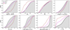 |
Fig. 11. Distribution of the properties of the central galaxy (brown line) compared with the properties of galaxies in groups (magenta line) and galaxies in the field (black line). From left to right, and top to bottom: stellar mass; absolute magnitude in the r band; intrinsic stellar extinction; stellar metallicity; rest-frame (u − r) colour; stellar age (mass-weighted); sSFR; and ratio of the SFH papameters t0 and τ. |
Here, we use the term central galaxies to refer to the most massive and brightest galaxies in each of the AMICO groups detected. As we explained in Sect. 3, these are the most massive galaxies close to the group centre. We now present our study of the stellar population properties of the BGGs (see Fig. 11), and show how we compare them with the properties of the other members of the groups, and with the sample of galaxies in the field environment. BGGs are significantly more massive (∼1 dex), brighter (∼1.6 mag), redder ((u − r)res ∼ 0.9 higher), older (⟨log age⟩M ∼ 0.9 dex higher), and more metal rich (⟨log Z⋆⟩M ∼ 0.4 dex higher) than the rest of the galaxy population in miniJPAS. BGGs are slightly less affected by extinction (AV ∼ 0.14 mag lower) than the rest of the galaxy sample. In terms of their star formation activity, BGGs are the galaxies with the lowest sSFR, ∼1 dex below the rest of the galaxy population in miniJPAS, suggesting that the star formation has been shut down significantly in these galaxies. Additional evidence of this shut down of the star formation taking place a long time ago and/or happening in a short period of time comes from τ/t0, which is very small (∼0.17) in comparison with the general miniJPAS galaxy population (τ/t0 ∼1.3). Differences between BGGs and the other group members are also significant, with the former being more massive, more luminous, more metal rich, older, and with lower sSFR than the rest of the galaxies in groups (see Table 1). The median values of sSFR, (u − r)res and τ/t0 suggest that BGGs are red quiescent galaxies; however, ∼38% of the BGGs are still forming stars with sSFR > 0.1 Gyr−1. However, this fraction decreases with redshift. Only ∼20% of the BGGs at z < 0.3 have sSFR > 0.1 Gyr−1; thus ∼80% are quiescent galaxies. This is in agreement with previous results from SDSS that show that 80% of the central galaxies in clusters at z < 0.1 have ceased their star formation independently of their stellar mass (von der Linden et al. 2010).
4.7. The evolution of the stellar population properties
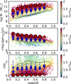 |
Fig. 12. Evolution of stellar mass, age, and the ratio of the SFH parameter τ/t0. The contours represent the density distribution of points. The dots represent the average values of each property in each redshift bin. Blue and red circles (stars) are the values for blue and red galaxies in group (field) environments. The dispersion with respect to the average is shown as error bars. |
The environment can play a different role at different epochs. Here, we explore the properties of the red and the blue populations in groups and in low-density environment as a function of redshift. In particular, we explore the evolution of log M⋆, ⟨log age⟩M, and τ/t0.
Previously, we discussed the evolution of the miniJPAS red and blue galaxy populations with redshift (González Delgado et al. 2021). We found that red and blue galaxies are properly distinguished by their stellar content and properties. At any redshift bin below z = 1, the red galaxies are older and redder than the blue galaxies; and both galaxy populations are ageing since z = 1. The red galaxies are also more massive than the blue population. The median of the stellar mass values in our sample is higher at z = 1 than at z = 0. However, this is a consequence of the incompleteness of the sample, because galaxies less massive than 1010 M⊙ are not detected at z > 0.8, and galaxies with 2 × 10⁸ M⊙ are detected only up to z = 0.15 (see Fig. 19 in González Delgado et al. 2021).This also applies to the actual sample.
Figure 12 shows the average values of the various galaxy properties in each redshift bin. Blue and red galaxies are properly distinguished by their stellar content at any redshift bin. The local density of galaxies does not play a relevant role in setting the average properties of the red galaxies, because galaxies in groups and in the field have, on average, equal log M⋆, ⟨log age⟩M, and τ/t0 at any epoch; and, a similar behaviour have the blue galaxies, although at any redshift, blue galaxies in groups are slightly more massive, and the star formation extends over a shorter period of time. It is worth mentioning that the small differences between blue galaxies in groups and those in the field are almost constant, and independent of the redshift, although they tend to increase at lower redshifts. This is an indication that there is a larger fraction of blue galaxies in the transition phase to be transformed into red galaxies in groups. We discuss this point in Sect. 6.3.
5. Fraction of red and blue galaxies versus environment
5.1. The colour-density relation in miniJPAS
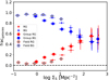 |
Fig. 13. Fraction of red and blue miniJPAS galaxies in different bins of log Σ5. The results for the whole galaxy sample (dots), galaxies in groups (red and blue circles), and in the field (grey-red and grey-blue circles) are shown. |
Large structures, such as galaxy clusters, have been extensively used to study the role that environment plays in galaxy evolution, in particular regarding the transformation of late-type to early-type galaxies, and how this depends on the local density number of galaxies. The pioneering work of Dressler (1980) revealed a clear morphology–density (T − Σ) relation, showing an increase in the fraction of early-type galaxies as a function of the local density number of galaxies.
The miniJPAS has proven to be a very successful survey for detecting clusters and groups with masses down to 1013 M⊙ (Maturi et al. in prep.). Here, we show that miniJPAS and our approach based on the bimodal colour distribution of galaxies is valid for studying the role that group environment plays in quenching the star formation in galaxies. Firstly, we show that our analysis can reproduce a relation similar to the morphology–density, T − Σ, relation by Dressler (1980), but using the blue–red colour classification of the sample instead of the morphology of the galaxy. This is justified because it is well known that the separation of the galaxy populations into red and blue galaxies in the colour–mass diagram is well correlated with the stellar population properties of the galaxies (Kauffmann et al. 2003a,b), and also with their morphology. In the local Universe, red galaxies are mainly elliptical- or spheroidal-dominated systems with little star formation, while blue galaxies are disc-dominated systems with ongoing star formation mostly concentrated in their spiral arms (Blanton & Moustakas 2009). On the other hand, previous works have confirmed a colour–density relation (e.g., Lewis et al. 2002; Kauffmann et al. 2004; Rojas et al. 2005; Weinmann et al. 2006; Liu et al. 2015; Moorman et al. 2016).
Figure 13 shows the fraction of red (fR) and blue (fB) galaxies in miniJPAS as a function of the local number density of galaxies measured by log Σ5. The error bars associated to fR and fB in each bin of log Σ5 are estimated as the confidence intervals of a binomial distribution. We use the normal approximation and a 68% confidence level. This distribution gives equal confidence intervals, and therefore errors, for fR and fB. These assumptions are also applied to calculate the error in Figs. 14–15. For figures in Sect. 6, the error bars are derived after propagation of the confidence intervals associated to the different fraction of galaxies involved in the calculation of the property shown in the figure.
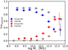 |
Fig. 14. Fraction of red and blue galaxies in different stellar mass bins for galaxies in groups (red and blue circles) and in the field (grey-red and grey-blue circles). The bins have a width of 0.4 dex in stellar mass and the points are plotted at the mean mass of the galaxies that belong to each bin. |
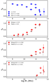 |
Fig. 15. Evolution of the fraction of blue and red galaxies as a function of galaxy stellar mass. Upper panel: fraction of blue galaxies in groups in three redshift bins, z < 0.3 (squares), 0.3 < z < 0.6 (cross), and 0.6 < z < 0.9 (stars). Bottom three panels: fraction of red galaxies in groups (red symbols) and in the field (grey-red symbols) for three redshift bins. |
We find that fR increases with log Σ5, while fB decreases. For example, fR increases from 0.04 at a value of log Σ5 [Mpc−2] = 0.02, which is more representative of a field environment, up to 0.2 when log Σ5 [Mpc−2] = 0.9, a value representative of groups. This increase is more significant, that is, up to ∼65%, when sampling the large structure of the AEGIS field, the cluster mJPC2470-1771 (Rodríguez Martín et al. 2022). It is worth noting that fR in groups is significantly higher than in the field for log Σ5 [Mpc−2] > 0; for example, fR is 0.36 for log Σ5 [Mpc−2] = 1.3, while it decreases down to zero for galaxies in the field. We can conclude that the colour–density relation in AEGIS is driven by the galaxy group population.
5.2. Fraction of red and blue galaxies in groups
This section discusses the impact of stellar mass and group environment on the quenching process. Broadly, two distinct scenarios have been proposed for quenching: mass quenching and environmental quenching. Peng et al. (2010) found that in the zCOSMOS sample (z ≤ 1) the effects of stellar mass and environment on the fraction of star forming and passive galaxies are separable. In contrast, other studies based on the CANDELS survey (Liu et al. 2021) have found that the quiescent fraction is relatively large at the high-mass end and at local environmental overdensities, which suggests a dependence of quenching on both mass and local environment.
Figure 14 shows fR and fB as a function of the galaxy stellar mass for the group and field subsamples. We note that these fractions, fR and fB, are not corrected by volume incompleteness of the sample. In González Delgado et al. (2021), we showed that galaxies with logM⋆ ∼ 10 can be detected up to z ∼ 0.8 in miniJPAS. However, at the highest redshift bin, we can calculate fR only for the bins of mass above 1011 M⊙.
Galaxies with logM⋆ ≤ 9 were not detected in groups, although they are in the field. For logM⋆ > 10, the fraction of red (blue) galaxies is significantly higher (lower) in groups than in the field. However, the differential effect is significantly higher for logM⋆ ≥ 11 than for lower masses. This suggests a dependence of quenching on both mass and group environment.
It is well-known that the fraction of blue galaxies in the core of galaxy clusters at intermediate redshift (z ∼ 1) is higher than in clusters at lower redshift (Butcher & Oemler 1984). To test this result in a less dense environment, we studied the evolution of galaxy populations in miniJPAS groups. We split the sample into three redshift bins (z ≤ 0.3, 0.3 < z ≤ 0.6, and 0.6 < z ≤ 0.9), and compared the fraction of red and blue galaxies in each of them. Figure 15 clearly shows that the fraction of blue galaxies in miniJPAS at a fixed log M⋆ is higher in the intermediate redshift bins than at z < 0.3. For example, for galaxies with (logM⋆ ∼ 10.6), fB is 50%, 92%, and 100% for z ≤ 0.3, 0.3 < z ≤ 0.6, and 0.6 < z ≤ 0.9, respectively. This result confirms the Butcher-Oemler effect in miniJPAS.
In agreement with these latter findings, the fraction of red galaxies (fR) in groups evolves with redshift, being higher at lower redshifts. To differentiate the effect of redshift and stellar mass, we compared fR in groups and in the field as a function of log M⋆. It is worth mentioning that the fraction of red galaxies detected in miniJPAS at 0.3 < z < 0.9 is small, fR ∼ 10%, and because of volume incompleteness of the sample, only galaxies with stellar mass above log M⋆ ∼8.8 at z = 0.3, and 9.9 at z = 0.7 are detected in miniJPAS (see Fig. 19 in González Delgado et al. 2021). We find that the evolution with redshift is significant. For instance, fR in groups and for logM⋆ ∼ 11 ranges from 0.9 at z < 0.3, to 0.36 at 0.3 < z ≤ 0.6, and 0.11 at 0.6 < z < 0.9. However, the increase in fR in groups with respect to the field ( ) does not vary significantly with redshift, where the mean and the standard deviation are ΔfR = 0.13 ± 0.06, 0.12 ± 0.11, and 0.14 ± 0.16 for the low, intermediate, and higher redshift bins, respectively. Further, the incremental effect of ΔfR is less dependent on the galaxy mass at z ≤ 0.3 than at z > 0.6. This is also in agreement with Liu et al. (2021) who find that the process of star formation quenching exhibits a strong dependence on stellar mass at early epochs, and the mass dependence of quenching tends to decrease with cosmic time.
6. Discussion
6.1. Fraction of quenched galaxies in groups
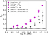 |
Fig. 16. Fraction of quenched galaxies in different stellar mass bins for galaxies in group environments and in the field. Different assumptions in Passoc are taken for selecting galaxies in groups: Passoc ≥ 0.7, Passoc ≥ 0.8, and Passoc ≥ 0.6 (magenta circles, dots, and stars, respectively); and galaxies in the field: Passoc < 0.1, Passoc < 0.1 and logΣ5 < 0, and Passoc < 0.1 and logΣ5 > 0 (grey circles, dots, and stars, respectively). |
In addition to colours, sSFR and SFR are also used to identify galaxies that have shut down their star formation (e.g., Peng et al. 2010; Bluck et al. 2019). These alternative proxies for quenching allow the selection of galaxies outside the SFMS, independently of their colour or morphology. Here, we follow the criterion in Peng et al. (2010), which considers that a galaxy is quenched when sSFR ≤ 0.1 Gyr−1. This results in an average fraction of quiescent galaxies (fQ) of 28% in groups and 6% in the field. These average values are similar to but slightly higher than the average fraction of red (fR) galaxies in groups (23%) and in the field (5%). The difference between the quenched and red fractions can be accounted for by the small fraction of blue galaxies with sSFR ≤ 0.1 Gyr−1.
Both fQ and fR change with log M⋆. Both show similar behaviour with log M⋆; although fQ is higher than fR in the highest mass bins. This is mainly due to a larger fraction of quenched galaxies in groups that still have blue colours, although fQ and fR are similar for massive galaxies in the field. This difference can be explained if there is a large fraction of post-starburst galaxies in dense environment with respect to the field, as found previously in clusters (Poggianti et al. 2009). Post-starburst galaxies shut their star formation down recently and rapidly, but they still have an intermediate age population dominating the optical colours.
To differentiate between the dependence of fQ with log M⋆ and with environment, Fig. 16 shows fQ versus log M⋆ (in 0.4 dex mass bins) for galaxies in groups and in the field. Although fQ increases with log M⋆ for galaxies more massive than 1010 M⊙, the increase is significantly higher for galaxies in groups than in the field. In groups, fQ ∼ 4%, 50%, and 80% for logM⋆ ∼ 10, ∼11, and ∼11.5; while in the field fQ ∼ 2%, 20%, and 55%.
To check the dependence of fQ on the criteria for group membership, we calculate fQ after changing the threshold value of Passoc. The results indicate that fQ in groups varies only a little when P > 0.7 is changed to Passoc > 0.8 or Passoc > 0.6. Moreover, fQ goes from 79% to 71% for galaxies with logM⋆ = 11.4, which are the galaxies for which the difference in fQ is higher. However, the variation of fQ with the criteria to select galaxies in the field is more significant (Fig. 16). Here, we compare the results obtained with the following criteria: (i) Passoc < 0.1; (ii) Passoc < 0.1, and logΣ5 < 0; (iii) Passoc < 0.1 and logΣ5 > 0. Although fQ is independent of the field definition for low-mass galaxies, fQ changes significantly for the galaxies more massive than logM⋆ > 11. Thus, fQ varies from 25% to 53% in the field at logM⋆ = 11.4. However, in each bin of galaxy stellar mass, the upper limit fQ in the field sample is still significantly below fQ in groups. Thus, independently of the galaxy field selection, and the galaxy group population, fQ is always higher in groups.
6.2. Fraction excess of quenched galaxies
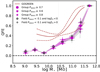 |
Fig. 17. Quenched fraction excess in different bins of stellar mass. Different symbols are the QFE measurements derived using the different assumptions to select galaxy members of groups, or galaxies in the field as in Fig. 16. The brown curve is taken from McNab et al. (2021), the QFE inferred from the Schechter function fits to the GOGREEN data. The dashed lines represent their 68% confidence interval. |
The most important characteristic of the galaxy populations in groups with respect to less dense environments is the large fraction of red galaxies. This characteristic is related to a larger fraction of galaxies in groups that have quenched their star formation with respect to galaxies in the field. This difference can be measured by the quenched fraction excess (QFE). Here we adopt the definition given by McNab et al. (2021) in their Eq. (4):
 (3)
(3)
where  and
and  are the fractions of star forming galaxies in the field and in groups, respectively. We note that a larger fraction of quenched galaxies is equivalent to a lack of star forming galaxies in groups with respect to low-density environments. QFE represents the fraction of field star forming galaxies that need to be quenched at the epoch of observation to be equal to the quenched population in groups. This measures the quenching that can be attributed to the group environments. This definition is equivalent to the environmental quenching efficiency defined by Peng et al. (2010), Wetzel et al. (2015), Nantais et al. (2017), and van der Burg et al. (2018), the transition fraction by van den Bosch et al. (2008), and the conversion fraction by Balogh et al. (2016), and Fossati et al. (2017).
Here, we present our study of the behaviour of QFE in response to varying M⋆ (Fig. 17). QFE increases with M⋆ for galaxies above 1010 M⊙, and is smaller than ∼10% for galaxies less massive than 1010 M⊙ and is negligible below 109 M⊙. This behaviour is independent of the definition of field and the value of Passoc to select galaxy members in groups. For example, for galaxies of 1010–1011 M⊙, QFE changes by < 5%, when galaxy members of the groups are selected with Passoc > 0.6 or greater than 0.8 instead of 0.7. A similar effect is produced when only galaxies with Σ5 > 1 Mpc−2 or below this density are included in the sample of field galaxies, as well as Passoc < 0.1. A larger effect is found for mass bins higher than 1011 M⊙. In this range, QFE increases from 0.48 to 0.67 by changing the field definition.
The relation between QFE and M⋆ found in our work is similar to that derived for high-density environments (Balogh et al. 2016; van der Burg et al. 2020; McNab et al. 2021). However, we find relevant differences with respect to cluster environments (McNab et al. 2021; van der Burg et al. 2020). For example, in the GOGREEN survey (Balogh et al. 2017), which measures the rate of environmentally driven star formation quenching in clusters at z ∼ 1, QFE is constant at ∼0.4 for logM⋆ < 10.5 (McNab et al. 2021; van der Burg et al. 2020); while we find that QFE in group environments is significantly smaller (≤0.1) for galaxies with 1010 M⊙. For more massive galaxies in clusters, QFE increases up to ∼1 for galaxies of logM⋆ = 11.5; while in AEGIS groups, QFE increases with stellar mass but only up to 0.6 for logM⋆ = 11.5, and rises to 0.4 for logM⋆ = 11. It is interesting to note that QFE ∼ 0.4 is the value derived by Peng et al. (2012) for low-redshift satellite galaxies; and is the value that we derive for galaxies of 1011 M⊙.
6.3. Fraction excess of transition galaxies
It is interesting to identify galaxies that are in a transition phase between the blue cloud and the red sequence because this population provides clues as to the rate of environmental quenching. Post-starburst galaxies, blue quiescent galaxies, red spirals, and green valley galaxies (Poggianti et al. 1999; Tojeiro et al. 2013; Schawinski et al. 2014; Lopes et al. 2016) form part of these transition galaxy populations.
First, we identified blue quiescent galaxies as those galaxies classified as blue by their colour in the (u − r)int–log M⋆ plane and with sSFR < 0.1 Gyr−1. They are below the SFMS (see Fig. 9) and are expected to be galaxies in a transition phase between the blue cloud and the red sequence. Furthermore, in the colour (u − r)int–log M⋆ diagram they are located in the area just below the red sequence (see Fig. 10), where the so-called green valley is located (Schawinski et al. 2014). The fraction of these galaxies in miniJPAS is small (2.3%), but is significantly larger in the group environments (6.7%) than in the field (1.8%). The fraction excess of these galaxies, defined as the difference between the fraction of transition galaxies in groups with respect to those in the field,  , is not constant with M⋆. Although uncertainties are large due to the small number of transition galaxies in each bin of galaxy stellar mass, we find that the differential fraction (Δfi) is equal to zero for galaxies with logM⋆ ≥ 11, but increases from 5% to 9% for galaxies with masses between 1010.5 and 109 M⊙. These results are consistent with those obtained by McNab et al. (2021) for the galaxy members of clusters from the GOGREEN survey, where
  for the blue quiescent galaxy population increases to lower galaxy masses up to ∼10%.
Instead of colours and sSFR, some studies use the relative position of the galaxy with respect to the SFMS to identify green valley objects. Here we use the Bluck et al. (2020) definition, where green-transition galaxies are those that for a given mass bin have a variation with respect to the SFMS, ΔSFR (logSFR – logSFRMS), between −0.5 and −1 dex. Using this definition and the SFMS law for star forming galaxies in groups and in the field derived in Sect. 4.4, we identify this transition galaxy population. The fraction of this transition population and its behaviour with log M⋆ is similar to that derived for the blue quiescent population. Further, both criteria to identify the transition galaxy population provide a value of  that is compatible with the results derived in the GOGREEN survey (McNab et al. 2021).
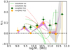 |
Fig. 18. Riτi as a function of galaxy stellar mass, calculated from Eq. (4). Orange points represent the values obtained using the colour–sSFR definition for the transition galaxies (TG2). Green points represent the values obtained using the Δ SFR definition for transition galaxies (TG1). The magenta and grey shades correspond to the different assumptions on Passoc for the group members and field galaxies, respectively. Light green and coral lines are the results from McNab et al. (2021) for the green and blue quiescent galaxy populations in GOGREEN. Dashed lines (same colours) represent the 68% confidence limits of their fit. |
The excess in the abundance of transition galaxies is related to the rate of the environmental quenching and the time spent in that phase. If Ri is the fraction of field star forming galaxies that are quenched per unit of time as they are falling into the group, and τi the time spent in the transition phase, the relative abundance excess of transition galaxies is:
 (4)
(4)
As pointed out by McNab et al. (2021), this equation requires several assumptions: (i) the mass accretion rate is constant with time; (ii) the abundance excess of transition galaxies is produced only by quenching; (iii) the number of transition galaxies attributable to non-environmental effects is proportional to the total galaxy population.
Figure 18 shows Riτi as a function of the stellar mass calculated with Eq. (4) assuming different definitions of the galaxies in groups and in the field. Passoc changes from 0.6 to 0.8, and galaxies with Passoc < 0.1 and logΣ5 > 0 or < 0 are selected to belong to the field. As explained above, we use different assumptions for selecting transition galaxies based on the sSFR and (u − r)int colour (magenta and grey points), or by ΔSFR with respect to the MSSF (green points). It is difficult to estimate Riτi for galaxies with masses larger than 1011 M⊙. The value of Riτi shows differences depending on whether we select the transition galaxies according to the green valley or the blue quiescent galaxies. For mass bins lower than 1011 M⊙, Riτi is only weakly dependent on the field or galaxy group member selection, and on the transition galaxy population definition. There is an increase in Riτi with decreasing mass, with a maximum of Riτi ∼ 0.1 at 1010.5 M⊙, and a plateau of 0.05 for lower masses. These findings are compatible with those of McNab et al. (2021) for the GOGREEN survey. However, the results of these latter authors show an increase in Riτi with decreasing mass, and the mass threshold for Riτi > 0 is 1011 M⊙ for the blue quiescent galaxies and 1010.5 M⊙ for the green valley populations. It is worth pointing out that the 68% confidence limits in Riτi for the GOGREEN survey are compatible with the maximum Riτi at 1010.5 M⊙ in miniJPAS, and the lack of constraint in the most massive galaxies of the sample.
6.4. Transition timescales
To infer the rate of environmental quenching Ri, we need to know the time that the transition galaxies spend in this phase, τi. Some authors have suggested that τi ∼ 0.5 Gyr, in particular for post-starburst and blue quiescent galaxies (Belli et al. 2019; Muzzin et al. 2014). In other works, τi is equivalent to the time that the galaxy spends fading its star formation (tfade). In particular, Balogh et al. (2016) estimated tfade = 0.5 ± 0.2 Gyr for clusters and 0.9 ± 0.3 Gyr for groups from the surveys at 0.8 < z < 1.2.
Here, we calculate τi as the fading timescale (tfade), which is related to the relative abundance of the transition galaxies with respect to the star-forming galaxy population (Balogh et al. 2016). Thus,
 (5)
(5)
where tSF + trans is the time during which all the presently star forming and transition satellite galaxies fall into the cluster, and can be approximated to the lifetime (T) of the cluster at a given epoch, which is also equivalent to the total quenching timescale (tq).
Balogh et al. (2016), using the Millennium simulations (Springel 2005), and assuming that QFE evolves similarly to the fraction of halo mass assembled, find that tq evolves similarly to the dynamical time as A × (1 + z)−3/2, where A is the lookback time when the halo started to assemble satellites, and has a small dependence on the halo mass. Assuming that our AMICO groups have a halo mass of several times 1013 M⊙, we derive T = tq ∼ 6.5 Gyr for the mean redshift (z = 0.39) of our transition galaxies; and τi = tfade ∼ 0.8 Gyr and 1.5 Gyr if colour and sSFR (TG1) or ΔSFR (TG2) are used to select the transition galaxy population in miniJPAS. These values are in agreement with the average tfade derived by Balogh et al. (2016) for groups in a similar range of redshift.
6.5. The evolution of group galaxy quenching
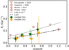 |
Fig. 19. Rate of group galaxy quenching in four redshift intervals for miniJPAS. The rate is calculated using two proxies for selecting transition galaxies (orange and green points). Results from Fig. 15 in McNab et al. (2021) are shown (grey-red points). The dashed line is QFE/T for QFE = 0.4, and the dotted line represents the evolution of the inverse of the dynamical time, (1 + z)3/2 scaled to R = 0.05 Gyr−1 at z = 0 (see the text for further explanation). |
To explore the evolution of the group galaxy quenching rate, we divided the group sample into four redshift bins from 0.05 to 0.85 with a width of 0.2. First, we derived T (tq) for the mean redshift within each bin, and τi (tfade) using Eq. (5) for each redshift interval. Then, we derived the evolution of the rate of the group galaxy quenching from Eq. (4) and τi in the four redshift bins (Fig. 19). Further, we calculated T (tq), τi (tfade) and Ri for the two proxies used to define transition galaxies: blue colour and sSFR < 0.1 Gyr−1 (blue quiescent galaxies, magenta points) or −1 < ΔSFR < −0.5 dex (green valley, green points). It is remarkable that both proxies provide similar results for the group galaxy quenching rate (R) within the uncertainties, which are compatible with a modest but significant evolution in R from z ∼ 0.8 to 0.2. This evolution is compatible with the expected evolution by a constant QFE = 0.4; R = QFE/T with T being the lifetime of a cluster formed at z = 3 at each given epoch (dashed line in Fig. 19). This line also connects with the quenching rate R derived for GOGREEN clusters at z = 1.2 (grey-yellow cross) from McNab et al. (2021). Other results from Paccagnella et al. (2019), Poggianti et al. (2009), and Muzzin et al. (2012) as adapted from McNab et al. (2021) are shown in Fig. 19. The evolution of the inverse of the dynamical time, (1 + z)3/2, scaled to R = 0.05 Gyr−1 at z = 0 is also plotted. Although our uncertainties are large, in particular at the two highest redshift bins, R is below this evolutionary line. We therefore conclude that the rate of group quenching shows a modest evolution that is compatible with a simple model in which QFE is constant and equal to 0.4 at z ∼ 0. On the other hand, QFE is equal to 0.4 at 0.05 < z < 0.25 in the miniJPAS groups.
6.6. The efficiency of group galaxy quenching
Our results suggest that galaxy quenching is less efficient in group environments than in cluster environments, given that QFE is about a factor of two lower in the AEGIS groups than in clusters, at least for M⋆ < 1011 M⊙ (see Fig. 17). This is expected from the IllustrisTNG simulations, which show that the quenched fraction increases with virial mass, M200 (Donnari et al. 2021a,b). These latter authors found that the fraction of galaxies with M⋆ ∼ 1010 M⊙ that are quenched at z = 0 increases from fQ = 0.2 to 0.7 if they belong to halos of M200∼1013 M⊙ to 1014 M⊙. In contrast, fQ ∼ 0.9 independently of M⋆ in very massive halos (> 1014 M⊙) (Donnari et al. 2021a).
To compare the efficiency of groups with respect to clusters, Fig. 20 compares the QFE derived from the smaller groups in our sample (Mgroup < 5 × 10¹¹ M⊙) with respect to the most massive structure found by AMICO in miniJPAS, the cluster mJP2470-1771 (Bonoli et al. 2021). A very detailed analysis of the spatial distribution of galaxy populations (quenched star forming galaxies and AGNs) is presented in Rodríguez Martín et al. (2022). Its halo mass is M200 = 3.3 × 10¹⁴ M⊙. From our own analysis presented here, we estimate that this cluster is about ten times more massive than the most massive group considered in Fig. 20. We find that QFE is about a factor of two higher in this cluster than in AMICO small groups, and is in agreement with what is expected from the IllustrisTNG simulations.
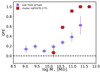 |
Fig. 20. Quenched fraction excess derived using the less massive groups (Mgroup < 5 × 10¹¹ M⊙) and for the most massive density structure in the miniJPAS survey, the cluster mJP2470-1771. |
From this limited analysis, we can conclude that quenching, for galaxies with M⋆ > 1010 M⊙, is less efficient in small groups than in clusters. Small groups also seem to be less favourable environments for quenching of galaxies with M⋆ < 1010 M⊙. A deeper potential well associated to the cluster stimulates galaxy interactions and mergers and tidal stripping; higher galaxy number density favours harassment; and higher ambient gas density is advantageous to ram-pressure stripping processes. These processes do that galaxies can be quenched after being accreted into the cluster host. Further, galaxies can also be quenched while they are members of pre-processing group hosts that are also accreted to the cluster.
7. Summary and conclusions
The goal of this paper is to illustrate the power of J-PAS to investigate the role that environment plays in galaxy evolution. In particular, the role of group environment in quenching star formation in galaxies, and its evolution since z ∼ 1. First, we analysed the stellar population properties of galaxies with M⋆ ≥ 109 M⊙ that belong to a sample of 80 groups with M200 down to 1013 M⊙ detected by AMICO in miniJPAS. Galaxy members of the groups were selected based on the association probability from AMICO, Passoc ≥ 0.7. A subsample of galaxies of miniJPAS representative of a low number density field (Passoc < 0.1) was also selected. Using the parametric SED-fitting code BaySeAGal, we derived the star formation history and the stellar population properties of the galaxies that belong to groups or to the field. In particular, we used the extinction-corrected rest-frame colour (u − r)int, M⋆, and sSFR for the identification of galaxies that have shut down their star formation. We measured the abundance of the red and blue galaxy populations, and the transition galaxies that are in a phase between the blue cloud and the red sequence as a function of the galaxy stellar mass in groups and in the field. Uncertainties associated to the criteria for the selection of galaxies as a function of the environment density were also studied. The main conclusions of our study can be summarised as follows:
-
Stellar population properties: Galaxies in groups are slightly older, redder, more metal-rich, and have lower sSFR and smaller τ/t0 values than galaxies in the field. However, the red galaxy population in groups has similar properties to that of the equivalent galaxy population in the field. Further, the evolution of the properties since z ∼ 1 is similar for the group and field galaxy populations.
-
BGG: The central (brighest) galaxy (BGG) is the most massive galaxy of the group. These galaxies are among the oldest, reddest, and most metal-rich objects of the red galaxy population. They have on average sSFR below 0.1 Gyr−1, and τ/t0 = 0.17 ± 0.34, indicating that star formation has already shut down, as in most of the red galaxy populations in groups and in the field.
-
Abundance of red galaxies: The fraction of red galaxies in miniJPAS increases with galaxy stellar mass; although this fraction is always higher in groups than in the field for galaxies more massive than 1010 M⊙. The fraction of blue galaxies decreases as the galaxy mass increases, and evolves as expected with redshift, being lower at z ∼ 0.1 than at z ∼ 0.8.
-
Fraction of quenched galaxies: 28% of the group galaxy population has sSFR ≤ 0.1 Gyr−1. This fraction is almost independent of the threshold value of Passoc used to define the galaxy group members. In contrast, the fraction of quenched galaxies in the field is only 5%, and it shows a dependence on the field galaxy population selected for the galaxies more massive than 1011 M⊙.
-
Quenched fraction excess: The QFE shows a strong dependence on galaxy stellar mass above 1010 M⊙, increasing from a few percent for M⋆ < 1010 M⊙, to 40% for 1011 M⊙, and 60% for 1011.5 M⊙.
-
Transition galaxies: Blue quiescent and green valley galaxies are identified as transition galaxy populations based on their colours, sSFR, or their SFR offset with respect to the main sequence of the star forming galaxies in groups and in the field. The fraction of transition galaxies is higher in the group environment than in the field.
-
Riτi: The abundance excess of transition galaxies relative to the star forming galaxy population (Riτi) shows a slight dependence on galaxy stellar mass, and is found to be between 5% and 10% for galaxies less massive than 1011 M⊙.
-
Transition timescale: The transition timescale is defined as the fading timescale (tfade = τi). It depends on the abundance of transition galaxies relative to that of star forming galaxies and the time since the transition and star forming galaxies were accreted to form the group. We obtain a mean value for tfade ∼ 0.8 Gyr for blue quiescent galaxies and ∼1.5 Gyr for the green valley galaxies.
-
The evolution of galaxy quenching rate: We find that Ri shows a modest but significant evolution since z ∼ 0.8. This evolution is compatible with the expected evolution, which follows a constant QFE = 0.4, and is in agreement with the expected evolution for clusters at z = 1.
These results show the potential of J-PAS in constraining the role that groups and clusters play in galaxy evolution. This potential resides in the accurate photo-z estimations (Hernán-Caballero et al. 2021) that allow us to identify groups and clusters up to z < 1 and to produce unbiased and complete mass-sensitive catalogues. Further, the J-spectra allow us to retrieve stellar population properties for the blue and red galaxy populations with a precision similar to future spectroscopic surveys with similar S/N, as demonstrated in González Delgado et al. (2021). Volume-complete samples can be studied above log(M⋆/M⊙)∼8.9, 9.5, and 9.9 at z = 0.3, z = 0.5, and z = 0.7, respectively.
Based on the whole sample analysed here, we expect that J-PAS will detect more than 90 million galaxies with r < 22.75 AB for which the stellar population properties will be derived. This is more than a factor 20 more than the whole SDSS survey (approximately 4.3 million galaxy spectra over the same area), and nearly a factor 3 more than the number of galaxies that will be observed by the Dark Energy Spectroscopic Instrument (DESI) survey (33 million galaxies over 14 000 deg2). In addition, more than 0.6 million groups and clusters will be detected (Maturi et al., in prep.), and it will be possible to disentangle the quenching due to halo mass from that caused by the environment in a wide range of galaxy stellar mass, groups, cluster properties, and evolution since z ∼ 1.
Star Formation History.
Star Formation Rate.
Acknowledgments
R.G.D., L.A.D.G., R.G.B., G.M.S., J.R.M., and E.P. acknowledge financial support from the State Agency for Research of the Spanish MCIU through the ‘Center of Excellence Severo Ochoa’ award to the Instituto de Astrofísica de Andalucía (SEV-2017-0709), and to PID2019-109067-GB100. I.M. acknowledges to PID2019-106027GB-C41. S.B. acknowledges to PGC2018-097585- B-C22, MINECO/FEDER, UE of the Spanish Ministerio de Economia, Industria y Competitividad. L.S.J. acknowledges the support from CNPq (304819/2017-4) and FAPESP (2019/10923-5). Based on observations made with the JST/T250 telescope and the Pathfinder camera for the miniJPAS project at the Observatorio Astrofísico de Javalambre (OAJ), in Teruel, owned, managed, and operated by the Centro de Estudios de Física del Cosmos de Aragón (CEFCA). We acknowledge the OAJ Data Processing and Archiving Unit (UPAD) for reducing and calibrating the OAJ data used in this work. Funding for OAJ, UPAD, and CEFCA has been provided by the Governments of Spain and Aragón through the Fondo de Inversiones de Teruel; the Aragón Government through the Research Groups E96, E103, and E16_17R; the Spanish Ministry of Science, Innovation and Universities (MCIU/AEI/FEDER, UE) with grant PGC2018-097585-B-C21; the Spanish Ministry of Economy and Competitiveness (MINECO/FEDER, UE) under AYA2015-66211-C2-1-P, AYA2015-66211-C2-2, AYA2012-30789, and ICTS-2009-14; and European FEDER funding (FCDD10-4E-867, FCDD13-4E-2685). J.A.F.O. acknowledges the financial support from the Spanish Ministry of Science and Innovation and the European Union – NextGenerationEU through the Recovery and Resilience Facility project ICTS-MRR-2021-03-CEFCA.
References
- Abadi, M. G., Moore, B., & Bower, R. G. 1999, MNRAS, 308, 947 [Google Scholar]
- Arnouts, S., Cristiani, S., Moscardini, L., et al. 1999, MNRAS, 310, 540 [Google Scholar]
- Asari, N. V., Cid Fernandes, R., Stasińska, G., et al. 2007, MNRAS, 381, 263 [Google Scholar]
- Baldry, I. K., Glazebrook, K., Brinkmann, J., et al. 2004, ApJ, 600, 681 [Google Scholar]
- Baldry, I. K., Balogh, M. L., Bower, R. G., et al. 2006, MNRAS, 373, 469 [Google Scholar]
- Balogh, M. L., Baldry, I. K., Nichol, R., et al. 2004, ApJ, 615, L101 [Google Scholar]
- Balogh, M. L., McGee, S. L., Wilman, D., et al. 2009, MNRAS, 398, 754 [CrossRef] [Google Scholar]
- Balogh, M. L., McGee, S. L., Mok, A., et al. 2016, MNRAS, 456, 4364 [NASA ADS] [CrossRef] [Google Scholar]
- Balogh, M. L., Gilbank, D. G., Muzzin, A., et al. 2017, MNRAS, 470, 4168 [NASA ADS] [CrossRef] [Google Scholar]
- Bamford, S. P., Nichol, R. C., Baldry, I. K., et al. 2009, MNRAS, 393, 1324 [NASA ADS] [CrossRef] [Google Scholar]
- Baqui, P. O., Marra, V., Casarini, L., et al. 2021, A&A, 645, A87 [EDP Sciences] [Google Scholar]
- Behroozi, P. S., Wechsler, R. H., & Conroy, C. 2013, ApJ, 770, 57 [NASA ADS] [CrossRef] [Google Scholar]
- Behroozi, P., Wechsler, R. H., Hearin, A. P., & Conroy, C. 2019, MNRAS, 488, 3143 [NASA ADS] [CrossRef] [Google Scholar]
- Bekki, K. 1999, ApJ, 510, L15 [NASA ADS] [CrossRef] [Google Scholar]
- Bell, E. F., Wolf, C., Meisenheimer, K., et al. 2004, ApJ, 608, 752 [NASA ADS] [CrossRef] [Google Scholar]
- Bellagamba, F., Roncarelli, M., Maturi, M., & Moscardini, L. 2018, MNRAS, 473, 5221 [NASA ADS] [CrossRef] [Google Scholar]
- Belli, S., Newman, A. B., & Ellis, R. S. 2019, ApJ, 874, 17 [Google Scholar]
- Benítez, N., Dupke, R., Moles, M., et al. 2014, ArXiv e-prints [arXiv:1403.5237] [Google Scholar]
- Benítez, N., Gaztañaga, E., Miquel, R., et al. 2009, ApJ, 691, 241 [Google Scholar]
- Blanton, M. R., & Moustakas, J. 2009, ARA&A, 47, 159 [Google Scholar]
- Blanton, M. R., Eisenstein, D., Hogg, D. W., Schlegel, D. J., & Brinkmann, J. 2005, ApJ, 629, 143 [Google Scholar]
- Bluck, A. F. L., Bottrell, C., Teimoorinia, H., et al. 2019, MNRAS, 485, 666 [Google Scholar]
- Bluck, A. F. L., Maiolino, R., Piotrowska, J. M., et al. 2020, MNRAS, 499, 230 [NASA ADS] [CrossRef] [Google Scholar]
- Bonoli, S., Marín-Franch, A., Varela, J., et al. 2021, A&A, 653, A31 [NASA ADS] [CrossRef] [EDP Sciences] [Google Scholar]
- Brinchmann, J., Charlot, S., White, S. D. M., et al. 2004, MNRAS, 351, 1151 [Google Scholar]
- Bruzual, G., & Charlot, S. 2003, MNRAS, 344, 1000 [NASA ADS] [CrossRef] [Google Scholar]
- Butcher, H., & Oemler, A. J. 1984, ApJ, 285, 426 [NASA ADS] [CrossRef] [Google Scholar]
- Calvi, R., Vulcani, B., Poggianti, B. M., et al. 2018, MNRAS, 481, 3456 [NASA ADS] [CrossRef] [Google Scholar]
- Cano-Díaz, M., Sánchez, S. F., Zibetti, S., et al. 2016, ApJ, 821, L26 [Google Scholar]
- Cappellari, M. 2016, ARA&A, 54, 597 [Google Scholar]
- Cenarro, A. J., Moles, M., Marín-Franch, A., et al. 2014, in Observatory Operations: Strategies, Processes, and Systems V, SPIE Conf. Ser., 9149, 91491I [NASA ADS] [Google Scholar]
- Cenarro, A. J., Moles, M., Cristóbal-Hornillos, D., et al. 2019, A&A, 622, A176 [NASA ADS] [CrossRef] [EDP Sciences] [Google Scholar]
- Chabrier, G. 2003, PASP, 115, 763 [Google Scholar]
- Chen, Y., Bressan, A., Girardi, L., et al. 2015, MNRAS, 452, 1068 [Google Scholar]
- Cid Fernandes, R., Mateus, A., Sodré, L., Stasińska, G., & Gomes, J. M. 2005, MNRAS, 358, 363 [Google Scholar]
- Cowie, L. L., & Songaila, A. 1977, Nature, 266, 501 [Google Scholar]
- Cristóbal-Hornillos, D., Varela, J., Ederoclite, A., et al. 2014, in Software and Cyberinfrastructure for Astronomy III, eds. G. Chiozzi, & N. M. Radziwill, SPIE Conf. Ser., 9152, 91520O [CrossRef] [Google Scholar]
- Darvish, B., Mobasher, B., Sobral, D., Scoville, N., & Aragon-Calvo, M. 2015, ApJ, 805, 121 [NASA ADS] [CrossRef] [Google Scholar]
- Darvish, B., Mobasher, B., Sobral, D., et al. 2016, ApJ, 825, 113 [NASA ADS] [CrossRef] [Google Scholar]
- Dekel, A., & Birnboim, Y. 2006, MNRAS, 368, 2 [NASA ADS] [CrossRef] [Google Scholar]
- Díaz-García, L. A., Cenarro, A. J., López-Sanjuan, C., et al. 2015, A&A, 582, A14 [Google Scholar]
- Díaz-García, L. A., Cenarro, A. J., López-Sanjuan, C., et al. 2019a, A&A, 631, A156 [Google Scholar]
- Díaz-García, L. A., Cenarro, A. J., López-Sanjuan, C., et al. 2019b, A&A, 631, A157 [Google Scholar]
- Díaz-García, L. A., Cenarro, A. J., López-Sanjuan, C., et al. 2019c, A&A, 631, A158 [Google Scholar]
- Donnari, M., Pillepich, A., Joshi, G. D., et al. 2021a, MNRAS, 500, 4004 [Google Scholar]
- Donnari, M., Pillepich, A., Nelson, D., et al. 2021b, MNRAS, 506, 4760 [NASA ADS] [CrossRef] [Google Scholar]
- Dressler, A. 1980, ApJ, 236, 351 [Google Scholar]
- Elbaz, D., Daddi, E., Le Borgne, D., et al. 2007, A&A, 468, 33 [NASA ADS] [CrossRef] [EDP Sciences] [Google Scholar]
- Erfanianfar, G., Popesso, P., Finoguenov, A., et al. 2016, MNRAS, 455, 2839 [NASA ADS] [CrossRef] [Google Scholar]
- Faber, S. M., Willmer, C. N. A., Wolf, C., et al. 2007, ApJ, 665, 265 [Google Scholar]
- Falcón-Barroso, J., Sánchez-Blázquez, P., Vazdekis, A., et al. 2011, A&A, 532, A95 [Google Scholar]
- Fossati, M., Wilman, D. J., Mendel, J. T., et al. 2017, ApJ, 835, 153 [Google Scholar]
- Gallazzi, A., Charlot, S., Brinchmann, J., White, S. D. M., & Tremonti, C. A. 2005, MNRAS, 362, 41 [Google Scholar]
- González Delgado, R. M., Pérez, E., Cid Fernand es, R., et al. 2014, A&A, 562, A47 [CrossRef] [EDP Sciences] [Google Scholar]
- González Delgado, R. M., Cid Fernandes, R., Pérez, E., et al. 2016, A&A, 590, A44 [NASA ADS] [CrossRef] [EDP Sciences] [Google Scholar]
- González Delgado, R. M., Pérez, E., Cid Fernandes, R., et al. 2017, A&A, 607, A128 [NASA ADS] [CrossRef] [EDP Sciences] [Google Scholar]
- González Delgado, R. M., Díaz-García, L. A., de Amorim, A., et al. 2021, A&A, 649, A79 [Google Scholar]
- Haines, C. P., Pereira, M. J., Smith, G. P., et al. 2013, ApJ, 775, 126 [NASA ADS] [CrossRef] [Google Scholar]
- Hayashi, M., Tanaka, M., Shimakawa, R., et al. 2018, PASJ, 70, S17 [NASA ADS] [Google Scholar]
- Hernán-Caballero, A., Alonso-Herrero, A., Pérez-González, P. G., et al. 2013, MNRAS, 434, 2136 [Google Scholar]
- Hernán-Caballero, A., Varela, J., López-Sanjuan, C., et al. 2021, A&A, 654, A101 [NASA ADS] [CrossRef] [EDP Sciences] [Google Scholar]
- Ilbert, O., McCracken, H. J., Le Fèvre, O., et al. 2013, A&A, 556, A55 [NASA ADS] [CrossRef] [EDP Sciences] [Google Scholar]
- Jian, H.-Y., Lin, L., Oguri, M., et al. 2018, PASJ, 70, S23 [CrossRef] [Google Scholar]
- Kauffmann, G., Heckman, T. M., White, S. D. M., et al. 2003a, MNRAS, 341, 54 [Google Scholar]
- Kauffmann, G., Heckman, T. M., White, S. D. M., et al. 2003b, MNRAS, 341, 33 [Google Scholar]
- Kauffmann, G., White, S. D. M., Heckman, T. M., et al. 2004, MNRAS, 353, 713 [Google Scholar]
- Kovač, K., Lilly, S. J., Knobel, C., et al. 2010, ApJ, 718, 86 [CrossRef] [Google Scholar]
- Kovač, K., Lilly, S. J., Knobel, C., et al. 2014, MNRAS, 438, 717 [CrossRef] [Google Scholar]
- Koyama, Y., Hayashi, M., Tanaka, M., et al. 2018, PASJ, 70, S21 [NASA ADS] [Google Scholar]
- Larson, R. B., Tinsley, B. M., & Caldwell, C. N. 1980, ApJ, 237, 692 [Google Scholar]
- Lewis, I., Balogh, M., De Propris, R., et al. 2002, MNRAS, 334, 673 [NASA ADS] [CrossRef] [Google Scholar]
- Lin, Y.-T., Hsieh, B.-C., Lin, S.-C., et al. 2017, ApJ, 851, 139 [NASA ADS] [CrossRef] [Google Scholar]
- Liu, S., Gu, Y., Yuan, Q., et al. 2021, ApJ, 923, 46 [NASA ADS] [CrossRef] [Google Scholar]
- Liu, C.-X., Pan, D. C., Hao, L., et al. 2015, ApJ, 810, 165 [NASA ADS] [CrossRef] [Google Scholar]
- Lopes, P. A. A., & Ribeiro, A. L. B. 2020, MNRAS, 493, 3429 [NASA ADS] [CrossRef] [Google Scholar]
- Lopes, P. A. A., Ribeiro, A. L. B., & Rembold, S. B. 2014, MNRAS, 437, 2430 [NASA ADS] [CrossRef] [Google Scholar]
- Lopes, P. A. A., Rembold, S. B., Ribeiro, A. L. B., Nascimento, R. S., & Vajgel, B. 2016, MNRAS, 461, 2559 [NASA ADS] [CrossRef] [Google Scholar]
- López Fernández, R., González Delgado, R. M., Pérez, E., et al. 2018, A&A, 615, A27 [NASA ADS] [CrossRef] [EDP Sciences] [Google Scholar]
- López-Sanjuan, C., Vázquez Ramió, H., Varela, J., et al. 2019, A&A, 622, A177 [Google Scholar]
- Madau, P., & Dickinson, M. 2014, ARA&A, 52, 415 [Google Scholar]
- Magris, G., Mateu, P. J., Mateu, C., et al. 2015, PASP, 127, 16 [NASA ADS] [CrossRef] [Google Scholar]
- Marigo, P., Bressan, A., Nanni, A., Girardi, L., & Pumo, M. L. 2013, MNRAS, 434, 488 [Google Scholar]
- Martínez-Solaeche, G., González Delgado, R. M., García-Benito, R., et al. 2021, A&A, 647, A158 [EDP Sciences] [Google Scholar]
- Martínez-Solaeche, G., González Delgado, R. M., García-Benito, R., et al. 2022, A&A, 661, A99 [NASA ADS] [CrossRef] [EDP Sciences] [Google Scholar]
- Mateus, A., Sodré, L., Cid Fernand es, R., et al. 2006, MNRAS, 370, 721 [NASA ADS] [CrossRef] [Google Scholar]
- Maturi, M., Meneghetti, M., Bartelmann, M., Dolag, K., & Moscardini, L. 2005, A&A, 442, 851 [NASA ADS] [CrossRef] [EDP Sciences] [Google Scholar]
- McNab, K., Balogh, M. L., van der Burg, R. F. J., et al. 2021, MNRAS, 508, 157 [CrossRef] [Google Scholar]
- Mercurio, A., Rosati, P., Biviano, A., et al. 2021, A&A, 656, A147 [NASA ADS] [CrossRef] [EDP Sciences] [Google Scholar]
- Merritt, D. 1984, ApJ, 276, 26 [NASA ADS] [CrossRef] [Google Scholar]
- Moore, B., Katz, N., Lake, G., Dressler, A., & Oemler, A. 1996, Nature, 379, 613 [Google Scholar]
- Moorman, C. M., Moreno, J., White, A., et al. 2016, ApJ, 831, 118 [NASA ADS] [CrossRef] [Google Scholar]
- Moster, B. P., Somerville, R. S., Maulbetsch, C., et al. 2010, ApJ, 710, 903 [Google Scholar]
- Moutard, T., Sawicki, M., Arnouts, S., et al. 2018, MNRAS, 479, 2147 [NASA ADS] [CrossRef] [Google Scholar]
- Muldrew, S. I., Croton, D. J., Skibba, R. A., et al. 2012, MNRAS, 419, 2670 [NASA ADS] [CrossRef] [Google Scholar]
- Muzzin, A., Wilson, G., Yee, H. K. C., et al. 2012, ApJ, 746, 188 [Google Scholar]
- Muzzin, A., Marchesini, D., Stefanon, M., et al. 2013, ApJ, 777, 18 [NASA ADS] [CrossRef] [Google Scholar]
- Muzzin, A., van der Burg, R. F. J., McGee, S. L., et al. 2014, ApJ, 796, 65 [Google Scholar]
- Nantais, J. B., van der Burg, R. F. J., Lidman, C., et al. 2016, A&A, 592, A161 [NASA ADS] [CrossRef] [EDP Sciences] [Google Scholar]
- Nantais, J. B., Muzzin, A., van der Burg, R. F. J., et al. 2017, MNRAS, 465, L104 [Google Scholar]
- Nishizawa, A. J., Oguri, M., Oogi, T., et al. 2018, PASJ, 70, S24 [CrossRef] [Google Scholar]
- Noeske, K. G., Weiner, B. J., Faber, S. M., et al. 2007, ApJ, 660, L43 [CrossRef] [Google Scholar]
- Nulsen, P. E. J. 1982, MNRAS, 198, 1007 [Google Scholar]
- Oke, J. B., & Gunn, J. E. 1983, ApJ, 266, 713 [NASA ADS] [CrossRef] [Google Scholar]
- Paccagnella, A., Vulcani, B., Poggianti, B. M., et al. 2019, MNRAS, 482, 881 [NASA ADS] [CrossRef] [Google Scholar]
- Pasquali, A., Gallazzi, A., Fontanot, F., et al. 2010, MNRAS, 407, 937 [NASA ADS] [CrossRef] [Google Scholar]
- Peng, Y.-J., Lilly, S. J., Kovač, K., et al. 2010, ApJ, 721, 193 [Google Scholar]
- Peng, Y.-J., Lilly, S. J., Renzini, A., & Carollo, M. 2012, ApJ, 757, 4 [NASA ADS] [CrossRef] [Google Scholar]
- Pérez, E., Cid Fernandes, R., González Delgado, R. M., et al. 2013, ApJ, 764, L1 [Google Scholar]
- Pérez-González, P. G., Rieke, G. H., Villar, V., et al. 2008, ApJ, 675, 234 [Google Scholar]
- Petropoulou, V., Vílchez, J., & Iglesias-Páramo, J. 2012, ApJ, 749, 133 [NASA ADS] [CrossRef] [Google Scholar]
- Planck Collaboration VI. 2020, A&A, 641, A6 [NASA ADS] [CrossRef] [EDP Sciences] [Google Scholar]
- Plat, A., Charlot, S., Bruzual, G., et al. 2019, MNRAS, 490, 978 [Google Scholar]
- Poggianti, B. M., Aragón-Salamanca, A., Zaritsky, D., et al. 2009, ApJ, 693, 112 [NASA ADS] [CrossRef] [Google Scholar]
- Poggianti, B. M., Smail, I., Dressler, A., et al. 1999, ApJ, 518, 576 [Google Scholar]
- Prugniel, P., Vauglin, I., & Koleva, M. 2011, A&A, 531, A165 [NASA ADS] [CrossRef] [EDP Sciences] [Google Scholar]
- Renzini, A., & Peng, Y.-J. 2015, ApJ, 801, L29 [Google Scholar]
- Rodríguez Martín, J. E., González Delgado, R. M., Martínez-Solaeche, G., et al. 2022, A&A, submitted [arXiv:2207.10101] [Google Scholar]
- Rojas, R. R., Vogeley, M. S., Hoyle, F., & Brinkmann, J. 2005, ApJ, 624, 571 [NASA ADS] [CrossRef] [Google Scholar]
- Rosati, P., Balestra, I., Grillo, C., et al. 2014, The Messenger, 158, 48 [NASA ADS] [Google Scholar]
- Salim, S., Rich, R. M., Charlot, S., et al. 2007, ApJS, 173, 267 [NASA ADS] [CrossRef] [Google Scholar]
- Sánchez-Blázquez, P., Peletier, R. F., Jiménez-Vicente, J., et al. 2006, MNRAS, 371, 703 [Google Scholar]
- Schawinski, K., Urry, C. M., Simmons, B. D., et al. 2014, MNRAS, 440, 889 [Google Scholar]
- Schiminovich, D., Wyder, T. K., Martin, D. C., et al. 2007, ApJS, 173, 315 [Google Scholar]
- Sharma, K., Prugniel, P., & Singh, H. P. 2016, A&A, 585, A64 [NASA ADS] [CrossRef] [EDP Sciences] [Google Scholar]
- Sobral, D., van der Wel, A., Bezanson, R., et al. 2022, ApJ, 926, 117 [NASA ADS] [CrossRef] [Google Scholar]
- Speagle, J. S., Steinhardt, C. L., Capak, P. L., & Silverman, J. D. 2014, ApJS, 214, 15 [Google Scholar]
- Springel, V. 2005, MNRAS, 364, 1105 [Google Scholar]
- Tasca, L. A. M., Le Fèvre, O., Hathi, N. P., et al. 2015, A&A, 581, A54 [NASA ADS] [CrossRef] [EDP Sciences] [Google Scholar]
- Thorne, J. E., Robotham, A. S. G., Davies, L. J. M., et al. 2021, MNRAS, 505, 540 [NASA ADS] [CrossRef] [Google Scholar]
- Tojeiro, R., Masters, K. L., Richards, J., et al. 2013, MNRAS, 432, 359 [Google Scholar]
- Valdes, F., Gupta, R., Rose, J. A., Singh, H. P., & Bell, D. J. 2004, ApJS, 152, 251 [Google Scholar]
- van den Bosch, F. C., Aquino, D., Yang, X., et al. 2008, MNRAS, 387, 79 [Google Scholar]
- van der Burg, R. F. J., McGee, S., Aussel, H., et al. 2018, A&A, 618, A140 [NASA ADS] [CrossRef] [EDP Sciences] [Google Scholar]
- van der Burg, R. F. J., Rudnick, G., Balogh, M. L., et al. 2020, A&A, 638, A112 [NASA ADS] [CrossRef] [EDP Sciences] [Google Scholar]
- von der Linden, A., Wild, V., Kauffmann, G., White, S. D. M., & Weinmann, S. 2010, MNRAS, 404, 1231 [Google Scholar]
- Weinmann, S. M., van den Bosch, F. C., Yang, X., & Mo, H. J. 2006, MNRAS, 366, 2 [NASA ADS] [CrossRef] [Google Scholar]
- Wetzel, A. R., Tollerud, E. J., & Weisz, D. R. 2015, ApJ, 808, L27 [NASA ADS] [CrossRef] [Google Scholar]
- Whitaker, K. E., van Dokkum, P. G., Brammer, G., et al. 2010, ApJ, 719, 1715 [Google Scholar]
- Whitaker, K. E., van Dokkum, P. G., Brammer, G., & Franx, M. 2012, ApJ, 754, L29 [Google Scholar]
- Williams, R. J., Quadri, R. F., Franx, M., van Dokkum, P., & Labbé, I. 2009, ApJ, 691, 1879 [NASA ADS] [CrossRef] [Google Scholar]
- Woo, J., Dekel, A., Faber, S. M., et al. 2013, MNRAS, 428, 3306 [CrossRef] [Google Scholar]
- Yang, X., Mo, H. J., van den Bosch, F. C., et al. 2007, ApJ, 671, 153 [Google Scholar]
All Tables
Median and dispersion of the stellar population properties and SFH parameters of the red and blue galaxies in groups and in the field.
All Figures
|
Fig. 1. Images and J-spectra of several galaxy members in three AMICO groups. Upper panel: images of the central part of G1054, G1011, and G1005. The most massive galaxy in each group is marked with a circle. Middle and bottom panels: J-spectra (MAG_AUTO) of galaxy members of G1054, G1011, and G1005, as labelled. The most massive galaxy (marked with a circle in the upper panel), the second most massive galaxy in each group, and other galaxy members of the group are shown. J-spectra are shown as coloured dots, while the best model fitted by BaySeAGal for each J-spectrum is plotted as a black point; the grey band shows the magnitudes of the mean model ± one σ uncertainty level. The differences between the observed and best model fitted magnitudes are plotted as small coloured points around the black bottom line. Masked filter (white circles) and filters overlapping with the emission lines Hα, [NII], [OIII], Hβ, and [OII] (grey circles) are not used in the fits. The dashed vertical lines show the wavelength positions where the Hα, [OIII], and [OII] could be in emission at the redshift of each galaxy. The Hα line is clearly detected in the galaxies 2243-12307 and 2243-12394 that belong to G1011, and 2470-10291 of G1054. |
| In the text | |
|
Fig. 2. Observational properties of the sample and distribution of the AMICO galaxy members. Upper-left panel: redshift–magnitude diagram for the whole sample colour coded according to the probabilistic association, Passoc. Middle-left panel: redshift distribution. Bottom panel: rSDSS (MAG_AUTO) distribution. Here we show the galaxies in a group environment (black line), and galaxies in the field (grey histograms). The distributions of the full miniJPAS sample of galaxies are also shown (light grey histograms). Right panel: contours show the density galaxy map distribution of the whole miniJPAS sample analysed here. The points show the distribution of galaxies in groups; the circles are the brightest and most massive galaxy of each AMICO group. Points are coloured according to photo-z. |
| In the text | |
|
Fig. 3. Left panel: cumulative distribution of the number of galaxy members in the AMICO groups. The distribution is derived for three values of Passoc as indicated in the inset. The vertical solid line is the average number of galaxy members per group; the dashed lines show ±1 sigma. Right panel: cumulative distribution of the group stellar mass. |
| In the text | |
|
Fig. 4. Distribution in the sky of the galaxy members listed in the catalogue of the AMICO group G52 (left panel). Objects in the catalogue with Passoc < 0.7 are plotted with grey dots. The galaxies with Passoc (≥0.7) are shown with circles that are coloured according to their Passoc. The most massive galaxy and the galaxy with the highest Passoc are marked by a red and a cyan cross, respectively. The group centre is also marked with a large black cross. Right panels: distribution of Passoc in the catalogue, the stellar mass, absolute magnitude in the r band, and redshift. The position of the BGG is marked with a red vertical line. The distribution of the galaxy members (Passoc ≥ 0.7) is shown with the black histogram. |
| In the text | |
|
Fig. 5. Left panel: distribution in redshift of log Σ5. The contours show the density distribution of the points. The average values in different redshift bins are shown as black points. The black line shows the average log Σ5 for all the miniJPAS galaxies; and magenta and blue lines show the average log Σ5 for galaxies in groups and in the field environment, respectively. Dashed lines are at the average log Σ5 for galaxies with Passoc > 0.6 or 0.8. The colour bar shows the distribution of the rest-frame (u − r) colour. Vertical structures are groups in miniJPAS. Right panel: distribution of log Σ5 for miniJPAS galaxies (grey area) and field galaxies (grey line), and galaxies in a group (magenta) environment. Vertical lines show the positions of the average values. |
| In the text | |
|
Fig. 6. Stellar population properties derived from the J-spectra (MAG_AUTO) fits with BaySeAGal for the whole miniJPAS sample (grey area and dashed black line), for galaxies in the field (black-line), and galaxies in a group environment (magenta line). From left to right, and from top to bottom: PDF of the galaxy stellar mass, mass-weighted age, stellar extinction, stellar metallicity, rest-frame (u − r) colour, extinction-corrected rest-frame (u − r) colour, and the parameters of the SFH: t0 and τ. |
| In the text | |
|
Fig. 7. PDF distributions for the stellar population properties of the galaxies in miniJPAS (grey area), and red (RG) and blue galaxy (BG) populations in a group environment (continuum red and blue lines), and galaxies in the field (dashed red and blue lines). |
| In the text | |
|
Fig. 8. Cumulative distribution of the specific SFR of the whole sample (light grey), the field galaxies (black line), the galaxy members of the AMICO groups (magenta), red galaxies in groups (dark red) and in the field (light red), and blue galaxies in groups (dark blue) and in the field (light blue). The vertical line shows the sSFR limit below which the galaxies are considered to be quenched. |
| In the text | |
|
Fig. 9. log sSFR-log M⋆ relation for galaxies in the field (upper panel) and those in a group environment (bottom panel). Red and blue galaxies are represented by blue and red circles, respectively. Blue galaxies that are in a transition phase (see Sect. 6.3) are represented by orange circles. Black dashed lines represent the fit obtained for the SFMS in each set of galaxies. |
| In the text | |
|
Fig. 10. Mass–colour (rest-frame (u − r) corrected for extinction) for the field galaxy population (left panel) and galaxies in a group environment (right panel). Dashed lines show the |
| In the text | |
|
Fig. 11. Distribution of the properties of the central galaxy (brown line) compared with the properties of galaxies in groups (magenta line) and galaxies in the field (black line). From left to right, and top to bottom: stellar mass; absolute magnitude in the r band; intrinsic stellar extinction; stellar metallicity; rest-frame (u − r) colour; stellar age (mass-weighted); sSFR; and ratio of the SFH papameters t0 and τ. |
| In the text | |
|
Fig. 12. Evolution of stellar mass, age, and the ratio of the SFH parameter τ/t0. The contours represent the density distribution of points. The dots represent the average values of each property in each redshift bin. Blue and red circles (stars) are the values for blue and red galaxies in group (field) environments. The dispersion with respect to the average is shown as error bars. |
| In the text | |
|
Fig. 13. Fraction of red and blue miniJPAS galaxies in different bins of log Σ5. The results for the whole galaxy sample (dots), galaxies in groups (red and blue circles), and in the field (grey-red and grey-blue circles) are shown. |
| In the text | |
|
Fig. 14. Fraction of red and blue galaxies in different stellar mass bins for galaxies in groups (red and blue circles) and in the field (grey-red and grey-blue circles). The bins have a width of 0.4 dex in stellar mass and the points are plotted at the mean mass of the galaxies that belong to each bin. |
| In the text | |
|
Fig. 15. Evolution of the fraction of blue and red galaxies as a function of galaxy stellar mass. Upper panel: fraction of blue galaxies in groups in three redshift bins, z < 0.3 (squares), 0.3 < z < 0.6 (cross), and 0.6 < z < 0.9 (stars). Bottom three panels: fraction of red galaxies in groups (red symbols) and in the field (grey-red symbols) for three redshift bins. |
| In the text | |
|
Fig. 16. Fraction of quenched galaxies in different stellar mass bins for galaxies in group environments and in the field. Different assumptions in Passoc are taken for selecting galaxies in groups: Passoc ≥ 0.7, Passoc ≥ 0.8, and Passoc ≥ 0.6 (magenta circles, dots, and stars, respectively); and galaxies in the field: Passoc < 0.1, Passoc < 0.1 and logΣ5 < 0, and Passoc < 0.1 and logΣ5 > 0 (grey circles, dots, and stars, respectively). |
| In the text | |
|
Fig. 17. Quenched fraction excess in different bins of stellar mass. Different symbols are the QFE measurements derived using the different assumptions to select galaxy members of groups, or galaxies in the field as in Fig. 16. The brown curve is taken from McNab et al. (2021), the QFE inferred from the Schechter function fits to the GOGREEN data. The dashed lines represent their 68% confidence interval. |
| In the text | |
|
Fig. 18. Riτi as a function of galaxy stellar mass, calculated from Eq. (4). Orange points represent the values obtained using the colour–sSFR definition for the transition galaxies (TG2). Green points represent the values obtained using the Δ SFR definition for transition galaxies (TG1). The magenta and grey shades correspond to the different assumptions on Passoc for the group members and field galaxies, respectively. Light green and coral lines are the results from McNab et al. (2021) for the green and blue quiescent galaxy populations in GOGREEN. Dashed lines (same colours) represent the 68% confidence limits of their fit. |
| In the text | |
|
Fig. 19. Rate of group galaxy quenching in four redshift intervals for miniJPAS. The rate is calculated using two proxies for selecting transition galaxies (orange and green points). Results from Fig. 15 in McNab et al. (2021) are shown (grey-red points). The dashed line is QFE/T for QFE = 0.4, and the dotted line represents the evolution of the inverse of the dynamical time, (1 + z)3/2 scaled to R = 0.05 Gyr−1 at z = 0 (see the text for further explanation). |
| In the text | |
|
Fig. 20. Quenched fraction excess derived using the less massive groups (Mgroup < 5 × 10¹¹ M⊙) and for the most massive density structure in the miniJPAS survey, the cluster mJP2470-1771. |
| In the text | |
Current usage metrics show cumulative count of Article Views (full-text article views including HTML views, PDF and ePub downloads, according to the available data) and Abstracts Views on Vision4Press platform.
Data correspond to usage on the plateform after 2015. The current usage metrics is available 48-96 hours after online publication and is updated daily on week days.
Initial download of the metrics may take a while.