| Issue |
A&A
Volume 666, October 2022
|
|
|---|---|---|
| Article Number | A168 | |
| Number of page(s) | 18 | |
| Section | Interstellar and circumstellar matter | |
| DOI | https://doi.org/10.1051/0004-6361/202142693 | |
| Published online | 25 October 2022 | |
Vertically extended and asymmetric CN emission in the Elias 2-27 protoplanetary disk★
1
European Southern Observatory,
Karl-Schwarzschild-Str 2,
85748
Garching, Germany
e-mail: This email address is being protected from spambots. You need JavaScript enabled to view it.
2
Leiden Observatory, Leiden University,
PO Box 9513,
2300 RA
Leiden, The Netherlands
3
Departamento de Astronomia, Universidad de Chile,
Camino El Observatorio 1515,
Las Condes, Santiago, Chile
4
Max-Planck-Institut für extraterrestrische Physik,
Gieβenbachstr. 1,
85748
Garching bei München, Germany
5
Núcleo Milenio de Formación Planetaria (NPF),
Chile
6
Dipartimento di Fisica, Università degli Studi di Milano,
Via Celoria 16,
Milano
20133, Italy
Received:
18
November
2021
Accepted:
16
July
2022
Abstract
Context. Cyanide (CN) emission is expected to originate in the upper layers of protoplanetary disks, tracing UV-irradiated regions. This hypothesis, however, has been observationally tested only in a handful of disks. Elias 2-27 is a young star that hosts an extended, bright, and inclined disk of dust and gas. The inclination and extreme flaring of the disk make Elias 2-27 an ideal target to study the vertical distribution of molecules, particularly CN.
Aims. Our aim is to directly trace the emission of CN in the disk around Elias 2-27 and compare it to previously published CO isotopolog data of the system. The two tracers can be combined and used to constrain the physical and chemical properties of the disk. Through this analysis we can test model predictions of CN emission and compare observations of CN in other objects to the massive, highly flared, asymmetric, and likely gravitationally unstable protoplanetary disk around Elias 2-27.
Methods. We analyzed CN N = 3–2 emission in two different transitions J = 7/2–5/2 and J = 5/2–3/2, for which we detect two hyperfine group transitions. The vertical location of CN emission was traced directly from the channel maps, following geometrical methods that had been previously used to analyze the CO emission of Elias 2-27. Simple analytical models were used to parameterize the vertical profile of each molecule and study the extent of each tracer. From the radial intensity profiles we computed radial profiles of column density and optical depth.
Results. We show that the vertical location of CN and CO isotopologs in Elias 2-27 is layered and consistent with predictions from thermochemical models. A north-south asymmetry in the radial extent of the CN emission is detected, which is likely due to shadowing on the north side of the disk. Combining the information from the peak brightness temperature and vertical structure radial profiles, we find that the CN emission is mostly optically thin and constrained vertically to a thin slab at z/r ~ 0.5. A column density of 1014 cm−2 is measured in the inner disk, which for the north side decreases to 1012 cm−2 and for the south side to 1013 cm−2 in the outer regions.
Conclusions. In Elias 2-27, CN traces a vertically elevated region above the midplane, very similar to that traced by 12CO. The inferred CN column densities, low optical depth (τ ≤ 1), and location near the disk surface are consistent with thermo-chemical disk models in which CN formation is initiated by the reaction of N with UV-pumped H2. The observed north–south asymmetry may be caused by either ongoing infall or by a warped inner disk. This study highlights the importance of tracing the vertical location of various molecules to constrain the disk physical conditions.
Key words: protoplanetary disks / stars: formation
The reduced images and datacubes are available at the CDS via anonymous ftp to cdsarc.u-strasbg.fr (130.79.128.5) or via http://cdsarc.u-strasbg.fr/viz-bin/cat/J/A+A/666/A168
© T. Paneque-Carreño et al. 2022
 Open Access article, published by EDP Sciences, under the terms of the Creative Commons Attribution License (https://creativecommons.org/licenses/by/4.0), which permits unrestricted use, distribution, and reproduction in any medium, provided the original work is properly cited.
This article is published in open access under the Subscribe-to-Open model. This email address is being protected from spambots. You need JavaScript enabled to view it. to support open access publication.
1 Introduction
Protoplanetary disks are the formation sites of planetary systems. Studying the dust and gas components of these disks is crucial for understanding the origin and composition of planets (Andrews 2020). Analyzing the radial and vertical distribution of molecular tracers within a protoplanetary disk offers spatially located information on the temperature gradient, abundances, and physical conditions of a system (e.g., Law et al. 2021a,b; Guzmán et al. 2021). To conduct these studies, high spectral and spatial resolution observations are required, a task that has been possible in recent years with the Atacama Large Millimeter/submillimeter Array (ALMA). To date, high-resolution studies have been biased toward a few of the brightest and largest sources in the dust continuum (Andrews et al. 2018; Öberg et al. 2021) and/or toward studying the most abundant and brightest molecular tracers, mostly common CO isotopologs (Ansdell et al. 2018; Long et al. 2017; Barenfeld et al. 2016; Miotello et al. 2017; Piétu et al. 2014; van der Marel et al. 2015, 2016). Less abundant molecules have also been studied in some sources at lower spatial and/or spectral resolution (Kastner et al. 2018; Bergner et al. 2018, 2019; Miotello et al. 2019; Anderson et al. 2019; Le Gal et al. 2019; Garufi et al. 2021; Ilee et al. 2021; Guzmán et al. 2021). These studies have shown the potential of other tracers to give us information not only on chemical abundance and spatial location, but also on temperature profiles, density, ionization, atomic ratios, and kinematics (see Öberg et al. 2021; Öberg & Bergin 2021, for a complete overview and review).
Studying various molecular tracers is key to completing our understanding of the disk structure, which can be vertically divided into three distinct zones: (1) a hot atmosphere mainly populated by atomic gas, heavily irradiated by energetic UV photons and X-rays from the star, as well as cosmic rays from the environment; (2) a warm molecular layer where most of the chemical interactions occur and molecules may reside in gas phase; and (3) a cold midplane where larger grains of dust are found and some simple molecules may be present in gas phase, although most of the molecules are found in ice form coating the dust grains (Aikawa et al. 2002; Bergin et al. 2007; Henning & Semenov 2013; Dutrey et al. 2014). To gain information on the whole disk structure, we must characterize the emission from molecules residing in the various layers (e.g., van Zadelhoff et al. 2001; Law et al. 2021b).
Cyanide (CN) is a molecule that is abundant enough to be bright and observable in relatively short integration times (Kastner et al. 2008; van Terwisga et al. 2019). Theoretically, its main formation pathway is the reaction of N with vibrationally excited H2, through UV pumping of H2, which occurs in the uppermost regions of the disk atmosphere (Cazzoletti et al. 2018; Visser et al. 2018). This enables CN to be a unique tracer of the upper disk structure and UV radiation from photons of wavelengths <105 nm (Bergner et al. 2021; Heays et al. 2017). CN also has multiple hyperfine structure transitions, which come from the splitting of energy levels by nuclear magnetic interactions. Studying the hyperfine structure components allows us to directly determine various physical properties, such as the density and optical depth of the emission (e.g., Goldsmith & Langer 1999; Loomis et al. 2018; Facchini et al. 2021). The study of multiple CN hyperfine transitions has been possible in TW Hya (Kastner et al. 2014; Teague et al. 2016; Teague & Loomis 2020), V4046 Sgr (Kastner et al. 2014), and more recently in HD 163296 (Bergner et al. 2021).
Individual analyses of resolved sources have shown ringlike CN emission in disks (van Terwisga et al. 2019; Teague & Loomis 2020; Bergner et al. 2021). This was predicted by Cazzoletti et al. (2018) as a consequence of CN formation mediated by the balance of excited H2, via far-ultraviolet (FUV) pumping and the collisional de-excitation of H2. More recently, using models of UV radiation, Bergner et al. (2021) show that the radial extent and morphology of the CN emission in various systems is in agreement with the variations in the UV flux from photons with wavelengths of 91–102 nm. Observational studies are consistent with theoretical predictions that CN emission traces zones of UV radiation, regions at about z/r ~ 0.2–0.4 (Teague & Loomis 2020; Ruíz-Rodríguez et al. 2021; Bergner et al. 2021). However, the height of the emission in observations has mostly been determined indirectly through models (Bergner et al. 2021) or temperature estimates (Teague & Loomis 2020). To the best of our knowledge, a direct measurement of the CN emitting layer in a protoplanetary disk of a Class II stellar source has only been done in the edge-on system known as the Flying Saucer (Ruíz-Rodríguez et al. 2021).
In this study, we present new CN observations of the disk surrounding Elias 2-27, a Class II young stellar object (Andrews et al. 2009, 2018), which has been proposed to host a massive (~17% of the stellar mass, Veronesi et al. 2021) protoplanetary disk currently undergoing gravitational instability (GI; Pérez et al. 2016; Huang et al. 2018b; Paneque-Carreno et al. 2021). Elias 2-27 is located in the star-forming region of ρ Oph, at a distance of 115.8 pc (Gaia Collaboration 2018). Dust continuum observations at multiple wavelengths show a symmetric double-spiral morphology (Pérez et al. 2016; Huang et al. 2018b; Paneque-Carreno et al. 2021), with signatures of dust trapping along the spirals (Paneque-Carreno et al. 2021). Spectral line studies have been challenging, even with bright tracers like isotopologs of CO J = 2–1, due to the heavy cloud absorption that affects the system (Pérez et al. 2016; Andrews et al. 2018; Pinte et al. 2020). For this reason, previous attempts to observe CN N = 2–1 were unsuccessful (Reboussin et al. 2015). Recently, Paneque-Carreno et al. (2021) presented C18O and 13CO J = 3–2 data that are much less affected by absorption, showing that higher energy transitions can be used to characterize the gas structure and kinematics of the source.
Thanks to the inclination of the system (56.2°, Huang et al. 2018a) Elias 2-27 is a prime target to study both the radial distribution and the vertical location of any molecular tracer. A study of the vertical structure of Elias 2-27 was done using C18O and13 CO data by Paneque-Carreno et al. (2021), directly tracing the emission from the channel maps and applying geometrical methods to obtain the emitting surface (following the method outlined in Pinte et al. 2018). In the CO isotopolog data an asymmetry in the vertical structure between the east and west sides of the disk was found and the origin of this variation was proposed to be ongoing infall (Paneque-Carreno et al. 2021). We expect CO isotopologs to trace the intermediate layer of the disk (Bergin et al. 2007; Dutrey et al. 2014), and CN to contain information on the upper layers of the disk (Cazzoletti et al. 2018).
Using the disk structure as traced with CN we can compare the distribution of CN against the asymmetries found in CO isotopologs. The constraints provided on the location of the CN emission in Elias 2-27 can be compared with theoretical models of CN (Cazzoletti et al. 2018) and previous observations of other systems (Teague & Loomis 2020; Ruíz-Rodríguez et al. 2021; Bergner et al. 2021). Finally, combining the information on the emission and location of the available tracers, we can study the overall temperature, column density, and distribution of molecules in the source.
As Elias 2-27 is the first system to show strong evidence, in multiple tracers, of being gravitationally unstable (Pérez et al. 2016; Paneque-Carreno et al. 2021) it is also an excellent test-case for predictions of GI chemistry (Ilee et al. 2011; Evans et al. 2015). In particular, CN has been predicted to be a good tracer of GI due to the temperatures along the GI spirals. The temperature in the spirals depends on how massive the disk is, but can reach values of up to ~400 K (inner ~20 au, Evans et al. 2015); at these high temperatures CN would be destroyed due to its reaction with NH3 (Evans et al. 2015) or H2 (Visser et al. 2018). However, in the outer parts of the disk, the spirals may have more moderate temperatures and reach values that would lead to CN being desorbed from the dust grains in the midplane. The desorption temperature of CN is around 120 K (Evans et al. 2015); therefore, if this temperature is reached and CN is emitted from the midplane, it may trace the spiral arms as seen in the dust continuum.
The paper is organized as follows. Section 2 describes the imaging procedure and main observed features. Section 3 details the analysis of the vertical location of the CN emission, comparing it to the available CO tracers in Elias 2-27. Section 4 presents the results obtained from CN emission, and we study the asymmetries in the emission extent of the disk. Section 5 describes the derived temperature structure, abundance, and optical depth of the disk emission. Section 6 discusses the implications of our findings and Sect. 7 lists our main conclusions.
2 Observations
2.1 Self calibration and imaging
We present the analysis of CN v = 0, N = 3-2 in J = 7/2-5/2 (Eu = 32.67 K) and J = 5/2-3/2 (Eu = 32.63 K) emission of the disk around Elias 2-27. The data are part of ALMA programs 2016.1.00606.S and 2017.1.00069.S, and were obtained simultaneously with C18O and 13CO (J = 3–2) spectral line observations presented in Paneque-Carreno et al. (2021) and also used in this work. The calibration, imaging, and initial analysis of C18O and 13CO is described in Paneque-Carreno et al. (2021). Additionally, we use archival 12CO J = 2–1 data obtained as part of the DSHARP program (Andrews et al. 2018). Calibration and imaging details for 12CO can be found in the original DSHARP papers (Andrews et al. 2018; Huang et al. 2018b).
The spectral windows for the CN v = 0, N = 3–2 observations are centered at 340.248 GHz (J = 7/2–5/2) and 340.014 GHz (J = 5/2–3/2), respectively, with a spectral resolution of 0.2 MHz. For the J = 5/2–3/2 data we measured two peaks of line emission in the border channels, at 340.035 GHz and 340.031 GHz. This corresponds to the blended emission from hyperfine transitions F = 3/2–1/2 and F = 5/2–3/2 (340.035 GHz) and emission from hyperfine transition F = 7/2–5/2 (340.031 GHz). The CN J = 5/2–3/2 fine structure group has two other hyperfine components that we do not detect, F = 5/2–5/2 (340.008 GHz) and F = 3/2–3/2 (340.019 GHz), which are the transitions with the lowest relative intensities within the group (0.054 each, where a value of 1 is the total intensity of the group; Hily-Blant et al. 2017, and references therein). In the CN J = 7/2–5/2 group the emission we measure is the blended contribution from hyperfine components F = 7/2–5/2, F = 9/2–7/2 (both 340.247 GHz) and F = 5/2–3/2 (340.248 GHz). In this group we do not detect emission from the lowest relative intensity components F = 5/2–5/2 (340.261 GHz) and F = 7/2–7/2 (340.265 GHz), (relative intensity of 0.027 each, where 1 is the total intensity of the group; Hily-Blant et al. 2017, and references therein). As the CN data were obtained simultaneously with Band 7 continuum (0.89 mm) observations, we applied the self-calibration solutions of that continuum dataset to the CN measurements (for details see Paneque-Carreno et al. 2021).
Previous CO data show that Elias 2-27 presents extended large-scale emission (Paneque-Carreno et al. 2021). We checked for any large-scale structure in the CN transitions by imaging the whole field of view available for CN using a robust parameter of 2.0. We did not detect any large-scale emission up to a sensitivity of 2.2 mJy beam−1. Even with the non-detection of large-scale structure, we performed the final CN imaging using uvrange to ensure we were imaging emission only from disk scales. Additionally, uvtaper was applied to obtain a roughly round beam, which facilitates the analysis and comparison between transitions.
The CN J = 7/2–5/2 emission was imaged with a robust parameter of 1.3 and we used uvrange to only consider baselines larger than 34 m, excluding any possible emission from scales larger than 6.5″ (750 au, at 115 pc). We applied uvtaper of 0.175″ × 0″ and obtained a final beam of 0.29″×0.29″ (34 au, at 115 pc). CN J = 5/2–3/2 was imaged with robust parameter 1.8, applying uvrange to use only baselines over 35 m (excluding emission larger than 6″) and with uvtaper of 0.18″×0.01″ to achieve a final beam of 0.3″× 0.3″ (35 au, at 115 pc).
2.2 Emission morphology and line ratios
For easier identification, hereafter we refer to the blended CN J = 7/2–5/2 emission as CN-1 and to the J = 5/2–3/2 group (two emission peaks) as CN-2; the blended emission at 340.035 GHz and 340.031 GHz is labeled hf1 and hf2, respectively. The integrated intensity maps of each CN transition are shown in the top row of Fig. 1, together with a 240 GHz high-resolution continuum image of Elias 2-27 (Andrews et al. 2018). The bottom row shows the integrated spectra of the observations. This figure shows that the CN emission has an asymmetrical distribution between the north and south sides of the disk in all transitions. The emission is centrally peaked and elongated along the major axis; however, toward the north there is not much emission beyond the bright inner region. On the south side of the disk, the emission extends up to ~2″ in the sky plane from the center and shows arc-like features. The CN-2 integrated emission (mom0) maps were computed by visual identification of the two hyperfine lines in the integrated spectrum, and a separation between them was set at 340.033 GHz (see red line in Fig. 1, bottom panel). Relative to their respective central frequencies, CN-2 hf1 lacks redshifted emission (spatially located on the east side) and CN-2 hf2 is missing blueshifted emission (spatially located on the west side). The differences observed in the central emission between the east and west sides of CN-2 hf1 and hf2 (top right panels of Fig. 1) are likely artificial and due to the channel selection when computing the zeroth moment map.
Two spectra are displayed for each transition group (bottom panel in Fig. 1). The purple spectrum is from the complete emitting region of the disk; the green spectrum was obtained from the region within 230 au of the star, considering a flat geometry. In all groups, the purple spectrum shows a higher intensity toward redshifted frequencies with respect to the central frequency of the strongest transition (solid orange vertical line). This peak of emission corresponds spatially to the west side of the disk and the asymmetry is not seen in the spectrum from the interior region. We can visually assess that beyond the interior region there is further emission in the south of the disk that is more azimuthally extended toward the west side. Therefore, the flux difference in the spectrum is tracing an emission asymmetry between the east and west sides of the disk at large radii. From CO observations it is known that Elias 2-27 is largely affected by cloud absorption on the east side of the disk (Pérez et al. 2016; Huang et al. 2018b); however, we do not see a flux difference in the CN emission when considering only the interior region. We hence consider it unlikely that the flux asymmetry of CN at large scales (>230 au) is caused by cloud absorption. The visually identified emission extension difference between north and south is studied in detail in Sect. 4.
Table 1 shows the molecular line data from the literature and the measured integrated fluxes for the detected CN transitions and CO lines that are used in the remainder of this work. In Appendix B we explain the procedure to determine the integrated flux and associated errors for each tracer, and the integrated emission maps and spectra are presented for each CO line (Fig. B.1). We compare the integrated flux ratios of the CN emission to the expected ratio values, obtained from the relative intensities (R.I.s, see Table A.1 in Hily-Blant et al. 2017) and the Einstein emission coefficient (Aul) of each hyperfine component. The R.I. value is normalized so that within each fine structure group the total sum of all individual values equals unity (Hily-Blant et al. 2017). Our table shows the R.I. values only for the transitions that are detected; therefore, the values within each group do not sum to unity. We separated the CN-2 emission into hf1 and hf2; however, they are both from the same fine structure group J = 5/2–3/2 and can be easily compared. The emission labeled hf1 has two blended components; their R.I.s sum to 0.448. CN-2 hf2 has only one hyperfine transition that accounts for 0.445 of the group intensity. Therefore, the expected intensity ratio of the two components is hf1/hf2 = 0.448/0.445 = 1.01. From the integrated emission values we calculate that hf1/hf2 = 1.49/1.62 = 0.92 ± 0.07 (the error obtained considering the propagation of uncertainties listed in Table 1). The ratio calculated from observational constraints is very close to the theoretical prediction and suggests that CN-2 is optically thin emission.
To compare CN-1 with CN-2 we take into account the ratio of the Einstein coefficients, as the emission is from different fine structure groups (Hily-Blant et al. 2017). The total relative intensity for the blended CN-1 emission is 0.946. To calculate the expected intensity ratio with CN-2 hf2 we calculate (0.946/0.445)(4.13 × 10−4/3.85 × 10−4), where the second term is the Einstein coefficient ratio. For multiple blended transitions we use the coefficient value of the hyperfine component with the highest relative intensity in the group. The expected ratio of CN-1 to CN-2 hf2 is then 2.28; for CN-1 to the full CN-2 emission (both peaks) the expected ratio is 1.14. From the integrated intensity, the observational ratios are 2.19 ± 0.12 and 1.14 ± 0.05. As in the comparison between CN-2 peaks, the theoretical and observational values are very similar, indicating that overall CN emission is likely to be optically thin. It is important to note that when the flux ratios are close to unity they do not provide a strong discriminant between optically thick and thin regimes, even if the theoretical prediction matches the observed values, as is the case here. In Sect. 5, we present an independent way to determine the optical depth and physical properties of the CN emission.
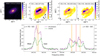 |
Fig. 1 Continuum and CN datasets for Elias 2-27. Top row: high-resolution 240 GHz dust continuum emission (left). The subsequent panels (from left to right) show the integrated intensity (zeroth moment) for CN J = 7/2–5/2 (CN-1), and the CN J = 5/2–3/2 hyperfine group transitions at ~340.035 GHz (CN-2 hf1) and ~340.031 GHz (CN-2 hf2). The frequency of each group is shown at the top of each panel and the ellipses in the bottom left corners show the beam size. In the left panel the green ellipse indicates the region within 230 au from the center (interior region), assuming a flat geometry. Bottom row: Disk integrated spectrum for the whole emitting region (in purple) and for only the interior region (in green). The orange vertical lines indicate the hyperfine transition frequencies that are blended in each peak. When there are multiple transitions, the solid vertical line indicates the one with the higher relative intensity (values in Table 1). The red vertical line is the separation between the CN-2 hyperfine groups. |
Molecular line data, values from CDMS catalog (Müller et al. 2001).
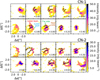 |
Fig. 2 Selection of channel maps for CN-1 (top) and CN-2 (bottom) emission. The number in the top right corner of each panel shows the channel velocity (systemic velocity is 1.95 km s−1), and the ellipse in the bottom left corner the beam size. For the channels used to derive the vertical profile, black dots trace the peak intensity locations along the upper layer of emission. Upper and lower layers of emission, as well as far and near sides of the emission are identified for reference in the bottom panels of the CN-1 emission. A complete panel of the channel map emission is presented in Appendix A for each transition. |
3 Vertical structure analysis
3.1 Height of CN emission
A selection of the channel maps showing the emission from each CN transition is displayed in Fig. 2. We note that for CN-2 the top row shows emission from hf1 and the bottom row from hf2 transitions. For the complete map with all available channels, see Figs. A.1 and A.2 for CN-1 and CN-2, respectively. The systemic velocity of the system is determined to be VLSR ~1.95 km s−1 (Paneque-Carreño et al. 2021). From the channel maps, we identify that the emission does not come from the midplane, but rather originates from a constrained and flared vertical layer. This can be deduced from the separation between the emission from the lower and upper layers, which were visually identified (see Fig. 2) and indicate the vertical location of the gas emission with respect to the disk midplane, as observed from our line of sight. These layers can be visually identified from the channel maps aided by the prior information on the CO distribution (Paneque-Carreño et al. 2021) and the geometry of the system (Huang et al. 2018b). To extract the radial vertical profile we applied the method developed by Pinte et al. (2018), which directly traces the emitting surface from the channel maps. This was done by following the maxima of emission along the upper layer in channels where it is possible to identify the far and near sides of the upper layer (for a detailed sketch see Figs. 2 and 3 of Pinte et al. 2018). This method was used for the extraction of the C18O and 13CO vertical emitting layer in Elias 2-27 (Paneque-Carreño et al. 2021) and in various works, for other sources and/or CO isotopologs (e.g., Law et al. 2021a; Rich et al. 2021; Leemker et al. 2022).
The channels used for this analysis are those between (and including) 1.0–1.4 km s−1 and 2.8–3.2 km s−1 in CN-1, 1.0–1.2 km s−1 and 2.6–3.2 km s−1 for CN-2 hf1, and 4.2–4.6 km s−1 and 6.0–6.4 km s−1 for CN-2 hf2. The selection of channels was done through visual inspection, choosing those where it was possible to identify the upper layer on the near and far sides. Each selected channel was rotated to correct for the disk position angle and to work in Cartesian coordinates for the extraction of the emission maxima (for details, refer to Fig. 2 in Pinte et al. 2018). From the rotated channel emission, we masked the near and far sides of the upper layer. The pixel of peak intensity is automatically identified from the pixels within the mask, sampling every quarter of the beam along the disk major axis. Fig. 2 shows the retrieved peak intensity values (black dots) of the upper layer in some of the selected channels. The height of the emission at a given radial distance is retrieved by applying geometrical relations to the Cartesian location of the emission maxima (for details refer to Pinte et al. 2018).
It has been shown for the CO isotopologs that the emission from the east side of the disk appears to be coming from a layer closer to the midplane than the west side of the disk (Paneque-Carreno et al. 2021). Considering this, we divided the data analysis for CN between east and west sides of the disk, as defined by the projected minor axis. Figure 3 shows the extracted vertical profiles of each CN transition. The data are fitted using an exponentially tapered power law defined as
![Mathematical equation: $z\left( r \right) = {z_0} \times {\left( {{r \over {100{\rm{au}}}}} \right)^\phi } \times \exp \left[ {{{\left( {{{ - r} \over {{r_{{\rm{taper}}}}}}} \right)}^\psi }} \right],$](/articles/aa/full_html/2022/10/aa42693-21/aa42693-21-eq1.png) (1)
(1)
where r is the radial distance from the star along the midplane. The best-fit parameters of the final model are obtained from the median value of the posteriors using a Markov chain Monte Carlo (MCMC) simulation (Goodman & Weare 2010) as implemented by emcee (Foreman-Mackey et al. 2013). The best-fit values of each parameter and its uncertainties (16th and 84th percentile uncertainties derived from the posteriors) are shown in Table 2.
Figure 4 shows the extracted data points separated by disk sides and hyperfine structure. It is apparent that the data from the west side of the disk are consistent between the various transitions, and the best-fit vertical profiles of CN-1 and CN-2 trace the same region, within their uncertainties. The vertical structure from the east side of the disk shows a large scatter in the extracted data, which makes the results vary largely between the CN-1 and CN-2 emission. The scatter may be caused by environmental conditions as the signatures of absorption and ongoing infall from the CO emission are all on the east side of the disk (Paneque-Carreño et al. 2021). Considering the well-defined surface of the west side in all CN transitions and the lack of a strong east–west asymmetry, for the remainder of this work the best-fit vertical profile from the west is used as representative of the CN distribution in the whole disk.
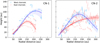 |
Fig. 3 Vertical location of emission from CN-1 (left) and CN-2 (right) transitions, using data obtained from the channel map analysis of the emission. The dataset is separated between the east (red dots) and west (blue dots) sides of the disk, as defined by the semi-minor axis. The solid blue and red curves trace the best-fit exponentially tapered model of each side. The colored regions show the uncertainty of the model, obtained from the spread of the posterior values from our MCMC analysis. |
Best-fit model parameters of exponentially tapered vertical profiles from channel analysis.
3.2 CN versus CO emission
The vertical distribution of the emission from different molecular layers in Elias 2-27 allows us to characterize the various chemical processes occurring in the disk and to estimate the 2D temperature structure of the system (e.g., Pinte et al. 2018; Law et al. 2021b). We compare the CN tracers with previous CO isotopolog observations (Paneque-Carreno et al. 2021) and additionally present the results from extracting the vertical structure of the high-resolution 12CO J = 2–1 DSHARP data (Andrews et al. 2018). We do this comparison only on the west side, due to the cloud contamination that heavily affects the east side in all CO tracers, particularly 12CO J = 2–1 (Pérez et al. 2016; Huang et al. 2018b).
Figure 5 presents the comparison of the derived vertical structures of each molecule for the west side of the disk. As expected from disk chemical models (Bergin et al. 2007; Dutrey et al. 2014), the molecule that traces closest to the midplane is C18O, followed by 13CO for most of the radial extent. The emitting surfaces of the 12CO and CN transitions seem to be tracing almost the same layer up to ~ 120 au. The right panel of Fig. 5 shows the z/r measurements of each tracer. The mean values in each case are 0.53, 0.33, and 0.26 for 12CO, 13CO, and C18O, respectively. For the CN tracers the mean values across the radial extent for both tracers is 0.45. In the discussion (Sect. 6), we analyze and compare this value to what has been derived for other Class II sources. Overall, our results are consistent with CN emission tracing the uppermost layers of the disk, which in Elias 2-27 seem to be significantly vertically extended.
We note that the radial extent of the derived vertical profiles is always smaller than the radial extent of the emission of each tracer. This can be seen from the selected CN channels, shown in Fig. 2, where the black dots tracing the upper layer do not reach the border of the channel emission. In particular for 13CO and C18O, the radial extent of the emission, as traced in the integrated intensity map, is ~650 and ~500 au, respectively (Paneque-Carreno et al. 2021). Therefore, the CO isotopolog emission is roughly two times more extended radially than the farthest radial distance up to where we are able to trace the vertical structure. This occurs because we trace the upper layer of emission directly from the channel maps and only up to radial distances where we can separate the upper and lower layers. At the border of the disk this is not possible. In the case of12 CO, which has the smallest radial extent, we are not able to trace farther out due to the coarse spectral resolution and cloud absorption, which does not allow us to separate the emitting layers beyond ~ 140 au. As we are not able to sample farther radial distances in the 12CO emission, the location of the “turnover” in the height profile is not measured, contrary to the other molecules, and it is unclear if at larger radii 12CO and CN would continue tracing similar locations.
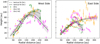 |
Fig. 4 Same data as shown in Fig. 3, but the panels are separated by the west and east sides of the disk. The colored data show the identified CN hyperfine transitions. The solid and dashed black curves show the best-fit vertical models for CN-1 and CN-2, respectively. The light gray region identifies the uncertainties in the best-fit vertical profile, obtained from the spread of the posterior values of the MCMC model. |
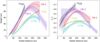 |
Fig. 5 Height (left panel) and z/r (right panel) profiles for the available CO isotopologs and CN transitions in Elias 2-27. The CN emission is separated by a hyperfine group. Solid lines show the best-fit exponentially tapered vertical profile and the shadowed regions show the uncertainty on the best-fit model, derived from the spread of the posteriors in each tracer. Due to the absorption and asymmetries that affect Elias 2-27, the data corresponds to measurements only from the west side of the disk (for all tracers). |
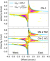 |
Fig. 6 Position-velocity diagrams along the semi-major axis of the disk (PA = 118.8°) for CN-1 (top) and CN-2 (bottom, with two hyperfine group transitions). The offset is positive toward the east side of the disk and negative toward the west. The horizontal lines give the systemic velocity (~1.95 km s−1), shifted for CN-2 hf2 emission to ~5.3 km s−1. The blue curve shows the expected Keplerian velocity curve assuming a flat disk geometry. The dashed black line is the expected Keplerian velocity considering the derived best-fit model for the vertical profile of each tracer. Both models consider a stellar mass of 0.46 M⊙, as derived in Veronesi et al. (2021). The east and west sides of the disk are indicated in the bottom panel for reference. |
3.3 Lack of envelope or large-scale emission
Considering the high z/r values and vertical extension that we derive in Elias 2-27, we analyze the CN emission using a position-velocity (PV) diagram to see if there is any indication of non-Keplerian velocities that may be associated with winds or other effects in the high disk atmosphere (Arce & Sargent 2006). Figure 6 shows the PV diagram along the major axis of the disk, for each of the CN transitions. Overlayed is the expected velocity profile, considering also the best-fit model for the vertical profile and a stellar mass of 0.46 M⊙, as derived by Veronesi et al. (2021). There is no indication of non-Keplerian motion, and we have already discarded any large-scale emission from the emission maps (Sect. 2), as seen in CO isotopologs (Paneque-Carreno et al. 2021); therefore, the disk has intrinsically vertically extended CN emission. It is still plausible that winds or larger-scale structures are present in Elias 2-27, but, due to its high critical densities, CN may not be emissive enough to be detected.
4 Asymmetric distribution of CN emission
The most striking feature from the PV diagram analysis is the extent of the emission to the west side (negative offset), which is larger than on the east side (positive offset). This was discussed in Sect. 2 and relates to the extension difference seen between the north and south regions of the disk, which is not perfectly symmetric in its azimuthal extent with respect to the disk major axis. In the south the radially extended emission stretches azimuthally more toward the west than the east.
To study the north-south radial extent asymmetry, the emission of each tracer is adequately deprojected using the corresponding vertical structure previously derived (Figs. 3 and 4). Azimuthally averaged intensity profiles and stacked spectra are obtained directly from the integrated intensity maps using the get_2D_profile function from gofish (Teague 2019) and sampling in radial bins of 0.1″ (one-third of our beam). The data analysis is separated between the north and south sides of the disk as defined by the major axis. Figure 7 presents the integrated intensity maps and respective intensity profiles for each CN transition. We note that the analysis of CN-2 considers both hyperfine transitions.
The intensity profiles from the north side of the disk show lower values than the south side in both transitions, at all radii. For CN-1 the 98% flux radius of the north side emission is 202.8 ± 11.6 au and for CN-2 179.6 ± 11.6 au (errors correspond to the radial bin size). Figure 7 shows the respective radial contour of the 98% flux radius overlayed on the integrated intensity map of each tracer. We do not resolve any structure from the north side intensity profiles, but beyond 300 au there is a small bump in emission in both transitions. This bump is likely due to the “tail” of the emission that extends slightly toward the north on the southeast side of the disk, and can be seen in the integrated intensity maps (Fig. 7).
Theoretical (Cazzoletti et al. 2018) and observational (Teague & Loomis 2020; van Terwisga et al. 2019; Bergner et al. 2021) studies have shown that the radial profile of CN is expected to present a ring-like feature, which may become shallower or more peaked depending on the disk’s physical properties (Cazzoletti et al. 2018). The integrated intensity maps show a band-like emission in the south, and we identify local maxima and minima from the south profile that we relate to the presence of at least one gap and one ring in each transition. The location of these structures are determined through scrutiny of the radial intensity profile and, when overlayed in the integrated emission maps, there is excellent agreement between the identified locations and the observed band-like structures (top row Fig. 7). For CN-1 the gap is located at 260 au and the ring at 315 au. In CN-2 we determine a position of 230 au for the gap and 275 au for the ring. The small differences in the location of gaps and rings between the two transitions are likely due to the differences in the vertical profiles that are used for deprojecting the emission. We note that in the inner 200 au there may also be tentative gaps and/or rings; however, we are not able to visually assess them in the integrated emission maps with high confidence and do not classify them. The south profile also shows a possible dip in emission in the inner disk, which is expected for CN and is due to the high temperatures near the star that causes CN to be destroyed through its reaction with H2 (Visser et al. 2018).
Figure 8 displays the expected emission surfaces for the upper and lower layers from the best-fit exponentially tapered height profile, assuming they are symmetric. The maximum radial extent in the two surfaces is 400 au which is comparable to the sampled radii in the intensity profiles (Fig. 7). Figure 8 shows that the extended emission in the southernmost part of the disk is not explained by a projection effect of the lower layer, as it is expected to extend only slightly beyond the upper layer. A lack of emission in the north is also observed.
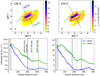 |
Fig. 7 Azimuthal and radial analysis of the CN emission. Top row: integrated intensity of each CN transition. The minor and major axis are marked considering the exponentially tapered vertical profile of the disk. The black elliptical contour marks the north quadrant's 98% flux radius, derived from the intensity profile analysis. The north and south regions are shown in the colors that are used for the intensity radial profiles. The dashed and continuous green contours, respectively indicate the location of the gap and ring detected in the south side emission. Bottom row: intensity profiles derived from the integrated intensity map of each transition. The blue curve traces the north side emission and the green curve the south side emission. The vertical black lines show the location of the north emission 98% flux radius. The vertical green lines show the location of the identified gap (dashed) and ring (solid) in the south side emission. The gray vertical shaded area indicates a one-beam distance from the center. The colored shaded regions show the uncertainty of the intensity profile within each radial bin, obtained as the standard deviation of the data over the number of beams within the radial bin. |
5 Physical properties
To measure the system properties and abundance parameters, we can compute rotational diagrams (Goldsmith & Langer 1999). We used this approach for the CO isotopologs and CN hyperfine group transitions. The analysis of a rotational diagram relates the transition's theoretical properties, particularly the upper state energy, to the measured quantities obtained from the flux of the emission. If several transitions of the same tracer with varied upper state energies are available, this method allows an estimate of both the excitation (or rotation) temperature and the column density of the tracer. As only one transition of each molecule in CO and CN-1, together with the two CN-2 hyperfine group transitions that are too close in their upper energy values (see Table 1) are available, we are not able to simultaneously fit for the temperature and the total column density of each tracer, as was done in previous works (e.g., Goldsmith & Langer 1999; Loomis et al. 2018; Facchini et al. 2021). Therefore, we fit only the total column density and use an estimate for the rotational temperature, as is done by Facchini et al. (2021).
For optically thick tracers, such as 12CO and 13CO, the brightness temperature is coincident with the kinetic temperature. This approach was used in previous works to determine the 2D radial and vertical temperature structure of disks (Pinte et al. 2018; Law et al. 2021b; Izquierdo et al. 2022). We constrained that CN comes from a vertical layer, close to 12CO and higher than 13CO (Fig. 5), so we use the peak brightness temperature profiles of these two CO isotopologs as upper and lower limits for the kinetic temperature in the region from where CN emits. C18O traces a layer just below 13CO, so the 13CO brightness temperature profile can be used as an estimate of the kinetic temperature of the region where C18O emits. We used the online tool RADEX (van der Tak et al. 2007) to estimate the minimum H2 number density needed for the rotation temperature to equal the derived kinetic temperature. For 12CO, 13CO and C18O densities on the order of 105 cm−3 are sufficient. In the case of CN, the number density must be at least 108 cm−3. Models predict that at the location of CN emission the number density is 106–108 cm−3 (Cazzoletti et al. 2018). RADEX simulations show that these lower H2 densities result in lower CN rotation temperatures of 20–40 K assuming a kinetic temperature of ~40 K. These values are within the range that is sampled assuming the 12CO and 13CO temperature profiles as upper and lower limits (see Fig. 9).
The brightness temperature profiles are computed from peak brightness temperature maps and are shown in Fig. 9. Due to the asymmetries and cloud absorption, only the west side emission is considered for CO isotopologs and only the south side emission is considered for CN transitions. 12CO traces between 35 and 60 K, 13CO has a peak temperature of ~28 K, and C18O varies with a mean temperature value of 11.9 K. The CN tracers have mean values of 9.4 K for CN-1 and ~7.1 K for CN-2. All mean brightness temperature values are calculated considering radial distances beyond 40 au to avoid effects of beam smearing in the innermost radii. We note that these profiles do not necessarily correspond to the kinetic and/or rotation temperature at the location of the molecules; this is only true for optically thick tracers. Indeed, 12CO and 13CO show high brightness temperatures above the freeze-out temperature for CO (~21 K, van Zadelhoff et al. 2001; Bisschop et al. 2006). The low brightness temperatures of C18O and both CN transitions are likely caused by the low optical depth of both molecules, which is why these values are not accurate representations of their kinetic temperature. The RADEX simulations of CN result in similar brightness temperatures (10.5 K and 7.8 K for CN-1 and CN-2, respectively) compared to our measurements when the column density of CN is ~6 × 1013 cm−2 and the kinetic temperature 40 K. We note that if the number density is very low in the upper disk layers, CN may be subthermally excited (van Zadelhoff et al. 2003), which would also result in low brightness temperatures.
With the temperature profiles of 12CO and 13CO as estimates of the kinetic temperature in the region where the molecules under study are located, we can obtain an estimate of the total column density and also calculate the optical depth profiles of each tracer. To do this we must first calculate the column density from the upper state (Nu) of each transition using the integrated intensity profiles (obtained in Fig. 7) and the parameters of each transition (see Table 1). For optically thin emission (τ ≪ 1):
 (2)
(2)
Here SvΔv corresponds to the integrated flux density, Ω is the area over which the flux was integrated, and SvΔv is obtained from the integrated intensity profiles of Fig. 7, where the profile has been derived from radial bins. The intensity value from the radial profile must be multiplied by the area of the radial annuli used in each bin and divided by the beam area to obtain the correct flux density units. Each radial annulus has an area Ω. The other parameters are the Einstein emission coefficient of the transition Aul, the speed of light c, and the Planck constant h. If the optical depth (τ) of the emission is non-negligible, then a correction factor Cτ must be applied to the upper state column density,
 (3)
(3)
The column density of the upper state can then be related to the total column density (NT), considering the correction factor, through
 (4)
(4)
where gu is the upper state degeneracy, Eu is the upper state energy, and k is the Boltzmann constant. The value of the partition function Q(Trot) is estimated at each temperature by interpolating with a cubic spline from the values of the CDMS catalog (Müller et al. 2001), as is done in Facchini et al. (2021). Finally, the optical depth of the emission may also be estimated from the upper state column density measurement following
 (5)
(5)
Here Δv is the line width, which is calculated assuming that the broadening from turbulence is negligible and where the thermal broadening is calculated from the temperature and the molecular weight of the molecule under study, and v is the line central frequency. All the other parameters have been defined previously. Equation 5 allows us to express Cτ in terms of Nu, and therefore to solve equation 4 for NT, considering the optical depth properties of the molecules.
Figure 10 shows the results for the total column density NT (top row) and optical depth (bottom row) profiles in 13CO, C18O, and CN tracers. The temperature profile used for the CO isotopologs is only the 13CO profile and the calculation considers the temperature profile uncertainties for the fit. For CN we considered a temperature range, where the upper limit is given by the 12CO temperature profile and the lower limit by the 13CO temperature profile. As the 12CO temperature is only constrained up to ~ 130 au, we consider the last temperature value, 38 K, as a constant value for the remainder of the radial extent. The assumption of constant temperature in the outer radii is based on the temperature profiles of 13CO and C18O that display roughly constant temperature profiles from ~ 100 au outward (see Fig. 9). For the calculation of the CN physical parameters, we do not consider the CO temperature profile errors as they are within the sampled range of temperatures.
Both CN tracers have column densities of 1014 cm−2 in the inner disk that then drop to 1013 cm−2 in the south side outer disk and even lower in the north. On the north side the column density has a steep decline, reaching values bellow 1013 cm−2 beyond 150 au. Likewise, the optical depth of the north side emission rapidly goes to values below unity in the inner 100 au, indicating that the emission is optically thin. The south side of the disk displays a slowly radially decreasing column density which is always within the same order of magnitude, 1013 cm−2. We note that CN-2 displays a localized decrease in the column density of the south side at ~230 au, which coincides with the location of the tentative gap reported in Sect. 4. Regarding the optical depth values of the south side, they are close to unity and show a localized increase at ~ 100 au. Therefore, beyond ~ 150 au CN is optically thin in the whole disk; however, the emission may be marginally optically thick on the south side, particularly inward of ~ 100 au.
For the CO isotopolog emission, our results trace a total column density of ~1015 cm−2 for 13CO and C18O; however, 13CO has a factor of 2-3 higher values. Studies have shown that CO column densities vary between systems depending on the stellar parameters, disk size, and mass (Miotello et al. 2016). Within an order of magnitude, our derived values are in agreement with previous observational and theoretical results (Miotello et al. 2016, 2018; Facchini et al. 2021). The optical depth values of 13CO are above unity, corroborating our initial assumption that it is optically thick. C18O shows marginally optically thin emission from ~ 100 au outward.
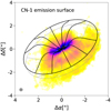 |
Fig. 8 Integrated intensity of CN-1. Overlayed are the emission surfaces using the exponentially tapered vertical profile and assuming symmetry between the upper (black) and lower (gray) layers. |
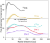 |
Fig. 9 Azimuthally averaged peak brightness temperature profiles of each tracer available for Elias 2-27. The data are extracted only from the west side of the disk to avoid the high absorption effects of the east. In the case of CN the data are only from the south side, due to the additional north-south emission asymmetry. The shadowed colored regions show the uncertainty in the azimuthal averaging of the peak brightness temperature maps, obtained by dividing the standard deviation by the number of independent beams in each radial bin area. |
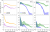 |
Fig. 10 Azimuthally averaged emission properties for CO isotopologs and CN. Top row: column density profiles for each analyzed tracer. Shown together in the leftmost panel are 13CO and C18O. Middle and right panels: column density profile of each CN hyperfine group, separated between north and south sides of the disk. Bottom row: Optical depth profile for each molecule, following the same order as the top row. The horizontal black lines indicate the optical depth of τ = 1. In all panels, the shaded regions show the uncertainty on the model. |
6 Discussion
6.1 Origin of CN emission and comparison to theoretical models
The main formation mechanism of CN is thought to be the reaction of N with vibrationally excited H2 pumped by UV radiation, making CN a tracer of the upper layers of a disk. (Cazzoletti et al. 2018; Visser et al. 2018). Our analysis of CN transitions in Elias 2-27 spatially locates the molecule in a constrained uppermost layer of the disk, with z/r ~ 0.45 in all tracers. The disk is sufficiently flared that we can identify the upper and lower layers of emission in the channel maps (see Fig. 2), and from there directly trace the vertical surface of emission. To our knowledge this is the first time that a direct measurement has been made for CN emission in a disk of moderate inclination, where it is also possible to analyze the radial and azimuthal distribution of material. Previous works have relied on temperature estimates (e.g., Teague & Loomis 2020) or have been conducted in edge-on systems, lacking information on the azimuthal distribution (Ruíz-Rodríguez et al. 2021).
A key feature predicted by models and detected in previous observations of CN is a shallow ring-like structure in the intensity and column density profiles of the disk that is not related to any gas or dust surface density features, but due to chemistry (Cazzoletti et al. 2018; van Terwisga et al. 2019; Teague & Loomis 2020; Ruíz-Rodríguez et al. 2021; Bergner et al. 2021). Both of the analyzed CN transitions show a ring of emission in the south side intensity profiles at 315 au and 275 au. Additionally, the optical depth profiles show a feature at ~ 100 au, where tentative bumps in the radial intensity profile may also be identified (see Fig. 7). All of these features are detected on the south side of the disk. From the north emission we do not retrieve any features, even in the inner (<200 au) region where there is strong CN emission.
Emission of CN is predicted to be optically thin, with typical column densities of ~1014 cm−2, and to be spatially constrained to a thin layer in the upper disk by physical-chemical models (Cazzoletti et al. 2018; Visser et al. 2018). Our results confirm these predictions in most of the radial extension; however, in the inner ~ 100 au some emission may be marginally optically thick (τ = 1–2, see Fig. 10). This could be due to Elias 2-27 hosting a massive gravitationally unstable disk. In agreement with T Tauri models (Cazzoletti et al. 2018), the column density of CN in Elias 2-27 declines less than an order of magnitude on the south side of the disk for both transition groups. The rapid decline in column density on the north side is discussed in Sect. 6.3, and we do not associate it with a chemical process, rather to an effect of the disk environment. Overall, our results of morphology and chemical and physical conditions are in agreement with theoretical predictions for CN emission originating from UV radiation.
Elias 2-27 is likely a gravitationally unstable disk (Paneque-Carreño et al. 2021), and studies focusing on the chemistry of GI disks suggest that CN may be a good tracer of GI spirals (Evans et al. 2015). CN emission originating from the spirals should be observed at the midplane because it would be produced by the desorption of CN from the dust grains along the spirals. CN emits from tens of au above the midplane; therefore, we are not able to compare the dust continuum structure with the CN emission because they are not spatially co-located and there is no signature of any emission from the midplane. This does not rule out self-gravity or that there is no desorption in the midplane. It is possible that, if CN emission originating from GI is present, it is invisible due to the bright emission arising from the higher disk layers or lack of sensitivity in the outer disk. Another option is that, as the spirals are traced between 50 and 200 au (Pérez et al. 2016; Huang et al. 2018b; Paneque-Carreño et al. 2021) and CN is marginally optically thick in this region, it is not possible to observe emission down to the midplane.
6.2 Comparison with resolved emission in other systems
Cyanide has been detected in several Class II systems, both in spatially unresolved (see surveys by, Reboussin et al. 2015; Guilloteau et al. 2013, 2016) and resolved emission (e.g., van Terwisga et al. 2019; Teague & Loomis 2020; Ruíz-Rodríguez et al. 2021; Bergner et al. 2021). There have been various indirect and direct methods employed to measure the vertical location and physical conditions of CN. Overall, there seems to be agreement on the CN conditions in Class II systems. Studies on TW Hya (Kastner et al. 2014; Teague & Loomis 2020) and the Flying Saucer (Ruíz-Rodríguez et al. 2021) both characterize CN column densities between 1013 and 1014 cm–2. In the MAPS dataset (Öberg et al. 2021) the CN column densities peak at 1015 cm–2 for most disks (IM Lup, GM Aur, AS 209, HD 163296, MWC 480); however, the azimuthally averaged column densities are ~1013 cm–2 for most of the radial extent (Bergner et al. 2021). These column density values are in agreement with what we derive in Elias 2-27 (see Sect. 5). MAPS also finds marginally optically thick CN emission in the inner disk (Bergner et al. 2021), in agreement with our results.
Even though the column density and optical depth values are in agreement with previous works and theoretical predictions, the distribution of the CN emission in Elias 2-27 is peculiar. In particular, the vertical extent is much higher than the estimated values for all other Class II sources. Indirect estimates using temperature profiles (TW Hya, Teague & Loomis 2020) or UV-radiation models (MAPS collaboration, Bergner et al. 2021) trace the emitting surface of CN at z/r ~0.2. The CN region in the Flying Saucer disk (Ruíz-Rodríguez et al. 2021), which is the only one to have been modeled directly, shows vertically symmetric CN emission arising from an intermediate molecular layer, lower than 12CO. Ruíz-Rodríguez et al. (2021) also measure very low kinetic temperatures in the CN region (≤ 15 K), which they attribute to the low mass of the star (0.57 M⊙) and extended CN emission, proposing deep X-ray radiation as the origin of the CN. It is interesting to note that Elias 2-27 has a comparable stellar mass of 0.46 M⊙ (Veronesi et al. 2021) to the Flying Saucer, but a very different vertical structure.
In the case of Elias 2-27 CN arises from a high layer of z/r ~ 0.45, indicating that this disk is more vertically extended than previously studied Class II systems. The vertical distribution of CN in Elias 2-27 is similar to that of the Class I source IRAS 04302+2247, where the CN vertical extent traces z/r ~ 0.4 (see Fig. 2 and discussion within Podio et al. 2020). Unfortunately, CN observations in IRAS 04302+2247 are contaminated due to the continuum oversubtraction and absorption, and therefore we do not have further information to compare with our results.
Comparison of the CO vertical structure in Elias 2-27 with other Class II disks shows that the mean z/r values for Elias 2-27 are much higher than those found in the MAPS sample, for all CO isotopologs (Law et al. 2021b). The differences in the 13CO and C18O values may be due to the higher transition (J = 3–2) used in this work; however, for 12CO the same transition as in MAPS is used (J = 2–1). A tentative relation between z/r and the CO radial extent has been proposed such that higher z/r values relate to more extended disks (Law et al. 2021b, 2022). Elias 2-27 has an extended CO disk, consistent with this trend, although this relation also finds that vertically extended CO disks (z/r > 0.3) have mean 12CO brightness temperatures <30 K (Law et al. 2022). As shown in Sect. 5, the brightness temperature of 12CO varies in the range 35–60 K. A larger sample of objects with varied disk and stellar properties is needed to determine if Elias 2-27 is indeed an outlier or if there are more systems with hot and vertically extended gas emission.
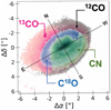 |
Fig. 11 Integrated intensity maps for the tracers studied in this work: 13CO J = 2–1, 13CO J = 3–2, C18O J = 3–2, and CN J = 7/2–5/2 (CN-1). |
6.3 Asymmetric CN, further evidence for infall or a warp?
The CN emission of Elias 2-27 shows an extreme asymmetry between the flux and density profiles on the north and south sides of the disk. This was not seen in previous observations of CO emission (Paneque-Carreno et al. 2021); however, it is similar to the morphology of available NACO L′-band observations (see Fig. 12 in Launhardt et al. 2020). Figure 11 displays the integrated intensity maps for the studied CO isotopologs and CN-1 emission for a comparison of the different radial and azimuthal locations. The east side of the disk shows radially extended CO emission and lack of 12CO, particularly in the northeast quadrant. We propose two scenarios to explain the CN asymmetric emission that are also compatible with the various CO brightness and vertical extent asymmetries.
A decrease in CN production can be linked to the presence of small grains on the north side disk atmosphere, which would shield the surface layers from FUV radiation and reduce the CN emission. An enhanced presence of small grains can be explained by a high dust-to-gas ratio in this region (Nomura et al. 2021) or by the infall of small grains. Infall is the mechanism proposed to be ongoing in Elias 2-27, due to the large-scale emission and variations between the east and west sides observed in 13CO and C18O (Paneque-Carreno et al. 2021). If material is still accreting onto the system, it would explain the vertical differences between east and west and also the north-south extension asymmetry seen in CN.
A second hypothesis to explain the asymmetry is the presence of a warp in the dust disk that creates a shadow and affects the FUV and X-ray radiation received by the north side of the disk (Young et al. 2021). A warped structure is thought to be responsible for the vertical asymmetries detected in the CO emission and the strong kinematical residuals (Paneque-Carreno et al. 2021; Young et al. 2022; Rowther et al. 2022). CN is expected to be a good tracer of the presence of a warp, through asymmetric distribution of its emission (Young et al. 2021). If there is a warped inner disk then we can characterize its inclination direction based on the south-north CN asymmetry, and estimate that it will be aligned with the disk major axis. The presence of a warp will not necessarily affect the CO abundance, although it is expected to affect the CO temperature. Previous studies have shown that the south side of the disk shows brighter CO emission (Pérez et al. 2016; Paneque-Carreno et al. 2021), which would be in agreement with the shadowing of the north side by an inner warp (Young et al. 2021). With our current data we are unable to distinguish between the two proposed scenarios (infall or warp).
Asymmetric CN emission, as reported in this work, has not been observed in any of the resolved Class II observations (van Terwisga et al. 2019; Teague & Loomis 2020; Ruíz-Rodríguez et al. 2021; Bergner et al. 2021); however, there is a similar case in the Class I protobinary source, Oph-IRS 67 (Artur de la Villarmois et al. 2019). Oph-IRS 67 has CN emission traced only toward the south of the disk. This emission likely originates from a photon-dominated region (PDR) beyond the circumbinary disk (Artur de la Villarmois et al. 2019). In addition to CN, the asymmetry in Oph-IRS 67 is also traced in c-C3H2, DCN, and H2CO. It is possible that external radiation could also affect the emission of Elias 2-27. However, we do not have any evidence of PDR regions beyond the disk that could affect the emission. Obtaining observations of PDR sensitive tracers could be useful to further study the asymmetry.
7 Conclusions
We presented an extensive analysis of CN v = 0, N = 3–2, J = 7/2–5/2, and J = 5/2–3/2 emission in Elias 2-27. We also made use of previously published CO isotopolog observations to characterize the vertical stratification and physical properties of the disk (temperature, column density, and optical depth). Through this study Elias 2-27 becomes one of the few Class II systems with a detailed study of the vertical structure and chemical properties of its protoplanetary disk. Our main conclusions are the following:
CN originates at a high vertical location from the disk mid-plane. It traces a region similar to 12CO, at least up to a radial distance of ~ 150 au. CN emits from a vertically constrained and mostly optically thin slab. This is in agreement with theoretical predictions that its main formation mechanism is the reaction of N with UV excited H2.
We trace a strong CN emission asymmetry between the north and south sides of the disk. The extent of CN on the south side goes beyond 400 au, while the 98% flux radius of the north side is 180–200 au. A ringed structure at 230–275 au is observed in the south emission, as predicted by chemical models and similar to observations of CN in other systems. No structure is observed on the north side of the disk emission.
The observed CN asymmetry may be explained by either ongoing infall or a warped inner disk. With the current data and models we are not able to confirm or reject either scenario.
Elias 2-27 is a peculiar Class II source and the studied asymmetries share a strong resemblance with some Class I objects. It has vertically extended (z/r > 0.3) CN and CO isotopolog emission, with high 12CO brightness temperatures and asymmetric CN distribution.
Highly inclined sources such as Elias 2-27 are excellent systems to directly trace and analyze the disk structure and properties. Using optically thick tracers, such as 12CO and13 CO, we can determine the kinetic temperature structure. Combining the temperature profiles with information on the spatial location of various molecules we can recover the physical conditions of the gas.
In summary, this study shows the vertical layering and structure of molecules in Elias 2-27. This is an excellent test case for the importance of simultaneous analysis of multiple tracers to obtain constraints on temperature, column density, and optical depth variations. The favorable inclination and high S/N make it possible to study the 3D disk structure so the emission can be traced radially, azimuthally, and vertically. Future observations with additional tracers, for example HCN, which is UV and temperature sensitive, or c-C3H2 and DCN, which can trace PDR regions, will allow us to fully study the vertical distribution and better understand the origin of the asymmetries in Elias 2-27.
Acknowledgements
This paper makes use of the following ALMA data: #2013.1.00498.S, #2016.1.00606.S and #2017.1.00069.S. ALMA is a partnership of ESO (representing its member states), NSF (USA), and NINS (Japan), together with NRC (Canada), NSC and ASIAA (Taiwan), and KASI (Republic of Korea), in cooperation with the Republic of Chile. The Joint ALMA Observatory is operated by ESO, AUI/NRAO, and NAOJ. Astrochemistry in Leiden is supported by the Netherlands Research School for Astronomy (NOVA), and by funding from the European Research Council (ERC) under the European Union’s Horizon 2020 research and innovation programme (grant agreement No. 101019751 MOLDISK). L.P. gratefully acknowledges support by the ANID BASAL projects ACE210002 and FB210003, and by ANID, – Millennium Science Initiative Program – NCN19_171. This project has received funding from the European Union’s Horizon 2020 research and innovation program under the Marie Sklodowska-Curie grant agreement No 823823, (RISE DUSTBUSTERS).
Appendix A Channel maps
In this section, we present the complete channel maps for each of the CN transitions. Figure A.1 shows the CN-1 emission, which has only one hyperfine group transition. Figure A.2 shows the emission of the two hyperfine group structures of CN-2, imaged with respect to the frequency of CN-2 hf1, 340.0354080 GHz (Müller et al. 2001). The systemic velocity of Elias 2-27 is estimated to be 1.95 km s−1 (Paneque-Carreno et al. 2021).
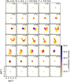 |
Fig. A.1 Complete channel map emission for CN J = 7/2–5/2. In each panel the channel velocity is given in the upper right corner and the beam size of the emission is shown by a black ellipse in the bottom left corner. |
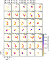 |
Fig. A.2 Complete channel map emission for CN J = 5/2–3/2. In each panel the channel velocity is given in the upper right corner and the beam size of the emission is shown by a black ellipse in the bottom left corner. This transition shows two consecutive hyperfine group transitions. |
Appendix B CO isotopolog observations
Figure B.1 shows the integrated intensity maps and spectra for the CO isotopologs used in this study. The detailed analysis of these data are presented in Andrews et al. (2018) and Huang et al. (2018b) for 12CO and in Paneque-Carreno et al. (2021) for 13CO and C18O. The heavy contamination and absorption in the northeast is visually identified in all tracers, least affecting C18O.
We obtain the integrated fluxes and uncertainties of each tracer (shown in Table 1) from the spectra in the emitting and line-free regions. For the total integrated flux we use an elliptical mask that encircles all of the emission, determined using a curve of growth method on the integrated intensity maps. This mask also determines the region from where the plotted spectra is derived (in Figures 1 and B.1). The uncertainties are derived from the standard deviation of the integrated flux retrieved from 20 line-free regions.
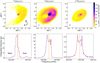 |
Fig. B.1 CO isotopolog emission data used in this study. The top row shows the zeroth moment maps for each CO isotopolog. The beam size is shown in the bottom left corner of each panel. The bottom row displays the spectrum of each tracer. 12CO has a resolution of 0.35 km s−1, while 13CO and C18O have a resolution of 0.111 km s−1. The orange vertical line gives the rest frequency in each case. |
References
- Aikawa, Y., van Zadelhoff, G. J., van Dishoeck, E. F., & Herbst, E. 2002, A&A, 386, 622 [NASA ADS] [CrossRef] [EDP Sciences] [Google Scholar]
- Anderson, D. E., Blake, G. A., Bergin, E. A., et al. 2019, ApJ, 881, 127 [Google Scholar]
- Andrews, S. M. 2020, ARA&A, 58, 483 [Google Scholar]
- Andrews, S. M., Wilner, D. J., Hughes, A. M., Qi, C., & Dullemond, C. P. 2009, ApJ, 700, 1502 [CrossRef] [Google Scholar]
- Andrews, S. M., Huang, J., Pérez, L. M., et al. 2018, ApJ, 869, L41 [NASA ADS] [CrossRef] [Google Scholar]
- Ansdell, M., Williams, J. P., Trapman, L., et al. 2018, ApJ, 859, 21 [NASA ADS] [CrossRef] [Google Scholar]
- Arce, H. G., & Sargent, A. I. 2006, ApJ, 646, 1070 [NASA ADS] [CrossRef] [Google Scholar]
- Artur de la Villarmois, E., Kristensen, L. E., & Jørgensen, J. K. 2019, A&A, 627, A37 [EDP Sciences] [Google Scholar]
- Barenfeld, S. A., Carpenter, J. M., Ricci, L., & Isella, A. 2016, ApJ, 827, 142 [Google Scholar]
- Bergin, E. A., Aikawa, Y., Blake, G. A., & van Dishoeck, E. F. 2007, in Protostars and Planets V, eds. B. Reipurth, D. Jewitt, & K. Keil, 751 [Google Scholar]
- Bergner, J. B., Guzmán, V. G., Öberg, K. I., Loomis, R. A., & Pegues, J. 2018, ApJ, 857, 69 [Google Scholar]
- Bergner, J. B., Öberg, K. I., Bergin, E. A., et al. 2019, ApJ, 876, 25 [Google Scholar]
- Bergner, J. B., Öberg, K. I., Guzmán, V. V., et al. 2021, ApJS, 257, 11 [NASA ADS] [CrossRef] [Google Scholar]
- Bisschop, S. E., Fraser, H. J., Öberg, K. I., van Dishoeck, E. F., & Schlemmer, S. 2006, A&A, 449, 1297 [NASA ADS] [CrossRef] [EDP Sciences] [Google Scholar]
- Cazzoletti, P., van Dishoeck, E. F., Visser, R., Facchini, S., & Bruderer, S. 2018, A&A, 609, A93 [NASA ADS] [CrossRef] [EDP Sciences] [Google Scholar]
- Dutrey, A., Semenov, D., Chapillon, E., et al. 2014, in Protostars and Planets VI, eds. H. Beuther, R. S. Klessen, C. P. Dullemond, & T. Henning, 317 [Google Scholar]
- Evans, M. G., Ilee, J. D., Boley, A. C., et al. 2015, MNRAS, 453, 1147 [NASA ADS] [CrossRef] [Google Scholar]
- Facchini, S., Teague, R., Bae, J., et al. 2021, AJ, 162, 99 [NASA ADS] [CrossRef] [Google Scholar]
- Foreman-Mackey, D., Hogg, D. W., Lang, D., & Goodman, J. 2013, PASP, 125, 306 [Google Scholar]
- Gaia Collaboration (Brown, A. G. A., et al.) 2018, A&A, 616, A1 [NASA ADS] [CrossRef] [EDP Sciences] [Google Scholar]
- Garufi, A., Podio, L., Codella, C., et al. 2021, A&A, 645, A145 [EDP Sciences] [Google Scholar]
- Goldsmith, P. F., & Langer, W. D. 1999, ApJ, 517, 209 [Google Scholar]
- Goodman, J., & Weare, J. 2010, Commun. Appl. Math. Comput. Sci., 5, 65 [Google Scholar]
- Guilloteau, S., Di Folco, E., Dutrey, A., et al. 2013, A&A, 549, A92 [NASA ADS] [CrossRef] [EDP Sciences] [Google Scholar]
- Guilloteau, S., Reboussin, L., Dutrey, A., et al. 2016, A&A, 592, A124 [NASA ADS] [CrossRef] [EDP Sciences] [Google Scholar]
- Guzmán, V. V., Bergner, J. B., Law, C. J., et al. 2021, ApJS, 257, 6 [CrossRef] [Google Scholar]
- Heays, A. N., Bosman, A. D., & van Dishoeck, E. F. 2017, A&A, 602, A105 [NASA ADS] [CrossRef] [EDP Sciences] [Google Scholar]
- Henning, T., & Semenov, D. 2013, Chem. Rev., 113, 9016 [Google Scholar]
- Hily-Blant, P., Magalhaes, V., Kastner, J., et al. 2017, A&A, 603, A6 [Google Scholar]
- Huang, J., Andrews, S. M., Dullemond, C. P., et al. 2018a, ApJ, 869, L42 [NASA ADS] [CrossRef] [Google Scholar]
- Huang, J., Andrews, S. M., Pérez, L. M., et al. 2018b, ApJ, 869, L43 [Google Scholar]
- Ilee, J. D., Boley, A. C., Caselli, P., et al. 2011, MNRAS, 417, 2950 [NASA ADS] [CrossRef] [Google Scholar]
- Ilee, J. D., Walsh, C., Booth, A. S., et al. 2021, ApJS, 257, 9 [NASA ADS] [CrossRef] [Google Scholar]
- Izquierdo, A. F., Facchini, S., Rosotti, G. P., van Dishoeck, E. F., & Testi, L. 2022, ApJ, 928, 2 [NASA ADS] [CrossRef] [Google Scholar]
- Kastner, J. H., Zuckerman, B., Hily-Blant, P., & Forveille, T. 2008, A&A, 492, 469 [NASA ADS] [CrossRef] [EDP Sciences] [Google Scholar]
- Kastner, J. H., Hily-Blant, P., Rodriguez, D. R., Punzi, K., & Forveille, T. 2014, ApJ, 793, 55 [Google Scholar]
- Kastner, J. H., Qi, C., Dickson-Vandervelde, D. A., et al. 2018, ApJ, 863, 106 [Google Scholar]
- Launhardt, R., Henning, T., Quirrenbach, A., et al. 2020, A&A, 635, A162 [NASA ADS] [CrossRef] [EDP Sciences] [Google Scholar]
- Law, C. J., Loomis, R. A., Teague, R., et al. 2021a, ApJS, 257, 3 [NASA ADS] [CrossRef] [Google Scholar]
- Law, C. J., Teague, R., Loomis, R. A., et al. 2021b, ApJS, 257, 4 [NASA ADS] [CrossRef] [Google Scholar]
- Law, C. J., Crystian, S., Teague, R., et al. 2022, ApJ, 932, 114 [NASA ADS] [CrossRef] [Google Scholar]
- Le Gal, R., Öberg, K. I., Loomis, R. A., Pegues, J., & Bergner, J. B. 2019, ApJ, 876, 72 [Google Scholar]
- Leemker, M., Booth, A. S., van Dishoeck, E. F., et al. 2022, A&A, 663, A23 [NASA ADS] [CrossRef] [EDP Sciences] [Google Scholar]
- Long, F., Herczeg, G. J., Pascucci, I., et al. 2017, ApJ, 844, 99 [Google Scholar]
- Loomis, R. A., Cleeves, L. I., Öberg, K. I., et al. 2018, ApJ, 859, 131 [Google Scholar]
- Miotello, A., van Dishoeck, E. F., Kama, M., & Bruderer, S. 2016, A&A, 594, A85 [NASA ADS] [CrossRef] [EDP Sciences] [Google Scholar]
- Miotello, A., van Dishoeck, E. F., Williams, J. P., et al. 2017, A&A, 599, A113 [NASA ADS] [CrossRef] [EDP Sciences] [Google Scholar]
- Miotello, A., Facchini, S., van Dishoeck, E. F., & Bruderer, S. 2018, A&A, 619, A113 [NASA ADS] [CrossRef] [EDP Sciences] [Google Scholar]
- Miotello, A., Facchini, S., van Dishoeck, E. F., et al. 2019, A&A, 631, A69 [NASA ADS] [CrossRef] [EDP Sciences] [Google Scholar]
- Müller, H. S. P., Thorwirth, S., Roth, D. A., & Winnewisser, G. 2001, A&A, 370, L49 [Google Scholar]
- Nomura, H., Tsukagoshi, T., Kawabe, R., et al. 2021, ApJ, 914, 113 [NASA ADS] [CrossRef] [Google Scholar]
- Öberg, K. I., & Bergin, E. A. 2021, Phys. Rep., 893, 1 [Google Scholar]
- Öberg, K. I., Guzmán, V. V., Walsh, C., et al. 2021, ApJS, 257, 1 [CrossRef] [Google Scholar]
- Paneque-Carreño, T., Pérez, L. M., Benisty, M., et al. 2021, ApJ, 914, 88 [CrossRef] [Google Scholar]
- Pérez, L. M., Carpenter, J. M., Andrews, S. M., et al. 2016, Science, 353, 1519 [Google Scholar]
- Piétu, V., Guilloteau, S., Di Folco, E., Dutrey, A., & Boehler, Y. 2014, A&A, 564, A95 [NASA ADS] [CrossRef] [EDP Sciences] [Google Scholar]
- Pinte, C., Ménard, F., Duchêne, G., et al. 2018, A&A, 609, A47 [NASA ADS] [CrossRef] [EDP Sciences] [Google Scholar]
- Pinte, C., Price, D. J., Ménard, F., et al. 2020, ApJ, 890, L9 [CrossRef] [Google Scholar]
- Podio, L., Garufi, A., Codella, C., et al. 2020, A&A, 642, L7 [NASA ADS] [CrossRef] [EDP Sciences] [Google Scholar]
- Reboussin, L., Guilloteau, S., Simon, M., et al. 2015, A&A, 578, A31 [NASA ADS] [CrossRef] [EDP Sciences] [Google Scholar]
- Rich, E. A., Teague, R., Monnier, J. D., et al. 2021, ApJ, 913, 138 [NASA ADS] [CrossRef] [Google Scholar]
- Rowther, S., Nealon, R., & Meru, F. 2022, ApJ, 925, 163 [NASA ADS] [CrossRef] [Google Scholar]
- Ruíz-Rodríguez, D., Kastner, J., Hily-Blant, P., & Forveille, T. 2021, A&A, 646, A59 [NASA ADS] [CrossRef] [EDP Sciences] [Google Scholar]
- Teague, R. 2019, J. Open Source Softw., 4, 1632 [NASA ADS] [CrossRef] [Google Scholar]
- Teague, R., & Loomis, R. 2020, ApJ, 899, 157 [Google Scholar]
- Teague, R., Guilloteau, S., Semenov, D., et al. 2016, A&A, 592, A49 [CrossRef] [EDP Sciences] [Google Scholar]
- van der Marel, N., van Dishoeck, E. F., Bruderer, S., Pérez, L., & Isella, A. 2015, A&A, 579, A106 [NASA ADS] [CrossRef] [EDP Sciences] [Google Scholar]
- van der Marel, N., van Dishoeck, E. F., Bruderer, S., et al. 2016, A&A, 585, A58 [NASA ADS] [CrossRef] [EDP Sciences] [Google Scholar]
- van der Tak, F. F. S., Black, J. H., Schöier, F. L., Jansen, D. J., & van Dishoeck, E. F. 2007, A&A, 468, 627 [NASA ADS] [CrossRef] [EDP Sciences] [Google Scholar]
- van Terwisga, S. E., van Dishoeck, E. F., Cazzoletti, P., et al. 2019, A&A, 623, A150 [NASA ADS] [CrossRef] [EDP Sciences] [Google Scholar]
- van Zadelhoff, G. J., van Dishoeck, E. F., Thi, W. F., & Blake, G. A. 2001, A&A, 377, 566 [NASA ADS] [CrossRef] [EDP Sciences] [Google Scholar]
- van Zadelhoff, G. J., Aikawa, Y., Hogerheijde, M. R., & van Dishoeck, E. F. 2003, A&A, 397, 789 [CrossRef] [EDP Sciences] [Google Scholar]
- Veronesi, B., Paneque-Carreño, T., Lodato, G., et al. 2021, ApJ, 914, L27 [NASA ADS] [CrossRef] [Google Scholar]
- Visser, R., Bruderer, S., Cazzoletti, P., et al. 2018, A&A, 615, A75 [NASA ADS] [CrossRef] [EDP Sciences] [Google Scholar]
- Young, A. K., Alexander, R., Walsh, C., et al. 2021, MNRAS, 505, 4821 [NASA ADS] [CrossRef] [Google Scholar]
- Young, A. K., Alexander, R., Rosotti, G., & Pinte, C. 2022, MNRAS, 513, 487 [NASA ADS] [CrossRef] [Google Scholar]
All Tables
Best-fit model parameters of exponentially tapered vertical profiles from channel analysis.
All Figures
|
Fig. 1 Continuum and CN datasets for Elias 2-27. Top row: high-resolution 240 GHz dust continuum emission (left). The subsequent panels (from left to right) show the integrated intensity (zeroth moment) for CN J = 7/2–5/2 (CN-1), and the CN J = 5/2–3/2 hyperfine group transitions at ~340.035 GHz (CN-2 hf1) and ~340.031 GHz (CN-2 hf2). The frequency of each group is shown at the top of each panel and the ellipses in the bottom left corners show the beam size. In the left panel the green ellipse indicates the region within 230 au from the center (interior region), assuming a flat geometry. Bottom row: Disk integrated spectrum for the whole emitting region (in purple) and for only the interior region (in green). The orange vertical lines indicate the hyperfine transition frequencies that are blended in each peak. When there are multiple transitions, the solid vertical line indicates the one with the higher relative intensity (values in Table 1). The red vertical line is the separation between the CN-2 hyperfine groups. |
| In the text | |
|
Fig. 2 Selection of channel maps for CN-1 (top) and CN-2 (bottom) emission. The number in the top right corner of each panel shows the channel velocity (systemic velocity is 1.95 km s−1), and the ellipse in the bottom left corner the beam size. For the channels used to derive the vertical profile, black dots trace the peak intensity locations along the upper layer of emission. Upper and lower layers of emission, as well as far and near sides of the emission are identified for reference in the bottom panels of the CN-1 emission. A complete panel of the channel map emission is presented in Appendix A for each transition. |
| In the text | |
|
Fig. 3 Vertical location of emission from CN-1 (left) and CN-2 (right) transitions, using data obtained from the channel map analysis of the emission. The dataset is separated between the east (red dots) and west (blue dots) sides of the disk, as defined by the semi-minor axis. The solid blue and red curves trace the best-fit exponentially tapered model of each side. The colored regions show the uncertainty of the model, obtained from the spread of the posterior values from our MCMC analysis. |
| In the text | |
|
Fig. 4 Same data as shown in Fig. 3, but the panels are separated by the west and east sides of the disk. The colored data show the identified CN hyperfine transitions. The solid and dashed black curves show the best-fit vertical models for CN-1 and CN-2, respectively. The light gray region identifies the uncertainties in the best-fit vertical profile, obtained from the spread of the posterior values of the MCMC model. |
| In the text | |
|
Fig. 5 Height (left panel) and z/r (right panel) profiles for the available CO isotopologs and CN transitions in Elias 2-27. The CN emission is separated by a hyperfine group. Solid lines show the best-fit exponentially tapered vertical profile and the shadowed regions show the uncertainty on the best-fit model, derived from the spread of the posteriors in each tracer. Due to the absorption and asymmetries that affect Elias 2-27, the data corresponds to measurements only from the west side of the disk (for all tracers). |
| In the text | |
|
Fig. 6 Position-velocity diagrams along the semi-major axis of the disk (PA = 118.8°) for CN-1 (top) and CN-2 (bottom, with two hyperfine group transitions). The offset is positive toward the east side of the disk and negative toward the west. The horizontal lines give the systemic velocity (~1.95 km s−1), shifted for CN-2 hf2 emission to ~5.3 km s−1. The blue curve shows the expected Keplerian velocity curve assuming a flat disk geometry. The dashed black line is the expected Keplerian velocity considering the derived best-fit model for the vertical profile of each tracer. Both models consider a stellar mass of 0.46 M⊙, as derived in Veronesi et al. (2021). The east and west sides of the disk are indicated in the bottom panel for reference. |
| In the text | |
|
Fig. 7 Azimuthal and radial analysis of the CN emission. Top row: integrated intensity of each CN transition. The minor and major axis are marked considering the exponentially tapered vertical profile of the disk. The black elliptical contour marks the north quadrant's 98% flux radius, derived from the intensity profile analysis. The north and south regions are shown in the colors that are used for the intensity radial profiles. The dashed and continuous green contours, respectively indicate the location of the gap and ring detected in the south side emission. Bottom row: intensity profiles derived from the integrated intensity map of each transition. The blue curve traces the north side emission and the green curve the south side emission. The vertical black lines show the location of the north emission 98% flux radius. The vertical green lines show the location of the identified gap (dashed) and ring (solid) in the south side emission. The gray vertical shaded area indicates a one-beam distance from the center. The colored shaded regions show the uncertainty of the intensity profile within each radial bin, obtained as the standard deviation of the data over the number of beams within the radial bin. |
| In the text | |
|
Fig. 8 Integrated intensity of CN-1. Overlayed are the emission surfaces using the exponentially tapered vertical profile and assuming symmetry between the upper (black) and lower (gray) layers. |
| In the text | |
|
Fig. 9 Azimuthally averaged peak brightness temperature profiles of each tracer available for Elias 2-27. The data are extracted only from the west side of the disk to avoid the high absorption effects of the east. In the case of CN the data are only from the south side, due to the additional north-south emission asymmetry. The shadowed colored regions show the uncertainty in the azimuthal averaging of the peak brightness temperature maps, obtained by dividing the standard deviation by the number of independent beams in each radial bin area. |
| In the text | |
|
Fig. 10 Azimuthally averaged emission properties for CO isotopologs and CN. Top row: column density profiles for each analyzed tracer. Shown together in the leftmost panel are 13CO and C18O. Middle and right panels: column density profile of each CN hyperfine group, separated between north and south sides of the disk. Bottom row: Optical depth profile for each molecule, following the same order as the top row. The horizontal black lines indicate the optical depth of τ = 1. In all panels, the shaded regions show the uncertainty on the model. |
| In the text | |
|
Fig. 11 Integrated intensity maps for the tracers studied in this work: 13CO J = 2–1, 13CO J = 3–2, C18O J = 3–2, and CN J = 7/2–5/2 (CN-1). |
| In the text | |
|
Fig. A.1 Complete channel map emission for CN J = 7/2–5/2. In each panel the channel velocity is given in the upper right corner and the beam size of the emission is shown by a black ellipse in the bottom left corner. |
| In the text | |
|
Fig. A.2 Complete channel map emission for CN J = 5/2–3/2. In each panel the channel velocity is given in the upper right corner and the beam size of the emission is shown by a black ellipse in the bottom left corner. This transition shows two consecutive hyperfine group transitions. |
| In the text | |
|
Fig. B.1 CO isotopolog emission data used in this study. The top row shows the zeroth moment maps for each CO isotopolog. The beam size is shown in the bottom left corner of each panel. The bottom row displays the spectrum of each tracer. 12CO has a resolution of 0.35 km s−1, while 13CO and C18O have a resolution of 0.111 km s−1. The orange vertical line gives the rest frequency in each case. |
| In the text | |
Current usage metrics show cumulative count of Article Views (full-text article views including HTML views, PDF and ePub downloads, according to the available data) and Abstracts Views on Vision4Press platform.
Data correspond to usage on the plateform after 2015. The current usage metrics is available 48-96 hours after online publication and is updated daily on week days.
Initial download of the metrics may take a while.