| Issue |
A&A
Volume 663, July 2022
|
|
|---|---|---|
| Article Number | A98 | |
| Number of page(s) | 22 | |
| Section | Interstellar and circumstellar matter | |
| DOI | https://doi.org/10.1051/0004-6361/202141380 | |
| Published online | 19 July 2022 | |
The protoplanetary disk population in the ρ-Ophiuchi region L1688 and the time evolution of Class II YSOs★
1
European Southern Observatory,
Karl-Schwarzschild-Strasse 2,
85748
Garching bei München, Germany
e-mail: This email address is being protected from spambots. You need JavaScript enabled to view it.
2
INAF – Osservatorio Astrofisico di Arcetri,
Largo E. Fermi 5,
50125
Firenze, Italy
3
School of Cosmic Physics, Dublin Institute for Advanced Studies,
31 Fitzwilliam Place,
Dublin 2, Ireland
4
European Southern Observatory, Av. Alonso de Cόrdova 3107,
Casilla
19001,
Santiago, Chile
5
Dipartimento di Fisica, Università degli Studi di Milano,
Via Giovanni Celoria 16,
20133
Milano, Italy
6
Atacama Large Millimeter/Submillimeter Array, Joint ALMA Observatory, Alonso de Cόrdova 3107,
Vitacura 763-0355,
Santiago, Chile
7
CENTRA/SIM, Faculdade de Ciencias de Universidade de Lisboa,
Ed. C8, Campo Grande,
1749-016
Lisboa, Portugal
8
Lunar and Planetary Laboratory, The University of Arizona,
Tucson, AZ
85721
USA
9
Earths in Other Solar Systems Team, NASA Nexus for Exoplanet System Science,
USA
10
Freie Universität Berlin, Institute of Geological Sciences,
Malteserstr. 74-100,
12249
Berlin, Germany
11
SUPA, School of Physics & Astronomy, University of St. Andrews North Haugh,
St Andrews, KY16 9SS,
UK
12
Univ. Grenoble Alpes, CNRS, IPAG,
38000
Grenoble, France
13
Institute for Astronomy, University of Hawaii,
Honolulu,
HI
96822
USA
Received:
25
May
2021
Accepted:
22
December
2021
Abstract
Context. Planets form during the first few Myr of the evolution of the star-disk system, possibly before the end of the embedded phase. The properties of very young disks and their subsequent evolution reflect the presence and properties of their planetary content.
Aims. We present a study of the Class II/F disk population in L1688, the densest and youngest region of star formation in Ophiuchus. We also compare it to other well-known nearby regions of different ages, namely Lupus, Chamaeleon I, Corona Australis, Taurus and Upper Scorpius.
Methods. We selected our L1688 sample using a combination of criteria (available ALMA data, Gaia membership, and optical and near-IR spectroscopy) to determine the stellar and disk properties, specifically stellar mass (M⋆), average population age, mass accretion rate (Ṁacc) and disk dust mass (Ṁdust). We applied the same procedure in a consistent manner to the other regions. Results. In L1688 the relations between Ṁacc and M⋆, Mdust and M⋆, and Ṁacc and Mdust have a roughly linear trend with slopes 1.8–1.9 for the first two relations and ~1 for the third, which is similar to what found in the other regions. When ordered according to the characteristic age of each region, which ranging from ~ 0.5 to ~5 Myr, Ṁacc decreases as t−1, when corrected for the different stellar mass content; Mdust follows roughly the same trend, ranging between 0.5 and 5 Myr, but has an increase of a factor of ~3 at ages of 2–3 Myr. We suggest that this could result from an earlier planet formation, followed by collisional fragmentation that temporarily replenishes the millimeter-size grain population. The dispersion of Ṁacc and Mdust around the best-fitting relation with M⋆, as well as that of Ṁacc versus Mdust are equally large. When adding all the regions together to increase the statistical significance, we find that the dispersions have continuous distributions with a log-normal shape and similar widths (~0.8 dex).
Conclusions. This detailed study of L1688 confirms the general picture of Class II/F disk properties and extends it to a younger age. The amount of dust observed at ~1 Myr is not sufficient to assemble the majority of planetary systems, which suggests an earlier formation process for planetary cores. The dust mass traces to a large extent the disk gas mass evolution, even if the ratio Mdust/Mdisk at the earliest age (0.5–1 Myr) is not known. Two properties are still not understood: the steep dependence of Ṁacc and Mdust on M⋆ and the cause of the large dispersion in the three relations analyzed in this paper, in particular that of the Ṁacc versus Mdust relation.
Key words: protoplanetary disks / submillimeter: planetary systems / stars: formation
Full Tables A.1–G.1 are available at the CDS via anonymous ftp to cdsarc.u-strasbg.fr (130.79.128.5) or via http://cdsarc.u-strasbg.fr/viz-bin/cat/J/A+A/663/A98
© ESO 2022
1 Introduction
The formation of planets in disks around young stars has been actively studied for a long time, especially since the discovery of exoplanets and the realization that most stars in the Galaxy are likely to host planetary systems.
Based on Solar System evidence and the study of the incidence of disks around young stars, it has been inferred that planet formation has to occur in the first few million years since the formation of the host star (e.g., Johansen et al. 2014; Pfalzner et al. 2015, and references therein). It is now widely accepted that planets form in protoplanetary disks, which are formed as the byproduct of the star formation process (e.g., Shu et al. 1987). The lifetimes of protoplanetary disks set an upper limit to the planet formation process of about few Myr, which is consistent with the timescale for the formation of the pristine bodies in the Solar System (e.g., Hernández et al. 2008, and references therein). There is increasing evidence that at least some planets form early in the evolution of the star–disk systems (e.g. Keppler et al. 2018; Pinte et al. 2018, 2019, 2020; Casassus & Pérez 2019; Alves et al. 2020), most likely when the disk is still accreting matter from the collapsing core, based on the lack of solids available to form planetary cores in disks older than 0.5–1 Myr (e.g. Greaves & Rice 2010; Najita & Kenyon 2014; Ansdell et al. 2016; Testi et al. 2016; Manara et al. 2018; Sanchis et al. 2020) In these early evolutionary stages (so-called Class 0 or Class I protostars, Lada 1987; Andre et al. 1993), the properties of the collapsing core, such as the rotation and magnetic field, are likely to affect the disk structure itself, and, as a consequence, the planet population that is undergoing formation. The first high-angular-resolution observations by ALMA of HL Tau, a young stellar object at the transition between Class I and Class II, show structures that may be interpreted as having resulted from advanced planet formation (ALMA Partnership 2015).
At a slightly later stage, when the envelope has almost entirely dispersed (so-called Class II young stellar objects Lada 1987), disks carry the imprints of the planetary systems that they host (e.g., gaps and rings), and the presence of planets affects the disk’s evolution (e.g. Isella et al. 2016). On the other hand, disks lose matter due to accretion onto the central star and winds; the decrease in the gas density over time may affect, in turn, further planet growth and the dynamical evolution of young planetary systems (Hartmann et al. 2016; Ercolano & Pascucci 2017). The solid disk component changes over time as grains grow and drift with respect to the gas toward the star, then becoming trapped in winds and accretion flows. In addition, grains are lost to rocky planets and planetesimals, which, on the other hand, may also collide and fragment, replenishing the grain population (Johansen et al. 2014; Turner et al. 2014). The environment, which hosts gravitational interactions in dense clusters and strong UV radiation field due to nearby massive stars, can also play a role (e.g., Winter et al. 2018, 2020).
One possible way to study the interplay and the timeline of all these processes relies on the availability of measurements of some basic bulk quantities, such as stellar and disk masses, for a large number of objects of different masses and in different star-forming regions. The Class II evolutionary phase lasts much longer than Class I/0, and statistical studies of disk properties were initiated long time ago. Their results include, for example, a measurement of the disk lifetime of few Myr by measuring the fraction of objects with near-IR excess (Hernández et al. 2008) and evidence of accretion (Fedele et al. 2010) as function of the typical age of each region, as well as the dependence of the mass accretion rate on the age of the central star, as predicted by viscous accretion disk models (Hartmann et al. 2016). Other works have provided unexpected results, such as the steep correlation between the mass accretion rate and the stellar mass  found in Taurus (Muzerolle et al. 2005) and ρ-Oph (Natta et al. 2006), which was interpreted as having resulted from a spread in the properties of the parental cores (Dullemond et al. 2006), although alternative explanations have not been excluded (e.g. Ercolano et al. 2014; Vorobyov & Basu 2009; Alexander & Armitage 2006; Clarke & Pringle 2006; Hartmann et al. 2006; Gregory et al. 2006).
It is, however, only in the last decade that with the advent of large surveys both in the optical and mm wavelengths, these kinds of studies have become possible for a large number of star-forming regions and possible evolutionary patterns have been established. In particular, the greatly improved sensitivity provided by VLT’s second-generation instruments and by ALMA have allowed for population studies of accretion and disk properties to be extended down to very-low-mass stars (VLMS) and brown dwarfs (BDs), and, more generally, lower-mass disks, allowing us to effectively undertake broader population studies (Testi et al. 2016; Sanchis et al. 2020). The broad wavelength range and sensitivity of VLT/X-shooter has been used to derive reliable stellar parameters and mass accretion rates (e.g. Alcalá et al. 2017; Manara et al. 2015, 2017, 2020), while complementary ALMA surveys have allowed us to measure millimeter dust continuum and molecular line emission for disks over a large range of stellar masses, from brown dwarfs to solar-mass stars (e.g. Ansdell et al. 2016; Pascucci et al. 2016; Barenfeld et al. 2016; Testi et al. 2016; Cazzoletti et al. 2019). While the original hope to constrain the disks gas masses from the observations of the carbon monoxide isotopologues have turned out to be more uncertain than originally expected (e.g., Miotello et al. 2017; Bergin & Williams 2017), several complementary lines of evidence suggest that the millimeter continuum flux is a good proxy of the solids mass in disk albeit with systematic uncertainties due to the poorly constrained dust physical and chemical properties (Turner et al. 2014; Andrews 2015). Moreover, a number of recent studies have started to investigate the different evolution of the dust millimeter grains and the gas component of the disk by including the effects of growth, drift, and fragmentation (Pinilla et al. 2020; Sellek et al. 2020; van der Marel & Mulders 2021; Michel et al. 2021). On the other hand, the few available attempts to directly measure disk masses from gas kinematical modeling show a remarkable consistency with estimates from the dust continuum measurements (assuming the canonical gas to dust ratio of 100, e.g. Veronesi et al. 2021, Izquierdo et al., in prep.).
Notwithstanding the above uncertainties, several important trends for disk bulk properties have been confirmed: the steep dependence of Ṁacc on M⋆ (e.g. Alcalá et al. 2017; Manara et al. 2017, 2020), and the steeper than linear correlation between Mdust and Macc (e.g. Ansdell et al. 2016; Pascucci et al. 2016; Barenfeld et al. 2016). Manara et al. (2016) showed for the first time that Ṁacc increases almost linearly with the disk (dust) mass, as predicted by viscous evolution models. This was also confirmed by Mulders et al. (2017), who also pointed out that the dispersion of the data points cannot be easily reconciled in the simplified viscous evolutionary models, unless the age of the disks is comparable with the viscous timescale (Lodato et al. 2017). A clear trend showing a decrease in Mdisk(or Mdust) with the age of the region was found when comparing the 2–3 Myr Lupus and Chamaeleon I with the 5–8 Myr Upper Scorpius (Ansdell et al. 2017). Other intriguing results have also been reported. For example, Upper Scorpius has large mass accretion rates and a huge dispersion of values when compared to Lupus and Chamaeleon I for disks of the same mass (Manara et al. 2020), contrary to the expectations of viscous evolutionary models (see e.g. Lodato et al. 2017; Rosotti et al. 2017).
Very recently, the ALMA data of two very young regions, ρ-Oph (Williams et al. 2019; Cieza et al. 2019) and Corona Australis (Cazzoletti et al. 2019) seem to indicate that the disk (dust) mass in these regions is smaller than in the older Lupus and Chamaeleon I regions. This is unexpected, and potentially very interesting, if confirmed. However, the results for ρ-Oph could be contaminated by a significant component of older objects, belonging to groups of different ages, including the overlapping Upper Scorpius population, in the same region (Esplin & Luhman 2020); moreover, only the cumulative mass distribution of the regions were compared, as a characterization of the stellar properties of the objects (M⋆ in particular) was not available.
In this paper we present a new analysis of the young stellar photosphere and disk properties for the Class II/F protoplanetary disks in the ρ-Ophiuchi L1688 region. This sample is then compared with other well known star forming regions in the Solar neighborhood, namely Lupus, Chamaeleon I, Corona Australis, Taurus and Upper Scorpius, with the aim of analyzing potential evolutionary trends. In all cases, we base our analysis on new membership and distance information derived from spec-troscopy and the Gaia DR2 data, and we derive the disk and stellar properties in a homogeneous way.
In Sects. 2 and 3, we describe the ρ-Ophiuchi L1688 sample properties, new observations, and results. In Sect. 4, we describe the properties of the objects in the other star-forming regions analyzed in this paper. The results are discussed in Sect. 5. Conclusions follow in Sect. 6.
2 Ophiuchus L1688 Sample
We focus our study on L1688, the densest and youngest region of star formation in Ophiuchus (Wilking et al. 2008; Esplin & Luhman 2020). We selected young stars with disks classified as Class II or F, observed with ALMA, and with estimates of three crucial photospheric parameters, namely spectral type (SpT), extinction (AK), and J-band magnitude, which allow us to estimate the stellar properties. In the following sections we summarize the details of the selection process.
2.1 ALMA L1688 Data
2.1.1 ALMA 1.3 mm Data from the ODISEA Survey
The Ophiuchus region was the subject of an extensive 1.3 mm ALMA survey of the young stellar population (The Ophiuchus DIsk Survey Employing ALMA (ODISEA), Cieza et al. 2019; Williams et al. 2019, W19 in the following). The survey includes all the protostars identified in the Spitzer “Cores to Disks” Legacy project (Evans II et al. 2009) for a total of 279 objects (Class I, Flat spectrum, Class II and Class III). Of these, 172 are classified as Class II and 50 as Class F1. The surveyed area covers, but extends beyond L1688, including, for example, members of the older Upper Scorpius association and of other young groups in the ρ-Ophiuchi star forming region (e.g. L1689 and L1709, among others). We will discuss in Sect. 2.2 how we selected from the ODISEA survey the members of L1688 that will be used in this study.
2.1.2 ALMA 0.89 mm data for VLMS and BDs
As part of a survey of very low mass stars and brown dwarfs with disks, we observed with ALMA a total of 25 objects at 0.89 mm with ALMA (Testi et al. 2016, T16 from now on, and this work). A detailed discussion of this sample is given in Appendix A.
2.2 Membership and Spectroscopy
Esplin & Luhman (2020, EL20 in the following) have recently published a new, critical analysis of the Ophiuchus region. Their aim was to establish the membership of all known objects with evidence of youth in addition to known spectral type in a region which includes the three main dark clouds of Ophiuchus (L1688, L1689, L1709) and a substantial area north of L1688, encompassing the majority of W19 ALMA region. They separated the Ophiuchus subgroups members from other populations by applying kinematic criteria to the Gaia second data release. The result is a catalog of 373 members, 259 candidate members and 59 stars with kinematics that are inconsistent with membership in Ophiuchus.
We focus on L1688, the youngest core of star formation in the region. It occupies an area on the plane of the sky defined according to Fig. 1 of EL20. In this region, there are 154 young stellar objects classified as Class F or Class II by W19 and Cieza et al. (2019, based on previous Spitzer surveys). Of these, 88 are classified as members of L1688 and 7 as candidate members by EL20. For all these objects we adopted the spectral type, extinction and J-band magnitude as given by EL20.
To these we added three sources (J162435.2-242620, J162618.1-243033, J162732.6-243323) in the L1688 region, for which EL20 does not provide spectral types. However, we did found spectroscopically determined spectral types, extinction, and J-band magnitude values for them in the literature (van der Marel et al. 2016; Mužić et al. 2012; McClure et al. 2010).
Seven of the BDs observed in Band 7 by T16 or in this study are not present in the ODISEA survey (GY92-320 from T16, and GY92-141, CFHTWIR-Oph-58, CFHTWIR-Oph-66, CFHTWIR-Oph-77, CFHTWIR-Oph-90, CFHTWIR-Oph-98, from this paper). They are all classified as member or candidate member by EL20, and we adopt their parameters from EL20, as above.
In summary, the L1688 sample analyzed in this work contains 105 objects.
2.3 Stellar Parameters
Using the J-band magnitude, the extinction and the spectral type, for each source we estimated photospheric luminosity L⋆ and effective temperature Teff. We derived the J-band extinction from AK using the ratio AJ/AK = 2.63 (EL20) and computed for each star the effective temperature Teff according to the SpT-Teff relation used by Testi et al. (1998) and Luhman et al. (2003) (see also the references quoted in these papers, as well as the analysis in Testi 2009). The luminosity is then derived from the J-band magnitude, corrected for extinction, the Gaia distance, and the bolometric correction to the J magnitude as compiled by Testi et al. (1998) and Luhman (1999). For the stars with no Gaia distance we adopt the average value of 139.4 pc (EL20).
We proceeded in the same way for objects with extinction and spectral type from other studies. In each case, we used the extinction law quoted in the relevant paper to convert to a consistent set of J-band extinctions (see Sect. 2.2).
The resulting Hertzsprung-Russel (HR) diagram is shown in Fig. 1 (top left panel), with overlaid the tracks from Baraffe et al. (2015). Uncertainties on both Teff and L⋆ can be very large, especially in a region of high extinction as L1688 (see, e.g., EL20). Manara et al. (2015) quote at least one spectral sub-class and >0.2dex in L⋆, even when using X-shooter spectra with their broad wavelength coverage and high sensitivity. As discussed in the literature (e.g., Alcalá et al. 2017), uncertainties in the spectral classification may be larger for G- and K-types, as compared to M-dwarfs. We thus estimated an error of 1.5–2 sub-classes for the higher-mass objects in our sample.
Stellar masses are derived by comparing the location on the HR diagram to the pre-main sequence evolutionary tracks of Baraffe et al. (2015), when possible; for objects with stellar mass larger than 1.4 M⊙, we used the Siess et al. (2000) tracks. The choice of these evolutionary tracks is meant to facilitate the comparison with previous works on a numberofstar-forming regions (e.g. Alcalá et al. 2017; Sanchis et al. 2020). For a given set of evolutionary tracks, and for the bulk of the stellar masses and ages covered in our sample, the evolutionary tracks are nearly vertical in the HR diagram; hence, the derived values of M⋆ are affected mostly by uncertainties in the spectral type. Values of M⋆ for objects more luminous than the evolutionary tracks was derived by vertically extrapolating the tracks. Typical uncertainties are at least ±10%, but can be significantly larger for individual objects with highly uncertain spectral type.
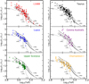 |
Fig. 1 HR diagrams for the six star-forming regions, as labelled in each panel. Stellar evolutionary tracks (dotted lines) and isochrones (solid lines) are from Baraffe et al. (2015); masses and ages are as labelled. |
2.4 Mass Accretion Rate
The largest survey of mass accretion rates in L1688 was published by Natta et al. (2006). Accretion luminosities were computed for a sample of 104 Class II/F stars using the L(Paβ) in 96 cases or L(Brγ) for the remaining 8 luminosity as a proxy for Lacc. Of the 105 objects in our sample, 60 have been observed by Natta et al. (2006). We recomputed the line luminosity for the distance and extinction adopted in this paper and derive Lacc from the relations of Alcalá et al. (2017).
We then derived the mass accretion rates from the relation Ṁacc = 1.25LaccR⋆/(GM⋆), with R⋆. computed from the photospheric luminosities and effective temperatures.
We note that in Natta et al. (2006), who selected their sample from the ISOCAM YSOs in the study of Bontemps et al. (2001), a total of 140 objects were observed, of which 35 were classified as Class III and 105 as Class II. The 45 ISOCAM Class II objects excluded from the sample discussed in this paper are either not present in the ALMA ODISEA survey or are classified as non-members of L1688 by EL2O.
3 Results for L1688
The L1688 sample of 105 objects is the largest among the nearby star forming regions (d < 150–160 pc), spanning a large range of spectral types, stellar luminosities (between ~10−3 and 10 L⊙), and masses (from ~0.01 to ~1 M⊙). The M⋆ distribution is shown in Fig. 2.
3.1 Relationship Between Disk Dust Mass and Stellar Mass
The dust mass in each disk is computed from the millimeter flux, assuming optically thin emission and Rayleigh-Jeans approximation, according to:
 (1)
(1)
where Fmm is the observed flux, d the distance, κv the dust opacity at the frequency of the observations, and Bv the Planck function at the dust temperature Tdust. Adopting κv = 2.3 cm2 g−1 at 1.3 mm and Tdust = 20K, as in Ansdell et al. (2017), Eq. (1) gives Mdust/M⊙ ~ 9 × 10⁻¹¹ d2 F1.3 mm with d in pc and F1.3 mm in mJy. For the 7 L1688 BDs with only 0.89 mm fluxes from ALMA, we assume a ratio of F1.3 mm/F0.89 mm = 0.44 (see Appendix A).
In the following, we define the total (gas + dust) disk mass as Mdisk = 100 × Mdust. Also, we use Mdust or Mdisk depending on the context. We note that, in fact, both are simply proportional to the measured millimeter flux.
The distribution of Mdust as a function of M⋆ is shown in Fig. 3. Compared to the compilation of Testi et al. (2016), this is a significant improvement. With the exception of a handful of BDs, all disk masses come from a coherent set of ALMA measurements at 1.3 mm; the membership and stellar parameters have been derived in a consistent and more accurate way for a sample that is three times greater, covering the range of stellar masses in a more uniform way.
We note that for stars above ~0.4 M⊙, all disks have been detected at 1.3 mm, thanks to the sensitivity of the ODISEA ALMA survey (Cieza et al. 2019). The 2 orders of magnitude in dispersion for Mdust at any given M⋆ is consistent with what is observed in other nearby star forming regions (e.g., Pascucci et al. 2016; Ansdell et al. 2017, Ansdell et al. 2016).
Figure 3 shows lines Mdisk ∝ (M⋆/M⊙) and Mdisk (Μ⋆/Μ⊙)2, for different proportionality coefficients, as labeled. We confirm the results presented by Testi et al. (2016) in their study of the dust masses in disks around BDs, namely that the relation between Mdust and M⋆ when a sufficiently broad range of M⋆ is considered is steeper than linear. This result has since been confirmed by most nearby Class II disk populations studied so far (e.g. Pascucci et al. 2016; Ansdell et al. 2017). To quantify the relationship between Mdust and M⋆, following the approach used in similar studies, we performed a power law fit to the data shown in Fig. 3, using the method developed by Kelly (2007) (see Appendix H for details). When using the full sample, including upper limits, we find that Mdust~M⋆1.5 (cyan thick line in figure), but we note that this result is mostly constrained by the limited data in the BDs regime. A fit for M⋆ ≥0.15 M⊙ gives Mdast~M⋆1.9 (orange thick line in figure), with an uncertainty of ~0.4.
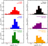 |
Fig. 2 Stellar mass distribution for the six regions, as labelled. The total number of stars in each regions is given in the respective panel. The distribution for L1688 is shown in all the other panels by the red line. |
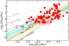 |
Fig. 3 Dust mass, Μdust, as a function of the stellar mass M⋆ for L1688. Filled dots are actual measurements, open dots with arrows are upper limits. Cyan lines plot the results of a linear fit over the whole range of Μ⋆; orange lines the results when stars with M⋆ < 0.15 M⊙ are excluded (see text). For comparison, we plot the relations Μdisk ∝ Μ⋆2 (dashed black lines) and Μdisk ∝ M⋆(dotted grey lines) for different values of the Μdisk/Μ⋆ ratio, as labelled. Note that, as always, Μdisk = 100 × Mdust. |
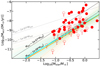 |
Fig. 4 Mass accretion rate as a function of M⋆ for L1688; symbols as in Fig. 3. Cyan lines show the results of a linear fit over the whole range of M⋆; orange lines the results when stars with M⋆ < 0.15 M⊙ are excluded (see text). For comparison, we plot the relations Ṁacc ∝ Μ⋆2 (dashed black lines) and Ṁaœ ∝ M⋆(dotted grey lines) for different values of the Ṁacc/M⋆ ratio, as labeled. |
3.2 Relationship Between Mass Accretion Rate and Stellar Mass
Figure 4 shows the measured Ṁacc values and upper limits in L1688 as a function of the stellar mass. Grey dotted and black dashed lines show the relations expected for a linear and quadratic dependence of the mass accretion rates on the stellar mass. As already noted in other star-forming regions (e.g. Muzerolle et al. 2005; Natta et al. 2006; Alcalá et al. 2017; Manara et al. 2017), when extending to the very low mass stars and BDs, the Ṁacc values are lower than expected from a linear relation.
To quantify the relationship between Ṁacc and M⋆, following the approach used in similar studies, we performed a power law fit to the data shown in Fig. 4, using the method developed by Kelly (2007) (see Appendix H for details). When using the full sample, including upper limits, we find that Ṁacc~M⋆1.9 (cyan thick line in figure). A fit for M⋆ ≥ 0.15M⊙ gives a similar result, within the uncertainties (Ṁacc ~ M⋆1 8 orange thick line in figure). These values are nearly identical to the results of Natta et al. (2006), who did not have a significant number of spectral type classifications for the Ophiuchus Class II YSOs; hence, their stellar masses were derived from the extinction corrected J-band luminosities assuming a single 1 Myr isochrone. The net result is that photospheric parameters derived in our previous study were more uncertain and that the upper limits were correlated with the stellar luminosity and mass, as they were also derived from the J-band luminosities (see Natta et al. 2006, for details of the procedure).
4 Comparison with Other Star-Forming Regions
The new ALMA data, membership determination, and stellar properties set a much firmer foundation for the characterization of L1688 disk properties, allowing us to add it to the sample of the other nearby star-forming regions to study the evolution of disk populations. For this purpose, we selected a sample of the best-studied nearby regions and re-determined their stellar and disk properties, as described in this section, to ensure an approach that is as homogeneous as possible.
4.1 Data Selection
4.1.1 Lupus
The Lupus disk population has been extensively studied with ALMA by Ansdell et al. (2016, 2018); Sanchis et al. (2020), and the photopheric and disk accretion properties with X-shooter by Alcalá et al. (2014, 2017). Recently, Luhman (2020) re-assessed the membership to the Lupus cloud of all candidates using Gaia data, as in EL2O. We apply the same criteria described in Sect. 2.2 to the selection of objects of Class F/II that are members or candidate members according to Luhman (2020), and have been observed with ALMA. This results in a reduction from the original 95 objects observed by Ansdell et al. (2018) to the 63 studied in this paper. All these objects have a determination of stellar parameters and accretion rates from X-shooter observations (Alcalá et al. 2017), which we recomputed using the new Gaia distances. Disk masses are computed from the data in the 1.3 mm survey of Ansdell et al. (2018), with the same prescription used for L1688.
The table of the adopted properties for the Lupus sources is reported in Appendix C.
4.1.2 Upper Scorpius
A fraction of the Upper Scorpius disk population has been surveyed with ALMA at 0.88 mm by Barenfeld et al. (2016), who also report the photospheric effective temperatures and luminosities for their sample. While it remains incomplete, this is nonetheless the largest homogeneous millimeter survey of Upper Scorpius available to date. Luhman & Esplin (2020) analyzed the membership properties of Upper Scorpius using Gaia data. We applied the same selection criteria as before to define the sample of the 74 Upper Scorpius Class F and II discussed in the following, using, as before, the new Gaia distances to recompute photospheric and accretion properties. Manara et al. (2020) sampled a subset of 34 sources from the Barenfeld et al. (2016) study with X-shooter to derive disk accretion properties – all of these are included in our sample. We note that Manara et al. (2020) has already used the new Gaia distances. Disk masses are computed from the Barenfeld et al. (2016) fluxes converted to 1.3 mm using the average ratio 0.4 (spectral index 2.4) as derived for the disk populations of several nearby star-forming regions (Ansdell et al. 2018; Ribas et al. 2017; Tazzari et al. 2021), and Eq. (1). The table of the adopted properties for the Upper Scorpius sources is reported in Appendix D.
4.1.3 Chamaeleon I
A large fraction of the Chamaeleon I disk population has been surveyed with ALMA at 0.89 mm by Pascucci et al. (2016), while Manara et al. (2017) carried out an extensive spectroscopic campaign to accurately determine stellar photospheric properties and accretion rates. Following Manara et al. (2019), we used Gaia DR2 to correct the derived parameters using the new individual (for the stars in the Gaia catalogue) and average distances. Starting from Pascucci et al. (2016), and applying the same selection criteria as before we derive a sample of 79 Chamaeleon I Class F and II stars, which we use in the following. The Gaia membership of the Cha I region was recently analyzed by Galli et al. (2021), and 64 of our 79 stars are confirmed members, with their distance estimates consistent with our values. Of the remaining 15 stars, 13 do not pass the strict quality standards of Galli et al. (2021), but are classified as members by Esplin et al. (2017); the remaining two stars are considered candidate members according to the criteria of Pascucci et al. (2016) and Manara et al. (2017). As for Upper Scorpius, we computed disk masses from the 0.89 mm fluxes converted to 1.3 mm fluxes with the same constant factor of 0.4 and Eq. (1). The table of the adopted properties for the Chamaeleon I sources is reported in Appendix E.
4.1.4 Corona Australis
The Corona Australis regions was surveyed with ALMA by Cazzoletti et al. (2019), who also reports on the distance estimate and the photospheric parameters of the stars. The Gaia membership of the Corona Australis region was recently analyzed by Galli et al. (2020), and only 15 of our 36 stars are present in the Gaia members catalog, probably because of the strict quality threshold applied on the data and the high extinction in the Corona Australis region. We thus adopted as candidate members all the sources in Cazzoletti et al. (2019). The table of the adopted properties for the Corona Australis sources is reported in Appendix F.
4.1.5 Taurus
The most complete compilation of submillimeter continuum measurements of young stars with disks in the Taurus region is that of Akeson et al. (2019). Recently Esplin & Luhman (2019) revisited the membership and properties of the Taurus young stars using Gaia data. To derive the stellar photospheric parameters we thus followed the same procedure as in the L1688 region (see Sect. 2.2). The table of the adopted properties for the Taurus sources is reported in Appendix G.
4.2 Stellar Mass Distributions and Ages
Figure 1 shows the HR diagram for the six regions, while the mass distribution is shown in Fig. 2. While only L1688 – and to some extent Taurus – extends to very low mass objects and BDs, above M⋆ ~ 0.15 M⊙, all the regions are well sampled.
A comparison of the HR diagrams shows that L1688 is the youngest, with ages similar to those of Taurus and Corona Australis; Lupus and Chamaeleon are likely older by ~ 1–2Myr, while Upper Scorpius is about 5 Myr. This agrees with the relative age distribution in the literature, where there is general consensus that L1688 is one of the youngest region of star formation, several Myr younger than Upper Scorpius (see, e.g., Esplin & Luhman 2020). For each region, Table 1 shows the median values, first and third quartiles of the stellar age distribution of the stars in our samples, derived from comparison to the Baraffe et al. (2015) evolutionary tracks. To avoid the parameter range where the evolutionary tracks are closer to each other than the uncertainties on the stellar temperature and luminosity, we considered only stars with masses in the range of 0.15 ≤ M⋆/M⊙ ≤ 1.0. In the following, we use these as the representative ages for our samples of Class II objects in each region. The uncertainties on age estimates derived by comparing the location of the stars on the HR diagram with evolutionary tracks are well known (see, e.g., D’Antona 2017; Herczeg & Hillenbrand 2015; Braun et al. 2021) and beyond the purpose of this paper.
Characteristic age of the regions.
4.3 Mdust Cumulative Distributions
One methodology that has been widely used in the past to compare the typical disk dust mass in different star-forming regions is the cumulative mass distribution (e.g., Andrews et al. 2013; Ansdell et al. 2016).
Figure 5 shows the dust mass cumulative distribution for each star-forming region computed using the Kaplan-Meier estimator from the lifelines2 package, which takes into account the upper limits using a proper technique for left censored datasets. Lupus, Taurus, and Chameleon have a similar cumulative function for the disk (dust) mass and differ from those of Upper Scorpius and Corona Australis, while the L1688 cumulative dust mass function is placed between these two groups. This confirms the results already shown by W19, namely, of an apparent discrepancy, with the expectation of a monotonic decline of the dust mass content with age, also noted by Cazzoletti et al. (2019).
An important limitation of the comparative analysis of the cumulative mass distributions is that it does not take into account the properties of the sampled stellar masses. We attempt to address this limitation in the following sections.
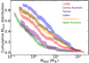 |
Fig. 5 Comparison of the Μdust cumulative distributions in the various regions. The color-shaded regions show the uncertainty range for each distribution. |
4.4 Mdust–M⋆ Relation
The distribution of values of the disk mass versus M⋆ is shown in Fig. 6 for all the regions. As for L1688, we performed for each region, a power-law fit to the data (Kelly 2007) for the whole sample and for M⋆ > 0.15 M⊙ (see Appendix H); the results are shown in Fig. 6 and Table H.1. With the possible exception of Taurus, the inclusion of the lower-mass objects does not change the values of the slopes within the uncertainties. Slopes vary between ~1 for CrA and Taurus (we note, however, that the fits are heavily affected by upper limits), ~1.3 for Chamaeleon and ~2 for L1688, Lupus and Upper Scorpius. There is no clear trend with the age of the regions, as L1688, Lupus and Upper Scorpius have similarly steep slopes. We note that the slopes derived for some of the regions are slightly different from those reported by Pascucci et al. (2016) and Ansdell et al. (2017), due to a combination of the revision of our samples based on the Gaia membership and distance, along with the new photospheric parameters, and the stellar mass range (see also Hendler et al. 2020).
4.5 Ṁacc–M⋆ Relation
Figure 7 plots the mass accretion rate Ṁacc as a function of M⋆ for the four regions where homogeneous estimates of Ṁacc are available. Linear fits for the whole samples and the more massive stellar population M⋆ > 0.15 M⊙ are shown in Appendix H. The results are given in Table H.1 and shown in Fig. 7. All regions have steep slopes (in the range 1.6–2.3) when the whole sample is considered, consistent with each other within the uncertainties. For stellar masses larger than 0.15 M⊙, the nominal values for Lupus and Chamaeleon I slopes are smaller; however, the difference is not significant considering the uncertainties. Alcalá et al. (2017) and Manara et al. (2017) found that a fit with a break and two slopes is a more accurate description of the data for Lupus and Chamaeleon I. We do not see evidence that this is the case in the L1688 region (see also Fiorellino et al. 2021, for the case of NGC 1333). This may point to evolutionary differences in the very-low-mass stars and BDs as compared to stars. In this paper we focus on the evolution of the objects more massive than about 0.15 M⊙, as the samples of objects below ~0.1 M⊙ are still strongly affected by incompleteness and small number statistics.
4.6 Ṁacc–Mdisk Relation and Accretion Disk Lifetimes
Figure 8 shows the relation between Ṁacc and the disk mass Mdisk for all objects with measured Mdisk (upper limits are not included). Linear fits are described in Appendix H. The results show that the trend is about linear for all four regions, with no significant difference between them (see Fig. 8), nor for different M⋆ intervals. A roughly linear trend was found by Manara et al. (2016) in the Lupus star-forming region, by Mulders et al. (2017) in Lupus and Chamaeleon I, and by Manara et al. (2020) in Upper Scorpius. We confirm these results and find that this is also the case for L1688.
The ratio Mdisk/Ṁacc provides an interesting timescale for disk evolution after the first million years, and is plotted in Fig. 9 as a function of M⋆. We can see that there is no trend with M⋆ for M⋆ > 0.15 M⊙; at lower M⋆, there is a hint of larger values of this ratio among Lupus (as noted by Sanchis et al. 2020) and Chamaeleon I objects, but not in L1688. However, there are very few objects at these low masses, and a large number of Ṁacc upper limits in L1688, which, taken all together, limit the significance of this result.
4.7 Dispersion Around the Linear Fits
All regions show a broad range of Mdust and Ṁacc values for the same M⋆. Inspection of Figs. 6, 7, and 8 shows that in all cases the observed values are distributed over an interval of at least two dex, with no obvious trends. We quantify this dispersion by measuring the distance (in dex units,  ) of the values from the best fits at fixed values of M⋆. We consider the sample of M⋆ ≥ 0.15 M⊙ and add together the results of all the regions. In this way, we correct for potential systematic differences among regions and significantly improve the statistical significance of the results, which are shown in Fig. 10 for Mdust (top panel) and Ṁacc (middle panel), respectively.
Both distributions are well described by a Gaussian with a width of σ = 0.65 and 0.87 for Mdust and Ṁacc, respectively, when upper limits are included and treated as measurements. Figure 10 shows also the results when they are excluded (dotted lines); the distributions are still well described by Gaussians with similar widths (σ =0.64 and 0.84, respectively). Upper limits are concentrated among objects below the fitted relations (negative values of  ), but do not change the overall distribution too much.
Finally, we have performed a similar analysis for the dispersion of the observed values of Ṁacc for the same Mdisk (Fig. 10, bottom panel). The distribution is again well represented by a Gaussian, with σ = 0.84 and 0.73 when upper limits are included or not, similarly to that of the other two distributions.
5 Discussion
In this section, we discuss the disk properties defined in the previous sections as a function of the characteristic age of each region. We note that this approach assumes that one region “ages” into another one and that other differences, such as the initial conditions under which disks form or the environment in which they evolve are irrelevant.
5.1 Time Evolution of Dust Mass and Mass Accretion Rates
In order to control how the results may be affected by the strong dependence of both Mdisk and Ṁacc on M⋆, we both use the full 0.15–3 M⋆ interval (removing the dependencies on M⋆ as derived in Appendix H), along with narrow intervals of M⋆, and we compute the median and quartile values for the various disk (sub-)samples. The results are shown as a function of the age of the region in Figs. 11 and 12.
In all cases, we compute how medians and percentiles are affected by upper limits by comparing the two extreme cases: assuming that the true value of the quantity is equal to the estimated upper limit, or that the true value is much smaller than the smallest measured value in the full sample. The two values of the medians are often very similar; when they are not, the range between the two extremes appears as a filled box in the figure. In some case, the number of upper limits is larger than the number of detections in the given M⋆ interval. In such case the lower extreme of the median range cannot be defined by our procedure and we show the median as an arrow. The 75% percentile is always defined.
A close inspection of the results shows that it is possible to identify an overall temporal trend, similar for both Mdust and Ṁacc: a slow, linear decrease with time (∝ t−1), as shown in Fig. 11. This temporal evolution is expected for viscous disks (under the assumption that Mdust traces the total disk mass). Hartmann et al. (2016) report an almost linear time decrease of Ṁacc ∝ t−1.07 in a large sample of individual stars from various star forming regions with masses in the interval 0.3–1.0 M⊙ and ages, derived from the location of the individual stars on the HR diagram, ranging from ~0.1 to ~20 Myr.
As shown in Fig. 9 there is no evidence for a time evolution of the ratio τ = Mdisk/Ṁacc. If we assume a simple viscous evolution of the disk populations, we expect that when the age of the disk population is much larger than the viscous timescale, τ will increase with the age of the region (Lodato et al. 2017). This is, in fact, not the case and τ remains constant at ~ 1 Myr over an interval of ages of several Myr, presenting a challenge for simple viscous evolution models.
 |
Fig. 6 Dust mass Mdust is shown as a function of the stellar mass for the six regions. In each panel the lines show the result of a linear fit performed including the whole range of M⋆ as discussed in the text. The orange line shows the best fit for L1688. |
5.2 Disk Mass and Dust Mass
The similarity of the time evolution of Mdust to that of Ṁacc indicates that Mdust is a good overall, first-order tracer of Mdisk, as already noted by Manara et al. (2016). The disk mass is computed assuming a constant, canonical factor of Mdisk= 100 × Mdust. This is just a normalization factor. In fact, the overall trend, which is similar to that of Ṁacc, does not change as long as Mdisk/Mdust remains roughly constant over the time interval spanned by the regions studied in this paper. If planet formation occurs at an earlier stage and significantly depletes the disk of its grain population, then our assumption of Mdisk/Mdust = 100 in the 1 Myr old Class II population of L1688, Taurus and Corona Australis may grossly underestimate the total disk mass at that age. In this case, the true timescale (Mdisk/Ṁacc) will be proportionally higher than the τ ~ 106 yr indicated in Fig. 9. However, the constancy of τ in the following evolution remains. The results of this paper do not give any direct constraint on the value of Mdisk/Mdust in the youngest Class II samples, but suggest that, whatever the initial value, the gas and dust evolution is not massively decoupled in the following few million years, at least in disks that survive the passing of time.
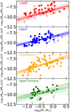 |
Fig. 7 Mass accretion rate as a function of M⋆ for the four regions for which Ṁacc is known, as labeled. In each panel we show the result of a linear fit performed including the whole range of M⋆ as discussed in the text. The orange line shows the best fit for L1688. |
5.3 Dispersions
The three relations we analyzed are dominated by the large dispersion of points around the best-fitting relations (see Fig. 10), well above the observational uncertainties (see e.g. discussion in Manara et al. 2020; Mulders et al. 2017). The distribution of the distances from the best fits is smooth and well described by Gaussian functions. The dispersion is a characteristic of the whole populations and it is not influenced by a limited number of peculiar objects; therefore, it is therefore related to a dispersion of the underlying physical processes. The dispersion in the Ṁacc–Mdisk relation is similar to the one in the other two relations, namely MdiSk versus M⋆ and Ṁacc versus M⋆. A possible interpretation is that stars of the same age and mass can accrete at very different mass accretion rates, even when their disk mass is the same (e.g. Dullemond et al. 2006; Mulders et al. 2017; Manara et al. 2020). The origin of this is still not understood, and there have been a number of different suggestions (initial conditions, time variability, magnetic fields, disk dissipation processes), none of them fully satisfactory. Alternatively, it has been suggested that disks of the same gas mass can have very different dust evolution causing an additional dispersion in the relation between the (dust-derived) disk masses and mass accretion rates (Sellek et al. 2020). Our results (Fig. 10) may provide quantitative constraints to both interpretations.
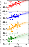 |
Fig. 8 Maœ as a function of the disk mass Μdisk = 100 × Mdust for all the objects with measured Μdisk. In each panel, we show the result of a linear fit performed including the whole range of M⋆, as discussed in the text. The orange line shows the best fit for L1688. |
5.4 Mdust Excess in Lupus and Chamaeleon I
Figure 12 shows an interesting effect, on top of the time dependence defined by the dotted line, namely, displaying how the two regions with ages of ~2 – 3 Myr (Lupus and Chamaeleon I) have, on average, more massive disks than expected for their age. The difference is a factor of ~3 and it is rather uncertain. We note that it appears to be more pronounced for low-mass stars. It is, however, potentially very interesting, as dynamical models of the evolution of dust, planetesimals, and planetary populations in disks predict that the total mass of grains detectable at mm wavelengths may not decrease monotonically with time, but increase after the formation of sufficiently large planets, as these excite a population of planetesimals into eccentric orbits and trigger collisional fragmentation (Turrini et al. 2012, 2019; Gerbig et al. 2019). If this is indeed the case, then our results suggest that the peak of this process should occur at 2–3 Myr, and point to an earlier phase of planet formation. In this view, planets form on timescale of about 0.5–1 Myr, or even less. Objects such as L1688, Taurus, and Corona Australis may be at a stage where planets have already formed, but the creation of a significant population of secondary grains is just beginning. Their dust content is still dominated by the remaining fraction of the original solid population. Over the following 1–2 Myr, collisional fragmentation of planetesimals increases the dust mass; further in time, this dust production stops and the disk dust mass declines.
This view is consistent with the current idea that planet formation has to occur at very early ages, before the age of the youngest populations discussed in this paper. We note that this generation of a secondary population of dust at 2–3 Myr is not large enough to change the overall trend of the time evolution, as discussed in Sect. 5.1.
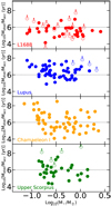 |
Fig. 9 Ratio Μdisk/Ṁacc is plotted as a function of M⋆ for all objects with measured Μdisk. The dotted line corresponds to Μdisk/Ṁacc = 1 Myr. |
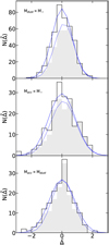 |
Fig. 10 Distribution of the dispersion from the individual best-fitting relations for of all regions combined (see text). The dispersion (in dex units, |

5.5 Disk Dispersal Processes
If, as discussed in Sect. 5.1, Ṁacc and MdiSk decrease with time approximately as t−1, after 5 Myr the disk mass and mass accretion rate would only be reduced by a factor of 5. This would result in very long dispersal times, much longer than the typically observed value of few Myr (Hernández et al. 2008). The fact that Class III objects show mm emission similar to that of field debris disks (Lovell et al. 2021; Michel et al. 2021) suggests that disks may need to dissipate very fast, much faster than the ages of those we observe in the surviving Class II populations. The most likely candidates for these fast dissipation processes are photoevaporation or planet formation. Population synthesis models predict a clear tail of low values in the Ṁacc vs. MdiSk relation, as most of the disk dispersal and disk planet interaction processes predict a faster decline of Ṁacc compared to Mdisk. This is not observed in the present study (see Fig. 10) and it is possible that the short timescale of these processes makes it very difficult to find evidence for this in the properties of the surviving disks (see also Manara et al. 2019). Our large samples, which span a large range of ages, offer, in principle, the possibility of identifying the tail of objects in the dispersal phase, but we do not find any clear evidence for such a tail (see Sect. 4.7). In Fig. 10 (bottom panel), the few objects at  could be further investigated as potentially residing in the phase of dispersal.
We conclude that the analysis of bulk population properties of Class II disks does not tell us how disks disappear; these follow the slow evolution that is consistent with viscosity or wind-driven accretion, not the catastrophic events that lead to the disk dissipation on short timescales. The potential impact of different planetary architectures and dust evolution on the timescales of disk dissipation is currently being discussed and may be a dominant factor in explaining the observed dispersion of properties (see Sect. 5.3, and Sellek et al. 2020; Pinilla et al. 2020; van der Marel & Mulders 2021; Michel et al. 2021).
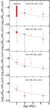 |
Fig. 11 Ṁacc medians and percentiles as a function of age for L1688 (red), Lupus (blue), Chamaeleon I (yellow), and Upper Scorpius (green). From top to bottom: for the full range of stellar masses 0.15 ≤ Μ⋆/Μ⊙ < 3.0 (after removing the trends with M⋆ as derived in Appendix H), and for three mass bins, as labeled. In each case, the dotted line shows the trend Ṁacc ∝ t−1, normalized to the median value for L1688. The filled box shows the possible range of the median value, following the treatment of upper limits described in the text. |
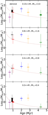 |
Fig. 12 Mdust medians and percentiles as a function of age for L1688 (red), Corona Australis (purple), Taurus (black), Lupus (blue), Chamaeleon I (yellow), and Upper Scorpius (green). From top to bottom: For the full range of stellar masses 0.15 ≤ Μ⋆/Μ⊙ < 3.0 (after removing the trends with M⋆ as derived in Appendix H), and for three mass bins, as labeled. In each case, the dotted line shows the trend Mdust ~ t−1, normalised to the median value for L1688. The filled box shows the possible range of the median value, following the treatment of upper limits described in the text. |
6 Summary and Conclusions
This paper provides a description of disk masses and mass accretion rates in the ρ-Oph region L1688, one of the richer and younger star-forming regions in the Solar neighbourhood. Our selection criteria require that the objects have been observed with ALMA (W19), have distance and membership properties taken from Gaia (EL20), and an estimate of spectral type and extinction. We estimated Teff, L⋆, and M⋆ for each object and derived a characteristic age of the population of ~1 Myr. The relations between Mdisk and M⋆, Ṁacc and M⋆, and Ṁacc and Mdisk are qualitatively similar to those observed in other regions, with a roughly linear trend with slopes ~ 1.8–1.9 for the first two relations and ~ 1 for the third (for M⋆ > 0.15 M⊙). All three relations have large dispersion around the best fit.
The main interest in studying L1688 is to put it in the context of the other regions studied so far, and to characterize, in particular, the disk evolution over time. To this end, we re-analyzed the data for Corona Australis, Taurus, Lupus, Chamaeleon I and Upper Scorpius, using the same selection criteria and analysis as for L1688. The stellar and disk properties are given in the Appendix B. The results confirm the results of previous analyses in the literature, with differences due to different selection criteria and assumptions, that do not affect the global picture.
We note that our selection of Class II/Flat disks limits our results to the evolution from the time the star-disk systems emerge from their parental core to the time they lose the near or mid-IR excess used in disk classification. The star-forming regions in this paper range in age from about 0.5 to 5 Myr. When ordered according to the characteristic age of each region, there is evidence of a relatively slow decline of Ṁacc, roughly as t−1. A similar trend is observed when plotting the properties of a sample of individual stars as function of the stellar age (Hartmann et al. 2016) and is expected if disk evolution is controlled by some kind of viscosity.
The behavior of Mdust over time is more complex. Assuming the same conversion factor from millimeter flux density to dust mass, the values of Mdust in L1688 (age ~1 Myr) and in Upper Scorpius (age ~4.5 Myr) show a decline that is consistent with the same trend as observed in Ṁacc. However, an interesting aspect of the Mdust behavior is that it is not monotonic with age, but shows an increase of a factor of ~3 at the age of 2–3 Myr above the overall time trend. A similar behavior is predicted by some theoretical models where the earlier (<1 Myr) formation of planets excites a population of planetesimals into eccentric orbits, subsequently triggering a collisional fragmentation cascade (Turrini et al. 2012, 2019; Gerbig et al. 2019). This result is very interesting as it is a potential confirmation of early planet formation. Nonetheless, we note that our observations suggest that the amount of millimeter detected dust is only a factor of ~3 larger than the value expected from the evolutionary trend. In turn, this means that the total disk mass estimates, based on a conversion from the millimeter continuum flux, are probably qualitatively correct within the same factor.
All the relations have large dispersions. To minimize the limitations induced by the relatively small samples, for all the regions we combined the dispersions from each of the individual fits. We find that the dispersions of measurements around each of the three relationships Mdust versus M⋆, Ṁacc versus M⋆, and Ṁacc versus Mdisk have continuous distributions with a roughly log-normal shape and similar widths (~±0.8 dex), with no outliers. In particular, in the Ṁacc versus Mdisk relation, there is no evidence of a tail of objects with low Ṁacc. This confirms the need for a rapid disk-dispersal mechanism, such as photoevaporation or planet formation, which, however, do not seem to significantly affect the disk properties considered in this paper during the Class II/F phase.
When compared to the predictions of viscous disk evolution, we confirm an almost linear decrease of both Macc and Mdisk over time. However, viscous models encounter a number of difficulties, already noticed in the literature (e.g. Mulders et al. 2017; Manara et al. 2020), which our study confirms. Among them, there is the large dispersion in the Ṁacc–Mdisk relation, which does not change over time, along with the fact that the ratio of these two quantities is constant in time.
The origin of two properties remains puzzling: the steep dependence of Ṁacc and Mdisk on M⋆ and the cause of the large dispersion in the three relations analyzed in this paper; in particular that of the Ṁacc versus Mdisk relation. These dispersions could be related to a particular combination of different effects, including initial conditions, dust evolution, and disk dispersal properties (e.g. Dullemond et al. 2006; Lodato et al. 2017; Sellek et al. 2020; Somigliana et al. 2020).
An important caveat is that even the relatively large and well-characterized samples discussed in this paper are still limited in a number of ways. Two major limitations are (still) the sensitivity limits and the completeness of the samples. For example, values of Ṁacc in L1688 come from a relatively old work (Natta et al. 2006), while about 50% of the measurements are upper limits and many of the recently classified members by EL20 were not included. Even the extensive ALMA survey has a large number of upper limits and is incomplete. The same is true for Upper Scorpius.
To attain progress in the understanding of disk populations evolution and dissipation, it is necessary to overcome the limitations outlined above. It is equally important to dedicate significant amounts of ALMA time to obtain systematic measurements of molecular gas properties, as well as disk radii. Extending similar studies to the earlier (e.g., Class 0 and I) and later (Class III) phases of disk evolution is necessary to explore the planet formation phase, as well as disk dissipation.
Acknowledgements
This work was partly supported by the Italian Ministero dell Istruzione, Università e Ricerca through the grant Progetti Premiali 2012 – iALMA (CUP C52I13000140001), by the Deutsche Forschungsgemeinschaft (DFG, German Research Foundation) – Ref no. 325594231
FOR 2634/1 TE 1024/1-1, and by the DFG cluster of excellence Origins (www.origins-cluster.de). This project has received funding from the European Union’s Horizon 2020 research and innovation programme under the Marie Sklodowska-Curie grant agreement No 823823 (DUSTBUSTERS) and from the European Research Council (ERC) via the ERC Synergy Grant ECOGAL (grant 855130), and the ERC Advanced Grant The Dawn of Organic Chemistry (grant 741002). K.M. acknowledges funding by the Science and Technology Foundation of Portugal (FCT), grants No. IF/00194/2015, PTDC/FIS-AST/28731/2017, and UIDB/00099/2020. I.dG.-M. is partially supported by MCIU-AEI (Spain) grant AYA2017-84390-C2-R (co-funded by FEDER).
Appendix A ALMA 0.89mm Observations of BDs and Very Low Mass Objects in L1688
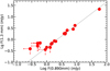 |
Fig. A.1 Observed 1.3mm versus 0.890mm flux for the L1688 objects with measurements at 1.3mm and 0.98 mm. |
Testi et al. (2016, T16) observed 17 BDs and very-low-mass objects in L1688 at 0.89mm. We note that 1 of the 18 published in Τ16 (ISO-Oph 164) was, in fact, an erroneous observation (while the source coordinates in Table 1 in Τ16 are correct, the source really observed with ALMA was GY92-317, located at 16:27:40.10 −24:38:36.46). Nine additional sources were observed as part of the ALMA project ADS/JAO. ALMA 2017.1.01243. S on April Ist, August 17th, and 18th, 2018. A total of 44 Antenna Elements were available during the observing sessions. We used the ALMA Band 7 receivers tuned to a frequency of ~338 GHz, the total effective bandwidth usable for continuum was approximately 6 GHz and the 13CO(3–2) line was covered in one of the spectral windows of the correlator. Standard calibration was performed by the ESO ALMA Regional Centre, and the flux density scale is expected to be accurate within 5%. The total time on source was about 12min per target. Peak, integrated fluxes, and upper limits are computed as described in T16.
The 0.89mm fluxes and upper limits are displayed in Table A.1 for the total sample of 25 objects; data from T16 are marked as such in the last column of the table. All objects but ISO-Oph42 are classified as member or candidate member by EL2O; distances, spectral types, and extinction come from their paper. For ISO-Oph42, stellar parameters are from Mužić et al. (2012), as given in T16, corrected for the new Gaia distance. Stellar luminosity and mass are computed as described in Sect. 2.
W19 gives measurements or upper limits for 19 of the objects in Table A.1. Figure A.1 plots the 1.3mm flux versus the 0.890 flux for all the objects with both measurements; it shows that there is a very tight relation, with a ratio F1.3mm/F0.89mm =0.44. The corresponding spectral index is αmm = 2.2.
We caution that, in order to make a comparison with the recent literature, in this paper we adopt a conversion factor between observed millimeter flux and dust mass using a constant dust temperature of 20 K. This is different from the assumption of Τ16, who used the prescription  (following Andrews et al. 2013). The derived Mdust values are systematically lower than those in T16, by a factor of 3–10; see also the discussion on the adopted value of Tdust in Τ16 Appendix A. However, these different assumptions do not affect the slope of the Mdust-M⋆ relation.
VLMO with ALMA 0.89mm data.
Appendix B ρ-Ophiuchi/L1688 data
Parameters of the Class F and II sources in L1688 studied in this paper are shown in Table B.1. We report in the following order:
88 sources observed by Williams et al. (2019) and classified as members of L1688 by Esplin & Luhman (2020)
7 sources observed by Williams et al. (2019) and classified as candidate members by Esplin & Luhman (2020)
3 sources observed by Williams et al. (2019) in the geographical region of L1688 and with spectral types and magnitudes from McClure et al. (2010); Mužić et al. (2012); van der Marel et al. (2016)
7 VLMS and BDs sources observed either as part of this study or in Testi et al. (2016) and classified as members of L1688 by Esplin & Luhman (2020)
Properties of L1688 objects
Appendix C Lupus Data
Parameters of the Class F and II sources in Lupus studied in this paper are shown in Table C.1.
Properties of Lupus objects
Appendix D Upper Scorpius Data
Parameters of the Class F and II sources in Upper Scorpius studied in this paper are shown in Table D.1.
Properties of Upper Scorpius objects
Appendix E Chamaeleon I Data
Parameters of the Class F and II sources in Chamaeleon I studied in this paper are shown in Table E.1.
Properties of Chamaeleon I objects
Appendix F Corona Australie Data
Parameters of the Class F and II sources in Corona Australis studied in this paper are shown in Table F.1.
Properties of Corona Australis objects
Appendix G Taurus Data
Parameters of the Class F and II sources in Taurus studied in this paper are shown in Table G.1.
Properties of Taurus objects
Appendix H Mdust vs. Μ⋆, and Ṁacc vs. Μ⋆ Regression
In this appendix we show the results of applying the Kelly (2007) method to the samples analyzed in this paper. We used the python implementation of the linmix code3. In all cases we included the non-detections in the dataset, properly accounting for censored data in the computations.
In Figs. H.1 and H.2 we show the results of fitting the following relation:
 (H.1)
(H.1)
to the Corona Australis, Taurus, and L1688 (Fig. H.1, from top to bottom), and Lupus, Chamaeleon I and Upper Scorpius (Fig. H.2, from top to bottom) samples. In all figures the left panel shows the data and the resulting fit including the full population (cyan) and only the subsample with Μ⋆ ≥ 0.15 M⊙ (orange).
In Fig. H.3 we show the results of fitting the following relation:
 (H.2)
(H.2)
to the L1688, Lupus, Chamaeleon I and Upper Scorpius (from top to bottom) samples. In all figures the left panel shows the data and the resulting fit including the full population (cyan) and only the subsample with M⋆ ≥ 0.15 M⊙ (orange).
In Fig. H.4 we show the results of fitting the following relation:
 (H.3)
(H.3)
to the L1688, Lupus, Chamaeleon I and Upper Scorpius (from top to bottom) samples. In all figures the left panel shows the data and the resulting fit including the full population (cyan) and only the subsample with M⋆ ≥ 0.15 M⊙ (orange).
The values derived for all regions and all relationships are reported in Table H.1. The value of δ in the table is a measure of the dispersion of the points from the fit (see linmix documentation).
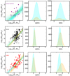 |
Fig. H.1 Power-law fits to the Mdust vs. M⋆ relationships. From top to bottom: Results for Corona Australis, Taurus, and L1688. From left to right: Plot of the dataset and fit results, probability distributions for the a parameter in Eq. H.1, and for the β parameter in Eq. H.1. Cyan is when all objects are included, orange when objects with Μ* < 0.15 M⊙ are excluded. |
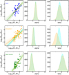 |
Fig. H.2 Power-law fits to the Mdust vs. M⋆ relationships. From top to bottom: Results for Lupus, Chamaeleon I, and Upper Scorpius. From left to right: Plot of the dataset and fit results, probability distributions for the a parameter in Eq. H.1, and for the β parameter in Eq. H.1. Cyan is when all objects are included, orange when objects with Μ⋆ < 0.15 M⊙ are excluded. |
Results of the power-law fits to the Mdust vs. M⋆ relations. The value of δ is a measure of the dispersion from the fit (see linmix documentation).
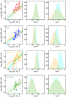 |
Fig. H.3 Power-law fits to the Ṁacc vs. M⋆ relationships. From top to bottom: Results for L1688, Lupus, Chamaeleon I, and Upper Scorpius. From left to right: Plot of the dataset and fit results, probability distributions for the a parameter in Eq. H.2, and for the β parameter in Eq. H.2. |
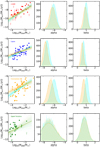 |
Fig. H.4 Power-law fits to the Ṁacc vs. Μdisk relationships. From top to bottom: Results for L1688, Lupus, Chamaeleon I, and Upper Scorpius. From left to right: Plot of the dataset and fit results, probability distributions for the a parameter in Eq. H.3, and for the β parameter in Eq. H.3. |
References
- Akeson, R. L., Jensen, E. L. N., Carpenter, J., et al. 2019, ApJ, 872, 158 [Google Scholar]
- Alcalá, J. M., Natta, A., Manara, C. F., et al. 2014, A&A, 561, A2 [NASA ADS] [CrossRef] [EDP Sciences] [Google Scholar]
- Alcalá, J. M., Manara, C. F., Natta, A., et al. 2017, A&A, 600, A20 [NASA ADS] [CrossRef] [EDP Sciences] [Google Scholar]
- Alexander, R. D., & Armitage, P. J. 2006, ApJ, 639, L83 [Google Scholar]
- ALMA Partnership (Brogan, C. L., et al.) 2015, ApJ, 808, L3 [Google Scholar]
- Alves, F. O., Cleeves, L. I., Girart, J. M., et al. 2020, ApJ, 904, L6 [NASA ADS] [CrossRef] [Google Scholar]
- Andre, P., Ward-Thompson, D., & Barsony, M. 1993, ApJ, 406, 122 [NASA ADS] [CrossRef] [Google Scholar]
- Andrews, S. M. 2015, PASP, 127, 961 [NASA ADS] [CrossRef] [Google Scholar]
- Andrews, S. M., Rosenfeld, K. A., Kraus, A. L., & Wilner, D. J. 2013, ApJ, 771, 129 [Google Scholar]
- Ansdell, M., Williams, J. P., van der Marel, N., et al. 2016, ApJ, 828, 46 [Google Scholar]
- Ansdell, M., Williams, J. P., Manara, C. F., et al. 2017, AJ, 153, 240 [Google Scholar]
- Ansdell, M., Williams, J. P., Trapman, L., et al. 2018, ApJ, 859, 21 [NASA ADS] [CrossRef] [Google Scholar]
- Baraffe, I., Homeier, D., Allard, F., & Chabrier, G. 2015, A&A, 577, A42 [NASA ADS] [CrossRef] [EDP Sciences] [Google Scholar]
- Barenfeld, S. A., Carpenter, J. M., Ricci, L., & Isella, A. 2016, ApJ, 827, 142 [Google Scholar]
- Bergin, E. A., & Williams, J. P. 2017, The Determination of Protoplanetary Disk Masses, 445, 1 [NASA ADS] [Google Scholar]
- Bontemps, S., André, P., Kaas, A. A., et al. 2001, A&A, 372, 173 [NASA ADS] [CrossRef] [EDP Sciences] [Google Scholar]
- Braun, T. A. M., Yen, H.-W., Koch, P. M., et al. 2021, ApJ, 908, 46 [NASA ADS] [CrossRef] [Google Scholar]
- Casassus, S., & Pérez, S. 2019, ApJ, 883, L41 [Google Scholar]
- Cazzoletti, P., Manara, C. F., Baobab Liu, H., et al. 2019, A&A, 626, A11 [NASA ADS] [CrossRef] [EDP Sciences] [Google Scholar]
- Cieza, L. A., Ru’iz-Rodr’iguez, D., Hales, A., et al. 2019, MNRAS, 482, 698 [NASA ADS] [CrossRef] [Google Scholar]
- Clarke, C. J., & Pringle, J. E. 2006, MNRAS, 370, L10 [Google Scholar]
- D’Antona, F. 2017, Mem. Soc. Astron. It., 88, 574 [Google Scholar]
- Dullemond, C. P., Natta, A., & Testi, L. 2006, ApJL, 645, L69 [NASA ADS] [CrossRef] [Google Scholar]
- Ercolano, B., & Pascucci, I. 2017, R. Soc. Open Sci., 4, 170114 [Google Scholar]
- Ercolano, B., Mayr, D., Owen, J. E., Rosotti, G., & Manara, C. F. 2014, MNRAS, 439, 256 [NASA ADS] [CrossRef] [Google Scholar]
- Esplin, T.L., & Luhman, K. L. 2019, AJ, 158, 54 [NASA ADS] [CrossRef] [Google Scholar]
- Esplin, T. L., & Luhman, K. L. 2020, AJ, 159, 282 [Google Scholar]
- Esplin, T. L., Luhman, K. L., Faherty, J. K., Mamajek, E. E., & Bochanski, J. J. 2017, AJ, 154, 46 [Google Scholar]
- Evans, N. J. II, Dunham, M. M., Jørgensen, J. K., et al. 2009, ApJs, 181, 321 [NASA ADS] [CrossRef] [Google Scholar]
- Fedele, D., van den Ancker, M. E., Henning, T., Jayawardhana, R., & Oliveira, J. M. 2010, A&A, 510, A72 [NASA ADS] [CrossRef] [EDP Sciences] [Google Scholar]
- Fiorellino, E., Manara, C. F., Nisini, B., et al. 2021, A&A, 650, A43 [NASA ADS] [CrossRef] [EDP Sciences] [Google Scholar]
- Galli, P. A. B., Bouy, H., Olivares, J., et al. 2020, A&A, 634, A98 [NASA ADS] [CrossRef] [EDP Sciences] [Google Scholar]
- Galli, P. A. B., Bouy, H., Olivares, J., et al. 2021, A&A, 646, A46 [NASA ADS] [CrossRef] [EDP Sciences] [Google Scholar]
- Gerbig, K., Lenz, C. T., & Klahr, H. 2019, A&A, 629, A116 [NASA ADS] [CrossRef] [EDP Sciences] [Google Scholar]
- Greaves, J. S., & Rice, W. K. M. 2010, MNRAS, 407, 1981 [CrossRef] [Google Scholar]
- Gregory, S. G., Jardine, M., Simpson, I., & Donati, J. F. 2006, MNRAS, 371, 999 [NASA ADS] [CrossRef] [Google Scholar]
- Hartmann, L., D’Alessio, P., Calvet, N., & Muzerolle, J. 2006, ApJ, 648, 484 [Google Scholar]
- Hartmann, L., Herczeg, G., & Calvet, N. 2016, ARA&A, 54, 135 [Google Scholar]
- Hendler, N., Pascucci, I., Pinilla, P., et al. 2020, ApJ, 895, 126 [Google Scholar]
- Herczeg, G. J., & Hillenbrand, L. A. 2015, ApJ, 808, 23 [Google Scholar]
- Hernández, J., Hartmann, L., Calvet, N., et al. 2008, ApJ, 686, 1195 [Google Scholar]
- Isella, A., Guidi, G., Testi, L., et al. 2016, Phys. Rev. Lett., 117, 251101 [NASA ADS] [CrossRef] [Google Scholar]
- Johansen, A., Blum, J., Tanaka, H., et al. 2014, in Protostars and Planets VI, eds. H. Beuther, R. S. Klessen, C. P. Dullemond, & T. Henning, 547 [Google Scholar]
- Kelly, B. C. 2007, ApJ, 665, 1489 [Google Scholar]
- Keppler, M., Benisty, M., Müller, A., et al. 2018, A&A, 617, A44 [NASA ADS] [CrossRef] [EDP Sciences] [Google Scholar]
- Lada, C. J. 1987, in Star Forming Regions, eds. M. Peimbert, & J. Jugaku, 115, 1 [NASA ADS] [Google Scholar]
- Lodato, G., Scardoni, C. E., Manara, C. F., & Testi, L. 2017, MNRAS, 472, 4700 [NASA ADS] [CrossRef] [Google Scholar]
- Lovell, J. B., Wyatt, M. C., Ansdell, M., et al. 2021, MNRAS, 500, 4878 [Google Scholar]
- Luhman, K. L. 1999, ApJ, 525, 466 [Google Scholar]
- Luhman, K. L. 2020, AJ, 160, 186 [NASA ADS] [CrossRef] [Google Scholar]
- Luhman, K. L., & Esplin, T. L. 2020, AJ, 160, 44 [Google Scholar]
- Luhman, K. L., Stauffer, J. R., Muench, A. A., et al. 2003, ApJ, 593, 1093 [Google Scholar]
- Manara, C. F., Testi, L., Natta, A., & Alcalá, J. M. 2015, A&A, 579, A66 [NASA ADS] [CrossRef] [EDP Sciences] [Google Scholar]
- Manara, C. F., Rosotti, G., Testi, L., et al. 2016, A&A, 591, A3 [NASA ADS] [CrossRef] [EDP Sciences] [Google Scholar]
- Manara, C. F., Testi, L., Herczeg, G. J., et al. 2017, A&A, 604, A127 [NASA ADS] [CrossRef] [EDP Sciences] [Google Scholar]
- Manara, C. F., Morbidelli, A., & Guillot, T. 2018, A&A, 618, A3 [NASA ADS] [CrossRef] [EDP Sciences] [Google Scholar]
- Manara, C. F., Mordasini, C., Testi, L., et al. 2019, A&A, 631, A2 [Google Scholar]
- Manara, C. F., Natta, A., Rosotti, G. P., et al. 2020, A&A, 639, A58 [NASA ADS] [CrossRef] [EDP Sciences] [Google Scholar]
- McClure, M. K., Furlan, E., Manoj, P., et al. 2010, ApJs, 188, 75 [CrossRef] [Google Scholar]
- Michel, A., van der Marel, N., & Matthews, B. 2021, ApJ, 921, 72 [CrossRef] [Google Scholar]
- Miotello, A., Van Dishoeck, E. F., Williams, J. P., et al. 2017, A&A, 599, A113 [NASA ADS] [CrossRef] [EDP Sciences] [Google Scholar]
- Mulders, G. D., Pascucci, I., Manara, C. F., et al. 2017, ApJ, 847, 31 [NASA ADS] [CrossRef] [Google Scholar]
- Muzerolle, J., Luhman, K. L., Briceño, C., Hartmann, L., & Calvet, N. 2005, ApJ, 625, 906 [NASA ADS] [CrossRef] [Google Scholar]
- Mužić, K., Scholz, A., Geers, V., Jayawardhana, R., & Tamura, M. 2012, ApJ, 744, 134 [CrossRef] [Google Scholar]
- Najita, J. R., & Kenyon, S. J. 2014, MNRAS, 445, 3315 [NASA ADS] [CrossRef] [Google Scholar]
- Natta, A., Testi, L., & Randich, S. 2006, A&A, 452, 245 [NASA ADS] [CrossRef] [EDP Sciences] [Google Scholar]
- Pascucci, I., Testi, L., Herczeg, G. J., et al. 2016, ApJ, 831, 125 [Google Scholar]
- Pfalzner, S., Davies, M. B., Gounelle, M., et al. 2015, Phys. Scr, 90, 068001 [NASA ADS] [CrossRef] [Google Scholar]
- Pinilla, P., Pascucci, I., & Marino, S. 2020, A&A, 635, A105 [NASA ADS] [CrossRef] [EDP Sciences] [Google Scholar]
- Pinte, C., Price, D. J., Ménard, F., et al. 2018, ApJ, 860, L13 [Google Scholar]
- Pinte, C., van der Plas, G., Ménard, F., et al. 2019, Nat. Astron., 3, 1109 [NASA ADS] [CrossRef] [Google Scholar]
- Pinte, C., Price, D. J., Ménard, F., et al. 2020, ApJ, 890, L9 [CrossRef] [Google Scholar]
- Ribas, Á., Espaillat, C. C., Macías, E., et al. 2017, ApJ, 849, 63 [NASA ADS] [CrossRef] [Google Scholar]
- Rosotti, G. P., Clarke, C. J., Manara, C. F., & Facchini, S. 2017, MNRAS, 468, 1631 [NASA ADS] [Google Scholar]
- Sanchis, E., Testi, L., Natta, A., et al. 2020, A&A, 633, A114 [NASA ADS] [CrossRef] [EDP Sciences] [Google Scholar]
- Sellek, A. D., Booth, R. A., & Clarke, C. J. 2020, MNRAS, 498, 2845 [NASA ADS] [CrossRef] [Google Scholar]
- Shu, F. H., Adams, F. C., & Lizano, S. 1987, ARA&A, 25, 23 [Google Scholar]
- Siess, L., Dufour, E., & Forestini, M. 2000, A&A, 358, 593 [Google Scholar]
- Somigliana, A., Toci, C., Lodato, G., Rosotti, G., & Manara, C. F. 2020, MNRAS, 492, 1120 [NASA ADS] [CrossRef] [Google Scholar]
- Tazzari, M., Clarke, C. J., Testi, L., et al. 2021, MNRAS, 506, 2804 [NASA ADS] [CrossRef] [Google Scholar]
- Testi, L. 2009, A&A, 503, 639 [NASA ADS] [CrossRef] [EDP Sciences] [Google Scholar]
- Testi, L., Palla, F., & Natta, A. 1998, A&A, 133, 81 [NASA ADS] [Google Scholar]
- Testi, L., Natta, A., Scholz, A., et al. 2016, A&A, 593, A111 [NASA ADS] [CrossRef] [EDP Sciences] [Google Scholar]
- Turner, N. J., Fromang, S., Gammie, C., et al. 2014, Protostars and Planets VI, 411 [Google Scholar]
- Turrini, D., Coradini, A., & Magni, G. 2012, ApJ, 750, 8 [NASA ADS] [CrossRef] [Google Scholar]
- Turrini, D., Marzari, F., Polychroni, D., & Testi, L. 2019, ApJ, 877, 50 [NASA ADS] [CrossRef] [Google Scholar]
- van der Marel, N., & Mulders, G. D. 2021, AJ, 162, 28 [NASA ADS] [CrossRef] [Google Scholar]
- van der Marel, N., Verhaar, B. W., van Terwisga, S., et al. 2016, A&A, 592, A126 [NASA ADS] [CrossRef] [EDP Sciences] [Google Scholar]
- Veronesi, B., Paneque-Carreño, T., Lodato, G., et al. 2021, ApJ, 914, L27 [NASA ADS] [CrossRef] [Google Scholar]
- Vorobyov, E. I., & Basu, S. 2009, ApJ, 703, 922 [NASA ADS] [CrossRef] [Google Scholar]
- Wilking, B. A., Gagné, M., & Allen, L. E. 2008, Star Formation in the p Ophiuchi Molecular Cloud, 5, 351 [NASA ADS] [Google Scholar]
- Williams, J. P., Cieza, L., Hales, A., et al. 2019, ApJ, 875, L9 [Google Scholar]
- Winter, A. J., Clarke, C. J., Rosotti, G., et al. 2018, MNRAS, 478, 2700 [Google Scholar]
- Winter, A. J., Kruijssen, J. M. D., Longmore, S. N., & Chevance, M. 2020, Nature, 586, 528 [Google Scholar]
In this paper we adopt the existing SED classifications based on Spitzer observations, as defined in the cited references for each region.
All Tables
Results of the power-law fits to the Mdust vs. M⋆ relations. The value of δ is a measure of the dispersion from the fit (see linmix documentation).
All Figures
|
Fig. 1 HR diagrams for the six star-forming regions, as labelled in each panel. Stellar evolutionary tracks (dotted lines) and isochrones (solid lines) are from Baraffe et al. (2015); masses and ages are as labelled. |
| In the text | |
|
Fig. 2 Stellar mass distribution for the six regions, as labelled. The total number of stars in each regions is given in the respective panel. The distribution for L1688 is shown in all the other panels by the red line. |
| In the text | |
|
Fig. 3 Dust mass, Μdust, as a function of the stellar mass M⋆ for L1688. Filled dots are actual measurements, open dots with arrows are upper limits. Cyan lines plot the results of a linear fit over the whole range of Μ⋆; orange lines the results when stars with M⋆ < 0.15 M⊙ are excluded (see text). For comparison, we plot the relations Μdisk ∝ Μ⋆2 (dashed black lines) and Μdisk ∝ M⋆(dotted grey lines) for different values of the Μdisk/Μ⋆ ratio, as labelled. Note that, as always, Μdisk = 100 × Mdust. |
| In the text | |
|
Fig. 4 Mass accretion rate as a function of M⋆ for L1688; symbols as in Fig. 3. Cyan lines show the results of a linear fit over the whole range of M⋆; orange lines the results when stars with M⋆ < 0.15 M⊙ are excluded (see text). For comparison, we plot the relations Ṁacc ∝ Μ⋆2 (dashed black lines) and Ṁaœ ∝ M⋆(dotted grey lines) for different values of the Ṁacc/M⋆ ratio, as labeled. |
| In the text | |
|
Fig. 5 Comparison of the Μdust cumulative distributions in the various regions. The color-shaded regions show the uncertainty range for each distribution. |
| In the text | |
|
Fig. 6 Dust mass Mdust is shown as a function of the stellar mass for the six regions. In each panel the lines show the result of a linear fit performed including the whole range of M⋆ as discussed in the text. The orange line shows the best fit for L1688. |
| In the text | |
|
Fig. 7 Mass accretion rate as a function of M⋆ for the four regions for which Ṁacc is known, as labeled. In each panel we show the result of a linear fit performed including the whole range of M⋆ as discussed in the text. The orange line shows the best fit for L1688. |
| In the text | |
|
Fig. 8 Maœ as a function of the disk mass Μdisk = 100 × Mdust for all the objects with measured Μdisk. In each panel, we show the result of a linear fit performed including the whole range of M⋆, as discussed in the text. The orange line shows the best fit for L1688. |
| In the text | |
|
Fig. 9 Ratio Μdisk/Ṁacc is plotted as a function of M⋆ for all objects with measured Μdisk. The dotted line corresponds to Μdisk/Ṁacc = 1 Myr. |
| In the text | |
|
Fig. 10 Distribution of the dispersion from the individual best-fitting relations for of all regions combined (see text). The dispersion (in dex units, |
| In the text | |
|
Fig. 11 Ṁacc medians and percentiles as a function of age for L1688 (red), Lupus (blue), Chamaeleon I (yellow), and Upper Scorpius (green). From top to bottom: for the full range of stellar masses 0.15 ≤ Μ⋆/Μ⊙ < 3.0 (after removing the trends with M⋆ as derived in Appendix H), and for three mass bins, as labeled. In each case, the dotted line shows the trend Ṁacc ∝ t−1, normalized to the median value for L1688. The filled box shows the possible range of the median value, following the treatment of upper limits described in the text. |
| In the text | |
|
Fig. 12 Mdust medians and percentiles as a function of age for L1688 (red), Corona Australis (purple), Taurus (black), Lupus (blue), Chamaeleon I (yellow), and Upper Scorpius (green). From top to bottom: For the full range of stellar masses 0.15 ≤ Μ⋆/Μ⊙ < 3.0 (after removing the trends with M⋆ as derived in Appendix H), and for three mass bins, as labeled. In each case, the dotted line shows the trend Mdust ~ t−1, normalised to the median value for L1688. The filled box shows the possible range of the median value, following the treatment of upper limits described in the text. |
| In the text | |
|
Fig. A.1 Observed 1.3mm versus 0.890mm flux for the L1688 objects with measurements at 1.3mm and 0.98 mm. |
| In the text | |
|
Fig. H.1 Power-law fits to the Mdust vs. M⋆ relationships. From top to bottom: Results for Corona Australis, Taurus, and L1688. From left to right: Plot of the dataset and fit results, probability distributions for the a parameter in Eq. H.1, and for the β parameter in Eq. H.1. Cyan is when all objects are included, orange when objects with Μ* < 0.15 M⊙ are excluded. |
| In the text | |
|
Fig. H.2 Power-law fits to the Mdust vs. M⋆ relationships. From top to bottom: Results for Lupus, Chamaeleon I, and Upper Scorpius. From left to right: Plot of the dataset and fit results, probability distributions for the a parameter in Eq. H.1, and for the β parameter in Eq. H.1. Cyan is when all objects are included, orange when objects with Μ⋆ < 0.15 M⊙ are excluded. |
| In the text | |
|
Fig. H.3 Power-law fits to the Ṁacc vs. M⋆ relationships. From top to bottom: Results for L1688, Lupus, Chamaeleon I, and Upper Scorpius. From left to right: Plot of the dataset and fit results, probability distributions for the a parameter in Eq. H.2, and for the β parameter in Eq. H.2. |
| In the text | |
|
Fig. H.4 Power-law fits to the Ṁacc vs. Μdisk relationships. From top to bottom: Results for L1688, Lupus, Chamaeleon I, and Upper Scorpius. From left to right: Plot of the dataset and fit results, probability distributions for the a parameter in Eq. H.3, and for the β parameter in Eq. H.3. |
| In the text | |
Current usage metrics show cumulative count of Article Views (full-text article views including HTML views, PDF and ePub downloads, according to the available data) and Abstracts Views on Vision4Press platform.
Data correspond to usage on the plateform after 2015. The current usage metrics is available 48-96 hours after online publication and is updated daily on week days.
Initial download of the metrics may take a while.