| Issue |
A&A
Volume 662, June 2022
|
|
|---|---|---|
| Article Number | A85 | |
| Number of page(s) | 39 | |
| Section | Extragalactic astronomy | |
| DOI | https://doi.org/10.1051/0004-6361/202142255 | |
| Published online | 21 June 2022 | |
Molecular gas properties of Planck-selected protocluster candidates at z ≃ 1.3–3
1
INAF – Istituto di Astrofisica Spaziale e Fisica cosmica (IASF) Milano, Via A. Corti 12, 20133 Milan, Italy
e-mail: This email address is being protected from spambots. You need JavaScript enabled to view it.
2
Université Paris-Saclay, Institut d’Astrophysique Spatiale, CNRS, Bât 121, 91400 Orsay, France
3
Université Lyon 1, ENS de Lyon, CNRS UMR5574, Centre de Recherche Astrophysique de Lyon, 69230 Saint-Genis-Laval, France
4
Department of Astronomy/Steward Observatory, University of Arizona, 933 North Cherry Avenue, Tucson, AZ 85721, USA
5
European Southern Observatory, ESO Vitacura, Alonso de Cordova 3107, Vitacura, Casilla, 19001 Santiago, Chile
6
Atacama Large Millimeter/Submillimeter Array, ALMA Santiago Central Offices, Alonso de Cordova 3107, Vitacura, Casilla, 763-0355 Santiago, Chile
Received:
19
September
2021
Accepted:
24
March
2022
Abstract
We report on IRAM 30-m/EMIR observations of 38 Herschel sources chosen as the brightest red submillimeter (submm) sources in 18 Planck-selected fields drawn from the Planck high-z (PHz) sample of protocluster candidates. These fields host overdensities of red Herschel sources, with high star formation rates (∼10 000 M⊙ yr−1), as obtained from the Planck measurements. The goals of these observations are to measure the spectroscopic redshifts of the Herschel sources in the PHz fields, investigate the origin of their bright submm emission, and find evidence of their association with high-z protoclusters. We detected 40 CO lines on a total of 24 bright (S350 μm > 40 mJy) Herschel sources in 14 of the 18 PHz fields. The measured average redshift is ⟨zCO⟩ = 2.25 ± 0.09, spanning a range from 1.32 to 2.75. We measured the redshifts for multiple Herschel sources in projected proximity in eight PHz fields. In half of those fields, we detected between two and three objects at similar redshifts, supporting the idea that the PHz fields contain high-z protoclusters. The detection of sources at different redshifts in the same field demonstrates that foreground and background sources also contribute to the total submm emission. We compared the properties of the molecular gas and of the star formation activity of our sources with samples of normal star-forming galaxies (SFGs), submm galaxies (SMGs), and CO-detected cluster and protocluster galaxies drawn from the literature at similar redshifts. We find that the PHz-IRAM sources are mainly normal SFGs, with only ∼20% undergoing a starburst phase. The PHz-IRAM sources are characterized by star formation rates (⟨SFR⟩ = 1043 ± 157 M⊙ yr−1) and gas masses (⟨Mgas⟩ = (4.0 ± 0.7) × 1011 M⊙) that are, on average, eight and five times higher than those typical of normal SFGs at similar redshifts. Their dust temperatures (⟨Tdust⟩ = 29.2 ± 0.9 K) and depletion timescales (⟨τdep⟩ = 0.47 ± 0.07 Gyr) are instead consistent with those of normal SFGs. The analysis of the CO spectral line energy distribution, available for ten PHz-IRAM sources, peaks at a low quantum rotation number (Jup = 3) in most of the cases, implying low gas excitation. These properties imply that a significant number of PHz-IRAM sources contain extended and cold molecular gas reservoirs at low excitation and that their star formation is driven by secular processes. Multiplicity and moderate gravitational lensing might also play a role in producing the observed properties. Some of these properties are also observed in other CO-detected infrared-luminous protocluster galaxies at z ≃ 1.3 − 3. We find that the protoclusters with the highest level of star formation, drawn from the largest volume simulations available to date, exhibit similar SFRs as compared to the PHz protoclusters; however, they separate out into a higher number of star-forming galaxies. Millimeter and CO observations at higher spatial resolution than those presented here would be necessary to further elucidate the properties of our PHz-IRAM sources and determine which mechanisms drive star formation in infrared-luminous protocluster galaxies.
Key words: ISM: general / galaxies: star formation / large-scale structure of Universe / submillimeter: galaxies / submillimeter: ISM / galaxies: high-redshift
© ESO 2022
1. Introduction
The study of galaxy protoclusters probes the early formation of massive structures and galaxy clusters, as well as the growth and evolution of the massive quiescent galaxies that dominate the cluster population at z < 1.5 (see Overzier 2016, for a review). Protoclusters are expected to be found as overdensities of submillimeter (submm) bright dusty star-forming galaxies (DSFGs, also known as submm galaxies, or SMGs Casey et al. 2015) at z ≳ 2 covering wide areas (tens of Megaparsec; Muldrew et al. 2015), and with total star formation rates (SFRs) of thousands of M⊙ yr−1.
Several observational studies have reported the discovery of DSFG-rich structures with high SFRs for single members and for the whole structure (Ivison et al. 2013; Chapman et al. 2015; Casey et al. 2015; Wang et al. 2016; Kato et al. 2016; Coogan et al. 2018; Lee et al. 2017; Oteo et al. 2018; Lacaille et al. 2019; Gómez-Guijarro et al. 2019; Tadaki et al. 2019; Rotermund et al. 2021; Calvi et al. 2021). Models have struggled to reproduce the large amount of ongoing star formation measured in these protoclusters (Granato et al. 2015; Lim et al. 2021) and to explain the large number of highly active star-forming members (Casey et al. 2015; Hung et al. 2016; Casey 2016). The two main scenarios that have been proposed to explain their high SFRs are burst events, likely driven by mergers or secular processes, such as cold gas accretion (Narayanan et al. 2015; Casey 2016). Cold gas accretion is expected to fuel galaxies hosted by low mass halos (Mhalo ≲ 1012 M⊙) or through cold flows (Kereš et al. 2005) in massive halos (> 1012 M⊙), but only above a certain redshift (i.e., z ≳ 2). In massive halos at z ≲ 2, the gas is expected to be shock-heated to the virial temperature of the halo and the cooling time is too long to fuel star formation (Dekel & Birnboim 2006). These different cooling time regimes are expected to leave an imprint in the cold gas properties of protocluster galaxies. If the cold gas is replenished, the activity could be sustained for longer timescales (∼1 Gyr), thus increasing the probability of observing multiple active SFGs simultaneously (Narayanan et al. 2015). The merger scenario would instead be favored by measuring short gas depletion timescales (τdep), and high star formation efficiencies (SFEs) in SFGs located in high-z protoclusters.
Studies of DSFGs in protoclusters also offer an opportunity to investigate the mechanisms that halt their star formation. The percentage of quenched galaxies in high-z (z ≥ 1.8) clusters is already very high, reaching 100% at high masses (Mstar > 1011 M⊙) (see Strazzullo et al. 2018; Newman et al. 2014). This high percentage suggests that this transformation occurs in protocluster at z ≳ 2. Indeed, there is observational evidence that protocluster galaxies experience earlier quenching than field galaxies (Hatch et al. 2011; Zirm et al. 2012; Casey 2016). The dependence of quenching efficiency with stellar mass and with the environment in high-z protoclusters is still unconstrained.
Molecular gas studies of protocluster galaxies are crucial for establishing their assembly, growth, and evolution. Measurements of the content and distribution of cold gas in protocluster galaxies carry information on the processes of cold gas inflow, outflow, and consumption; these concern, for instance, whether the cold gas is continuously replenished or quickly consumed, as well as the processes that trigger, regulate, and halt star formation. As more and more protoclusters are being discovered, thanks to facilities like the Atacama large millimeter/submillimeter array (ALMA) and the Institut de radioastronomie millimétrique (IRAM), the number of protocluster galaxies with cold gas mass estimates has burgeoned (Aravena et al. 2012; Wagg et al. 2012; Casasola et al. 2013; Ivison et al. 2013; Tadaki et al. 2014, 2019; Umehata et al. 2015; Stach et al. 2017; Noble et al. 2017; Dannerbauer et al. 2017; Lee et al. 2017; Miller et al. 2018; Coogan et al. 2018; Kneissl et al. 2019; Jin et al. 2021). Some studies have found that gas masses and fractions in protocluster members are consistent with field scaling relations, implying a total gas density higher inside the protocluster than in the field because of the high number density (Lee et al. 2017). Other molecular gas studies of DSFG in protoclusters at z ∼ 2.4 − 2.5 reveal, instead, high SFEs powered by major mergers (Ivison et al. 2013; Tadaki et al. 2014). In the protocluster around 4C 23.56 at z = 2.49, Lee et al. (2019) found some evidence of broader carbon monoxide (CO) lines in the protocluster members with respect to field galaxies, possibly due to ongoing mergers. A study carried out on 16 CO-detected members (all Hα emitters) in three protoclusters, reports a mass-dependent environment effect on the gas fraction, with protocluster members of Mstar < 1011 M⊙ having larger gas fractions than field galaxies (Tadaki et al. 2019). By contrast, two independent studies of CO-detected protocluster galaxies have found lower gas fractions compared with field galaxies in the members situated in the protocluster center (Wang et al. 2018) and, more tentatively, in those with high stellar masses (≳1011 M⊙; Kneissl et al. 2019). These results suggest that the environment effects on the gas properties might be mass-dependent (e.g., Tadaki et al. 2019; Kneissl et al. 2019).
A study of the molecular gas in the XCS J2215.9−1738 cluster at z = 1.46 has found that galaxy members are relatively gas-rich when they first enter the cluster and they become gas-poor as they approach the cluster centre (Hayashi et al. 2017). This implies that the cooler dust and gas components within cluster galaxies may be influenced by their environment, reducing the gas reservoir available for their subsequent star formation. In summary, the environment seems to play a role in halting gas accretion (i.e., through starvation) or reducing and removing gas content (i.e., through ram-pressure stripping; Hayashi et al. 2017; Wang et al. 2018; Foltz et al. 2018) or both. To understand how a dense environment affects star formation (triggering, fueling, and quenching mechanisms) it is crucial to study the member cold gas properties and compare them with well-matched field samples (see e.g., Tadaki et al. 2019).
In this work, we present a study of the molecular gas properties derived from observations with the IRAM/30-m telescope of 38 protocluster member candidates. These were selected as bright red1Herschel/SPIRE sources situated in 18 Planck-selected fields drawn from the Planck high-z sample (PHz; Planck Collaboration XXVII 2015; Planck Collaboration XXXIX 2016). The main goals of this work are to measure their redshifts and the properties of the molecular gas, as well as to investigate the origin of their large SFRs.
The paper is structured as follows. The PHz sample, and the IRAM 30-m observed subsample are described in Sects. 2 and 2.1. In Sect. 2.2, we quantify the submm galaxy overdensity in each field. The IRAM observations and strategy, the data reduction and the line measurements are described in Sect. 3. The analysis of the molecular gas properties, dust temperatures, CO and infrared (IR) luminosities, SFRs, molecular gas masses, and τdep are presented and compared with field galaxies and other protocluster galaxies from the literature in Sect. 4. In Sect. 5, we discuss our findings and interpretation. Our conclusions are given in Sect. 6.
Throughout this work we adopt a Chabrier (2003) initial mass function (IMF), and we denote the stellar mass with ℳ. We assume a flat Λ cold dark matter (CDM) model, with cosmological parameters from the Planck 2018 release (i.e., ΩΛ = 0.685; Ωm = 0.315; H0 = 67.4 km s−1 Mpc−1; Planck Collaboration VI 2020).
2. The Planck high-z sources
The Planck2 all-sky observations have provided a sample of protocluster candidates, called Planck high-z sources, or PHz3. These were selected as bright submm sources with red submm colors implying z = 2−4 and total SFRs of several thousands of M⊙ yr−1 (Planck Collaboration XXXIX 2016). The PHz selection requires a > 5σ detection in the so called red-excess (RX) 550 μm map4, and a > 3σ detection in the cleaned5 maps at 350, 550, and 850 μm. The final PHz position is obtained through a double Gaussian fit in the cleaned 550 μm map. The PHz catalog contains 2151 sources (for more details on the selection procedure and the catalog, see Planck Collaboration XXXIX 2016).
Herschel6 SPIRE (Pilbratt et al. 2010; Griffin et al. 2010) observations of 228 of these Planck sources have shown that they contain concentrations (∼10 sources on average within the Planck beam, i.e., FWHM = 4.6 arcmin at 350 μm) of red (S350 μm/S250 μm > 0.7, and S500 μm/S350 μm > 0.6) submm galaxies consistent with overdensities of galaxies at z ≃ 2−3, as well as with total SFRs of 3000−15 000 M⊙ yr−1 (Planck Collaboration XXVII 2015; Clements et al. 2014). Follow-up observations with Spitzer/IRAC of 82 PHz have shown that they are among the regions in the known Universe with the largest concentrations (∼15−25 sources arcmin−2) of IRAC red (S4.5 μm/S3.6 μm > 1) galaxies (Martinache et al. 2018). All of these observations strongly suggest that the PHz are highly star-forming overdensities at z = 2−3.
To assess whether they contain galaxy overdensities that go on to collapse and become galaxy clusters and to understand the origin of their bright and red submm fluxes, it is necessary to resolve the submm emission, identify the single submm galaxies, and determine their redshifts and physical properties (see e.g., Flores-Cacho et al. 2016; Kneissl et al. 2019; Koyama et al. 2021; Polletta et al. 2021). To this end, we carried out IRAM 30-m observations of a subset of PHz fields with the goals of determining their redshifts and investigating the origin of the submm emission.
2.1. The PHz-IRAM targets
The targets selected for the IRAM 30-m observations were drawn from a subset of Planck sources in the northern hemisphere previously observed with both Herschel and Spitzer. The selected targets are 38 red SPIRE sources distributed over 18 PHz fields. Multiple targets were selected in the same field in eight cases (five fields with two targets, and one with four, five, and nine targets), and a single target was observed in ten fields (see Fig. 1). Four of the selected targets were also detected by SCUBA-2 at 850 μm (MacKenzie et al. 2017). The list of targets, along with the measured SPIRE and SCUBA-2 flux densities are listed in Table A.1. The selected sample includes ten fields, identified by a PHz ID > 120 000, that are not in the published PHz catalog (Planck Collaboration XXXIX 2016), but were detected as bright and red sources in a preliminary version of the PHz sample obtained from Planck maps convolved with a 8 arcmin spatial resolution and a more relaxed masking criterion. Three of these additional sources (G112, G143, and G052) are also present in the second Planck Catalog of Compact Sources (PCCS2; Planck Collaboration XXVI 2016). Spitzer/IRAC data are available in all of the fields and ground-based multiband optical and near-infrared (NIR) data in a subset. These data will be used to study the multiwavelength emission of the SPIRE counterparts and will be presented in a forthcoming paper.
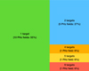 |
Fig. 1. Scheme representing the number of fields with one (green), two (light blue), four (orange), five (yellow), or nine (red) targets observed with IRAM 30-m. The area of each rectangle is proportional to the number of fields. |
The selection of the PHz fields for the IRAM observations is the result of ten different programs carried out during the past six years (2016−2021). The different number of targets per field is due to a change in the observing strategies throughout the project. Initially, we aimed at measuring one redshift per field. To this end, we selected fields with a bright (S350 μm > 75 mJy) red SPIRE source, and with a significant overdensity of SPIRE sources (Planck Collaboration XXXIX 2016). In those fields, the observing strategy was to observe the brightest red SPIRE source using a wide frequency coverage to search for a CO line. Subsequently, we either looked for an additional CO line in the detected targets and we observed additional SPIRE sources in the same field where we had a redshift. The goal of these additional observations was to detect other sources at the same redshift. For this purpose, we decreased the density flux limit at 350 μm from 75 mJy to 40 mJy and we gave priority to fields with sufficiently bright secondary targets and for which ancillary multiwavelength data were available. We observed three additional fields for specific reasons. First, we observed G073 because previous ALMA observations had serendipitously detected a CO line in this field (Kneissl et al. 2019). In G073, we targeted a CO-detected source (G073 03) with the goal of confirming the redshift by detecting another CO transition, and we also targeted another SPIRE source (G073 15) with the goal of identifying a CO line at the same redshift. Second, we observed G088 because of its significant overdensity of red SPIRE sources and the availability of HerMES/FLS data (Oliver et al. 2012). Last, we observed G237 because it contains a spectroscopically confirmed protocluster (Polletta et al. 2021; Koyama et al. 2021). We targeted a faint SPIRE source (G237 9741) because associated with a spectroscopic member, and the brightest red SPIRE source in the field (G237 962). All these additional targets are red, and four out of five also satisfy the flux limit criterion (S350 μm > 40 mJy). In one field (G112), a mistake was made in importing the coordinates during the observations and the pointing ended up being 17″ from the selected brightest SPIRE source and closer (at 12″) to another SPIRE source (G112 06) with S350 μm = 68 mJy, but not red. Thus, all the observed targets have S350 μm > 40 mJy, with the exception of G237 9741, and 17 have S350 μm > 75 mJy. In the following, we refer to all the selected targets as the PHz-IRAM sample.
In Fig. 2, we compare the SPIRE flux density at 350 μm of the PHz-IRAM sample (magenta and turquoise lines) with all SPIRE sources in the PHz fields in the region of the sky visible from the IRAM-30 m telescope site (δ ≳ −2°) and with Herschel coverage (1268 sources over 100 PHz fields). The submm colors of the selected targets (magenta and turquoise full circles and histograms) are compared with those of the parent sample (black circles, and gray filled histograms) in Fig. 3. The selected targets are among the brightest red SPIRE sources located in the PHz fields, and similar in terms of colors to the parent sample, with the only difference that they lack the bluest sources. In a handful of cases, S500/S350 is slightly lower than 0.6, the nominal threshold to classify a SPIRE source as red. This is the case of G112 06, selected because of a mistake in importing the coordinates, and of three sources (G073 03, G124 01, G124 02) where the flux density at 500 μm had not been correctly deblended at the time the sources were selected, and of one case (G131 15) where the target was a secondary target. In all these sources, the flux ratio is just below the threshold (0.55 ≤ S500/S350 < 0.6), as illustrated in Fig. 3.
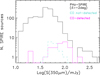 |
Fig. 2. SPIRE-350 μm flux density distribution of the targets observed with IRAM in this study (solid magenta line: CO-detected, and dashed turquoise line: CO not-detected), and of all SPIRE sources (black line) situated in the PHz fields in the region of the sky visible from the IRAM-30 m telescope site (δ ≳ −2°). |
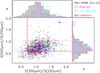 |
Fig. 3. SPIRE colors of the targets selected for IRAM observations (magenta full circles: CO-detected; turquoise full circles: IRAM observed but not CO-detected) and of all SPIRE sources (black circles) situated in the PHz fields in the region of the sky visible from the IRAM-30 m telescope site (δ ≥ −2°). The red lines enclose the region of red SPIRE colors. Top and right panels: submm color distributions normalized at the peak (gray: all PHz-SPIRE sources at δ ≥ −2; magenta: CO detected; cyan: CO not-detected). |
2.2. SPIRE source density
We characterize the SPIRE source overdensity of each targeted field following Clements et al. (2014) and Polletta et al. (2021). In brief, we built a density map considering all red SPIRE sources over a 20′×20′ region with > 1σ detection in all three SPIRE bands and a > 3σ detection in at least one band. For each selected SPIRE source, we computed a flux-weighted local density given by the distance distribution to the nearest five neighbors as:
![Mathematical equation: $$ \begin{aligned} \delta _i = \frac{W_i}{\pi \,d_{i,5}^2} \sum _{j=1}^{5} \exp \left[-0.5\left(\frac{d_{i,j}}{d_{i,5}}\right)^2\right], \end{aligned} $$](/articles/aa/full_html/2022/06/aa42255-21/aa42255-21-eq1.gif) (1)
(1)
where dij is the distance to the jth source, di, 5 is the distance from the ith source to the fifth nearest neighbor, and Wi is a weight given by the ratio between the ith source flux density at 350 μm and the sum of the 350 μm flux densities from all sources in the field (adapted from Clements et al. 2014). From the δi value of each SPIRE source, we created a map after convolution with a Gaussian kernel with a full width at half maximum (FWHM) of 3′. From the map, we then compute a mean background density (ρbck) as the 3σ clipped mean and the rms (ρrms).
A map of density contrast (δPHz)7 and one of overdensity significance8 were then obtained. In the overdensity significance map, we identified the region with adjacent pixels of a value greater than the maximum significance expressed by the nearest rounded-down integer number of σ (typically 5) and we computed the mean density contrast in this region. The maximum overdensity significance, the relative mean density contrast and region size for each PHz-IRAM field are reported in Table 1.
Red SPIRE overdensity.
Most of the selected fields exhibit significant (> 5σ) overdensities of red SPIRE sources. These overdensities are overlaid on the Herschel/SPIRE multiband images in Fig. 4. We also show the Planck red-excess contours, and the position of all SPIRE sources in the field. The SPIRE sources observed with IRAM, shown as large stars, are typically situated on the overdensity peak. The Planck red-excess emission, typically, matches well the SPIRE overdensity, but in some cases, the Planck red-excess contours are missing (G052, and G073) because those regions were masked in the 5′ resolution Planck maps utilized to extract the PHz catalog. In the remaining eight PHz fields that are not included in the official PHz source list (Planck Collaboration XXXIX 2016), a significant signal in the Planck red-excess map is still visible in six cases (i.e., in G124, but split in two less significant blobs, in G072, G112, G143, G131, and in G063), and no red-excess signal is present in the remaining two (i.e., G059, and G068). We refer to Appendix A in Planck Collaboration XXXIX (2016) for a more detailed comparison between the preliminary PHz extraction and the official catalog.
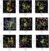 |
Fig. 4. 15′×15′ Herschel RGB (red: 500 μm, green: 350 μm, blue: 250 μm) maps centered on the IRAM observed PHz fields presented here. SPIRE sources are indicated with open circles (red: red submm colors; blue: blue submm colors; yellow: not detected in all three bands, thus preventing a color classification). IRAM targets are indicated with big stars (red: CO detection at similar redshift (i.e., Δz/(1 + z) < 0.02), cyan: CO detected, there is only one detection or multiple detections at different redshifts (i.e., Δz/(1 + z) > 0.02); white: CO not detected). Yellow contours represent the Planck red-excess emission (50%, 70%, and 90% of the maximum value). Green contours represent the overdensity significance of red SPIRE sources (starting at 3σ, with steps of 1σ). (a) G176. (b) G223. (c) G173. (d) G162. (e) G006. (f) G237. (g) G191. (h) G088. (i) G059. |
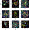 |
Fig. 4. continued. (a) G073. (b) G124. (c) G072. (d) G112. (e) G143. (f) G131. (g) G052. (h) G068. (i) G063. |
Previous works on the PHz sample have also quantified the density of red SPIRE and Spitzer/IRAC sources (Planck Collaboration XXVII 2015; Martinache et al. 2018). Unlike our method, the Herschel overdensity was computed only in the region where the Planck red-excess signal was greater than half of the maximum value. We did not apply the same methodology as we do not have the red-excess map for all selected sources, and the low resolution of the Planck maps introduces a broad uncertainty in determining the location of the submm emission. The method used by Martinache et al. (2018) is instead based on the density of red Spitzer/IRAC sources within 1′ from the brightest red Herschel source.
3. Observations and data reduction
Observations of the selected targets were carried out using the heterodyne Eight MIxer Receiver (EMIR) receiver (Carter et al. 2012) on the IRAM 30-m telescope. For the backends, we simultaneously used the Wideband Line Multiple Autocorrelator (WILMA, 2-MHz spectral resolution) and the fast Fourier Transform Spectrometer (FTS200, 200-kHz resolution). The program strategy was to carry out a blind redshift search in the 3 mm and 2 mm bands for the brightest red SPIRE source per PHz field. The frequency tuning was defined to search for the CO(3−2), or the CO(4−3) lines at z ≃ 2−3 ( = 86−115 GHz,
  = 115−154 GHz). Each source was observed for about 200 min, or longer in the case of a tentative detection. In the case of a line detection, an additional observation was carried out, when possible, to look for a second line to confirm the redshift. In a few fields, more than one source was observed with a tuning suited to find a line at the same redshift. The observed targets, project numbers, observing dates, selected bands, and integration times are listed in Tables A.2 and A.3.
We assume that the selected targets are smaller than the beam size at the observing frequencies. The FWHM of IRAM 30-m/EMIR is 27″ at 91 GHz, comparable to the Herschel-SPIRE beam at 350 μm9. Observations were performed in wobbler-switching mode with a throw of 80″–150″. For calibration, pointing, and focusing we used planets and bright quasars. Individual scans were 28−30 s long and we observed sets of 12 scans followed by a calibration. Data were reduced with the CLASS package in GILDAS (Gildas Team 2013). In a few cases, some scans were discarded because of an unstable baseline yielding different integration times in the two sub-bands. A baseline, computed as first-order polynomial of the spectrum, was subtracted from each individual scan. Scans were then averaged using the inverse of the square of the individual noise level as weight and smoothed to a velocity resolution given by the frequency and the line strength. We then applied the different point source conversion factors (in the range of 5.9−6.4 Jy K−1 depending on the optics and the frequency) to convert  [K] into a flux density [Jy]. The resulting co-added spectra were inspected to look for emission lines as multiple adjacent channels with signal higher than the rms in the nearby channels (∣Δv ∣ < 2800 km s−1) and then fitted with a single or a double Gaussian profile to measure the line position, the integrated line flux, and the line width (FWHM). We consider a line detected if the its signal-to-noise ratio (S/N) is greater than 4, but we report additional transitions with lower significance if their S/N is at least 2. The detected lines and derived parameters are listed in Table 2.
EMIR line detections.
In Fig. 5, we show the frequency coverage and integration time of each target, highlighting in magenta those that yielded a detection and in turquoise those where no line was detected. The integration time of some observations is not fixed but covers a broad range due to the removal of bad scans in some sub-bands or to the combination of observations with a slightly different tuning frequency. These are shown as boxes instead of straight lines in Fig. 5. The figure shows that a line is typically detected if the integration time is longer than 300 min or if the observation covers a broad frequency range.
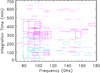 |
Fig. 5. EMIR integration time per frequency band of all observations. Boxes are shown in case some scans were not used in specific sub-bands. Observations relative to the same target are connected with dotted lines. The observations that yielded at least one CO line detection are shown in magenta, and those with no detections are shown in turquoise. |
In Fig. 6, we show the range of integration times used per target and the corresponding flux density at 350 μm. At a 350 μm flux density above 75 mJy all but two sources (88%) had at least one line detected. At fainter fluxes, a line was instead detected only in 37% of the cases. Although it is plausible that no line was present in the observed narrow frequency range, it is likely that in most of the cases, the lack of detection might be due to a combination of short integration time and source faintness instead of not having a line. In Figs. 2 and 3, we compare the submm fluxes and colors of the SPIRE sources that were CO detected with those that were not-detected. The latter are, on average, fainter and slightly redder. These properties indicate that they might be at slightly higher redshifts, but the difference would be small with respect to the wide redshift range of measured redshifts. We go on to see that most of the faintest targets were selected in fields where one or two primary sources had already been detected. The additional targets were observed with the goal of detecting a CO line at the same redshift. In the event of no line detection in ∼200 min from a first quick on-site data reduction, the observations were stopped to move onto a different target. These additional targets are typically 1.5−3 times fainter than the primary targets and would have required longer integrations. The EMIR spectra, together with the best-fit Gaussian components, are shown in Figs. B.1–B.3.
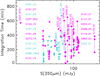 |
Fig. 6. EMIR integration time of all observations per source (full circle connected by a straight line) as a function of the source flux density at 350 μm. The source ID is noted. The observations that yielded at least one CO line detection are shown in magenta and those with no detections are shown in turquoise. |
4. Results
4.1. Line detections and redshifts
We detect 35 CO lines with signal-to-noise ratio (S/N)10 greater than 4 in 24 bright (S350 μm > 40 mJy, with one exception G237 962 which has S350 μm = 21 mJy) SPIRE sources in 14 PHz fields. Five additional CO lines are detected at a lower significance level, 2.2 < S/N ≤ 4.0, but are all confirmed by at least one reliable detection of a different transition. The lines’ transition, intensity, width (FWHM), rms, S/N, and corresponding redshift are listed in Table 2. The lines’ peak fluxes as a function of integration time, and of flux density at 350 μm are shown, respectively, in Figs. 7 and 8. The figures show a wide range of line fluxes, independently of the integration time, and of the submm brightness. This means that with our observations, we were able to measure, with the same integration time and for sources covering a limited range of submm fluxes (i.e., a factor of three in S350 μm), a broad range (a factor of ∼5) of CO line fluxes and, thus, of the gas masses. This large dynamic range in CO fluxes permits us to explore the intrinsic properties that influence the gas content in our sample.
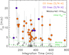 |
Fig. 7. Peak flux of the detected CO lines (full orange circles if S/N > 4.0, and purple if S/N ≤ 4.0) as a function of the integration time. The line rms is also shown (black triangles) and connected to the corresponding measured flux by a dotted vertical line. The expected trend of rmsline with the integration time is shown as dashed green line and the detection threshold of 4 × rmsline as dotted green line. The rmsline varies with channel width and depends on the line width. |
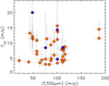 |
Fig. 8. Peak flux of the detected CO lines (full orange circles if S/N > 4.0, and purple if S/N ≤ 4.0) as a function of flux density at 350 μm. |
In eleven sources, we detected multiple (two in seven sources and three in the remaining four sources) CO transitions with consistent redshift, thus yielding a robust redshift estimate. A single line is instead detected in the remaining 13 sources. Because of the line strength and the expected redshift range, the line identification is straightforward in ten cases and, thus, the redshift estimate is reliable as a lower or higher redshift would be unlikely. In four cases (G006 01, G073 15, G131 15, and G063 02a), the line interpretation is ambiguous, we thus list the most plausible transitions and corresponding redshifts (see Flag = −1 in Table 2). The distribution in redshift derived from the CO lines is shown in Fig. 9. The measured secure redshifts span a range from 1.32 to 2.75, with an average of ⟨zCO⟩ = 2.25 ± 0.09. In the following analysis, we distinguish the parameters derived from the secure CO line identifications (red symbols in all the following figures) and those derived from the uncertain ones (blue symbols in all figures).
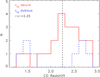 |
Fig. 9. Redshift distribution derived from secure (red) and dubious (blue) CO line identifications of 24 PHz sources. The dashed vertical black line represents the mean redshift, ⟨zCO⟩ = 2.25 ± 0.09, obtained from the secure identifications. |
In four out of the eight fields where more than one SPIRE source was observed, we detected CO emission from two SPIRE galaxies with consistent redshifts (G176 at z = 2.75, G059 at z = 2.36, G124 at z = 2.16, and G191 at z ≃ 2.6). In three of these fields, we targeted more than two sources (five in G176, nine in G191, and four in G124), but we either detected a CO line at a different redshift or no CO line at all. The number of observed, and detected sources and of those at similar redshift in each targeted field are summarized in Table 3. The lack of detection, in some cases, might have been due to insufficient integration times as these additional targets are 1.5−3 times fainter than the detected ones. In other three fields (G237, G073, and G131), the two detected targets were found at different redshifts, but additional redshift measurements from different observations in two of these fields have determined a significant concentration of sources at the same redshift. ALMA observations of G073 detect seven CO lines from five SPIRE sources at zCO ≃ 1.50 − 1.54 (Kneissl et al. 2019; Hill, priv. comm.). The ALMA observations detect two sources in the continuum associated with G073 15 (ALMA IDs 11, and 12 in Kneissl et al. 2019), but it is for only one (ALMA ID 12) that there is a CO detection at zCO = 1.50. We could not detect the expected CO line associated with this redshift because it falls exactly in a frequency gap of our observations, but we have a tentative detection at another redshift that might be associated with the other continuum source (ALMA ID 11). The optical and NIR spectroscopic observations in G237 have found a significant overdensity with 31 sources at z = 2.16−2.20 (Polletta et al. 2021), but most of them are not bright enough in the submm to be followed-up with the IRAM 30-m telescope. In the remaining field, G052, only one source was detected. In conclusion, IRAM can probably reveal only a few protocluster members, those with the largest gas reservoirs (see also Ivison et al. 2020). Some of these sources might be associated with multiple galaxies that can be individually detected only by high resolution sensitive mm observations. The effect of multiplicity is discussed in the next section.
IRAM observations summary.
4.2. Multiplicity
The possibility that multiple sources might contribute to a single SPIRE source emission is likely, especially in bright sources. It is widely known that bright SPIRE sources suffer from multiplicity, for instance, 9−23% of the SPIRE sources with bright density fluxes (S500 μm = 35 − 80 mJy) are multiple sources (Montaña et al. 2021; Scudder et al. 2016).
In our PHz-IRAM sample, we detected lines at two different redshifts in one source, G063 02. In Table 4, we report both measurements and add the suffixes “a” and “b” to the Herschel ID to differentiate them. In the following analysis, we adopt the full SPIRE emission for both sources and, thus, both their IR luminosity and SFR are shown as upper limits.
CO-derived properties.
There are also two SPIRE sources, G191 07 and G124 01, whose CO lines have double Gaussian profiles that could be due to two sources at similar redshifts (see Fig. B.2). In G124 01, both CO transitions (CO(3−2) and CO(4−3)) exhibit a double Gaussian profile. The mean difference in velocity between the two peaks (⟨zlow⟩ = 2.1522, and ⟨zhigh⟩ = 2.1540) is ⟨δv⟩ ∼ 171 km s−1, whereas the velocity difference between the two transitions is 26 km s−1 and 79 km s−1 for the low and the high z values, respectively. In G191 07, we detected three double peak CO lines (CO(3−2), CO(4−3), and CO(5−4)). In this source, ⟨zlow⟩ = 2.62237, and ⟨zhigh⟩ = 2.62514, thus the mean velocity difference between the two peaks is ⟨δv⟩ ∼ 229 km s−1, and the highest velocity differences across the three transitions are 84 km s−1 and 257 km s−1 for the low and the high z values, respectively.
The offset between the two peaks in both sources is larger than the difference across the three CO transitions, strongly favoring the double Gaussian solution in both G124 01, and G191 07. In addition, the line profile is not symmetric, with the two peaks having different intensities and widths, favoring kinematically distinct components that are suggestive of a merger system, instead of a rotating disk at the origin of these double peak profiles. Observations at high resolution would help to distinguish these two possible scenarios.
In the only PHz field for which high spatial resolution mm observations are available, namely, G073, Kneissl et al. (2019) found between one and four ALMA-detected objects in eight SPIRE sources. Subsequent ALMA observations of this field have found that two SPIRE sources contain two galaxies at the same redshift (Hill, priv. comm.).
In summary, we find evidence of multiplicity in 3 out of 24 sources (12%), consistent with previous studies (Montaña et al. 2021; Scudder et al. 2016). The 350 μm flux densities of these three sources range from 57 to 116 mJy, which are consistent with the peak of the flux density distribution and they are not the brightest examples. We cannot rule out the possibility that other sources might be multiple, but the limited frequency coverage and integration times of our IRAM observations might have not revealed sources at different redshifts or those with fainter CO emission.
4.3. Considering whether PHz fields contain high-z proto-structures
The main goal of the EMIR observations was to determine whether the PHz fields contain high-z structures. Finding multiple sources at similar redshifts (∣Δv ∣ < 2000 (1 + ⟨z⟩) km s−1; see Eisenhardt et al. 2008) would support this hypothesis.
We measured redshifts for multiple Herschel sources in projected proximity in eight PHz fields. In half of those fields, we detected two objects at similar redshifts. In the following, we refer to these as the structures’ redshifts. In two of the fields with two sources at the same redshift, G191 and G124, two SPIRE sources have a double peak CO line implying two sources at the same redshifts. Thus, in these two fields, we found three sources at consistent redshift associated with two distinct SPIRE sources.
In three fields more than two SPIRE sources have been observed (four in G124, five in G176, and nine in G191), but out of the 18 targets in this subset: 6 are at the structure redshift, 3 are at different redshifts, and no redshift was measured in the remaining nine. The number of observed, and detected sources and of those at similar redshift in each targeted field are listed in Table 3. The lack of CO detection can be in part explained by insufficient exposure times. Indeed the primary targets that led the first CO-detections in each field were a factor of 2−3 brighter than the secondary targets and were usually observed with 1.5−3 times longer exposure times. This observing strategy was defined to find CO line detections at the same redshift as the primary targets. A line was successfully detected in 10 out of 20 secondary targets. In the remaining cases, we cannot rule out the possibility that the sources are at the same redshift as the primary target as the achieved depth might have been insufficient to detect a CO line in those additional fainter targets.
These results, despite their being based only on eight fields, provide support to the hypothesis that the PHz fields contain overdensities of DSFGs at z ≃ 2 − 3, but also indicate that DSFGs situated along the line of sight contribute to the Planck signal. We can thus conclude that the Planck selection technique is efficient in finding overdensities of highly star-forming systems at z ≃ 2, but the measured Planck signal is also affected by line of sight projections, as predicted by Miller et al. (2015) and Negrello et al. (2017).
4.4. Far-infrared properties: Luminosities, dust temperatures, and SFRs
With the CO-derived redshifts, accurate infrared luminosities can be measured for all CO-detected SPIRE sources. The total (8−1000 μm) IR luminosities (LIR), dust temperatures (Tdust), and SFRs are estimated by fitting the SPIRE data with single-temperature modified blackbody models. SCUBA-2 data at 850 μm are also included in two cases (G006 01, and G068 02; MacKenzie et al. 2017). Fits were performed using the cmcirsed package (Casey 2012) and assuming the CO-derived redshift and a dust emissivity-index β equal to 1.8 (Cortese et al. 2014; Pokhrel et al. 2016). The code returns also the uncertainties on LIR and Tdust. The quoted uncertainties in LIR do not account for the uncertainty in the redshift as it is negligible compared with the uncertainties associated with the photometric points and the best-fit model. From the IR luminosities, SFR estimates are derived assuming the relationship in Kennicutt (1998), modified for a Chabrier IMF (Chabrier 2003), SFR/(M⊙ yr−1) = 9.5 × 10⁻¹¹LIR/L⊙.
The far-IR derived parameters LIR, Tdust, and SFR are listed in Table 5. Infrared luminosities as a function of redshift are shown in Fig. 10. In the case of dubious line identifications (four cases), we show both redshifts and IR luminosities in the figure. All detected targets are classified as ultraluminous IR galaxies (ULIRGs; LIR ≥ 1012 L⊙; Sanders et al. 1988), and 50% are hyperluminous IR galaxies (HyLIRGs; LIR ≥ 1013 L⊙) with consequently large (≳100 M⊙ yr−1) SFRs (see Fig. 10). The highest SFR (≳3000 M⊙ yr−1) is measured in G176 01, which is the highest redshift source together with G176 02 (both at zCO = 2.75). The average SFR, considering only the secure CO identifications, is 1043 ± 157 M⊙ yr−1. The large IR luminosities are due to the sample selection, as illustrated by the dashed line corresponding to the IR luminosity of a source with S350 μm = 40 mJy and Tdust = 30 K.
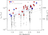 |
Fig. 10. Total IR (8−1000 μm) luminosity or SFR as a function of redshift for the PHz-IRAM sources (full red stars for secure line identifications and full blue stars for uncertain line identifications) and for 1.4 < z < 3.1 cluster and protocluster members from the literature (gray triangles and crosses). In the case of multiple EMIR detections associated with the same SPIRE source, an upper limit to LIR was reported with a downward pointing arrow. Blue stars connected with a solid blue line refer to the same source and to two possible redshifts. The black dashed line represents the total IR luminosity of a source with S(350 μm) = 40 mJy and Tdust = 30 K (derived using the cmcirsed package; Casey 2012) corresponding to the selection of the majority of the PHz-IRAM targets. The dotted line is the same LIR limit scaled by −0.2 dex and used to select a subset of cluster and protocluster members from the literature for comparison (gray triangles). |
Far-infrared properties of the CO detected sources.
In Fig. 10, we also show, for comparison, the IR luminosities of cluster and protocluster members from the literature with 1.4 < z < 3.1 and for which CO observations are available (see full list in Table C.1). The IR luminosities from the literature sample extend to much lower values (see also Table C.1) than the PHz-IRAM sample. For the purpose of a proper comparison, we selected only a subset of the literature sources with IR luminosities greater than our limit minus 0.2 dex (see dotted line in Fig. 10). This choice, although it might appear somewhat arbitrary, does take into account the uncertainty on the LIR values and yields a sample size (41 sources) that is well suited for a comparison.
In Fig. 11, we show the estimated dust temperatures as a function of IR luminosities for our sources. The Tdust − LIR relations derived for local IR-selected galaxies (Chapman et al. 2003), for z ≃ 2 SMGs (Chapman et al. 2005), and for z < 1.5 SPIRE sources (Symeonidis et al. 2013) are also shown for comparison. We also report the dust temperatures expected for main sequence (MS: SFR–ℳ relation of SFGs; see e.g., Speagle et al. 2014) galaxies in the redshift range of our PHz-IRAM sources (1.3 < z < 2.8) based on the relation between Tdust and the offset from the MS reported by Magnelli et al. (2014). In galaxies, the intensity of the radiation field increases with lookback time (e.g., Magdis et al. 2012; Huang et al. 2014; Béthermin et al. 2015) along with a concurrent rise in dust temperatures. Indeed local galaxies have typically colder dust than those at higher redshift (e.g., Tdust ∼ 20 − 55 K in local U/LIRGs, and 25−60 K in those at z ≃ 2 − 2.5, whereas normal SFGs have Tdust ∼ 20 K at z ∼ 0, and Tdust ≳ 30 K at z ≥ 1; Clements et al. 2018; Magdis et al. 2010; Symeonidis & Page 2018; Cortese et al. 2014).
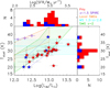 |
Fig. 11. Main panel: dust temperature as a function of the IR (8−1000 μm) luminosity for the PHz-IRAM sources (full stars, red for secure CO line identifications, and blue for the uncertain ones). The shaded orange area shows the local Tdust − LIR relation derived by Chapman et al. (2003), linearly extrapolated to 1013 L⊙. The shaded cyan area shows the range of dust temperatures for main sequence galaxies in the redshift range of the PHz-IRAM sources (1.3 < z < 2.8) according to the relation found by Magnelli et al. (2014), and extended to LIR > 1013 L⊙. The shaded green area presents results for z ≃ 2 SMGs from Chapman et al. (2005). The purple diamonds represent the relation found for z < 1.5 SPIRE sources by Symeonidis et al. (2013). Top and right panels: distributions of SFR (and IR luminosity) and dust temperature, respectively, for all PHz-IRAM sources. |
The PHz-IRAM sources, with an average of ⟨Tdust⟩=(29.2 ± 0.9) K exhibit dust temperatures consistent with those observed in MS galaxies at similar redshifts, but colder than those typical of local SMGs and z < 1.5 SPIRE sources. Compared to the z ≃ 2 SMG population, there is some overlap, but more on the low Tdust–high LIR side. We point out that higher β values would yield lower dust temperatures, but even if we assume β = 1.5 as in Chapman et al. (2005), the observed temperature offset will still be present. We consider the possibility that this difference might be a consequence of fitting the submm SED without data at ≥850 μm which are typically available for SMGs. However, in the two cases where a SCUBA2 850 μm flux measurement is available, namely, G006 01 and G068 02, the estimated dust temperatures are similarly low. We thus conclude that our sources are characterized by lower dust temperatures, by ∼5 K on average, than the z ≃ 2 SMG population. Our results on the dust temperature indicate that our PHz-IRAM sources are similar to those observed in normal SFGs at similar redshifts.
4.5. CO spectral line energy distribution
The shape of the CO spectral line energy distribution (SLED) is linked to the underlying molecular gas density and kinetic temperature (see e.g., Schirm et al. 2014; Daddi et al. 2015; Cañameras et al. 2018). Typically, the warmer and denser the molecular gas, the more populated the upper levels, along with a SLED rising faster with the line frequency. The CO SLED shape depends on the portion of dense gas and can thus indicate the star-forming mode (merger versus disk; Daddi et al. 2010; Zhang et al. 2014). Thus, studying the CO excitation properties offers a means to investigate what powers the elevated SFRs of our sources. For example, merger-driven starburst galaxies are much more highly excited in their high-J CO transitions than disk galaxies (Weiß et al. 2007; Papadopoulos et al. 2012). Lower densities and temperatures (Tkin ∼ 15 − 20 K, log(nH2/cm−3) ∼ 3.0; Carilli & Walter 2013) yield SLEDs that peak at lower transition values, similar to the Milky Way (peak at Jup = 3).
Since we have observed, at the most, three CO transitions in the same source, we cannot build a full CO SLED, but we can build portions of the CO SLED and compare them with those observed in other sources from the literature. In this analysis, we do not consider G059 03 because only one out of the three CO lines is well detected. In the case of sources with double peak lines (G191 07a, G191 07b, G124 01a, and G124 01b), we show the CO SLED derived from the single Gaussian fit and for each component of the double Gaussian fit. In Fig. 12, we show portions of the CO SLEDs of ten PHz-IRAM sources for which multiple CO transitions are detected, compared with those typical of SMGs, quasi stellar objects (QSO), color-selected SFGs (CSGs), BzK-selected galaxies, and to that of the starburst galaxy M 82 and of the Milky Way (Carilli & Walter 2013; Bothwell et al. 2013).
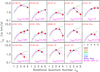 |
Fig. 12. CO SLEDs of the PHz-IRAM sources (full red circles connected by a black solid line). The CO SLEDs of different types of galaxies normalized to the observed CO(3−2) intensity of each PHz-IRAM source are shown for comparison in each panel as dotted lines: the Milky Way (purple; Fixsen et al. 1999); SMGs (orange), QSO (brown), the prototypical starburst galaxy M 82 (green), and color-selected SFGs (CSG; blue) from Carilli & Walter (2013); and BzK galaxies at z ∼ 1.5 (cyan) from Daddi et al. (2015). The solid magenta line in each panel shows the SLED model from Narayanan & Krumholz (2014) obtained assuming the annotated SFR density in M⊙ yr−1 kpc−2. |
The CO SLEDs of our sources peak, typically, at low rotational quantum numbers, similar to the Milky Way and differently from the SMGs at similar redshifts ( = 3,
= 3,  ; Carilli & Walter 2013). In eight sources, or 80% of the sources with measured line ratios, the CO SLED peaks at Jup = 3. There are only two exceptions, G191 07 (including 07a, and 07b) and G176 02, where the peak is at Jup ≥ 4, which is consistent with what is observed in SMGs at similar redshifts. These results suggest that the molecular gas in the most PHz-IRAM sources must be at low densities, cold (T ∼ 10 − 15 K), and at low-excitation. To investigate whether these properties are observed in other protoclusters, we searched for protocluster members from the literature with multiple CO transitions. We found 21 sources from five protoclusters (HXMM20, 4C 23.56, BOSS 1441, GOODS-N, and Cl J1449+0856; Gómez-Guijarro et al. 2019; Lee et al. 2017, 2019; Casey 2016; Coogan et al. 2018). Their CO SLEDs, compared with those from the same classes of galaxies used earlier, are shown in Fig. 13. The CO properties of these sources are listed in Table C.1. For this analysis, we included also sources that do not satisfy the IR luminosity selection criterion applied earlier with the aim of having the largest and most complete comparison sample, but we have flagged them in the figure (see source name in parentheses).
 |
Fig. 13. CO SLEDs of protocluster members from the literature (full pink circles connected by black lines; Coogan et al. 2018; Casey 2016; Lee et al. 2017, 2019; Gómez-Guijarro et al. 2019) compared with the CO SLED of different types or sources (dotted lines of color as in Fig. 12). Downward pointing arrows indicate upper limits. The protocluster and source names are annotated (see Table C.1). Source names between parentheses are those that do not satisfy the IR luminosity selection criterion. |
In eight cases, the available CO data are insufficient to constrain the SLED peak because there are only transitions with Jup ≤ 3 that are are available. In the remaining 13 cases where higher transitions are available, low excitation SLEDs are observed in seven sources (DSFGJ123711+621331, HAE16, HAE10, A2, HAE8, HAE4, and B1), a high excitation SLED is observed in one case (HAE9) and a SLED with intermediate excitation properties in the remaining five sources. Thus, half of the members from the literature have CO excitation properties as in normal SFGs. Similar conclusions were drawn by Coogan et al. (2018), based on the CO SLED analysis of the Cl J1449+0856 cluster members.
To further investigate this result and its plausible implications, we resorted to theoretical models. By combining numerical simulations with molecular line radiative transfer calculations, Narayanan & Krumholz (2014) developed a model for the physical parameters that drive variations in the CO SLEDs of galaxies. They found that the shape of the SLED is determined by the gas density, temperature, and optical depth distributions and that these quantities are correlated with a galaxy mean star formation rate surface density (ΣSFR). Based on this model, we derived the ΣSFR values that optimally reproduce the observed CO SLEDs. The predicted SLEDs, obtained assuming the relation for unresolved sources (see Eq. (19) and Table 3 in Narayanan & Krumholz 2014) are shown in Fig. 12 after normalizing them at the observed CO(3−2) intensity, and the derived ΣSFR are reported in Table 6. In four PHz-IRAM sources (G191 01, G124 01, G124 01b, G124 15, and G131 01), the measured SLED is not well reproduced by the model. Since the parametrized form that links the line ratios to the SFR surface density is valid only for ΣSFR ≥ 1.5 × 10⁻² M⊙ yr−1 kpc−2, and the peak of the SLED decreases for lower ΣSFR, the lack of a best-fit points to ΣSFR values that are lower than the minimum assumed by the model. Such a minimum is not physically motivated, but it is due to the impossibility of parameterizing the model relation with the same analytical expression at lower ΣSFR.
SFR and molecular gas density and extent.
From the estimated SFR surface brightness and the measured SFRs (see Table 5), we can derive the size of the star-forming region. Based on the assumption that the observed SFR is produced by the measured molecular gas mass and that they have the same extent, we can also derive a molecular gas density. All these values are reported in Table 6. Based on the prescription between line ratios and ΣSFR parameterized by Narayanan & Krumholz (2014), the size of the star-forming region or molecular gas extent would be implausibly large (Rgas ≳ 70 kpc) in most of the cases. Thus, we conclude that it is either the model or the model parameters, such as the gas density and temperature, that are not appropriate for our sources or, alternatively, our SLEDs are not correct. The latter could be the case if dust obscuration is present as it might depress the emission in the high transitions (Papadopoulos et al. 2010). It is also possible that the low transition peak of the observed SLEDs is artificially produced by the variation of the beam size with wavelength (i.e., the IRAM 30-m main beam is 29″ at 86 GHz, and 16″ at 145 GHz)11 in the case of extended or contaminated sources or of inaccurate pointing during the observations. Gravitational lensing can also produce a larger magnification of the diffuse gas emission seen in the low transitions than that coming from the compact gas traced by higher transitions, artificially producing a low peak in the CO SLED (see Hezaveh et al. 2012). This possibility is further discussed in Sect. 5.4. To investigate these results in depth, it would be necessary to obtain CO observations at a higher spatial resolution. Such observations would provide the size of the molecular gas distribution and reveal whether multiple sources are present in the EMIR low-frequency beam and enhancing the CO flux at smaller frequencies or whether some of our sources are affected by gravitational lensing.
4.6. CO luminosities
The CO luminosities are calculated following Solomon et al. (1997):
 (2)
(2)
where SCO(ΔV) is the line intensity derived from the Gaussian fit and νobs is the line observed frequency (see Table 2). The derived CO luminosities are then converted to the CO(1−0) luminosity,  , using the brightness temperature ratios measured for SMGs by Bothwell et al. (2013)12.
Since the CO SLEDs of the PHz-IRAM sources are not always consistent with those typical of SMGs, this choice might introduce large uncertainties on  and on the gas mass estimate. The choice of a different SLED would yield a
  value a factor of ∼1.8 higher (
 = 0.93/0.52 = 1.8), or ∼0.5 smaller (
 = 0.27/0.52 = 0.5) when derived from CO(3−2). Larger uncertainties would result when using luminosities from CO transitions with Jup > 3. In the case of multiple detected CO lines, we thus chose the line at the lowest transition – CO(3−2) in most of the cases – to derive
  and minimize the uncertainty associated with the brightness temperature ratios. In two cases (G059 01 and G059 03), we preferred a higher transition, CO(4−3), because it is more significantly detected than CO(3−2). The derived luminosities are listed in Table 4 and plotted as a function of redshift in Fig. 14. In all the figures where
  is shown, we report a unique value per source in the case of secure line identification and two values in case the line is not univocally identified.
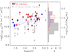 |
Fig. 14. CO(1−0) luminosity as a function of redshift for the PHz-IRAM sources. Symbols are the same as in Fig. 10. The purple and magenta curves show the expected |

For comparison, we include the CO(1−0) luminosities from cluster and protocluster members from the literature at 1.4 < z < 3.1 after applying the LIR cut (see Table C.1). The distributions of CO(1−0) luminosities for the PHz-IRAM sources and the literature sample are shown on the right hand panel of Fig. 14. The PHz CO(1−0) luminosities are, on average, 0.4 dex higher than those of the literature sources. From  , it is possible to derive the molecular gas mass through a conversion factor, αCO, that depends on the physical properties of the gas. The αCO for normal SFGs at high-z is typically 3.5 (Magdis et al. 2017). The molecular gas masses derived from
  assuming αCO = 3.5 (see Sect. 4.9) are shown on the right hand axis in Fig. 14. The PHz sources are among the most luminous and, thus with the largest gas reservoirs, CO-detected galaxies found in overdense regions at 1.4 < z < 3.1. This result can be in part explained by the selection bias in favor of the brightest submm sources targeted and detected per field, as illustrated by the dashed and dotted curves shown in the figure. On the other hand, there must also be an intrinsic property associated with the extreme luminosities and gas masses found in our sources because of the wide range of CO(1−0) luminosities observed at fixed IR luminosity.
4.7. PHz-IRAM sources: Normal SFGs or starbursts
Star-forming galaxies follow a relation between the CO(1−0) luminosity and LIR that describes, in observable terms, the relationship between the luminosity due to star formation and the total gas content. This relation is different for normal SFGs and starburst galaxies, with the latter having  smaller by 0.46 dex, on average, at fixed IR luminosity than normal SFGs (as formulated by Sargent et al. 2014)13. In Fig. 15, we show the relations for SFGs and starburst galaxies, and the values derived for our PHz-IRAM sources and for the cluster and protocluster galaxies drawn from the literature. Both the PHz-IRAM sources, and those drawn from the literature agree with the scaling relations, although with a large scatter. Indeed at fixed IR luminosity,
  can vary by up to a factor of five in our sample, compared with the factor of almost three that separates normal SFGs from starburst galaxies. The large scatter means that the SFE varies across the sample, but some of the scatter might be also due to a multiplicity effect. The IR luminosity might be overestimated because derived assuming that all the SPIRE flux is emitted by the CO source. The same might be true for the CO luminosity if multiple sources at the same redshift are present.
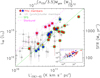 |
Fig. 15. Total IR (8−1000 μm) luminosity or SFR as a function of CO(1−0) luminosity for the PHz-IRAM sources and for 1.4 < z < 3.1 cluster and protocluster members from the literature (same symbols as in Fig. 14). The protocluster massive spiral HAE229 (Dannerbauer et al. 2017) is shown as full gold triangle. The solid green line and the dashed magenta line represent, respectively, the average relations for normal SFGs and starburst galaxies (Sargent et al. 2014). Open magenta or green squares are overplotted over the PHz sources classified as starburst, or normal SFGs based on the agreement with the drawn relations. In the inset, we show the same graph and data, but extended to lower luminosities and include a sample of CO-detected normal SFGs at z = 1.4−2.4 (lilac open circles; Daddi et al. 2010; Tacconi et al. 2013). |
Based on the comparison with the two relations, we classified our sources as normal SFGs if log( ) > log(
 )SFG − 0.3, where
  )SFG is the expected
  assuming the SFG relation (Sargent et al. 2014) at the observed LIR, and starburst if log(
 ) < log(
 )SFG − 0.3. Normal SFGs and starbursts are identified in the figure with, respectively, green and magenta open squares. Most of our sources (16/20 sources or 80% of those with secure CO identification) are consistent with or below the normal SFGs relation, and four (20%) are in the starburst locus. Those classified as starbursts (G176 02, G173 01, G059 03, and G124 03) are all at high redshifts (z > 2.3), but other sources at similarly high redshift are classified as normal SFGs. If we consider the sources with double peak lines, G191 07, and G124 01, as made of two separate galaxies, we find that in one case (G124 01), both galaxies (01a, and 01b) would be classified as starbursts. This is, however, the case if we do not deblend the SPIRE flux. If the IR luminosity is scaled by their contribution to the total CO luminosity their values would be consistent with the SFG relation. The starburst galaxies represent 20 ± 10% (4 out of 20 sources) of the PHz-IRAM sources with secure line identifications. If we interpret this percentage as the starburst phase timescale in the PHz-IRAM sample, we can infer that this phase lasts ∼20% of the galaxy lifetime. Thus, during most of their lifetime the bright PHz sources behave similar to normal SFGs.
Among the sources from the literature, a larger percentage, namely, 32% (13 out of 41 sources) falls in the starburst locus compared with our sample, but the majority agree with the normal SFG relation. It is interesting to point out that although the PHz-IRAM SFGs are in agreement with the normal SFG relation, their luminosities are systematically greater than measured in typical SFGs at similar redshifts. In the inset of Fig. 15, we show the luminosities of the sub-sample of normal SFGs at z = 1.4−2.4 used by Sargent et al. (2014) to derive the normal SFG relation. This includes 14 galaxies from the PHIBSS sample (Tacconi et al. 2013), and 6 of the BzK galaxies (Daddi et al. 2010). Our PHz-IRAM sources occupy the high luminosity tail of the luminosity distribution observed in the normal SFG sample, with average values of IR and CO luminosities being eight and five times larger, respectively, than those relative to the normal SFG sample. With respect to the protocluster SFG members drawn from the literature, the PHz-IRAM sources exhibit IR and CO luminosities that are, on average, only a factor of two higher. A factor of two is not significant considering the scatter in the luminosity distributions14. Thus, our selection of bright red submm galaxies yields mostly normal SFGs, but with greater IR and CO luminosities and, thus, greater SFRs and gas masses than typically observed in normal SFGs and in other protocluster members at similar redshifts.
4.8. CO excitation and LIR– relation
In Sect. 4.5, we show how we were able to identify the sources in our sample with highly excited CO, as expected in starburst galaxies. It is thus interesting to compare the classification based on the LIR– relation, with the CO excitation level. Among the four sources classified as starbursts, the CO SLED has been measured for only G176 02, and G173 01. The CO SLED of G176 02 (peak at Jup = 5) is consistent with a starburst classification, G173 01 has, instead, a line ratio ICO(5 − 4)/ICO(3 − 2) = 0.61 ± 0.25, consistent with the MW CO SLED (i.e., ICO(5 − 4)/ICO(3 − 2) = 0.82), and much lower than observed in starburst galaxies (e.g., ICO(5 − 4)/ICO(3 − 2) = 2.24 in the prototypical starburst M 82). For the other two starburst galaxies, the CO SLED is not constrained. Conversely, the only other source with a highly excited CO SLED, G191 07, is consistent with the normal SFG
  relation. In summary, out of the ten sources for which the CO SLED is measured, one is classified starburst and has a highly excited CO SLED (G176 02), eight are classified normal SFGs and have a CO SLED consistent with low excitation, and one is classified starburst, but is not highly excited (G173 01). We remind the reader that the IR luminosity of our sources might be overestimated in the case of multiplicity affecting the measured Herschel emission and that in such a case the true LIR could be lower moving a source towards the normal SFG relation. We can thus conclude that the classification based on the
  diagram aptly matches the gas excitation level.
4.9. Molecular gas masses and depletion times
Gas masses depend on the assumed CO SLED as this provides the intensity of the CO(1−0) line from higher transitions and on the CO–H2 conversion factor (αCO = MH2/ ) to convert the CO gas mass into H2 mass (see review by Bolatto et al. 2013). As discussed earlier, the brightness ratios adopted for our sources to derive the CO(1−0) luminosity from that at higher transitions, are those observed in SMGs (Bothwell et al. 2013), even if the CO SLEDs of our sources seem to differ from those. On the other hand, assuming brightness ratios typical of normal SFGs, such as the Milky Way, would yield CO(1−0) luminosities and gas masses that are ∼2 times larger (Carilli & Walter 2013). Since our values are already higher than those typically observed in other z ∼ 2 galaxies, we prefer to use the standard SMG ratios that are also commonly adopted in the literature and more suited for a comparison with those samples.
Regarding the CO–H2 conversion factor, in normal SFGs such as the Milky Way, αCO is ∼4.36 (including the contribution of Helium to the molecular gas mass) and for starburst galaxies and mergers, it is typically ∼0.8 (Bolatto et al. 2013). Studies of the molecular gas at high redshifts have shown that this dichotomy breaks down and that αCO covers a broad and continuous range of values between ∼0.2 and ∼10 M⊙ pc−2 (K km s−1)−1 (Tacconi et al. 2008; Casey et al. 2014). The αCO value decreases with the offset from the MS relation that links a galaxy SFR with its stellar mass (see Eq. (2) in Castignani et al. 2020). Thus, galaxies above the MS, such as the starburst galaxies, have smaller αCO values.
The αCO value depends also on the galaxy gas metallicity (Genzel et al. 2012; Inoue et al. 2021). Since we do not have estimates of stellar mass nor of gas-phase metallicity for our sources, we assume a solar metallicity for all sources and adopt αCO = 3.5 M⊙ pc−2 (K km s−1)−1, as reported in Magdis et al. (2017) for normal SFGs with solar metallicity at z ∼ 2. For the PHz classified as starbursts based on their position in the  diagram (see previous section), we assume the same αCO value for consistency within the PHz-IRAM sample. The estimated gas masses assuming αCO = 3.5 M⊙ pc−2 (K km s−1)−1 are listed in Table 4.
From the gas masses, we can compute the star formation efficiency (SFE) given by the ratio between the SFR and the molecular gas mass. The SFE shows how efficiently the molecular gas mass is converted into stars. The estimated SFEs for our sources as a function of gas mass are compared with those from the literature in Fig. 16.
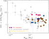 |
Fig. 16. Star formation efficiency (SFE) of the PHz-IRAM sources as a function of gas mass. Symbols as in Fig. 15. |
The PHz-IRAM sources exhibit a broad range of SFEs and gas masses, both spanning 1 dex. The broad range of SFEs is probably a reflection of the extent in redshifts, SFRs, and gas masses observed in our sample, although there is no clear correlation between the SFE and those quantities. The only noticeable features are that the sources with the highest SFE values are all classified as starburst and the least efficient sources are among those with the largest gas masses (Mgas > 3 × 10¹¹ M⊙).
The inverse of the SFE, defined as the molecular gas depletion time, τdep ≡ Mgas/SFR, represents the timescale required to exhaust the molecular gas mass with the current SFR. Normal SFGs at high redshifts (z ≳ 1.5) are characterized by τdep ≳ 0.45 Gyr (Tacconi et al. 2013; Saintonge et al. 2013), slightly decreasing at higher redshifts (1.5 × (1 + z)−1.5 < τdep < 1.5 × (1 + z)−1; Saintonge et al. 2013). In Fig. 17, we show the estimated gas depletion times of our PHz-IRAM sources (see values in Table 5). We compared them with the selected protocluster sample from the literature and with the aforementioned evolutionary track for normal SFGs (Saintonge et al. 2013).
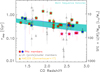 |
Fig. 17. Estimated depletion times of the PHz-IRAM sources as a function of redshift. Symbols as in Fig. 15. The turquoise region is the locus of normal SFGs (Saintonge et al. 2013). |
The average depletion time of the PHz-IRAM sources is ⟨τdep⟩ = 0.47 ± 0.07 Gyr. Similar depletion times are observed in the protoclusters drawn from the literature. The large uncertainties associated with these estimates do not allow us to analyze any trend with the redshift. Indeed, they are all consistent with the average value, and with the normal SFGs’ evolutionary track.
Assuming the current SFR and 100% conversion of gas into stars with no refueling, we can estimate by which redshift the molecular gas would be fully consumed. The estimated depletion redshifts of the sources with a secure redshift, listed in Table 5 and shown in Fig. 18, range from 1.17 to 2.56 and have a mean value of 1.93 ± 0.34. These redshifts are consistent with the epoch of build up of the passive galaxy population in clusters (e.g., Pallero et al. 2019).
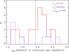 |
Fig. 18. Estimated redshift by which the molecular gas would be depleted (zdep) assuming the current SFR and 100% conversion of gas into stars with no refueling (red solid line: sources with secure redshift, blue dashed line: sources with uncertain redshift). The vertical black dashed line represents the mean zdep value derived from the sources with secure redshifts. |
4.10. CO kinematics
The CO line emission traces the kinematics of the potential well in which a galaxy’s molecular gas lies, and it is also affected by inclination and dispersion effects. In particular, the CO line width is sensitive to both the dynamical mass and inclination effects, whereas the luminosity ( ) is sensitive to the total molecular gas mass (see Sect. 4.9). In Fig. 19, we show the CO(1−0) luminosity derived from the lowest transition line for each target with secure redshift as a function of line width. For each line, we report the measured width, whereas the luminosity is converted to the CO(1−0) luminosity using the line ratios from Bothwell et al. (2013). We also show for comparison the relation between the CO(1−0) luminosity and FWHM derived for unlensed CO-detected SMGs by Bothwell et al. (2013), the values measured in several cluster and protocluster members at 1.4 < z < 3.1 from the literature (see Table C.1), and those measured in lensed SFGs at 1.4 < z < 3.0 from the HATLAS, GEMS, SPT, and PCCS samples, and in intermediate mass or low LIR lensed SFGs (Harris et al. 2012; Saintonge et al. 2013; Dessauges-Zavadsky et al. 2015; Cañameras et al. 2015; Aravena et al. 2016; Yang et al. 2017; Harrington et al. 2018; Solimano et al. 2021). We also report the median values of each subsample15.
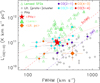 |
Fig. 19.
|

The PHz-IRAM sources show a relatively flat distribution of  with line widths spanning a wide range (FWHM ∼ 134 − 839 km s−1). They do not follow the relation between
  and FWHM observed in the SMGs and in the protocluster members from the literature (
 ; see dashed purple line in Fig. 19; Bothwell et al. 2013). Lensed SMGs are known for exhibiting a similar flat trend (Aravena et al. 2016; Yang et al. 2017). Such a behavior has been interpreted as lensing magnification acting on a population with intrinsically steep number counts and detected above a constant CO flux threshold (Harris et al. 2012). It is relevant to point out that our lens compilation, which includes lensed SFGs with low IR luminosities (Dessauges-Zavadsky et al. 2015), at intermediate masses (Solimano et al. 2021), and with extreme IR luminosities (Harrington et al. 2018) produces a different distribution than the flat one reported in some previous works. An analysis of the
  –FWHM relation in lensed SFGs is beyond the scope of this work, but understanding the origin of this flat trend might help to interpret our sample as well, and vice versa, even if our sources are not affected by lensing. Another striking difference compared with the protocluster sample from the literature is the significant percentage (24%) of sources with narrow (FWHM < 200 km s−1) lines.
To explain the observed linewidths, we consider the parameters that influence them, the gas mass density profile, extent, and velocity dispersion. The relation between  and the linewidth (FWHM) can be written as:
 (3)
(3)
where C is a constant parameterizing the kinematics of the galaxy that can assume values from ≤1 to ≥5, with the latter being the case of a uniform sphere and lower values for disk distributions (see e.g., Erb et al. 2006a), G is the gravitational constant, and R is the radius of the CO(1−0) emission region (e.g., 7 kpc; Ivison et al. 2011; Bothwell et al. 2013). High-z SMGs follow this relation assuming αCO = 1.36, R = 7 kpc, and C = 2. Their scatter around this relation is small ( ; Bothwell et al. 2013) implying compact sizes and regular gas motions. The PHz sources are, on average, on a relation shifted towards larger luminosities by a factor of 5 (see red dashed line in Fig. 19), implying larger C, and R values, and thus more random motions or large inclinations in the case of disks, and larger sizes.
Taking into account the different αCO factors assumed for our sources and for the SMGs, we can write CPHz × RPHz as  ). Replacing CSMG, RSMG, and the different αCO factors with the appropriate values, we obtain CPHz × RPHz = 180. Assuming the highest C value, that is 5, valid for a uniform sphere, RPHz would be ∼36 kpc. The derived RPHz value is plausible, but unusually large, compared with the sizes of the molecular gas reservoirs in high-redshift galaxies (i.e., < 25 kpc; Riechers 2011; Sharon et al. 2016; Keating et al. 2020). Interestingly, an extended (R ≃ 20 kpc) molecular gas distribution has been reported in another protocluster galaxy, HAE229 (Dannerbauer et al. 2017), but as a rotating disk.
It is important to point out that the PHz-IRAM sources do not lie on the expected relation, even if scaled by a factor of 5. The relation that best describes our sample has a slope of 0.87 ± 0.07 (i.e., log( ) ∝ (0.87 ± 0.07) × log(FWHM); see red dotted line in Fig. 19), instead of a slope of 2 as expected for a rotating disk (see Eq. (3)). The different slope implies that the simple rotating disk model is inadequate to explain the observed kinematics. A rotating disk is also disfavored by the large CPHz × RPHz factor required to fit the relation in Eq. (3). Interestingly, the peculiarity of the PHz sources in the
  –FWHM plane is observed for all transitions, thus we can rule out different extents and kinematics for gas with different excitations as the origin of the flat distribution. We thus conclude that the molecular gas in our sources must be characterized by kinematics that are not typically observed in SMGs at z ∼ 2.
A possible explanation is that we are seeing an extended gas component that the large beam of the IRAM-30 telescope is able to reveal. A significant portion of this gas component might not be in equilibrium, but cold in dynamical terms, prompting an interesting question on its origin and extended nature. Another possible explanation, suggested by the location of our sources in between lensed and unlensed sources in Fig. 19, it is that they might be moderately lensed, with significant variations source-by-source. This possibility is discussed further in Sect. 5.4.
5. Discussion
5.1. Molecular gas properties of the PHz-IRAM sources
The properties of the PHz-IRAM sources derived from their submm and CO emission suggest that the majority contain large and extended molecular gas reservoirs at low density and excitation. These findings are surprising considering their elevated SFRs, more often observed in galaxies with compact and highly excited molecular gas distributions such as merger-driven starburst galaxies. It is also possible that the sensitivity of the IRAM 30-m telescope to extended gas distribution might have allowed us to detect this diffuse component. Although it is rare, widespread star formation across an extended (FWHM ≳ 10 kpc) disk of molecular gas has been found in other SMGs at z ≳ 2, including protocluster members (Ivison et al. 2011; Hodge et al. 2012; Calistro Rivera et al. 2018; Dannerbauer et al. 2017). Rotating disks associated with starbursting activity triggered by an interaction might not be necessarily rotationally supported (see e.g., Hodge et al. 2012; Ivison et al. 2013). Such disks might exhibit broad CO line profiles (i.e., 700−1200 km s−1) due to the contributions from multiple CO components. We do not have CO observations at high spatial resolution to carry out a proper dynamical analysis of our sources’ gas reservoirs, but the relatively narrow CO linewidths and the CO spectral ladder favor a scenario in which the molecular gas is cold and extended, as it might be expected in the case of cold accretion, instead of being in a rotating disks or in a compact merger.
An alternative (albeit unlikely) explanation for the observed properties might be the presence of molecular gas on large-scale in the circumgalactic medium, as observed in some other protoclusters (Emonts et al. 2016; Ginolfi et al. 2017) and also in isolated quasars (see Cicone et al. 2021). It is also possible that these massive, extended, and poorly excited molecular gas reservoirs are due to the combined emission of multiple galaxies at similar redshifts (with the low excitation caused by the decreasing beam size in EMIR at increasing frequencies). This scenario would imply multiple sources at the same redshift within the EMIR beam, as found, for example, in the protocluster Cl J1001, where ALMA detected four CO emitters at the same redshift, all within a region of 20″ × 20″ and associated with a single bright (S350 μm = 77 ± 6 mJy) SPIRE source (Wang et al. 2016). Another scenario, discussed in Sect. 5.4, presumes that the observed properties of the PHz-IRAM sources might be due to gravitational lensing affecting at different levels some of our sources.
5.2. Mechanisms powering the observed SFRs
The finding that the majority of the selected targets are normal SFGs in spite of their large IR luminosities and SFRs was unexpected as our selection was designed with the aim of pinpointing the protoclusters with the greatest amount of starburst activity. This result is in part due to the strong evolution of the ULIRG population and to their increasing contribution to the IR luminosity cosmic density with redshift (Goto et al. 2010; Magnelli et al. 2013, 2019). Ultraluminous IR galaxies are more common at high redshifts than in the local Universe. This is analogous to the idea that ULIRGs at z ∼ 0 do not lie on the star-forming MS, whereas those at high-z do (Rodighiero et al. 2011). The physical origin of ULIRGs in the local Universe is often mergers and interactions (Sanders & Mirabel 1996; Taniguchi & Shioya 1998). Both merger events, and the availability of cold gas increase with redshift (López-Sanjuan et al. 2013; Romano et al. 2021; Walter et al. 2020). Our findings support the idea that the majority of ULIRGs in overdensities at z ∼ 2 are powered by cold gas accretion and not by merger events. Massive dark matter halos, where protocluster cores breed, are expected to host large amounts of cold gas. The availability of large amounts of cold gas might boost the number of galaxies with large SFRs, as found in the PHz fields. The predominance of normal SFGs, in terms of their position relative to the star-forming main sequence, is observed in most known protoclusters at z ∼ 2 − 3, even those with extreme total SFRs (for a compilation see Fig. 20 in Polletta et al. 2021).
It would be interesting to measure the baryonic fraction of our sources, as this would provide constraints on the mass of their dark matter halos and thus on their association with protocluster cores. A massive dark matter halo would help retaining the measured large gas reservoirs. Measuring their halo masses from the molecular gas kinematics and morphology and their stellar masses would provide key constraints on the gas dynamical properties and on the nature of our sources.
5.3. Evolutionary stage of the PHz-IRAM sources
Based on the amount of molecular gas and the current SFR, we estimated the timescale (τdep) and redshift at which the gas would be exhausted in our sources (see Sect. 4.9). We can also estimate how long these galaxies have spent in building their stellar mass. In Sect. 4.4, we show that our sources’ dust temperatures cover a similar range as the z ∼ 2 normal SFGs analyzed by Magnelli et al. (2014). For this sample, Magnelli et al. (2014) finds a strong relation between the dust temperature and the specific SFRs (sSFR = SFR/ℳ), that is Tdust = 98 × (1 + z)−0.065 + 6.9 × log(sSFR). Assuming this relation and the average redshift and dust temperature of our PHz-IRAM sources, we derived an average of ⟨log(sSFR)⟩ = −8.92 ± 0.15.
Assuming the derived average ⟨sSFR⟩ and the measured ⟨SFR⟩ (i.e., 1043 ± 157 M⊙ yr−1), the estimated average stellar mass of our sources would be ⟨ℳ⟩≃(8.8 ± 3.5)×1011 M⊙. Our galaxies would thus already be very massive. Assuming the predicted sSFR, the time necessary to build this stellar mass would be, on average, τbuildup = 1/⟨sSFR⟩ ≃ 0.8 Gyr. The derived timescale is longer than the average depletion time estimated in Sect. 4.9, ⟨τdep⟩ = 0.47 ± 0.07 Gyr, implying that these galaxies have undergone most of their star formation episode (started, on average, at z ≃ 3.0, and supposed to end by z ≃ 1.9). These estimates assume a box-shaped star formation history, which is implausible. In SFGs, star formation is expected to gradually increase with time (e.g., SFR ∝ eat, where a is a constant that describes how quickly the SFR increases with time). It is thus more likely that star formation activity started earlier than z ≃ 3.0. Such an early formation epoch is typical of galaxies located in dense environments and not in the field (see Thomas et al. 2005). This result is consistent with the expectation that these galaxies trace overdense environments.
Based on the estimated SFRs and large reservoirs of molecular gas, our sources could consume all their molecular gas in ∼0.5 Gyr, unless some quenching mechanisms is activated. According to this scenario and assuming the estimated average stellar mass, our sources could reach stellar masses ℳ ≥ 1012 M⊙, which are extremely rare. We can thus expect that their star formation would end before the available molecular gas is exhausted. Their star formation activity could be halted by environment-related processes, such as starvation or ram-pressure stripping (Hayashi et al. 2017; Wang et al. 2018; Foltz et al. 2018), or by internal feedback, like the injection of energy from a powerful AGN. These possibilities could be explored through a morphological and kinematical study of their molecular gas. To reveal AGN activity, observations in the X-rays or in the radio would be crucial as they can reveal buried AGN and powerful jets. A certain number of PHz fields have been observed by LOFAR as part of the LoTSS survey (Shimwell et al. 2017, 2022), and although a radio counterpart is detected in 25 PHz-IRAM sources, none of them seems to host a radio-loud AGN, ruling out the possibility that a radio jet might eject or heat the available molecular gas and halt the star formation. This analysis will be presented in future works.
5.4. Gravitational lensing effect
Some of the properties observed in the PHz-IRAM sample might be explained by an effect of moderate gravitational lensing. In the entire PHz parent sample, a dozen strongly lensed SPIRE sources, called GEMs, has been confirmed (Cañameras et al. 2015). Compared to the PHz-IRAM sources, the GEMs are brighter (i.e., S350 μm > 200 mJy), and are easily discernible in the Herschel images as single bright sources. It is however possible that some of the brightest PHz-IRAM sources, for example those with S350 μm > 100 mJy, might be also lensed, but with less magnification factors than the GEMs sources and thus less straightforward to identify as lensed systems. Lensed DSFGs with submm flux densities consistent with ours have indeed been found (Weiß et al. 2013). Interestingly, it is predicted that at intermediate magnifications (e.g., μ < 10), the diffuse emission might be magnified by a larger factor than the compact component (Hezaveh et al. 2012). Such an effect could significantly bias molecular lines ratios and explain the CO SLEDs dominated by gas at low transitions as it is observed in our sample. Lensing might also explain the high SFRs and gas masses, and the low dust temperatures observed in the PHz-IRAM sample. Additional observations, in particular at high spatial resolution, would be necessary to determine whether the PHz-IRAM sources are gravitationally-lensed galaxies. Our selection of the brightest red Herschel sources in the PHz fields might have biased our sample towards this unusual association of moderately magnified galaxies and overdense regions.
5.5. Comparison with simulations
To further assess the protocluster nature of our PHz sources, we can compare the results we have obtained in this study with the predictions derived from large volume simulations such as IllustrisTNG300 (Nelson et al. 2019). Previous studies on SMG overdensities claim that even a large overdensity of SMGs may not probe massive clusters in formation (see e.g., Blain et al. 2004; Chapman et al. 2009; Casey 2016). This conclusion is supported by large-volume, semi-analytic simulations that find very few massive structures at z ≲ 2.5 containing more than one SMG (Miller et al. 2015). Here, we revisit this assessment by examining the SFR distribution in simulated high-z structures and the number of member galaxies with predicted SFRs as large as those measured in the PHz-IRAM sources. For this analysis, we consider only the fields where we have evidence of multiple sources at the same redshift. This is the case of four fields (G176, G191, G059, and G124) where two SPIRE sources are detected in CO at similar redshifts. In Fig. 20, we show the total SFRs of the four selected PHz fields, derived as the sum of the single members SFRs. In the G191 and G124 fields, CO detections for additional sources are available, but at a different redshift. For these two fields, we also show the total SFR, computed by considering these additional sources and the redshift range (see purple stars in Fig. 20). For the fields that are in the official PHz catalog, we also show the total SFR as derived from the Planck fluxes assuming a dust temperature of 30 K, and after correcting them for a Chabrier IMF (SFRChabrier = SFRSalpeter/1.8). The predicted SFRs derived from the empirical model in Behroozi et al. (2013), and the TNG300 simulations (Nelson et al. 2019) are also shown. For the latter, we considered the protoclusters that would become the 25 most massive z = 0 clusters, and the median SFR of the five most massive TNG300 simulated clusters (Lim et al. 2021). We also consider the most star-forming structures at various redshifts between z = 1.3 and 3 from the IllustrisTNG simulation (Gouin et al. 2022). Their total SFRs are computed as the sum of the SFR of all galaxies within a 5′ diameter aperture and a redshift interval corresponding to ∣Δv ∣ < 2000 × (1 + ⟨z⟩) (see Gouin et al. 2022, for specific details on this procedure). Our fields exhibit total SFRs that are much higher than those measured in the most massive protoclusters, but consistent with the most star-forming ones, although the latter are obtained by adding the SFRs of about 25 star-forming members, whereas in our cases, we considered only two SPIRE sources. Furthermore, the highest SFRs in the simulated members reach ∼200 M⊙ yr−1 at the most, whereas our members’ SFRs range from ∼800 to 3300 M⊙ yr−1. Large volume hydrodynamic cosmological simulations like Magneticum show that the progenitors of the most massive clusters at z ≃ 0 are not necessarily those with the most intense star formation activity during the assembling phase (Remus et al., in prep.16). It is beyond the scope of our study to explain this finding, but it is interesting to consider the implications, even in a simplistic way. The cause might be written into the very nature of these galaxies, for example these extreme star formers with massive gas reservoirs might have higher baryonic fractions than galaxies with more typical SFRs and thus occupy less massive dark matter halos than expected. Alternatively, it might be their lifestyle, with too much intrinsic growth potentially limiting that of their environment through a sort of feedback process. To reconcile our results with the simulations, our PHz-IRAM sources would have to separate out into multiple galaxies with smaller SFRs or the simulations need to include phases of extreme star formation activity. A more detailed comparison between the PHz sources and simulations has been carried in Gouin et al. (2022). However, to really benefit from this comparison we need to acquire more information on our sources and, in particular, to assess whether they suffer from multiplicity, and determine their baryonic fraction. High resolution submm and mm observations are crucial in striving to answer these questions.
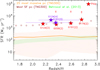 |
Fig. 20. Total SFR as a function of redshift of the PHz fields with multiple CO-detected sources at the same redshift (red full stars), and at all redshifts (purple full stars) compared with the total SFRs of simulated protoclusters. Horizontal bars represent the range of redshifts of all sources considered for the computation of the total SFR (see number in parenthesis). The PHz field names are annotated. The total SFR derived from the Planck fluxes and assuming a dust temperature of 30 K are shown as red crosses (these are available only for the subset of fields that are in the official PHz list). The predictions from the empirical models of Behroozi et al. (2013) are shown as green hatched region, those from the protocluster that would become the 25 most massive z = 0 clusters in the TNG300 simulation as salmon hatched area, the median SFR of the five most massive TNG300 simulated clusters as salmon thick line (adapted from Lim et al. 2021), and the most star-forming protocluster at 1.3 ≤ z ≤ 3 from the TNG300 simulations as brown open diamonds (Gouin et al. 2022; Nelson et al. 2019). |
Compared to the SFRs derived from Planck (Planck Collaboration XXXIX 2016), shown as red crosses in Fig. 20, our estimates are about 8−17 times lower, even when considering the CO-detected sources at different redshifts. This discrepancy has been solved in at least one field (G237; Polletta et al. 2021), where a detailed comparison between Planck and Herschel fluxes integrated over the same area has been carried out using deep Herschel observations from the HerMES survey (Oliver et al. 2012). The higher Planck SFRs are due to the large number of submm sources within the Planck beam (FWHM = 4.6 arcmin at 350 μm), typically ≳10 Herschel-detected sources, but most of them are along the line of sight of the protocluster and fainter than the IRAM 30-m telescope can detect (see Sect. 2.2 and Fig. 4).
6. Summary and conclusions
We report on IRAM 30-m/EMIR observations of 38 Herschel sources chosen as the brightest red submm sources in 18 Planck-selected (PHz) fields. These fields are considered protocluster candidates at z ≃ 2 − 4 hosting overdensities of DSFGs. We detected 40 CO lines on a total of 24 bright (S350 μm > 40 mJy) Herschel sources in 14 PHz fields. For the sources with no CO detection, we could not place any constraints on their redshift or CO luminosity, since the observations cover a limited frequency range (typically 16 GHz in bandwidth) and the exposure times were often too short for their brightness. For the 24 CO-detected sources, we estimated the SFRs and dust temperatures from fitting the submm spectral energy distribution (SED) with a modified blackbody. We also measured the CO lines’ intensity, luminosity, width, and (in ten cases) the CO SLED. We then derived the molecular gas masses, depletion times, and star formation efficiencies. We classified the sources as normal SFGs, or starbursts based on their position with respect to the  relation (Sargent et al. 2014).
The PHz-IRAM sample is characterized by the following average properties, ⟨zCO⟩ = 2.25 ± 0.09, ⟨SFR⟩ = 1043 ± 157 M⊙ yr−1, ⟨Tdust⟩ = 29.2 ± 0.9 K, ⟨FWHM⟩ = (317 ± 133) km s−1, ⟨Mgas⟩ = (4.0 ± 0.7) × 1011 M⊙, and ⟨τdep⟩ = 0.47 ± 0.07 Gyr. We compared the distributions of these quantities with those of cluster and protocluster members drawn from the literature with similar IR luminosities, and redshifts (1.4 ≤ z ≤ 3.1) and with the scaling relations describing normal SFGs, and starbursts at z ∼ 2.
Our main results are as follows:
-
The majority (80%) of the PHz-IRAM sources are consistent with the
 relation typical of normal SFGs; however, they are characterized, respectively, by SFRs and gas masses that are eight and five times, on average, higher than those typical of normal SFGs at similar redshifts. This result is not simply due to a selection effect that favors bright submm sources, as we observed a wide range of CO luminosities at fixed IR luminosity.
 -
We found evidence of multiplicity in three out of 24 (12 ± 7%) PHz-IRAM sources through the detection of two CO lines at inconsistent redshifts in one case and of double peak line profiles in other two cases. This percentage is consistent with those found in previous studies of bright SPIRE sources (9−23%; Montaña et al. 2021; Scudder et al. 2016). However, the derived properties suggest that multiplicity might affect a larger number of sources than our IRAM 30-m observations are able to reveal.
-
We found two or three Herschel sources in projected proximity at similar redshifts in four of the PHz fields where multiple Herschel sources were observed, supporting the idea that the PHz fields contain protoclusters at z ≃ 2 − 3. However, we also detect sources situated along the line of sight that contribute to the measured Planck flux, as predicted by Miller et al. (2015), and Negrello et al. (2017).
-
The CO SLED of eight out of ten PHz-IRAM sources with multiple CO transitions peaks at a low rotational number (Jup = 3), implying that a significant portion of the molecular gas must be at low densities, cold, and at low-excitation.
-
The CO line widths of the PHz-IRAM sample are, on average, smaller than typically observed in field SMGs as well as the cluster and protocluster sources from the literature. This difference is explained by an extended gas distribution to which the IRAM 30-m telescope is particularly sensitive.
-
About 20% of the PHz-IRAM sample is undergoing a starburst phase. Based on this result, we infer that these galaxies spend most of their lifetime as normal SFGs and exhibit a starburst phase only during 20% of their lifetime.
-
Compared to other protocluster members from the literature selected above a similar LIR limit, and across a similar redshift range (1.4 < z < 3.1), we find that our sources are characterized, on average, by slightly larger SFRs, and gas masses, but consistent SFEs, gas depletion timescales, and excitations.
-
We compared the SFRs of our PHz-IRAM sources with those predicted by state-of-the-art simulations for the most massive and most star-forming protoclusters (Nelson et al. 2019; Behroozi et al. 2013; Gouin et al. 2022). Although our total SFRs are consistent with the simulated ones, there is a significant discrepancy in terms of number of sources contributing to the total SFR, typically between 2 and 3 in our fields and 25 in the simulated protoclusters; this is also seen in the typical SFR of the galaxy members, with the observed ones being about ten times larger than in the simulations.
Overall the Planck-Herschel-IRAM selection reveals a class of SFGs that follows the scaling relations typical of normal SFGs at z ∼ 2, but with larger SFRs, and molecular gas masses than typically found in these galaxies. The peculiarity of our sources resides in their relatively low dust temperatures, low CO excitations, and relatively narrow CO line widths. These properties suggest that the majority of our sources are powered by a secular steady-state mechanism, and not by merger events. Multiplicity and some level of magnification due to gravitational lensing might also play a role in producing the observed properties.
Millimeter and CO observations at high spatial resolution would be necessary to assess whether the submm and CO fluxes are affected by multiplicity or gravitational lensing, and to determine whether the molecular gas is associated with a merger, a large massive disk, or extended emission. Such observations can also provide dynamical masses from the CO gas kinematics and morphology and, thus, the halo masses and baryonic fractions. These estimates are fundamental to devise improved characterizations of the environments of these galaxies. Finally, they are instrumental in identifying the optical-NIR counterparts to the submm emission and, thus, to obtain an accurate determination of the stellar mass by modeling the optical-NIR SED and of the SFR (by deblending the SPIRE flux as done in Kneissl et al. 2019).
The EMIR observational campaign, with a detection rate of ∼78% (14 PHz fields with a redshift estimate out of 18) was successful in providing an initial redshift guess for the overdensities in the PHz fields. Such information is crucial for an effective follow-up campaign at shorter wavelengths. Spectroscopic measurements through CO lines in the mm and in the rest-frame optical range are both necessary to fully study these structures as they typically reveal different galaxy types. The former are indeed more sensitive to heavily obscured galaxies that are often out of reach in the optical rest-frame, while the latter can reveal SFGs that are difficult to detect at mm wavelengths because they are not sufficiently massive in dust and molecular gas. Combining the results from these two wavelength windows is essential but not straightforward. With sensitive facilities such as ALMA, JWST, and future NIR spectrographs, these complementary datasets will become quickly accessible to many galaxy members, enabling the study of the stellar component as well as of both the ionized and molecular gas at similar angular resolution. Such a step forward in observational studies is essential for testing the simulations and improving our theoretical understanding on structure assembly and galaxy evolution.
A SPIRE source is defined red if detected in all three SPIRE bands and has flux density ratios S500/S350 > 0.6 and S350/S250 > 0.7 (see Planck Collaboration XXVII 2015).
Planck (http://www.esa.int/Planck) is a project of the European Space Agency (ESA) with instruments provided by two scientific consortia funded by ESA member states (in particular the lead countries France and Italy), with contributions from NASA (USA), and telescope reflectors provided by a collaboration between ESA and a scientific consortium led and funded by Denmark.
The PHz catalog is available at https://archives.esac.esa.int/doi/html/data/astronomy/planck/Catalogue_PHZ.html.
The RX map is obtained after subtracting from the map at 550 μm the image obtained by linearly interpolating the signal in the 350 μm, and 850 μm maps.
The Planck maps cleaning procedure consists in removing emission from the cosmic microwave background and foreground Galactic emission.
Herschel is an ESA space observatory with science instruments provided by European-led Principal Investigator consortia and with important participation from NASA.
The density contrast is defined as δPHz = (ρmax − ρbck)/ρbck.
The overdensity significance is defined as (ρmax − ρbck)/ρrms.
The FWHM of the Herschel-SPIRE beams are 18″ at 250 μm, 25″ at 350 μm, and 36″ at 500 μm.
S/N = SCO/rmsline, and rmsline = rms , where rmsch is the spectrum rms noise in mJy, and Δvch the spectral channel width in km s−1. Δvch ranges from 24 km s−1 to 91 km s−1, and is 37 ± 11 km s−1, on average.
Bothwell et al. (2013) report the following brightness temperature ratio values, rJ, J − 1 =  /
/ = 0.84, 0.52, 0.41, and 0.32 for J = 2, 3, 4, and 5, respectively.
Sargent et al. (2014) find log( /(K km s−1 pc2)) = 0.54 ± 0.02 + (0.81 ± 0.03) × log(LIR/L⊙) for normal SFGs.
The mean  , and IR luminosities of the SFGs in the PHz-IRAM sample, of the SFG protocluster members drawn from the literature, and of the normal SFGs at z = 1.4−2.4 are, respectively, ⟨log(
 /(K km s−1 pc2))⟩ = 11.0 ± 0.1, 10.7 ± 0.1, and 10.3 ± 0.1, and ⟨log(LIR/L⊙)⟩ = 12.9 ± 0.1, 12.6 ± 0.1, and 12.0 ± 0.1.
The median line widths and luminosities of the PHz-IRAM sources are median(FWHM) = 305 km s−1, and median (
 ) = (10.1
 K km s−1 pc2, for the protocluster members from the literature median(FWHM) = 490
 km s−1, and median(
 ) = (3.7
 K km s−1 pc2, and for the lensed SFGs median(FWHM) = 326
 km s−1, and median(
 ) = (36
 K km s−1 pc2.
See Remus, R.-S.’s presentation at the Galaxy Cluster Formation II (GCF 2021) – https://www.youtube.com/watch?v=iDVtDaElSLc.
According to Narayanan et al. (2012), the CO conversion factor can be expressed as min(6.3,10.7×W )/(Z/Z⊙
)0.65 where WCO is the CO surface brightness for a uniformly distributed molecular gas luminosity in units of (K km s−1), and Z/Z⊙
is the stellar metallicity in solar units.
)/(Z/Z⊙
)0.65 where WCO is the CO surface brightness for a uniformly distributed molecular gas luminosity in units of (K km s−1), and Z/Z⊙
is the stellar metallicity in solar units.
Acknowledgments
We kindly thank the second referee for a careful reading and for many suggestions that improved the clarity of the paper, and for replying in due time after the long-sought report from the first referee. We are very grateful to the IRAM staff for supporting us during the observations, for their warm hospitality, and for providing the data in the archive. We thank C. Gouin for providing the data on the most star-forming simulated IllustrisTNG300 protoclusters prior publication. We thank C. Gouin, N. Aghanim, and B. Garilli for useful discussions, and C. Casey for making the cmcirsed package available and for clarifying its usage. We thank T. Perdereau for his assistance during an observing run at IRAM 30-m. MP thanks the IRAP Institute for providing support and hospitality during her frequent visits. BLF gratefully acknowledges support from the Université de Paris-Saclay. This work is based on observations carried out under project numbers 107–14, 219–14, 197–15, 077–16, 186–16, 171–17, 085–19, 213–19, 178–20, and 082–21 with the IRAM 30-m telescope. IRAM is supported by INSU/CNRS (France), MPG (Germany) and IGN (Spain). The research leading to these results has received funding from the European Union’s Horizon 2020 research and innovation program under grant agreement No 730562 [RadioNet]. The work is based on observations obtained with Planckhttp://www.esa.int/Planck, an ESA science mission with instruments and contributions directly funded by ESA Member States, NASA, and Canada. This research has made use of data from HerMES project (https://hedam.lam.fr/HerMES/). HerMES is a Herschel Key Programme utilising Guaranteed Time from the SPIRE instrument team, ESAC scientists and a mission scientist. The HerMES data was accessed through the Herschel Database in Marseille (HeDaM – http://hedam.lam.fr) operated by CeSAM and hosted by the Laboratoire d’Astrophysique de Marseille. Software: This research made use of astropy, a community developed core Python package for astronomy (Astropy Collaboration 2018), of APLpy, an open-source plotting package for Python (Robitaille & Bressert 2012), of topcat (Taylor 2005), and of the HEALPix software (Górski et al. 2005).
References
- Amorín, R., Muñoz-Tuñón, C., Aguerri, J. A. L., & Planesas, P. 2016, A&A, 588, A23 [NASA ADS] [CrossRef] [EDP Sciences] [Google Scholar]
- Aravena, M., Carilli, C. L., Salvato, M., et al. 2012, MNRAS, 426, 258 [NASA ADS] [CrossRef] [Google Scholar]
- Aravena, M., Spilker, J. S., Bethermin, M., et al. 2016, MNRAS, 457, 4406 [Google Scholar]
- Astropy Collaboration (Price-Whelan, A. M., et al.) 2018, AJ, 156, 123 [Google Scholar]
- Behroozi, P. S., Marchesini, D., Wechsler, R. H., et al. 2013, ApJ, 777, L10 [Google Scholar]
- Béthermin, M., Daddi, E., Magdis, G., et al. 2015, A&A, 573, A113 [Google Scholar]
- Blain, A. W., Chapman, S. C., Smail, I., & Ivison, R. 2004, ApJ, 611, 725 [NASA ADS] [CrossRef] [Google Scholar]
- Bolatto, A. D., Wolfire, M., & Leroy, A. K. 2013, ARA&A, 51, 207 [CrossRef] [Google Scholar]
- Bothwell, M. S., Chapman, S. C., Tacconi, L., et al. 2010, MNRAS, 405, 219 [NASA ADS] [Google Scholar]
- Bothwell, M. S., Smail, I., Chapman, S. C., et al. 2013, MNRAS, 429, 3047 [Google Scholar]
- Cañameras, R., Nesvadba, N. P. H., Guery, D., et al. 2015, A&A, 581, A105 [Google Scholar]
- Cañameras, R., Yang, C., Nesvadba, N. P. H., et al. 2018, A&A, 620, A61 [Google Scholar]
- Calistro Rivera, G., Hodge, J. A., Smail, I., et al. 2018, ApJ, 863, 56 [Google Scholar]
- Calvi, R., Dannerbauer, H., Arrabal Haro, P., et al. 2021, MNRAS, 502, 4558 [NASA ADS] [CrossRef] [Google Scholar]
- Carilli, C. L., & Walter, F. 2013, ARA&A, 51, 105 [NASA ADS] [CrossRef] [Google Scholar]
- Carter, M., Lazareff, B., Maier, D., et al. 2012, A&A, 538, A89 [NASA ADS] [CrossRef] [EDP Sciences] [Google Scholar]
- Casasola, V., Magrini, L., Combes, F., et al. 2013, A&A, 558, A60 [NASA ADS] [CrossRef] [EDP Sciences] [Google Scholar]
- Casey, C. M. 2012, MNRAS, 425, 3094 [Google Scholar]
- Casey, C. M. 2016, ApJ, 824, 36 [CrossRef] [Google Scholar]
- Casey, C. M., Chapman, S. C., Neri, R., et al. 2011, MNRAS, 415, 2723 [NASA ADS] [CrossRef] [Google Scholar]
- Casey, C. M., Narayanan, D., & Cooray, A. 2014, Phys. Rep., 541, 45 [Google Scholar]
- Casey, C. M., Cooray, A., Capak, P., et al. 2015, ApJ, 808, L33 [NASA ADS] [CrossRef] [Google Scholar]
- Castignani, G., Jablonka, P., Combes, F., et al. 2020, A&A, 640, A64 [EDP Sciences] [Google Scholar]
- Chabrier, G. 2003, PASP, 115, 763 [Google Scholar]
- Champagne, J. B., Casey, C. M., Zavala, J. A., et al. 2021, ApJ, 913, 110 [NASA ADS] [CrossRef] [Google Scholar]
- Chapman, S. C., Helou, G., Lewis, G. F., & Dale, D. A. 2003, ApJ, 588, 186 [NASA ADS] [CrossRef] [Google Scholar]
- Chapman, S. C., Blain, A. W., Smail, I., & Ivison, R. J. 2005, ApJ, 622, 772 [NASA ADS] [CrossRef] [Google Scholar]
- Chapman, S. C., Blain, A., Ibata, R., et al. 2009, ApJ, 691, 560 [NASA ADS] [CrossRef] [Google Scholar]
- Chapman, S. C., Bertoldi, F., Smail, I., et al. 2015, MNRAS, 449, L68 [Google Scholar]
- Cicone, C., Mainieri, V., Circosta, C., et al. 2021, A&A, 654, L8 [NASA ADS] [CrossRef] [EDP Sciences] [Google Scholar]
- Clements, D. L., Braglia, F. G., Hyde, A. K., et al. 2014, MNRAS, 439, 1193 [NASA ADS] [CrossRef] [Google Scholar]
- Clements, D. L., Pearson, C., Farrah, D., et al. 2018, MNRAS, 475, 2097 [NASA ADS] [CrossRef] [Google Scholar]
- Coogan, R. T., Daddi, E., Sargent, M. T., et al. 2018, MNRAS, 479, 703 [NASA ADS] [Google Scholar]
- Cortese, L., Fritz, J., Bianchi, S., et al. 2014, MNRAS, 440, 942 [Google Scholar]
- Daddi, E., Bournaud, F., Walter, F., et al. 2010, ApJ, 713, 686 [NASA ADS] [CrossRef] [Google Scholar]
- Daddi, E., Dannerbauer, H., Liu, D., et al. 2015, A&A, 577, A46 [NASA ADS] [CrossRef] [EDP Sciences] [Google Scholar]
- D’Amato, Q., Gilli, R., Prandoni, I., et al. 2020, A&A, 641, L6 [NASA ADS] [CrossRef] [EDP Sciences] [Google Scholar]
- Dannerbauer, H., Lehnert, M. D., Emonts, B., et al. 2017, A&A, 608, A48 [NASA ADS] [CrossRef] [EDP Sciences] [Google Scholar]
- Dekel, A., & Birnboim, Y. 2006, MNRAS, 368, 2 [NASA ADS] [CrossRef] [Google Scholar]
- Dessauges-Zavadsky, M., Zamojski, M., Schaerer, D., et al. 2015, A&A, 577, A50 [NASA ADS] [CrossRef] [EDP Sciences] [Google Scholar]
- Eisenhardt, P. R. M., Brodwin, M., Gonzalez, A. H., et al. 2008, ApJ, 684, 905 [Google Scholar]
- Emonts, B. H. C., Lehnert, M. D., Villar-Martín, M., et al. 2016, Science, 354, 1128 [NASA ADS] [CrossRef] [Google Scholar]
- Emonts, B. H. C., Cai, Z., Prochaska, J. X., Li, Q., & Lehnert, M. D. 2019, ApJ, 887, 86 [NASA ADS] [CrossRef] [Google Scholar]
- Erb, D. K., Steidel, C. C., Shapley, A. E., et al. 2006a, ApJ, 646, 107 [NASA ADS] [CrossRef] [Google Scholar]
- Erb, D. K., Shapley, A. E., Pettini, M., et al. 2006b, ApJ, 644, 813 [NASA ADS] [CrossRef] [Google Scholar]
- Fixsen, D. J., Bennett, C. L., & Mather, J. C. 1999, ApJ, 526, 207 [Google Scholar]
- Flores-Cacho, I., Pierini, D., Soucail, G., et al. 2016, A&A, 585, A54 [NASA ADS] [CrossRef] [EDP Sciences] [Google Scholar]
- Foltz, R., Wilson, G., Muzzin, A., et al. 2018, ApJ, 866, 136 [NASA ADS] [CrossRef] [Google Scholar]
- Genzel, R., Tacconi, L. J., Combes, F., et al. 2012, ApJ, 746, 69 [Google Scholar]
- Gildas Team 2013, Astrophysics Source Code Library [record ascl:1305.010] [Google Scholar]
- Ginolfi, M., Maiolino, R., Nagao, T., et al. 2017, MNRAS, 468, 3468 [CrossRef] [Google Scholar]
- Gobat, R., Daddi, E., Onodera, M., et al. 2011, A&A, 526, A133 [NASA ADS] [CrossRef] [EDP Sciences] [Google Scholar]
- Gómez-Guijarro, C., Riechers, D. A., Pavesi, R., et al. 2019, ApJ, 872, 117 [CrossRef] [Google Scholar]
- Górski, K. M., Hivon, E., Banday, A. J., et al. 2005, ApJ, 622, 759 [Google Scholar]
- Goto, T., Takagi, T., Matsuhara, H., et al. 2010, A&A, 514, A6 [NASA ADS] [CrossRef] [EDP Sciences] [Google Scholar]
- Gouin, C., Aghanim, N., Dole, H., Polletta, M., & Park, C. 2022, A&A, submitted [arXiv:2203.16276] [NASA ADS] [CrossRef] [EDP Sciences] [Google Scholar]
- Granato, G. L., Ragone-Figueroa, C., Domínguez-Tenreiro, R., et al. 2015, MNRAS, 450, 1320 [NASA ADS] [CrossRef] [Google Scholar]
- Griffin, M. J., Abergel, A., Abreu, A., et al. 2010, A&A, 518, L3 [EDP Sciences] [Google Scholar]
- Harrington, K. C., Yun, M. S., Magnelli, B., et al. 2018, MNRAS, 474, 3866 [Google Scholar]
- Harris, A. I., Baker, A. J., Frayer, D. T., et al. 2012, ApJ, 752, 152 [NASA ADS] [CrossRef] [Google Scholar]
- Hatch, N. A., Kurk, J. D., Pentericci, L., et al. 2011, MNRAS, 415, 2993 [NASA ADS] [CrossRef] [Google Scholar]
- Hayashi, M., Kodama, T., Kohno, K., et al. 2017, ApJ, 841, L21 [NASA ADS] [CrossRef] [Google Scholar]
- Hezaveh, Y. D., Marrone, D. P., & Holder, G. P. 2012, ApJ, 761, 20 [NASA ADS] [CrossRef] [Google Scholar]
- Hodge, J. A., Carilli, C. L., Walter, F., et al. 2012, ApJ, 760, 11 [Google Scholar]
- Huang, J. S., Rigopoulou, D., Magdis, G., et al. 2014, ApJ, 784, 52 [Google Scholar]
- Hung, C.-L., Casey, C. M., Chiang, Y.-K., et al. 2016, ApJ, 826, 130 [NASA ADS] [CrossRef] [Google Scholar]
- Inoue, S., Takagi, T., Miyazaki, A., et al. 2021, MNRAS, 506, 84 [NASA ADS] [CrossRef] [Google Scholar]
- Ivison, R. J., Papadopoulos, P. P., Smail, I., et al. 2011, MNRAS, 412, 1913 [Google Scholar]
- Ivison, R. J., Smail, I., Amblard, A., et al. 2012, MNRAS, 425, 1320 [NASA ADS] [CrossRef] [Google Scholar]
- Ivison, R. J., Swinbank, A. M., Smail, I., et al. 2013, ApJ, 772, 137 [NASA ADS] [CrossRef] [Google Scholar]
- Ivison, R. J., Biggs, A. D., Bremer, M., Arumugam, V., & Dunne, L. 2020, MNRAS, 496, 4358 [NASA ADS] [CrossRef] [Google Scholar]
- Jin, S., Dannerbauer, H., Emonts, B., et al. 2021, A&A, 652, A11 [NASA ADS] [CrossRef] [EDP Sciences] [Google Scholar]
- Jones, L. H., Rosenthal, M. J., Barger, A. J., & Cowie, L. L. 2021, ApJ, 916, 46 [NASA ADS] [CrossRef] [Google Scholar]
- Kato, Y., Matsuda, Y., Smail, I., et al. 2016, MNRAS, 460, 3861 [Google Scholar]
- Keating, L. C., Richings, A. J., Murray, N., et al. 2020, MNRAS, 499, 837 [NASA ADS] [CrossRef] [Google Scholar]
- Kennicutt, R. C., Jr. 1998, ARA&A, 36, 189 [Google Scholar]
- Kereš, D., Katz, N., Weinberg, D. H., & Davé, R. 2005, MNRAS, 363, 2 [Google Scholar]
- Kneissl, R., Polletta, M., Martinache, C., et al. 2019, A&A, 625, A96 [NASA ADS] [CrossRef] [EDP Sciences] [Google Scholar]
- Koyama, Y., Polletta, M. D. C., Tanaka, I., et al. 2021, MNRAS, 503, L1 [NASA ADS] [CrossRef] [Google Scholar]
- Lacaille, K. M., Chapman, S. C., Smail, I., et al. 2019, MNRAS, 488, 1790 [NASA ADS] [CrossRef] [Google Scholar]
- Lee, M. M., Tanaka, I., Kawabe, R., et al. 2017, ApJ, 842, 55 [CrossRef] [Google Scholar]
- Lee, M. M., Tanaka, I., Kawabe, R., et al. 2019, ApJ, 883, 92 [NASA ADS] [CrossRef] [Google Scholar]
- Li, Q., Wang, R., Dannerbauer, H., et al. 2021, ApJ, 922, 236 [NASA ADS] [CrossRef] [Google Scholar]
- Lim, S., Scott, D., Babul, A., et al. 2021, MNRAS, 501, 1803 [Google Scholar]
- López-Sanjuan, C., Le Fèvre, O., Tasca, L. A. M., et al. 2013, A&A, 553, A78 [NASA ADS] [CrossRef] [EDP Sciences] [Google Scholar]
- MacKenzie, T. P., Scott, D., Bianconi, M., et al. 2017, MNRAS, 468, 4006 [NASA ADS] [CrossRef] [Google Scholar]
- Magdis, G. E., Elbaz, D., Hwang, H. S., et al. 2010, MNRAS, 409, 22 [NASA ADS] [CrossRef] [Google Scholar]
- Magdis, G. E., Daddi, E., Béthermin, M., et al. 2012, ApJ, 760, 6 [NASA ADS] [CrossRef] [Google Scholar]
- Magdis, G. E., Rigopoulou, D., Daddi, E., et al. 2017, A&A, 603, A93 [NASA ADS] [CrossRef] [EDP Sciences] [Google Scholar]
- Magnelli, B., Popesso, P., Berta, S., et al. 2013, A&A, 553, A132 [NASA ADS] [CrossRef] [EDP Sciences] [Google Scholar]
- Magnelli, B., Lutz, D., Saintonge, A., et al. 2014, A&A, 561, A86 [NASA ADS] [CrossRef] [EDP Sciences] [Google Scholar]
- Magnelli, B., Karim, A., Staguhn, J., et al. 2019, ApJ, 877, 45 [NASA ADS] [CrossRef] [Google Scholar]
- Martinache, C., Rettura, A., Dole, H., et al. 2018, A&A, 620, A198 [NASA ADS] [CrossRef] [EDP Sciences] [Google Scholar]
- Miller, T. B., Hayward, C. C., Chapman, S. C., & Behroozi, P. S. 2015, MNRAS, 452, 878 [NASA ADS] [CrossRef] [Google Scholar]
- Miller, T. B., Chapman, S. C., Aravena, M., et al. 2018, Nature, 556, 469 [CrossRef] [Google Scholar]
- Montaña, A., Zavala, J. A., Aretxaga, I., et al. 2021, MNRAS, 505, 5260 [CrossRef] [Google Scholar]
- Muldrew, S. I., Hatch, N. A., & Cooke, E. A. 2015, MNRAS, 452, 2528 [NASA ADS] [CrossRef] [Google Scholar]
- Narayanan, D., & Krumholz, M. R. 2014, MNRAS, 442, 1411 [NASA ADS] [CrossRef] [Google Scholar]
- Narayanan, D., Krumholz, M. R., Ostriker, E. C., & Hernquist, L. 2012, MNRAS, 421, 3127 [NASA ADS] [CrossRef] [Google Scholar]
- Narayanan, D., Turk, M., Feldmann, R., et al. 2015, Nature, 525, 496 [NASA ADS] [CrossRef] [Google Scholar]
- Negrello, M., Gonzalez-Nuevo, J., De Zotti, G., et al. 2017, MNRAS, 470, 2253 [NASA ADS] [CrossRef] [Google Scholar]
- Nelson, D., Springel, V., Pillepich, A., et al. 2019, Comput. Astrophys. Cosmol., 6, 2 [Google Scholar]
- Newman, A. B., Ellis, R. S., Andreon, S., et al. 2014, ApJ, 788, 51 [NASA ADS] [CrossRef] [Google Scholar]
- Noble, A. G., McDonald, M., Muzzin, A., et al. 2017, ApJ, 842, L21 [Google Scholar]
- Noble, A. G., Muzzin, A., McDonald, M., et al. 2019, ApJ, 870, 56 [Google Scholar]
- Oliver, S. J., Bock, J., Altieri, B., et al. 2012, MNRAS, 424, 1614 [NASA ADS] [CrossRef] [Google Scholar]
- Oteo, I., Ivison, R. J., Dunne, L., et al. 2018, ApJ, 856, 72 [Google Scholar]
- Overzier, R. A. 2016, A&ARv, 24, 14 [Google Scholar]
- Pallero, D., Gómez, F. A., Padilla, N. D., et al. 2019, MNRAS, 488, 847 [NASA ADS] [CrossRef] [Google Scholar]
- Papadopoulos, P. P., Isaak, K., & van der Werf, P. 2010, ApJ, 711, 757 [Google Scholar]
- Papadopoulos, P. P., van der Werf, P. P., Xilouris, E. M., et al. 2012, MNRAS, 426, 2601 [NASA ADS] [CrossRef] [Google Scholar]
- Pilbratt, G. L., Riedinger, J. R., Passvogel, T., et al. 2010, A&A, 518, L1 [NASA ADS] [CrossRef] [EDP Sciences] [Google Scholar]
- Planck Collaboration XXVII. 2015, A&A, 582, A30 [NASA ADS] [CrossRef] [EDP Sciences] [Google Scholar]
- Planck Collaboration XXVI. 2016, A&A, 594, A26 [NASA ADS] [CrossRef] [EDP Sciences] [Google Scholar]
- Planck Collaboration XXXIX. 2016, A&A, 596, A100 [NASA ADS] [CrossRef] [EDP Sciences] [Google Scholar]
- Planck Collaboration VI. 2020, A&A, 641, A6 [NASA ADS] [CrossRef] [EDP Sciences] [Google Scholar]
- Pokhrel, R., Gutermuth, R., Ali, B., et al. 2016, MNRAS, 461, 22 [NASA ADS] [CrossRef] [Google Scholar]
- Polletta, M., Soucail, G., Dole, H., et al. 2021, A&A, 654, A121 [NASA ADS] [CrossRef] [EDP Sciences] [Google Scholar]
- Riechers, D. A. 2011, ApJ, 730, 108 [NASA ADS] [CrossRef] [Google Scholar]
- Robitaille, T., & Bressert, E. 2012, Astrophysics Source Code Library [record ascl:1208.017] [Google Scholar]
- Rodighiero, G., Daddi, E., Baronchelli, I., et al. 2011, ApJ, 739, L40 [Google Scholar]
- Romano, M., Cassata, P., Morselli, L., et al. 2021, A&A, 653, A111 [NASA ADS] [CrossRef] [EDP Sciences] [Google Scholar]
- Rotermund, K. M., Chapman, S. C., Phadke, K. A., et al. 2021, MNRAS, 502, 1797 [NASA ADS] [CrossRef] [Google Scholar]
- Rudnick, G., Hodge, J., Walter, F., et al. 2017, ApJ, 849, 27 [NASA ADS] [CrossRef] [Google Scholar]
- Saintonge, A., Lutz, D., Genzel, R., et al. 2013, ApJ, 778, 2 [Google Scholar]
- Sanders, D. B., & Mirabel, I. F. 1996, ARA&A, 34, 749 [Google Scholar]
- Sanders, D. B., Soifer, B. T., Elias, J. H., et al. 1988, ApJ, 325, 74 [Google Scholar]
- Sargent, M. T., Daddi, E., Béthermin, M., et al. 2014, ApJ, 793, 19 [NASA ADS] [CrossRef] [Google Scholar]
- Schirm, M. R. P., Wilson, C. D., Parkin, T. J., et al. 2014, ApJ, 781, 101 [Google Scholar]
- Scudder, J. M., Oliver, S., Hurley, P. D., et al. 2016, MNRAS, 460, 1119 [NASA ADS] [CrossRef] [Google Scholar]
- Sharon, C. E., Riechers, D. A., Hodge, J., et al. 2016, ApJ, 827, 18 [Google Scholar]
- Shimwell, T. W., Röttgering, H. J. A., Best, P. N., et al. 2017, A&A, 598, A104 [NASA ADS] [CrossRef] [EDP Sciences] [Google Scholar]
- Shimwell, T. W., Hardcastle, M. J., Tasse, C., et al. 2022, A&A, 659, A1 [NASA ADS] [CrossRef] [EDP Sciences] [Google Scholar]
- Solimano, M., González-López, J., Barrientos, L. F., et al. 2021, A&A, 655, A42 [CrossRef] [Google Scholar]
- Solomon, P. M., Downes, D., Radford, S. J. E., & Barrett, J. W. 1997, ApJ, 478, 144 [NASA ADS] [CrossRef] [Google Scholar]
- Speagle, J. S., Steinhardt, C. L., Capak, P. L., & Silverman, J. D. 2014, ApJS, 214, 15 [Google Scholar]
- Stach, S. M., Swinbank, A. M., Smail, I., et al. 2017, ApJ, 849, 154 [NASA ADS] [CrossRef] [Google Scholar]
- Strazzullo, V., Coogan, R. T., Daddi, E., et al. 2018, ApJ, 862, 64 [NASA ADS] [CrossRef] [Google Scholar]
- Symeonidis, M., & Page, M. J. 2018, MNRAS, 479, L91 [Google Scholar]
- Symeonidis, M., Vaccari, M., Berta, S., et al. 2013, MNRAS, 431, 2317 [Google Scholar]
- Tacconi, L. J., Genzel, R., Smail, I., et al. 2008, ApJ, 680, 246 [Google Scholar]
- Tacconi, L. J., Neri, R., Genzel, R., et al. 2013, ApJ, 768, 74 [NASA ADS] [CrossRef] [Google Scholar]
- Tadaki, K.-I., Kodama, T., Tamura, Y., et al. 2014, ApJ, 788, L23 [NASA ADS] [CrossRef] [Google Scholar]
- Tadaki, K.-I., Kodama, T., Hayashi, M., et al. 2019, PASJ, 71, 40 [NASA ADS] [CrossRef] [Google Scholar]
- Taniguchi, Y., & Shioya, Y. 1998, ApJ, 501, L167 [NASA ADS] [CrossRef] [Google Scholar]
- Taylor, M. B. 2005, in Astronomical Data Analysis Software and Systems XIV, eds. P. Shopbell, M. Britton, & R. Ebert, ASP Conf. Ser., 347, 29 [Google Scholar]
- Thomas, D., Maraston, C., Bender, R., & Mendes de Oliveira, C. 2005, ApJ, 621, 673 [Google Scholar]
- Umehata, H., Tamura, Y., Kohno, K., et al. 2015, ApJ, 815, L8 [Google Scholar]
- Umehata, H., Smail, I., Steidel, C. C., et al. 2021, ApJ, 918, 69 [NASA ADS] [CrossRef] [Google Scholar]
- Wagg, J., Pope, A., Alberts, S., et al. 2012, ApJ, 752, 91 [NASA ADS] [CrossRef] [Google Scholar]
- Walter, F., Carilli, C., Neeleman, M., et al. 2020, ApJ, 902, 111 [Google Scholar]
- Wang, T., Elbaz, D., Daddi, E., et al. 2016, ApJ, 828, 56 [NASA ADS] [CrossRef] [Google Scholar]
- Wang, T., Elbaz, D., Daddi, E., et al. 2018, ApJ, 867, L29 [NASA ADS] [CrossRef] [Google Scholar]
- Webb, T. M. A., Lowenthal, J., Yun, M., et al. 2017, ApJ, 844, L17 [CrossRef] [Google Scholar]
- Weiß, A., Downes, D., Neri, R., et al. 2007, A&A, 467, 955 [NASA ADS] [CrossRef] [EDP Sciences] [Google Scholar]
- Weiß, A., De Breuck, C., Marrone, D. P., et al. 2013, ApJ, 767, 88 [Google Scholar]
- Yang, C., Omont, A., Beelen, A., et al. 2017, A&A, 608, A144 [NASA ADS] [CrossRef] [EDP Sciences] [Google Scholar]
- Zhang, Z.-Y., Henkel, C., Gao, Y., et al. 2014, A&A, 568, A122 [NASA ADS] [CrossRef] [EDP Sciences] [Google Scholar]
- Zirm, A. W., Toft, S., & Tanaka, M. 2012, ApJ, 744, 181 [NASA ADS] [CrossRef] [Google Scholar]
Appendix A: Tables: IRAM observations
The list of observed targets, the log of the IRAM observations, and the instrument set-up are listed in Tables A.1, A.2, and A.3.
List of observed targets.
EMIR observations log.
EMIR frequency coverage and integration time.
Appendix B: EMIR spectra
In this section, we show the spectra of the detected CO lines listed in Table 2. In Fig. B.1, and B.2, we show the sources where multiple transitions have been detected, and in Fig. B.3 those with only one CO line detection. The CO line transition is annotated in the corresponding panel only in the case of multiple line detections per source.
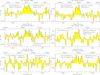 |
Fig. B.1. Emission line detections in the continuum-subtracted EMIR spectra of the PHz-IRAM sources where three CO transitions have been observed. The fit to each line is overlaid with a red curve for single Gaussian fits, or with a blue curve for double Gaussian fits. Source name, line transition and observed central frequency, intensity, and width are annotated in each panel. All the left panels refer to one source and all the right panels to the other. |
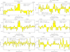 |
Fig. B.1. continued. |
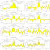 |
Fig. B.2. Emission line detections in the continum-subtracted EMIR spectra of the PHz-IRAM sources where two CO transitions have been detected. The fit to each line is overlaid with a red curve for single Gaussian fits, or with a blue curve for double Gaussian fits. Source name, line transition and observed central frequency, intensity, and width are annotated in each panel. Each row corresponds to a specific source. |
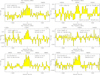 |
Fig. B.2. continued. |
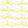 |
Fig. B.3. Emission line detections in the continum-subtracted EMIR spectra of the PHz-IRAM sources where a single CO line has been detected. The Gaussian fit to each line is overlaid with a red curve. Source name, line observed central frequency, intensity, and width are annotated in each panel. |
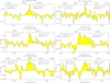 |
Fig. B.3. continued. |
Appendix C: Literature samples
In order to compare the properties of the PHz-IRAM sources with other CO-detected sources found in overdense regions, we compiled published datasets of cluster and protocluster galaxies at 1.4 < z < 3.1 that have been observed in CO, and for which a SFR or the total IR luminosity are available. We list the name of the protocluster to, their CO redshift, when available, as well as the line transition, intensity, and width in Table C.1. For the purposes of this work, we selected a subsample with IR luminosities above the LIR limit of the PHz-IRAM sample minus 0.2 dex, that is, log(LIR) > 11.44+0.5×z (see details in Sect. 4.4, and Fig. 10, and sources flagged with b in the Table). For the comparison, we converted the CO luminosities into  using the brightness temperature ratios from Bothwell et al. (2013), as done for the PHz-IRAM sample. In a few cases, the IR luminosity was derived from the SFR using the relation LIR/L⊙ = SFR/(9.5×10−11) with SFR in M⊙ yr−1, assuming a Chabrier (2003) IMF, even if the SFR was derived from other observables, such as the SED or the Hα luminosity.
List of protocluster and cluster galaxies from the literature.
Appendix D: Impact of the CO–H2 conversion factor
Using simulations, Narayanan et al. (2012) showed that the αCO conversion factor covers a wide range of values depending on several physical parameters and, in particular, the molecular gas surface brightness and the gas-phase metallicity17. Since we do not have measurements of CO surface brightness (WCO) nor of the gas-phase metallicity, we approximate the former as the  /area. We considered a compact and an extended area given by circular regions with radii of Rgas = 5, and 25 kpc, respectively. We assumed solar metallicity, even though galaxies at z∼2 and the members of one PHz protocluster for which stellar metallicities have been measured exhibit sub-solar metallicities (Erb et al. 2006b; Polletta et al. 2021). The predicted αCO values for our sources obtained assuming compact and extended molecular gas distributions as a function of CO surface brightness are shown in Fig. D.1. We also show the value of αCO = 3.5 M⊙ pc−2 (K km s−1)−1 adopted in this work. The predicted αCO values in the case of extended distribution range between 1.9 and 4.9, with a mean value of 3.3±0.1, close to the assumed value. Assuming a different αCO, within this range, would result in a gas mass a factor of 1.8 smaller or 1.4 larger, at the most. The αCO predicted by the relation that depends only on the metallicity (e.g., Genzel et al. 2012; Amorín et al. 2016) would be 4.8, assuming solar metallicity. This choice would yield gas masses, and depletion times systematically larger by a factor of 1.4.
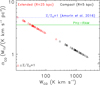 |
Fig. D.1. Predicted αCO conversion factors (open triangles) by the functional form derived in Narayanan et al. (2012) in the case of solar gas-phase metallicity and compact (radius of 5 kpc; red), or extended (radius of 25 kpc; black) molecular gas distributions, as a function of CO surface brightness given by the ratio between |

Lower metallicities would entail higher αCO values and unreasonably high gas masses. On the other hand, the inferred gas masses, under the assumption of a αCO = 3.5, agree with the scaling relations, suggesting that the metallicities of our sources might be already solar. This might be due to an observational bias since it is challenging to detect CO emission in galaxies with low metallicities. We conclude that the gas mass estimates might differ, at the most, by +0.15 dex, or −0.27 dex compared with those we derive assuming αCO = 3.5.
All Tables
All Figures
|
Fig. 1. Scheme representing the number of fields with one (green), two (light blue), four (orange), five (yellow), or nine (red) targets observed with IRAM 30-m. The area of each rectangle is proportional to the number of fields. |
| In the text | |
|
Fig. 2. SPIRE-350 μm flux density distribution of the targets observed with IRAM in this study (solid magenta line: CO-detected, and dashed turquoise line: CO not-detected), and of all SPIRE sources (black line) situated in the PHz fields in the region of the sky visible from the IRAM-30 m telescope site (δ ≳ −2°). |
| In the text | |
|
Fig. 3. SPIRE colors of the targets selected for IRAM observations (magenta full circles: CO-detected; turquoise full circles: IRAM observed but not CO-detected) and of all SPIRE sources (black circles) situated in the PHz fields in the region of the sky visible from the IRAM-30 m telescope site (δ ≥ −2°). The red lines enclose the region of red SPIRE colors. Top and right panels: submm color distributions normalized at the peak (gray: all PHz-SPIRE sources at δ ≥ −2; magenta: CO detected; cyan: CO not-detected). |
| In the text | |
|
Fig. 4. 15′×15′ Herschel RGB (red: 500 μm, green: 350 μm, blue: 250 μm) maps centered on the IRAM observed PHz fields presented here. SPIRE sources are indicated with open circles (red: red submm colors; blue: blue submm colors; yellow: not detected in all three bands, thus preventing a color classification). IRAM targets are indicated with big stars (red: CO detection at similar redshift (i.e., Δz/(1 + z) < 0.02), cyan: CO detected, there is only one detection or multiple detections at different redshifts (i.e., Δz/(1 + z) > 0.02); white: CO not detected). Yellow contours represent the Planck red-excess emission (50%, 70%, and 90% of the maximum value). Green contours represent the overdensity significance of red SPIRE sources (starting at 3σ, with steps of 1σ). (a) G176. (b) G223. (c) G173. (d) G162. (e) G006. (f) G237. (g) G191. (h) G088. (i) G059. |
| In the text | |
|
Fig. 4. continued. (a) G073. (b) G124. (c) G072. (d) G112. (e) G143. (f) G131. (g) G052. (h) G068. (i) G063. |
| In the text | |
|
Fig. 5. EMIR integration time per frequency band of all observations. Boxes are shown in case some scans were not used in specific sub-bands. Observations relative to the same target are connected with dotted lines. The observations that yielded at least one CO line detection are shown in magenta, and those with no detections are shown in turquoise. |
| In the text | |
|
Fig. 6. EMIR integration time of all observations per source (full circle connected by a straight line) as a function of the source flux density at 350 μm. The source ID is noted. The observations that yielded at least one CO line detection are shown in magenta and those with no detections are shown in turquoise. |
| In the text | |
|
Fig. 7. Peak flux of the detected CO lines (full orange circles if S/N > 4.0, and purple if S/N ≤ 4.0) as a function of the integration time. The line rms is also shown (black triangles) and connected to the corresponding measured flux by a dotted vertical line. The expected trend of rmsline with the integration time is shown as dashed green line and the detection threshold of 4 × rmsline as dotted green line. The rmsline varies with channel width and depends on the line width. |
| In the text | |
|
Fig. 8. Peak flux of the detected CO lines (full orange circles if S/N > 4.0, and purple if S/N ≤ 4.0) as a function of flux density at 350 μm. |
| In the text | |
|
Fig. 9. Redshift distribution derived from secure (red) and dubious (blue) CO line identifications of 24 PHz sources. The dashed vertical black line represents the mean redshift, ⟨zCO⟩ = 2.25 ± 0.09, obtained from the secure identifications. |
| In the text | |
|
Fig. 10. Total IR (8−1000 μm) luminosity or SFR as a function of redshift for the PHz-IRAM sources (full red stars for secure line identifications and full blue stars for uncertain line identifications) and for 1.4 < z < 3.1 cluster and protocluster members from the literature (gray triangles and crosses). In the case of multiple EMIR detections associated with the same SPIRE source, an upper limit to LIR was reported with a downward pointing arrow. Blue stars connected with a solid blue line refer to the same source and to two possible redshifts. The black dashed line represents the total IR luminosity of a source with S(350 μm) = 40 mJy and Tdust = 30 K (derived using the cmcirsed package; Casey 2012) corresponding to the selection of the majority of the PHz-IRAM targets. The dotted line is the same LIR limit scaled by −0.2 dex and used to select a subset of cluster and protocluster members from the literature for comparison (gray triangles). |
| In the text | |
|
Fig. 11. Main panel: dust temperature as a function of the IR (8−1000 μm) luminosity for the PHz-IRAM sources (full stars, red for secure CO line identifications, and blue for the uncertain ones). The shaded orange area shows the local Tdust − LIR relation derived by Chapman et al. (2003), linearly extrapolated to 1013 L⊙. The shaded cyan area shows the range of dust temperatures for main sequence galaxies in the redshift range of the PHz-IRAM sources (1.3 < z < 2.8) according to the relation found by Magnelli et al. (2014), and extended to LIR > 1013 L⊙. The shaded green area presents results for z ≃ 2 SMGs from Chapman et al. (2005). The purple diamonds represent the relation found for z < 1.5 SPIRE sources by Symeonidis et al. (2013). Top and right panels: distributions of SFR (and IR luminosity) and dust temperature, respectively, for all PHz-IRAM sources. |
| In the text | |
|
Fig. 12. CO SLEDs of the PHz-IRAM sources (full red circles connected by a black solid line). The CO SLEDs of different types of galaxies normalized to the observed CO(3−2) intensity of each PHz-IRAM source are shown for comparison in each panel as dotted lines: the Milky Way (purple; Fixsen et al. 1999); SMGs (orange), QSO (brown), the prototypical starburst galaxy M 82 (green), and color-selected SFGs (CSG; blue) from Carilli & Walter (2013); and BzK galaxies at z ∼ 1.5 (cyan) from Daddi et al. (2015). The solid magenta line in each panel shows the SLED model from Narayanan & Krumholz (2014) obtained assuming the annotated SFR density in M⊙ yr−1 kpc−2. |
| In the text | |
|
Fig. 13. CO SLEDs of protocluster members from the literature (full pink circles connected by black lines; Coogan et al. 2018; Casey 2016; Lee et al. 2017, 2019; Gómez-Guijarro et al. 2019) compared with the CO SLED of different types or sources (dotted lines of color as in Fig. 12). Downward pointing arrows indicate upper limits. The protocluster and source names are annotated (see Table C.1). Source names between parentheses are those that do not satisfy the IR luminosity selection criterion. |
| In the text | |
|
Fig. 14. CO(1−0) luminosity as a function of redshift for the PHz-IRAM sources. Symbols are the same as in Fig. 10. The purple and magenta curves show the expected |
| In the text | |
|
Fig. 15. Total IR (8−1000 μm) luminosity or SFR as a function of CO(1−0) luminosity for the PHz-IRAM sources and for 1.4 < z < 3.1 cluster and protocluster members from the literature (same symbols as in Fig. 14). The protocluster massive spiral HAE229 (Dannerbauer et al. 2017) is shown as full gold triangle. The solid green line and the dashed magenta line represent, respectively, the average relations for normal SFGs and starburst galaxies (Sargent et al. 2014). Open magenta or green squares are overplotted over the PHz sources classified as starburst, or normal SFGs based on the agreement with the drawn relations. In the inset, we show the same graph and data, but extended to lower luminosities and include a sample of CO-detected normal SFGs at z = 1.4−2.4 (lilac open circles; Daddi et al. 2010; Tacconi et al. 2013). |
| In the text | |
|
Fig. 16. Star formation efficiency (SFE) of the PHz-IRAM sources as a function of gas mass. Symbols as in Fig. 15. |
| In the text | |
|
Fig. 17. Estimated depletion times of the PHz-IRAM sources as a function of redshift. Symbols as in Fig. 15. The turquoise region is the locus of normal SFGs (Saintonge et al. 2013). |
| In the text | |
|
Fig. 18. Estimated redshift by which the molecular gas would be depleted (zdep) assuming the current SFR and 100% conversion of gas into stars with no refueling (red solid line: sources with secure redshift, blue dashed line: sources with uncertain redshift). The vertical black dashed line represents the mean zdep value derived from the sources with secure redshifts. |
| In the text | |
|
Fig. 19.
|
| In the text | |
|
Fig. 20. Total SFR as a function of redshift of the PHz fields with multiple CO-detected sources at the same redshift (red full stars), and at all redshifts (purple full stars) compared with the total SFRs of simulated protoclusters. Horizontal bars represent the range of redshifts of all sources considered for the computation of the total SFR (see number in parenthesis). The PHz field names are annotated. The total SFR derived from the Planck fluxes and assuming a dust temperature of 30 K are shown as red crosses (these are available only for the subset of fields that are in the official PHz list). The predictions from the empirical models of Behroozi et al. (2013) are shown as green hatched region, those from the protocluster that would become the 25 most massive z = 0 clusters in the TNG300 simulation as salmon hatched area, the median SFR of the five most massive TNG300 simulated clusters as salmon thick line (adapted from Lim et al. 2021), and the most star-forming protocluster at 1.3 ≤ z ≤ 3 from the TNG300 simulations as brown open diamonds (Gouin et al. 2022; Nelson et al. 2019). |
| In the text | |
|
Fig. B.1. Emission line detections in the continuum-subtracted EMIR spectra of the PHz-IRAM sources where three CO transitions have been observed. The fit to each line is overlaid with a red curve for single Gaussian fits, or with a blue curve for double Gaussian fits. Source name, line transition and observed central frequency, intensity, and width are annotated in each panel. All the left panels refer to one source and all the right panels to the other. |
| In the text | |
|
Fig. B.1. continued. |
| In the text | |
|
Fig. B.2. Emission line detections in the continum-subtracted EMIR spectra of the PHz-IRAM sources where two CO transitions have been detected. The fit to each line is overlaid with a red curve for single Gaussian fits, or with a blue curve for double Gaussian fits. Source name, line transition and observed central frequency, intensity, and width are annotated in each panel. Each row corresponds to a specific source. |
| In the text | |
|
Fig. B.2. continued. |
| In the text | |
|
Fig. B.3. Emission line detections in the continum-subtracted EMIR spectra of the PHz-IRAM sources where a single CO line has been detected. The Gaussian fit to each line is overlaid with a red curve. Source name, line observed central frequency, intensity, and width are annotated in each panel. |
| In the text | |
|
Fig. B.3. continued. |
| In the text | |
|
Fig. D.1. Predicted αCO conversion factors (open triangles) by the functional form derived in Narayanan et al. (2012) in the case of solar gas-phase metallicity and compact (radius of 5 kpc; red), or extended (radius of 25 kpc; black) molecular gas distributions, as a function of CO surface brightness given by the ratio between |
| In the text | |
Current usage metrics show cumulative count of Article Views (full-text article views including HTML views, PDF and ePub downloads, according to the available data) and Abstracts Views on Vision4Press platform.
Data correspond to usage on the plateform after 2015. The current usage metrics is available 48-96 hours after online publication and is updated daily on week days.
Initial download of the metrics may take a while.