| Issue |
A&A
Volume 661, May 2022
The Early Data Release of eROSITA and Mikhail Pavlinsky ART-XC on the SRG mission
|
|
|---|---|---|
| Article Number | A5 | |
| Number of page(s) | 26 | |
| Section | Catalogs and data | |
| DOI | https://doi.org/10.1051/0004-6361/202141643 | |
| Published online | 18 May 2022 | |
The eROSITA Final Equatorial-Depth Survey (eFEDS)
The AGN catalog and its X-ray spectral properties★
1
Max-Planck-Institut für extraterrestrische Physik,
Giessenbachstraße 1,
85748
Garching bei München,
Germany
e-mail: liu@mpe.mpg.de
2
Dipartimento di Fisica e Astronomia, Università di Bologna,
Via Piero Gobetti 93/2,
40129
Bologna,
Italy
3
INAF – Osservatorio di Astrofisica e Scienza dello Spazio di Bologna,
Via Piero Gobetti 93/3,
40129
Bologna,
Italy
4
Institute for Astronomy and Astrophysics, National Observatory of Athens,
V. Paulou and I. Metaxa
11532
Greece
5
Leibniz-Institut für Astrophysik Potsdam,
An der Sternwarte 16,
14482
Potsdam,
Germany
6
Hamburger Sternwarte, University of Hamburg,
Gojenbergsweg 112,
21029
Hamburg,
Germany
7
Dr. Karl Remeis-Sternwarte & Erlangen Centre for Astroparticle Physics,
Sternwartstr. 7,
96049
Bamberg,
Germany
8
Department of Astronomy, Kyoto University,
Kitashirakawa-Oiwake-cho, Sakyo-ku,
Kyoto
606–8502,
Japan
9
Academia Sinica Institute of Astronomy and Astrophysics,
11F of Astronomy-Mathematics Building, AS/NTU, No. 1, Section 4, Roosevelt Road,
Taipei
10617,
Taiwan
10
Research Center for Space and Cosmic Evolution, Ehime University,
2–5 Bunkyo-cho, Matsuyama,
Ehime
790–8577,
Japan
11
Frontier Research Institute for Interdisciplinary Sciences, Tohoku University,
Sendai
980–8578,
Japan
12
Astronomical Institute, Tohoku University,
Aramaki, Aoba-ku, Sendai,
980–8578
Miyagi,
Japan
13
ICREA and Institut de Ciències del Cosmos (ICC), Universitat de Barcelona (IEEC-UB),
Martí i Franquès 1,
08028
Barcelona,
Spain
14
Department of Astronomy, University of Illinois at Urbana-Champaign,
Urbana,
IL
61801,
USA
15
National Center for Supercomputing Applications, University of Illinois at Urbana-Champaign,
Urbana,
IL
61801,
USA
Received:
26
June
2021
Accepted:
21
March
2022
Context. The eROSITA Final Equatorial Depth Survey (eFEDS), observed with eROSITA ahead of its planned 4-yr all-sky survey, is the largest contiguous-field X-ray survey at present. It yielded a large sample of X-ray sources with very rich multiband photometric and spectroscopic coverage.
Aims. We present here the eFEDS active galactic nuclei (AGN) catalog and the eROSITA X-ray spectral properties of the eFEDS sources.
Methods. Using a Bayesian method, we performed a systematic X-ray spectral analysis for all the eFEDS sources. We adopted multiple spectral models, including single-component power-law or hot-plasma models and double-component models of a power law plus soft excess. We investigated the capacity of eROSITA X-ray spectra for constraining AGN spectral shapes through a detailed analysis of the posterior parameter probability distribution functions. Hierarchical Bayesian modeling was used to recover the spectral parameter distribution of the sample. The source fluxes and luminosities were measured from the posterior of the spectral fitting.
Results. The eFEDS AGN catalog (22 079 sources) comprises ~80% of the eFEDS point sources. Despite a large number of faint sources, our spectral fitting provides reasonable measurements of spectral shapes and intrinsic luminosities for a majority of the sources. Because of sample selection bias, this AGN catalog is dominated by X-ray unobscured sources, with an obscured (logNH > 21.5) fraction of 8%; the power-law emission of the hot corona is also relatively soft, with a typical slope of 2.0. For type-I AGN, the X-ray emission is well correlated with the UV emission with the usual anticorrelation between the X-ray to UV spectral slope αOX and the UV luminosity. The X-ray spectral properties measured with various models are presented for all the eFEDS sources.
Key words: surveys / catalogs / galaxies: active / galaxies: nuclei / quasars: general / X−rays: galaxies
The catalog is available at the CDS via anonymous ftp to cdsarc.u-strasbg.fr (130.79.128.5) or via http://cdsarc.u-strasbg.fr/viz-bin/cat/J/A+A/661/A5
© T. Liu et al. 2022
 Open Access article, published by EDP Sciences, under the terms of the Creative Commons Attribution License (https://creativecommons.org/licenses/by/4.0), which permits unrestricted use, distribution, and reproduction in any medium, provided the original work is properly cited.
Open Access funding provided by Max Planck Society.
1 Introduction
Among current imaging X-ray telescopes, eROSITA, which was launched on July 13, 2019 aboard the Spectrum-Roentgen-Gamma (SRG) mission, has the largest grasp in the 0.3–3.5ke V band (Sunyaev et al. 2021; Predehl et al. 2021). Working in a continuous scanning mode, it is currently surveying the X-ray sky with high efficiency and is expected to detect millions of active galactic nuclei (AGN) in the planned 8-pass, four-year eROSITA all-sky survey (eRASS:8; Predehl et al. 2021). Meanwhile, it simultaneously provides X-ray spectroscopy with CCD energy resolution over the 0.2–8 keV band. These spectra can be used to investigate the physical properties of large samples of AGN, as well as of other classes of X-ray sources.
During the SRG performance verification (PV) phase, four days of observations were dedicated to the eROSITA Final Equatorial Depth Survey (eFEDS; Brunner et al. 2022, hereafter referred as Paper I), reaching about 50% deeper than the nominal exposure depth of the four-year eRASS:8. The eFEDS field is a large extragalactic field (total area 142 deg2) centered at RA= 136°, Dec= 1.5° (Galactic b = 30°) with extremely rich multiwavelength coverage (Salvato et al. 2022, hereafter referred as Paper II). eFEDS was designed to verify the survey capabilities of eROSITA in a number of different ways and to test the science workflow in anticipation of the all-sky survey. This work describes the current status of the eROSITA X-ray spectral analysis pipeline and presents a catalog of the X-ray spectral properties of the eFEDS sources.
In the X-ray sky, AGN largely outshine and outnumber other types of astronomical objects (e.g., Brandt & Alexander 2015). In the past two decades, XMM-Newton and Chandra have surveyed several contiguous fields with various areas and depth (see a summary in Paper I), from the deepest 7Ms Chandra deep field south survey (CDFS; Luo et al. 2017) to the widest XMM-XXL surveys (e.g., Pierre et al. 2016). AGN are always the dominant population in these extragalactic X-ray surveys, with nonactive galaxies outnumbering AGN only at extremely low fluxes (0.5– 2 keV flux below 10–17 erg cm–2 s–1; to date only reached in the CDFS). The eFEDS survey is relatively shallow, but it covers a much larger area than these previous surveys (Paper I). It provides a larger X-ray catalog than any previous contiguous X-ray field and better observational coverage of bright AGN, which have a small number density. Moreover, because of the relatively high X-ray flux limit, the rich multiwavelength imaging and spectroscopic data in this field have allowed Paper II to identify the optical counterparts for the X-ray sources and to derive spectroscopic or photometric redshifts for a large majority of them.
In this work, we present the AGN catalog selected from the eFEDS X-ray sources, which can be considered a prototype of the future eRASS:8 multimillion AGN catalog, and we study their properties based on eROSITA X-ray spectra. It is a common choice to perform spectral analysis only for bright X-ray sources with reasonable photon counts (e.g., Liu et al. 2017), because maximum-likelihood-based spectral fitting techniques do not work in the low-count regime. Instead, we analyze the spectra of all the eFEDS sources in this work using a Bayesian method. In so doing, we can explore the lower limit of the spectral constraining capability of eROSITA. For the faintest sources, spectral analysis is expected to provide only a measurement of the flux. For the majority of the sources, we can adopt simple, single-component spectral models. For the brightest sources, on the other hand, we can test if additional spectral components are detected. In the spectral analysis, we adopt the WMAP cosmology with ΩA = 0.7 and H0 = 70 km s–1 Mpc–1, and adopt the Verner et al. (1996) photoionization cross sections and the Wilms et al. (2000) abundances for absorption.
As the first systematical analysis of eROSITA spectra, in this work, we test and demonstrate the performance of eROSITA X-ray spectroscopy and introduce the relevant software. Section 2 introduces the eFEDS AGN catalog and the eROSITA spectra extraction and stacking. Section 3 describes our spectral analysis methods. Section 4 presents X-ray spectral properties and the UV and optical luminosities of the eFEDS AGN.
2 Catalog and X-ray spectra
2.1 The eFEDS AGN catalog
Paper I presented the eFEDS main X-ray catalog. It contains 27 910 sources detected in the 0.2–2.3 keV band from the whole eFEDS region, most (>98%) of which are point sources (unresolved, extent likelihood1 EXT_LIKE = 0). About ~3% of the X-ray sources are located at the field border, where the data suffers from shorter exposure, stronger vignetting, and higher background. With such border regions excluded, the inner region of eFEDS, which comprise 90% of the total area and has a relatively-flat sensitivity distribution, is recommended for AGN demography studies (Paper I). It is called the 90%-area region hereafter. Paper II identified the optical counterparts of the point sources from the DESI Legacy Imaging Survey DR8 (LS8; Dey et al. 2021) catalog, which comes with Gaia (Gaia Collaboration 2021) and WISE (Lang 2014) photometry. Since two independent methods, a Bayesian method NWAY (Salvato et al. 2018) and a maximum likelihood ratio method, were used in the counterpart identification, by comparing their results, a quality flag CTP_quality was assigned to each counterpart according to the consistency between the two methods. A counterpart with CTP_quality ⩾3 is considered highly reliable, in the sense that it is identified as the best counterpart by both methods. A counterpart with CTP_quality = 2 is identified as the best counterpart by at least one method or identified as the best counterpart by both methods but with a possible secondary counterpart. These counterparts can be used in systematic sample analysis. However, in the case of detailed analysis about an individual source, we recommend checking the full counterpart catalog (Paper II) for the secondary counterpart, which might contribute fully or partially to the X-ray signal.
The eFEDS field has been observed by several spectroscopic surveys (Paper II). The SDSS I-IV (Ahumada et al. 2020) survey provides the largest number of spectra over the eFEDs area (more than 60 000). Observations were carried out at the Apache Point Observatory (Gunn et al. 2006) with the BOSS spectro-graph (Smee et al. 2013). In addition to the public data from SDSS phases I–IV (Ahumada et al. 2020), in the SPIDERS program (Dwelly et al. 2017; Comparat et al. 2020), part of SDSS-IV (Dawson et al. 2016; Blanton et al. 2017), a dedicated campaign was performed in Spring 2020 to observe eFEDS X-ray sources. This data set will be part of the upcoming SDSS DR17, and the observations are described in detail in Merloni et al. (in prep.). Paper II has collected the spectroscopic redshift (spec-z) measurements from all the available surveys, and carefully selected the high-quality ones. The eFEDS field also has rich multiband photometry coverage. In addition to LS8, Gaia, and WISE, it is also partly covered by the Galex survey, the Kilo-degree Survey (KiDS), the Viking survey, the VISTA/VHS survey, and the UKIDSS survey (see Paper II). Particularly, high-spatial-resolution photometry was also obtained with the Hyper Suprime-Cam (HSC; Miyazaki et al. 2018) Program (HSC-SSP; Aihara et al. 2018); its S19A photometry data (Aihara et al. 2019; Toba et al. 2022) was used in Paper II to construct the SED. According to optical spectra or SED, Paper II classified each counterpart as galactic or extragalactic sources.
In this paper, we present the eFEDS AGN catalog (22079 sources), which is selected from the eFEDS main X-ray catalog as the point sources with CTP_quality⩾2 and having the counterpart classified as either “Secure” or “Likely” extragalactic in Paper II. This catalog contains 691 sources located outside the inner 90%-area region, which can be excluded when necessary with the inArea90 flag. It also includes a small number of normal galaxies at the lowest redshifts, which can be excluded based on their low X-ray luminosities (Sect. 4.5).
Figure 1 displays the sample size and optical-classification completeness as a function of X-ray source detection likelihood (DET_LIKE, likelihood of being a real source rather than background fluctuation Brunner et al. 2022), considering only the 26488 point sources in the inner 90%-area region. The CTP_quality⩾2 threshold corresponds to a completeness of 87%. If selecting a subsample with X-ray detection likelihood >10 or >15, this counterpart completeness can be increased to 93% and 95%, respectively.
Instead of limiting the spectral analysis to the AGN catalog, which comprises 79% of the whole X-ray catalog, we analyze and present the spectral fitting results for the whole X-ray catalog. This is because all the sources must be considered during the spectra extraction to exclude contamination from neighbor sources to the target source, and considering the incompleteness of AGN selection and the potential cases of mis-classifications, the spectral properties for the sources outside the current AGN catalog could be useful in the future when more multiwavelength observations are available. Among the sources with reliable counterparts (CTP_quality⩾2), 2695 have the counterparts classified as either “Secure” or “Likely” galactic. A very small number of galactic compact objects may also be in this category. In the spectral analysis, we consider these galactic sources as stars and treat all the other sources as AGN. Finally, the eFEDS main catalog includes also 541 extended sources (EXT_LIKE> 0), which are candidates galaxy clusters. We refer to Liu et al. (2022a) for their spectral properties, where they are properly analyzed as galaxy clusters. The spectral properties of these extended sources presented in this work are only valid if the source is an AGN misclassified as an extended source.
As described in Paper II, the rich multiband spectroscopy and photometry data in the eFEDS field allows us to measure the red-shifts of all the counterparts of the eFEDS sources. High-quality spectroscopic redshift (spec-z) is of course adopted when available; and in other cases, photometric redshift (photo-z) measured through SED fitting is adopted (Paper II). Based on the photo-z probability distribution function F(z), a value pdz was calculated to indicate the photo-z reliability as:

where Zbest is the best fit value. A small number (1326) of photo-z with pdz below a threshold 40% were considered as less reliable and assigned with a redshift quality grade (zG) of 2 and the others are assigned to zG ⩾3. In this work, we call these zG ⩾3 redshifts as “good” redshift measurements. By comparing the SED-fitting measured photo-z with that measured by an independent, deep-learning-based method, Paper II found that a large majority of them are consistent and increased their grade to zG = 4. Such photo-z are demonstrated to have very-high accuracy through a comparison with available spec-z. At last, the highest zG of 5 is used to indicate spec-z. In this work, we call the zG ⩾4 redshifts as “best” redshift measurements. Among the 22079 eFEDS AGN, 5287 (24%) have high-quality spec-z, 14930 (68%) have “best” redshifts, and 20987 (95%) have “good” redshifts. The completeness of redshift measurement is also displayed in Fig. 1. If higher completeness of “good” redshift measurements is needed, one could select a subsample inside the region of the KiDS survey, where the photometry data from the KiDS and Viking surveys improve the photo-z measurements significantly.
Figure 2 displays the redshift distribution of the AGN catalog, in which the probability distribution function (PDF) is considered in the cases of photo-z. The redshift distribution peaks around redshift 1. High-z sources with z >4 are rare. For sources relying on photo-z, we adopt the photo-z redshift estimate without propagating its uncertainty in the spectral fitting. This is because the relatively-simple spectral models cannot inform the redshift better than the multiwavelength photo-z, and error propagation on important parameters can be also performed posthoc if needed.
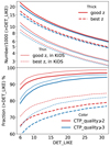 |
Fig. 1 Number of X-ray sources (upper panel) and fractions of sources (lower) resulted from counterpart quality and redshift quality selections. The red and blue lines indicate counterpart quality ⩾2 and ⩾3. respectively. The solid and dashed lines indicate good (zG ⩾3) and best (zG ⩾4) redshift measurements, respectively. The thick and thin lines indicate sources in the eFEDS 90%-area region and the KiDS region, respectively. |
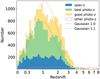 |
Fig. 2 Stacked filled histograms: redshift distributions of the eFEDS AGN with spec-z (5287; zG = 5; in blue), with best photo-z (9643; zG = 4; in green), and with good photo-z (6057; zG = 3; in yellow), respectively. The other AGN (1092; zG <3) are displayed in the magenta empty histogram. For sources with photo-z, the redshift PDF is used in plotting. For comparison, we plot the Gaussian distributions centered at z = 1.0 (green dotted line) and z = 1.1 (orange dotted line), which are normalized to the number of AGN with best redshift measurements (zG ⩾4) and good measurements (zG ⩾3), respectively. Both of them have σ = 0.15 in the space of log(l + z). |
2.2 Extraction of spectra
The observation mode of eROSITA is continuous scanning of the sky. This is different from previous large X-ray surveys, which were carried out with pointed observations in raster patterns. In scanning mode, a source moves across the field of view (FOV) multiple times rather than staying at a particular position in the FOV and the same position on the detector. Thus, during a scanning observation, each source is exposed to a local, effective exposure time corresponding to the duration of its passage in the FOV; during this effective exposure time, the source’s signal is subject to varying point spread function (PSF) and vignetting. The treatments of the data required by the eROSITA scanning mode are implemented in the eROSITA Science Analysis Software System (eSASS; Paper I). The raw eFEDS data are processed using the eSASS version eSASSusers_2112142. We use the task srctool, which creates spectral files of the OGIP format (OGIP/92-0073; OGIP/92–0024). We introduce here the eROSITA scanning-mode spectral extraction, taking eFEDS as an example.
2.2.1 Source and background regions
Source and background extraction regions are automatically defined by the versatile srctool task. The algorithm for building the extraction regions is described below. The extraction regions vary for each source depending on the source counts, background counts, and source extent model radius from the detection catalog. The local eROSITA PSF at 1 keV (PSF_ENERGY_KEV) is used throughout as the reference scale.
The source extraction region is chosen as a circle with a radius that maximizes the nominal signal to noise ratio (S/N) given the local background surface brightness, clipped to a minimum radius of 10” (MINIMUM_SOURCE_RADIUS parameter) and a maximum radius of the 99% energy enclosed fraction (EEF) radius of the PSF. To remove contamination of a nearby source from the source extraction region, we compare the surface brightness along the line joining the two sources and exclude a circular region around the contaminating source out to a radius where the PSF surface brightness of the confusing source is greater than 20% (MAX_CONF_MAP_TO_SRC_MAP_RATIO) of the target source surface brightness. It is clipped to a minimum of 5” and a maximum of 99% EEF radius. No exclusion zones are allowed to be centered within 10” (MINIMUM_EXCLUDE_DIST) from the source.
We adopt an annular background extraction region. An example is shown in Fig. 3. The inner radius is determined by increasing the radius step by step starting from twice (INITIAL_SRC_R_TO_BACK_R1) the source extraction radius until the target source’s surface brightness is less than 5% (MAX_SRC_MAP_TO_BG_MAP_RATIO) of the local background surface brightness, adopting a maximum of three times (MAX_RATIO_BACK_R1_TO_RADIUS_99PC) the 99% EEF radius of the PSF. With the inner radius determined, the outer radius determines the geometric area of the background extraction region. To sample the background spectrum with a good S/N in a sufficiently large area, we set the outer radius to a value corresponding to a background area that is 200 times5 (BACK_TO_SRC_AREA_RATIO) the source extraction area after excluding nearby sources from the background region. Similarly, to remove contamination of a nearby source from the background extraction region we calculate an exclusion radius where the contaminating source surface brightness is 10% (MAX_CONF_MAP_TO_BACK_MAP_RATIO) of the local background surface brightness. The exclusion radius is clipped to a minimum of 5” and a maximum of 99% EEF radius. Meanwhile, it is restricted to be smaller than the distance from the target source, so that in the case of a target point source inside a big cluster, a part of the diffuse emission of the cluster near the target source position will be included in the background (see Fig. 3 for an example). We further apply a maximum outer radius of 15’ to the srctool output, so that the background signal is always extracted near the source position.
Figure 4 displays the distributions of source (blue) and background (orange) extraction radii and spectra counts. We measure the spectral source counts in the 0.2–5 keV band instead of the full 0.2–8 keV band because most of the sources have no signal above 5 keV. Fainter sources have smaller source extraction regions to gain a better S/N and consequently smaller background extraction regions. The median of source radius, background inner radius, and background outer radius of the whole sample are (28”, 65”, 401”), respectively. If selecting only the sources with at least 10 or 30 spectral net counts in the 0.2–5 keV band, these median values are increased to (31”, 74”, 444”), and (41”, 100”, 588”), respectively. We adopted a large ratio (200) of background to source area to guarantee a well-sampled background spectrum with a large number of counts. For the full sample, the median number of 0.2–5 keV background counts is 873; selecting sources with source net counts > 10 and > 30 leads to median background counts of 1118 and 1956, respectively. For the full sample, 90% sources have at most 46% of the useful background spectral channels (20 ~ 900) empty. Selecting sources with source net counts > 10 and > 30, this maximum fraction of empty channel in 90% sources is reduced to 37% and 19%, respectively. The median 0.2–5 keV source net counts of the whole sample is 12. A total of 4946 (18%) sources have at least 30 0.2–5 keV source net counts.
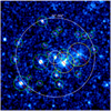 |
Fig. 3 Example of a background extraction region overlaid on the 0.2–2.3 keV image. For source 1702 (at the center), the background extraction region is defined by the area contained between the white annuli, after excluding nearby sources (circles with red stripes). The green and yellow circles indicate point- and extended sources, respectively. Physical scales are printed for the annuli and a source in terms of radii. |
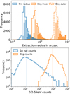 |
Fig. 4 Distributions of source (blue) and background (orange) extraction radii (upper panel) and distributions of source net counts and background counts in the 0.2–5 keV band (lower panel). The median values of the whole sample are marked with dotted vertical lines. The two-level shaded regions indicate the subsamples of the sources with source net counts ⩾10 and ⩾30, respectively. |
2.2.2 Creation of spectral products
Within the regions defined as above, the spectra are extracted from the event files using srctool. The spectral exposure time (the EXPOSURE keyword) is the total live time in which the extraction region is observed, not necessarily fully. In other words, it is the total deadtime-corrected exposure time of the good time intervals (GTIs) in which any part of the extraction region gets exposed in the FOV. In scanning mode, since a part of the extraction region is outside the FOV when the FOV enters or leaves the extraction region, the spectral exposure time is longer than the local exposure depth6. Such exposure incompleteness also manifests itself in the BACKSCAL keyword, which is the area (in square degrees) of the intersection of the extraction region with the FOV during the GTIs. It is smaller than the geometric area (the REGAREA keyword) of the extraction region in scanning mode, and the ratio between them can be considered as the inside-FOV fraction of the extraction region.
The redistribution matrix file (RMF) maps the energy space to the detector pulse height space. The same ground calibration is used to extract the RMF for all telescope modules (TMs; Dennerl et al. 2020). The ancillary response file (ARF) quantifies the exposed mirror area as a function of energy, taking into account the factors affecting the probability of an X-ray photon being captured, that is, the mirror vignetting effect, the CCD quantum efficiency, and the existence of bad pixels. Moreover, srctool also calculates the energy-dependent area-loss correction (CORRPSF) to the ARF as the fraction of source light falling inside the source extraction region and inside the FOV, as expected by the PSF-convolved source extent model, that is, a δ function in the case of this work focusing on point sources. This correction accounts for both the PSF enclosed energy fraction and the inside-FOV fraction of the source extraction region. The srctool calculates the total correction (CORRCOMB) that combines the vignetting and the area-loss correction in grids of time and space, that is, the source GTIs sampled in time steps of the nominal integration time (50 ms) and the effective (inside-FOV) source region sampled in steps of the detector pixel size (9.6”), and then sum them and apply the total correction to the ARF. In this work, since the extraction regions of point sources are compact and circularly symmetric, the vignetting is computed at the source center and assumed to be constant over the source extraction region to speed up the extraction.
In the eFEDS X-ray catalog (Brunner et al. 2022), sources with an extent likelihood EXT_LIKE< 6 are classified as unresolved. However, because of uncertainty in EXT_LIKE, a significant fraction of the sources with EXT_LIKE between 6 and 14 are in fact point sources (Liu et al. 2022b). Focusing on point sources in this work, we treat all the sources with EXT_LIKE< 14 as point sources in the spectra extraction by setting their source extent to zero. The original source extents were however used to define the extraction regions in Sect. 2.2.1.
In scanning observations like eFEDS, different sky positions correspond to different observing time, different exposure lengths, and different instrument responses. In the most rigorous case of spectral analysis, responses for the source and background regions should be computed separately to account for differences in the different positions. However, it can be simplified in this work. Because we extract background in an annulus region around the source and the annulus is not large, we consider the responses as identical in the source and background regions and thus only need to extract responses for the source regions. This assumption is more valid in scanning mode than in pointing mode, because in scanning mode, both the two regions move across the entire FOV multiple times so that the PSF and vignetting effects are both averaged similarly.
In general, the X-ray background varies also over time and space. However, the eROSITA background is relatively stable, with barely any background flare as commonly seen in the XMM-Newton observations (Predehl et al. 2021). Only one short background flare was found in the eFEDS observation and it was removed using the eSASS task flaregti (Paper I). Therefore, background variability between the source and the background regions is negligible. To make sure the source and background regions share the same background level, srctool extracts background signals only in the GTIs of the source so that the source and background spectra are always exposed at the same time7.
2.2.3 Spectra stacking
All seven roughly-identical TMs of eROSITA were activated for almost the entire eFEDS observation. For each source, srctool extracts a source spectrum, corresponding response files, and a background spectrum for each TM i. These are then summed. The combined spectrum is the equally-weighted sum of the spectra from the individual TMs. Given the exposure time Ti (the EXPOSURE keyword) for each TM, the exposure time of the combined spectrum is calculated as the mean of Ti over the seven TMs, with Ti = 0 for inactive TMs. The BACKSCAL of the combined spectrum is averaged over the active TMs.
The combined ARF is seven times the exposure-time weighted mean ARF of the active TMs

The combined RMF is the exposure and ARF weighted mean of the RMFs from the individual TMs. The weighting is computed individually for each energy bin.

Under this framework, inactive TMs (with Ti = 0) contribute to the combined ARF (through the factor 7) but not RMF. The combined ARF is always calculated as if all the TMs are activated.
3 Spectral analysis
Having the spectra files for each sources, we can now analyze them with astrophysical models. Our automated spectral analysis procedure first characterizes the total background emission empirically (Sect. 3.1), which is then jointly fitted with an astro-physical source spectral model (Sect. 3.2). The fitting procedure is described in Sect. 3.3, and following analyses on the spectral fitting results are described in Sect. 3.4, 3.5, and 3.6.
3.1 Background model
Background signals present in both the source and background regions. The source spectrum is composed of a source and a background component. We model the background spectrum and use the best-fit model shape together with the area scaling factor to account for the background component in the source spectrum.
The detected X-ray background partially corresponds to celestial X-ray photons focused by the mirrors and partially corresponds to secondary emission caused by soft or hard particles hitting the detector directly. The former is vignetted and the latter is not. To analyze the background spectrum, we have to model the vignetted component and the unvignetted component separately (see more discussions in Freyberg et al. 2020; Predehl et al. 2021; Liu et al. 2022b). However, this is not necessary for the present work, where we are interested in analyzing the source properties rather than the background. Intending to model the background in the source region, all we need is to rescale the two background components properly from the background region to the source region. We have chosen small source and background regions nearby to each other, and extracted both the source and background spectra in the source GTI. Thus they have exactly the same exposure time and approximately the same response. Therefore, both the vignetted and unvignetted background components can be rescaled using the ratio of BACKSCAL between the source and the background regions.
We use the automatic background fitting method described in the appendix of Simmonds et al. (2018) and implemented in BXA (Buchner et al. 2014). In this method, the background spectrum is modeled phenomenologically as a function of detector channels instead of energies. Briefly, principal component analysis (PCA) is run on the unbinned background spectra of all the eFEDS sources, after a log(1 + counts) transformation. The first six principal components (PCs) are then linearly combined to fit the background spectrum of each source. An individual background spectrum does not necessarily show all the features of the six PCs. Starting from the mean spectrum, PCs are iteratively added as long as the Akaike information criterion (AIC; Akaike 1974) of the fit is significantly improved. After finding the linear combination of PCs that describe the spectrum best, Gaussian lines are added (in count-space) as long as they improve the fit further. These added Gaussians can model features that might appear in some individual spectra and were missed by the PCA. Finally, the best-fit background model spectrum is converted into an XSPEC table model, which is dedicated only to this particular source. The model has a scale parameter, which should be set to the ratio between BACKSCAL of source and background when fitting the source spectrum. It also has a normalization parameter, which is expected to be unity in the simultaneous source and background fitting.
Figure 5 displays the best-fit background spectral shapes of the eFEDS sources as a function of energy channels. These spectral models are normalized to the mean value over the full range (between channel 20 and 900) and thus only show the variety of the background spectral shapes among the eFEDS sources. The background spectral shape is relatively stable across the four-day observation of eFEDS. The most variable part is at the softest energies below 1 keV (~ channel 150). For a small fraction of sources, one or more Gaussian components are added in addition to the PC A components. They appear as the features in the 3-σ upper percentiles of all the sources. For all the sources, the background over the full range has a mean and standard deviation of 5.3 + 0.3 counts s–1 deg–2. So, the background flux is also highly stable across the eFEDS field.
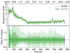 |
Fig. 5 Background model normalized to a mean value of 1. The red line displays the median of the models of all the sources, and the three-level green shaded regions indicate the 1,2, and 3 σ percentiles. The lower panel displays the ratio to the median. |
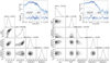 |
Fig. 6 Examples: posterior parameter distributions and spectra (inlaid at upper right) for an AGN (ID = 34) fitted with an absorbed power-law (left) and for a star (ID = 50) fitted with an APEC model (right). The posterior distribution of each individual parameter and each pair of parameters are plotted using the “corner” package (Foreman-Mackey 2016), with the median and 68% percentile interval around the median printed on top of each individual distribution. The spectral shape parameters for the absorbed power-law model include the slope (Γ) of the power-law and the logNH of the intrinsic absorber (in cm–2). For the APEC model, the spectral shape parameters include the Galactic absorption column density logNH, the temperature log KT (in ke V), and the abundance. All the normalization parameters (e.g., logPowNorm, logApecNorm) are measured in logarithm space. The background normalization parameter (logBkgNorm) is set free in the fitting and always equals one. In the spectral plot, the data (dark blue points) are rebinned just for representation to reach an S/N of 3 but allowing at most 6 adjacent bins (each bin includes 4 channels) to be grouped. The blue solid, dashed, and dot-dashed lines display the best-fit model folded with the instrument responses, the folded best-fit source model, and the best-fit background model rescaled to the source extraction region. The shaded region indicates the 99% percentile confidence interval of the model around the median. The lower panel compares the data with the best-fit model in terms of (data-model)/error, where the error is calculated as the square root of the model predicted number of counts. |
3.2 Source models
The sources are classified as galactic or extragalactic based on their SED or optical spectroscopy in Paper II. However, the classifications of a small fraction of sources are uncertain and may need to be revised as more data is obtained in the future. To allow for this, all sources are analyzed with a variety of physically motivated models appropriate for different source classes, and the derived properties are released as catalogs.
3.2.1 Stellar models
In the eFEDS catalog, 2695 X-ray point sources have reliable (CTP_quality⩾2) counterparts that are classified as “Likely galactic” or “Secure galactic” in Paper II. To account for them, we use a model of collisionally-ionized gas emission (APEC; Smith et al. 2001) at a redshift of 0 to fit the spectra in the 0.2–8 keV band. An example of spectral fitting results with this model is shown in the right panel of Fig. 6. We use a log-uniform prior between 0.05 and 5 ke V for the temperature and a log-uniform prior between 0.1 and 1 for the abundance. We also add a Galactic absorption with “TBabs” (Wilms et al. 2000). The Galactic column densities of these stars are allowed to vary in a narrow range between 4 × 10¹⁹ and 4 × 1020 cm–2 with a log-uniform prior. This model is called model 0 hereafter. It is the only model applied to galactic sources, as this work mainly focuses on the AGN, which comprise the majority of the eFEDS catalog.
3.2.2 AGN spectral models
Our baseline spectral model for AGN is an absorbed power-law, which is expressed as “powerlaw*zTBabs*TBabs” in the XSPEC terminology (see the left panel of Fig. 6 for an example). AGN spectra have a typical power-law slope Γ between 1.7 and 2.0, which varies depending on the sample selection (e.g., Nandra & Pounds 1994; Buchner et al. 2014; Liu et al. 2017; Ricci et al. 2017). To cope with the potential variety of spectral shapes, we adopt for Γ a Gaussian prior with a σ of 0.5, centered at 2.0 and truncated at –2 and 6, which can be expressed as Gaussian(2.0,0.5). Even though not being noninfor-mative, this is a weak prior in the sense that it is much broader than the intrinsic Γ scatter of AGN (e.g., Nandra & Pounds 1994; Liu et al. 2017). The prior center 2.0 is chosen based on the spectral fitting results of this sample (Sect. 4.4). The AGN intrinsic (rest-frame) absorption is modeled with “zTBabs” (Wilms et al. 2000). For its column density NH, a log-uniform prior is adopted between 4 × 10¹⁹ and 4 × 1024 cm–2. The range is sufficiently wide, extending to an unmeasurable low NH below the Galactic NH and an unmeasurable high NH in the Compton-thick regime. In all the models, we always apply a Galactic absorption (“TBabs”). The Galactic HI column density measured by HI4PI (HI4PI Collaboration 2016) in the eFEDS region is  (median and 1-σ interval). Based on the empirical correlation presented by Willingale et al. (2013), we compute the H2 column density for each source from the HI4PI NHI and the extinction E(B-V) measured by Schlegel et al. (1998) and then calculate the total Galactic NH for each source as NHI + 2NH2 The median total NH in the eFEDS region is
  (~12% higher than NH1).
The baseline model described above is called model 1: the “single-powerlaw” model. Considering potential additional emission component, such as the soft excess, the single-powerlaw model is a phenomenological description of the general spectral shape. It can be attributed to the inverse Comp-tonization in AGN’s hot corona only if the additional components are negligible, for example, in the case of obscured AGN. To fit potential soft excess, we add additional soft components to the single-powerlaw model (model 2 and 3) in the following section. To cope with low-count sources, a modified single-powerlaw model with the powerlaw slope fixed at Γ = 2.0 is also adopted and called model 4: the “Γ-fixed-powerlaw” model. A further modified variation, “shape-fixed-powerlaw” (model 5), is a simple, unabsorbed power-law (NH = 0) with Γ = 2.0 fixed. Models 1–4 are used to fit the broad-band (0.2–8 keV) spectra, but model 5 is used to fit the source detection band (0.2– 2.3 keV), where even the faintest sources are still detectable. These models are used for different purposes in this paper.
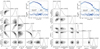 |
Fig. 7 Same as Fig. 6, but for an AGN (ID = 7) fitted with the “double-powerlaw” model (left) and the “powerlaw + blackbody” model (right), respectively. In addition to the power-law normalization (logPowNorm) and the background normalization (logBkgNorm), for the first model, the spectral shape parameters include the ∆Γ for the additional power-law, the Γ of the primary power-law, the logNH, and the flux ratio of the secondary to the primary power-law at 1 keV (logFrac); and for the second model, the parameters determining the spectral shape include the Γ of the power-law, the logNH, the log kT of the blackbody, and the blackbody normalization (logBBNorm). |
3.2.3 Multicomponent models
It is common to see deviations from a power-law in the X-ray spectra of AGN as observed by XMM-Newton and Chandra when the spectral S/N is sufficiently high. The most prominent feature is the soft excess in type-I AGN (e.g., Walter & Fink 1993; Bianchi et al. 2009). Such a soft component could be detected by eROSITA, which has a larger effective area, higher energy resolution, and a wider energy range (down to 0.2 keV) in the soft band than XMM-Newton. To model the spectra with soft excess, we use two double-component models to fit the broad-band (0.2–8 keV) spectra. The first one (model 2) adds an additional soft power-law to the single-powerlaw model, that is, “TBabs*zTBabs*(powerlaw+constant*powerlaw)”. The second one (model 3) adds an additional blackbody component, that is, “TBabs*zTBabs*(powerlaw+bbody)”. In both cases, we adopt the same prior as the single-powerlaw model for the primary power-law and the AGN absorption. Examples of these two double-component models are shown in Fig. 7.
Since the soft excess is usually well described by a black-body component with a temperature of 0.1 ~ 0.2 keV (e.g., Gierliñski & Done 2004; Crummy et al. 2006), in the “powerlaw + blackbody” model, we adopt a log-uniform prior between 0.04 and 0.4 keV for the temperature of the blackbody component. Because of Galactic absorption and the drop of telescope effective area at low energies, at a moderate S/N level, the soft excess can often be fitted by a power-law component too (e.g., Liu et al. 2017). This model is completely phenomenological, which can be used when the soft excess itself is of less interest than the primary power-law component. For a spectral model with multiple components, not only each model parameter requires a prior distribution, but two components also follow certain correlations of parameters (or distributions of relative parameters). The advantage of the “double-powerlaw” model is that, practically, it is very convenient to control the relative properties between the two power-law components. In our double-powerlaw model, we define the additional power-law with a ∆Γ parameter, which is the deviation of its slope to the slope of the primary power-law, and adopt for ∆Γ a uniform prior between 0.5 and 5. Setting such a positive lower boundary for ∆Γ the additional power-law is required to be significantly softer than the primary one. For the constant factor regulating the relative strength of the additional power-law, we adopt a log-uniform prior between 0.001 and 1. The upper boundary of 1 ensures that its 1 keV monochromatic flux is always lower than the primary one. For the powerlaw + blackbody model, it is not as simple to import such prior constraints. As a result, the two components are independent of each other, leading to high flexibility at the cost of a strong degeneracy. We remark that both the double-powerlaw model and the powerlaw + blackbody model are phenomenological. Especially, taking into account the AGN absorption, neither the absorbed soft power-law nor the absorbed blackbody component has a well-founded physical interpretation. Therefore, to measure the NH of obscured AGN, the single-powerlaw model is preferred over these double-component models.
With the soft excess modeled, the primary power law corresponds to a physical origin, i.e., inverse Comptonization in the hot corona. Our main goal of adding the soft excess component is not to study the soft excess component but to measure the properties of the primary power law. In addition to the primary power-law and the soft excess, a third component usually detected in AGN is a cold reflection, which becomes prominent mostly above 5 keV. However, eROSITA’s effective area drops drastically above 2.3 keV. Also because of the relatively-high particle background, almost all the eFEDS sources have barely any signal above 5 keV. Therefore, adding a cold reflection component does not impact our results. Limited by data quality, the double-component models are our best approach to achieve a reasonable constraint on the intrinsic properties of AGN. They are sufficiently flexible to describe almost all the eFEDS spectra (see the fit goodness discussion in Sect. 4.2).
3.3 Spectral fitting procedure
The XSPEC software (Arnaud 1996) is used to load the spectra files and calculate the Poisson likelihood (C statistic, Cash 1979) for each set of parameters. We fit the source and background spectra simultaneously, modeling the background spectrum with the background model (see Sect. 3.1), and modeling the source spectrum with a source model convolved with the X-ray responses plus the background model convolved with a diagonal matrix response. In addition to the parameters of the source model, the background model adds an additional normalization parameter, which is expected to be unity but let free to vary.
A Bayesian spectral fit is performed with BXA8 (Buchner et al. 2014; Buchner 2021), which connects XSPEC with the UltraNest9 nested sampling package (Buchner 2021). Given a prior distribution for each parameter of the model, the robust MLFriends algorithm (Buchner 2016, 2019) implemented in UltraNest explores the whole parameter space and samples equal-weighted (same probability) points. These points represent the posterior distributions of the model parameters (as illustrated in Figs. 6 and 7).
From the posterior distribution of each parameter, we measure the median and the 1-σ percentile confidence interval around the median, i.e., the 68% percentile equal-tailed interval. For values inferred from the spectral parameters, such as flux and luminosity, we also obtain the posterior distribution and calculate the median and 1-σ percentile interval similarly from the posterior distribution. From the posterior sample, we can also select the point with the maximum likelihood as the “best-fit”, as it is similar to the best-fit found by maximum-likelihood methods. This best-fit is reported in our spectral property catalog but only used for visualization (Figs. 6 and 7) and fit goodness evaluation (Sect. 4.2). In other analyses, we always adopt the Bayesian interpretation.
The Bayesian method, in combination with the background modeling, does not require rebinning of the data. However, to speed up the fitting of a large number of sources, the spectra are regrouped four-fold, i.e., grouping every four channels into one, since a high energy-resolution analysis of narrow line or edge features is out of the scope of this work and has negligible impact on our results.
3.4 Constraints on the spectral shape
Many sources have too few counts to constrain the parameters regulating the shape of the spectral model, such as NH and power-law slope Γ. To explore the spectral-shape constraint power of eROSITA spectra, we develop and present our criteria to objectively measure the constraints on the spectral shape following two approaches.
In the first approach, in addition to the equal-tail percentile interval, we also calculate the highest-density interval (HDI) from the posterior sample. The median and confidence interval are reasonable measurements of a parameter only if the parameter domain is wide enough to allow the PDF to drop toward zero at both the boundaries of the range. This requirement can be easily met for a well-constrained parameter like the normalization, but not for NH– its PDF does not drop toward lower values in the case of an unobscured AGN. The percentile interval can be calculated in all cases, regardless of the PDF shape. However, in such cases where the PDF monotonically increases toward lower values, the HDI lower limit does not exist and thus will be pegged at the lower boundary. This is an indicator of no absorption. To calculate HDI with better accuracy, rather than using the posterior sample of a parameter directly, we first smooth the distribution using Gaussian kernel density estimation (KDE) with a minimum bandwidth of 0.1. The kernel is renormalized to take into account only the part of the kernel within the domain. Then we extract 10 000 points following the smoothed distribution and use them to calculate the HDI limits.
In the second approach, we quantify how much the posterior distribution of a parameter differ from the prior using the Kullback-Leibler (KL) divergence for a parameter X,

For uniform or log-uniform prior, the comparison is made in the full parameter range; in the case of a Gaussian prior (for power-law slope), the comparison is made within the 3-σ range. This KL value is a measurement of information gain from the data in units of nats10. A small value of KL means the posterior is the same as the prior and thus the posterior gains little information from the data. A large value of KL means a significant difference between the posterior and the prior, which is attributed to the constraint provided by the data. Based on the KL divergence and the HDI confidence interval, we quantify the constraint for each AGN on NH and Γ of the single-powerlaw model in Sect. 4.3.
3.5 Flux and luminosity measurements
We present a measurement of the observed fluxes in the 0.5– 2 keV and 2.3–5 keV bands for all the X-ray sources. The 2–10 keV fluxes are not measured because eROSITA data has a small effective area and a high background at >5 keV11. The observed fluxes can be accurately measured from X-ray spectra as long as the spectra are well fitted by the model. We choose the 0.5–2 keV fluxes measured with the most appropriate models as follows and assign a FSModel flag for the flux measurement of each source. Firstly, for bright sources, mul-ticomponent models are preferred because they could describe the spectral shapes better. For the AGN with at least 20 net counts, we adopt the soft-band fluxes measured with the pow-erlaw + blackbody model (model 3) and flag it FSModel = 3 (7007 sources). Secondly, for the faint AGN with less than 20 net counts, multicomponent models are not meaningful. We perform a narrow-band fitting in the 0.4–2.2 keV (slightly broader than 0.5–2 keV) with the single-powerlaw model and call it model 6. We adopt the soft-band fluxes measured with this model and flag them FSModel = 6 (15984 sources). Thirdly, for 2572 stars (CTP_quality ⩾ 2 and CTP_class ⩽ 1), we adopt the soft-band fluxes measured with APEC model (model 0) and flag them FSModel = 0. All the other sources are considered as AGN. At last, regardless of the models adopted above, when the measured 1-σ percentile interval width of flux is larger than three orders of magnitude or when the source has less than three net counts in the 0.5–2 keV band, we consider their fluxes as un-measurable from the spectra. We adopt the fluxes measured with the shape-fixed-powerlaw model (model 5) and flag these 2347 sources as FSModel = 5. This model is applied to the source detection band (0.2–2.3 keV), which guarantees that the source signal is detectable. Such flux measurements are based on broadband photon counts rather than spectra. The other three classes (FSModel 3, 6, or 0) are spectra-based measurements that are more robust and accurate.
Since eROSITA is much more sensitive in the 0.2–2.3 keV band than in the band above 2.3 keV, the broad-band fitting is dominated by the soft band signal. Therefore, it provides an accurate flux measurement in the soft band but not necessarily in the hard band. To measure the 2.3–5 keV fluxes, we apply the single-powerlaw model in the 2.3–8 keV band and call it model 7. Most of the eFEDS sources are undetectable in the hard band, so we adopt the hard-band flux measurements with model 7 for the 1354 sources with the 1σ percentile interval width of flux smaller than three orders of magnitude and with at least three net counts in the 2.3–5 keV band. They are flagged as FHModel = 7. For the other 26556 sources, we adopt the 2.3– 5 keV fluxes measured using the shape-fixed-powerlaw model (model 5). Such a hard-band flux, classified as FHModel = 5, corresponds to extrapolating of the source signal in the source-detection band (0.2–2.3 keV) but not any hard-band detected signal. Only the hard-band fluxes with FHModel = 7 can be considered as robust spectra-based measurements.
Using a serial of models, we computed the intrinsic (absorption-corrected) luminosities of the AGNs in two soft energy bands, 0.5–2 keV and 1.999–2.001 keV. The latter band is used to calculate the monochromatic luminosity at 2 keV. In the cases of double-component models, the soft-excess component is included in the luminosity measurement. The most appropriate model is chosen to present the X-ray luminosity of each source in Sect. 4.5. Since most of the sources have low S/N in the hard band, the 2–10 keV luminosities are not presented in this work. They are only presented in Nandra et al. (in prep.) for the eFEDS hard-band selected sources.
3.6 Sample distributions
Most of the eFEDS sources have a low number of photon counts and thus poor spectral constraints. The measured spectral parameters have large uncertainties and, in some cases, substantial degeneracies, for example, between the column density and the photon index. Nevertheless, we aim to produce parameter distributions for the column density and the photon index.
A suitable method to propagate uncertainties and learn a sample distribution in this setting is Hierarchical Bayesian models (HBM). For a spectral parameter x, such as NH or Γ, we assume that the true values of the sources follow a Gaussian distribution N(x|µ, σ) with a specific mean µ and a standard deviation σ. This is the parent distribution that corresponds to a given sample with certain selection biases, not corresponding to any physical AGN population. For each source i, the parameter x is drawn from this parent distribution, and the combined likelihood for its data Di is
 (1)
(1)
where P(x|Di) and P(x) are the posterior and prior distributions in the spectral fitting. Adopting a uniform prior for x in a broad range, the P(x) can be dropped from Eq. (1). Then multiplying the likelihood of all the sources into a combined likelihood:
 (2)
(2)
it forms a Bayesian inference problem about N+ 2 parameters, i.e., the µ and σ parameter of the parent distribution and one x parameter for each of the N sources. Instead of fitting all the data simultaneously to derive all these N + 2 parameters, we simplify the problem to two parameters using the numerical approach described in Baronchelli et al. (2020). Since for each source i, we have obtained a posterior sample xi,j that approximate the posterior distribution P(x|Di), we can integrate out the x parameter of each source using a Monte Carlo integration method, i.e., importance sampling, turning Eq. (2) into:
 (3)
(3)
For each object, we select 1000 values from its posterior sample. The Gaussian probability density of the parent distribution is evaluated and averaged at these values, and then multiplied for all the sources to obtain the combined likelihood. Assuming flat priors on µ and log σ, their posterior distribution can be explored through nested sampling. It is done using the PosteriorStacker12 python tool, which internally also uses the nested sampling tool UltraNest. Although this approach does not fit all the data simultaneously, it determines the two parent-distribution parameters simultaneously with the spectral parameters of the N sources, since the N parameters are used as random variables, which are integrated out rather than inferred as the two parent-distribution parameters. It is necessary that the posterior samples of x are obtained under flat priors (e.g., for logNH). For parameters where this is not the case (the photon index Γ), the posterior samples are first resampled according to the inverse of the prior.
Beyond a Gaussian model, PosteriorStacker also implements a nonparametric histogram model. In this model, bins are allowed to vary their densities. A flat Dirichlet prior on the bin densities assures that the sample distribution sums to unity. This histogram model allows investigating the sample distribution without assuming a specific (e.g., symmetric, mono-modal) model shape.
We remark that the method above only propagates the parameter uncertainty of each source to construct a sample parameter distribution, but does not make any correction to the sample selection bias. Therefore, the obtained distribution represents only the property of this sample but not any intrinsic property of AGN (see more discussion in Sect. 4.4).
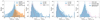 |
Fig. 8 Model comparison on the basis of Δ log Z between pairs of models, i.e., 1) the single-powerlaw (pw) model vs the APEC model; 2) the double-powerlaw (pw+pw) model vs the single-powerlaw model; 3) the powerlaw + blackbody (pw+bb) model vs the single-powerlaw model; 4) the powerlaw + blackbody model vs the double-powerlaw model. The empty histogram indicates all the sources and the filled histogram corresponds to the subsamples of bright sources with at least 20 net counts in 0.2–5 keV band. In the first panel, the blue and orange colors indicate AGN and stars respectively. In the second and third panels, the red color indicates the subsamples of AGN with a median logNH above 21.5. In the last panel, the blue and magenta colors indicate sources with log Zapec − log ZpW below and above 1.3 respectively. |
4 Results
4.1 The spectral property catalog
We present the AGN catalog selected from the eFEDS X-ray sources. In addition to the AGN catalog, we also present the basic spectral properties of all the eFEDS X-ray sources, such as spectra extraction information, count rate or flux of source and background. We performed spectral fitting with eight models (model 0~7) and present the spectral fitting results using all the models. Some redundant information is provided here, which might be useful in the future when further multiband follow-up enrich or correct the current optical-counterpart identifications of these sources. Table 1 lists the ten tables presented with this paper, including the AGN catalog, the basic spectral property catalog, and the spectral fitting results of the eight models. These tables are available on the eROSITA early data release website13 and at the CDS, and the table columns are described in Appendix B. In this section, we analyze the spectral fitting results adopting the most appropriate models for different purposes.
4.2 Fit goodness and model comparison
As most of the eFEDS sources have a low S/N, goodness of fit is not relevant for them, because such sources are already over-fitted by the model. To test the fit goodness for a small number of the brightest sources, we calculate the x2 statistic as follows. We rebin the source spectrum to guarantee at least 25 counts in each bin, and then calculate the x2 value for the rebinned spectrum against the best-fit model. The fit goodness can be judged by comparing the x2 value with a x2 distribution of the degrees of freedom (DOF) of the rebinned spectrum. For most sources, the rebinned spectrum has no DOF at all. Using the double-powerlaw or the powerlaw + blackbody model, only 86 AGN have at least 10 DOF, out of which only ten have x2/DOF> 1.5 and only two have x2/DOF> 2. We find that the main reason for such large x2/DOF is narrow emission or absorption features rather than broad-band spectral shape curvature. Therefore, these data do not need a model that is more complex than our double-component models.
Considering the low S/N of most sources, model comparison is not relevant for them either. Here, we compare the models but not in order to select the most appropriate model for each source. We only make a rough comparison at the sample level and look for cases where the data is powerful enough to reveal an additional component (soft excess).
BXA calculates the logarithmic Bayesian evidence log Z for each fit. A relatively larger value of logZ can be used as a model preference indicator (Buchner et al. 2014). As displayed in Fig. 8, at the catalog level, stars prefer the APEC model over the power-law model, i.e., logZAPEC > logZpowerlaw, and AGN favor the power-law model. However, the preference is only significant (e.g., ΔlogZ >1) in a small fraction of sources, because of the S/N limitation. A few cases of misclassification might exist among the small number of AGN that favor the APEC model and the small number of stars that favor the power-law model.
Comparing the single-powerlaw model with the double-component models, the ∆ log Z show a significant tail in favor of the flexible double-component models, indicating the existence of soft excess. Because of low S/N, a majority of the sources reside in the peak around ∆ log Z = 0, especially for sources with less than 20 counts. The AGN with a posterior median logNH above 21.5 have ∆ log Z ~0 because soft excess is irrelevant in such cases.
Comparing the powerlaw + blackbody model and the double-powerlaw model, the ∆ log Z distribution is only slightly above 0. They have the same number of parameters, but the power-law + blackbody model is more flexible. The double-powerlaw model is restricted to the cases with a soft excess that is softer (∆Γ always >0.5) than the primary power law and weaker than the primary power law at 1 keV. However, the blackbody component is free to be stronger than the primary power law in the model. We select 255 AGN with log ZAPEC − log Zpowerlaw > 1.3 as a special class and call them APEC AGN since they favor the APEC model. As displayed in Fig. 8, the APEC AGN favor the blackbody model, because the spectral shape of hot plasma emission is more similar to blackbody than power law. For the other, normal AGN (called power-law AGN in the figure), the double-powerlaw model and the powerlaw + blackbody model could fit the data equally well.
Catalogs presented in this work.
4.3 Constraints on NH and power-law slope
In this section, we quantify the constraints on NH and Γ for each AGN based on the single-powerlaw model. Compared with the power-law slope Γ, a varying NH changes the overall broadband spectral shape more prominently. To quantify whether NH is measured by the eROSITA data, we use logNH,HDI,lower and KLNH to divide the NH measurements into four classes (NHclass in the catalog) as follows. At a low KLNH (e.g., < 0.3), the 68% interval widths are large and close to 68% of the parameter range (purple arrowed lines in Fig. 9). We call them class (1) − uninformative sources, as no information about NH is gained from the data. The posterior NH distribution of an example source (ID = 878) is displayed in Fig. 9.N4 in cyan. As shown by the median NH distribution in Fig. 9.N5, fluctuation tends to bring the median NH of an uninformative source to a large value in the middle of the parameter range, but such values should not be adopted as meaningful measurements. The class (2) is comprised of the sources with HDI lower limit logNH,HDI,lower pegged at the parameter lower boundary (4 × 1019 cm–2), practically adopting logNH,HDI,lower<19.8. With the posterior NH distribution monotonically increasing toward lower values, such sources are classified as unobscured. The posterior NH distribution of an example source (ID = 4526) is displayed in Fig. 9.N4 in green. The median NH of such sources, which should not be used either, show a strong correlation with the KLNH, which is nothing but a boundary effect. This boundary effect is the strongest in these HDI-pegged cases, but also exists in other cases (Fig. 9.N2) where the NH uncertainty is not narrow enough to clearly separate the highest-density part of the PDF from the lower boundary (see an example source, ID = 20, in orange color in Fig. 9.N4). The HDI lower limits of such sources are measurable but inaccurate because of the boundary effect. To distinguish between such sources and the sources with well-constrained NH lower limits (see an example source, ID = 7274, in red color in Fig. 9.N4), we adopt a criterion logNH,crit = 20.2–2 log KLNH (green line in Fig. 9) and compare it to the 1-σ HDI lower limit logNH,HDI,lower. Sources with logNH,HDI,lower below and above logNH,crit are assigned to class (3) − mildly−measured and class (4) − well-measured, respectively. Such a criterion represents a natural selection bias against the measurement of low NH when the constraining power (KLNH) of the data is low. We note that the well-measured class is defined in the sense that absorption is significantly detected, irrespective of the measured NH value, which can be as low as 1020 cm–2. When a sample of AGN that are obscured at a certain level is needed, we recommend selecting the well-measured and mildly-measured sources with logNH above a threshold of 21.5 or 22. The NHclass has nothing to do with NH uncertainty width either − an obscured AGN selected as above with well-measured NH could have a wide posterior distribution and thus a huge NH uncertainty.
For the sources with uninformative NH, we do not expect to extract any spectral information from the data. Figure 10 displays the fractions of each of the four classes as a function of the 0.2–2.3 keV source detection likelihood and the fractions of sources with robust luminosity measurements (discussed later in Sect. 4.5). To suppress the fraction of uninformative NH measurements to below 5%, a detection likelihood > 10 is required. To suppress this fraction to 1%, a detection likelihood > 18 is needed.
Similarly, the KL divergence for the power-law slope,  , measures how significant the posterior Γ distribution differs from the prior Gaussian(2.0,0.5) distribution. The panels G1~G3 of Fig. 9 display the distributions of the posterior Γ and the KLΓ, dividing the sample into three according to the Γ HDI interval width. When KLΓ <0.3, there is barely any information imported from the data, as the posterior and prior are similar or even identical (see an example, ID = 864, in Fig. 9.G4). As displayed in Fig. 9.G5, such sources comprise a majority of the eFEDS sources (82%), which concentrate in the peak around 2.0, the prior center. In the median Γ range of 2.0 ± 0.3, 95% of the sources have KLΓ <0.3. As displayed in the panels G1 and G2 of Fig. 9, the Γ of such sources have large uncertainties, which can be as large as the prior width (magenta arrowed lines) in the worst cases. To avoid huge uncertainties in their measurements of NH and luminosity, we might as well adopt a stronger prior in the fitting by fixing Γ at 2.0.
A high KLΓ can be attributed to two causes. One cause is a small uncertainty of Γ, in other words, the posterior PDF is narrower than the Gaussian prior with a scale of 0.5. The PDF of an example source (ID = 471, in purple solid line) is displayed in Fig. 9.G4. As displayed in Fig. 9. G3, all the sources with Γ error width below 0.55 have KLΓ >0.3. The second cause is a significant offset of the measured Γ from the prior center 2.0, as shown by the two branches in the Γ-KLΓ plots extending to very-large and very-small Γ at high KLΓ and by the bimodal distribution of median Γ (purple filled histogram) in Fig. 9.G5. The posterior PDFs of two example sources (ID = 13651 in purple dashed line and ID = 595 in purple dotted line) are displayed in Fig. 9.G4. With our Gaussian prior, the KLΓ >0.3 criterion selects all the sources with abnormal slopes. A large fraction of these sources (45%) have median Γ >2.4, and a small fraction (6%) have median Γ < 1.6. The main reason for the steep slopes is the existence of soft excess. Adding an additional soft-excess component, such steep slopes will be largely reduced (Sect. 4.4). The flat-slope sources might correspond to an intrinsically hard spectrum. However, their flat slopes might also be a result of the inappropriate model. For sources with ionized, partial-covering, or Compton-thick absorbers, our single-powerlaw model with a neutral absorption leads to a flat slope. The small uncertainties and abnormal slopes are the information gained from the data. Regardless of the cause, the information should be adopted and thus the Γ parameter must be set free in the fitting of these cases.
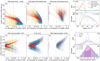 |
Fig. 9 Distributions of the posterior median and 1-σ HDI interval as a function of KL divergence for NH (panels N1~N3) and for power-law slope Γ (G1~G3), respectively, as measured using the single-powerlaw model. Examples of source posterior PDF are compared with the prior PDF for NH (N4) and for Γ (G4). The distributions of posterior median values are also displayed for NH (N5) and Γ (G5), respectively. The HDI intervals are plotted as blue error bars for the sources with at least 30 net counts and yellow error bars for the other faint sources. For representation, we only plot the yellow error bars for a random 10% of these faint sources. In panels N1~N3, the AGN catalog is plotted separately in three groups, i.e., N1: sources with the HDI lower limit truncated by the boundary (<19.8); N2 and N3: other sources with the HDI lower limit below and above the green line, which corresponds to logNH = 20.2–2 log KLNH. In panels G1~G3, the catalog is also divided into three, i.e., sources with HDI interval width >0.8 (G1), between 0.55 and 0.8 (G2), and <0.55 (G3). The purple arrowed lines indicate 68% of the NH parameter range at one side of the boundary (N1) or at the center of the range (N2, N3). The magenta arrowed lines indicate the 68% range of the Gaussian(2.0,0.5) prior for Γ. In panels N5 and G5, the blue empty histograms indicate the whole AGN sample; the cyan, green, orange, and red colors indicate the four classes of NH measurements, i.e., 1) uninformative, 2) unobscured, 3) mildly-measured, and 4) well-measured; the purple and magenta colors indicate sources with KLΓ above and below 0.3. In panels N4 and G4, the black lines indicate the prior PDFs; the IDs of example sources for NH PDF are 878 (cyan), 4526 (green), 20 (orange), and 7274 (red); the ID of example sources for Γ PDF are 864 (magenta), 13651 (purple, dashed), 595 (purple, dotted), and 471 (purple, solid). |
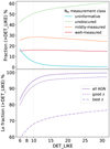 |
Fig. 10 Fractions of sources selected by X-ray spectral properties among the AGN detected in the eFEDS 90%-area region as a function of the 0.2–2.3 keV source detection likelihood. In the upper panel, concerning the NH measurement with the single-powerlaw model, the AGN are divided into four classes, i.e., 1) uninformative (cyan), 2) unobscured (green), 3) mildly-measured (orange), and 4) well-measured (red). In the lower panel, the purple lines indicate the AGN with spectral measurements of LX (discussed in Sect. 4.5), and the solid, dashed, and dash-dotted line styles indicated all the AGN, the AGN with good red-shift measurements, and the AGN with the best redshift measurements, respectively. |
4.4 Spectral properties of the sample
The upper panel of Fig. 11 displays the distribution of NH measured with the single-powerlaw model. The posterior median NH shows a wide distribution (filled histogram). As discussed in Sect. 4.3, these median values should not be used directly without checking the NHclass first. In most cases, the median NH is dominated by fluctuation. Only in the well-measured cases (NHclass = 4; red histogram in Fig. 11), where both the lower limit and the upper limit of NH are well measurable, can the median value be safely considered as a good proxy of the real NH. Thanks to the power of the Bayesian method, in some cases with fewer than 20 net counts (the overlapping between red and blue histograms in Fig. 11), we obtain NH measurements (NHclass = 4), although such measurements have huge uncertainties. In such low-count cases, NH is only measurable when it is high enough to cause a significant hardness of the spectral shape. In other words, the NHclass = 4 selection biases for highly-obscured AGN. Moreover, high NH values measured in low counts cases should be treated with caution, because of the limited spectral model (without considering partial-covering or ionized absorption) and potential, additional uncertainties induced outside the spectral fitting, for example, in the spectra extraction or background estimation.
Based on the posterior median NH, the obscured AGN with logNH >21.5 (3128 sources) and logNH > 22 (1568 sources) comprise 15% and 7% of the AGN with goodredshifts. However, these fractions are biased high because the obscured sources have wider PDFs than the unobscured ones, and a substantial fraction of their PDF resides in the unobscured regime. To account for the asymmetric and large uncertainties, we run the numerical HBM method (Sect. 3.6) to measure the intrinsic NH distribution of the sample. We adopt the nonparametric histogram model for the NH distribution, where there is no assumption on the shape of the distribution. All the AGN with good redshift measurements are involved in the HBM calculation, including the uninformative ones, which practically have no impact on the results. The inferred NH histograms are normalized to the sample size in Fig. 11 for comparison with the median NH distributions. The intrinsic distribution is largely dominated by unobscured sources. Based on the HBM inferred histogram, the fractions of obscured AGN with logNH >21.5 and logNH >22 are 8% and 4%, respectively. Selecting the sources with at least 20 counts, the obscured fractions are even lower, which are 3.4% and 1.6%, respectively. Such low obscured fractions are because eROSITA has a much larger effective area in the soft band (< 2.3 keV) than in the hard band, and the X-ray sample selection is dominated by the soft band. Liu et al. (2022b) simulated the eFEDS source detection in detail and presented mock eFEDS catalogs that are highly representative of the real one. Using their input mock AGN catalog, we plot the fraction of detected sources as a function of AGN NH in the lower panel of Fig. 11. It displays the selection bias against obscured AGN, which is more severe at low redshifts.
We also remark that the peak of the HBM-inferred NH distribution at the lower boundary cannot be quantitatively accurate. This is because, for unobscured AGN, the posterior NH PDF, which does not decrease toward lower NH, is dependent of the chosen lower boundary. The potential bias caused by the lower boundary is also propagated by the HBM method to the NH distribution. At logNH < 1021 cm−2, we can only derive the integrated fraction from the NH PDF but not any detailed PDF shape in finer bins.
In Fig. 12, we compare the slopes of the primary power-law measured using the powerlaw + blackbody model and the single-powerlaw model. With the single-powerlaw model, the power-law slopes indicate the overall slopes of the spectra. Having the soft excess fitted with the blackbody component, now the slopes correspond to an intrinsic property of the power-law emission from the X-ray emitting coronae. As displayed in Fig. 12, the steep-slope sources move significantly toward lower values, largely eliminating their deviation from the typical slope of 2.0. With a larger logZpw+bb–logZpw, the soft excess component is more significantly detected, and the affection on the power law slope is larger.
We use the HBM method to derive a Gaussian distribution of the power-law slope measured by the powerlaw + blackbody model from all the AGN with good redshifts. We obtain a mean value of 2.07 and a standard deviation of 0.24. If using the double-powerlaw model, the mean and standard deviation of the Gaussian Γ distribution are 1.98 ± 0.20. Compared with hard-band selected AGN samples (e.g., Liu et al. 2017), the typical slope of the eFEDS AGN is relatively steeper. It reflects the selection bias of the eFEDS sample for AGN with steep slopes or with strong soft excess. The HBM method does not correct for the bias, it inherits the bias and might even aggravate it. Considering eROSITA’s large effective area in the soft band, the steep-slope sources tend to have better S/N and thus tighter constraints on Γ. As a consequence, they might contribute to the HBM inferred Γ distribution with relatively higher weights. In our spectral models, including the single-powerlaw model, we always adopt for Γ a Gaussian prior that is centered at 2.0 but with a much larger scale (0.5) than the HBM-measured one (0.24). Catalog-wise, this is a relatively-unbiased, weak prior, which compromise between gaining a physically reasonable spectral modeling and covering a wide span of spectral shapes in such a large catalog.
To select sources with soft excess detected, we can adopt a typical threshold of logZpw+pw–log Zpw > 1 based on the double-powerlaw model, or adopt logZpw+pw–log Zpw > 1 based on the powerlaw + blackbody model (Buchner et al. 2014). The two selections result in a number of 144 and 224 AGN, respectively. The blackbody temperature and NH of these sources measured through the powerlaw + blackbody model are displayed in Fig. 13. Thanks to the prior limits that we put onto the double-powerlaw model, i.e., the soft power-law must be softer and weaker (at 1 keV) than the primary power-law, this model only identifies soft excess in unobscured AGN. With an unlimited relative strength, the powerlaw + blackbody model identifies more soft excesses with higher temperatures at higher NH. Such soft excesses in terms of obscured blackbody are suspicious and are likely due to over-fitting.
The double-powerlaw model has a relative strength parameter. Using the posterior median parameter values, we also calculate a relative strength for the powerlaw + blackbody model, i.e., the ratio between the blackbody component and the power-law component at 1 keV. We compare this blackbody relative strength with the posterior median relative strength parameter of the double-powerlaw model for the AGN with good red-shifts and at least 20 net counts in the upper panel of Fig. 14. In the lower panel of Fig. 14, we also compare the primary power-law slopes measured by these two models. Unlike the relative strength of the soft power law, which is limited between 0.001 and 1, the blackbody relative strength extends to much-lower and much-larger values. There are a significant number of sources with a blackbody relative strength > 1 or even > 10. With the double-powerlaw model, which does not allow such strong soft excess, such sources tend to be fitted with a steep primary power-law. With a high soft-excess relative strength, the soft excess becomes the dominant component of the spectrum; also considering eROSITA’s low effective area in the hard band, the primary power-law component could become negligible. In fact, such sources are better described by a blackbody-like model rather than a power-law model, and thus their classification of AGN is suspicious, although in some rare cases, AGN’s corona emission might shut down, leaving only a soft component (e.g., 1H 0707–495 Boller et al. 2021). Considering only unobscured AGN with NH below 1020 5 cm−2 (filled blue histogram), the cases of over-strong blackbody are largely eliminated, indicating that they are more likely a result of over-fitting. The remaining cases of strong blackbody components are few, most of the sources show an opposite behavior with much lower blackbody relative strengths below the lower boundary of the soft-powerlaw relative strength. As a result, and also because of the intrinsically different spectral shape between blackbody and power-law, the power-law slope measured by the powerlaw + blackbody model is 4% (median) higher than that measured by the double-powerlaw model. Broadly speaking, the two models give rise to similar results for typical AGN. To guarantee all the sources in this large sample with various spectral shapes can be fitted well, in this work, we adopt the flexible powerlaw + blackbody model in the analysis below. Our main goal of adding the soft excess component is only to fit the broad-band spectral shape better. More detailed discussions about the soft excess itself are presented in Waddell et al. (in prep.).
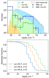 |
Fig. 11 Upper panel: NH distribution of the eFEDS AGN with good redshifts (zG ⩾3). The stacked filled histograms display the median NH distributions of the AGN with 0.2–5 keV net counts >200 (196 sources; yellow), >20 (6181; yellow and green), and >0 (20987; yellow, green, and blue). The red empty histogram displays the median NH of the sources with well-measured NH (NHclass = 4). The blue and green empty histograms (with 1-σ errorbars) present the inferred intrinsic NH distribution using the HBM method for all the AGN with good redshifts (20987) and the subsample with at least 20 counts (6181), respectively. Lower panel: detected fraction measured by simulation as a function of NH for three subsamples of AGN with 2–10 keV intrinsic luminosity Lx above given logarithmic thresholds and redshift below given thresholds. The three Lx thresholds are selected such that the three subsamples have similar detected fractions at the lowest NH. |
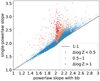 |
Fig. 12 Comparison between the posterior median power-law slopes measured using the single-powerlaw (pw) model and the powerlaw + blackbody (pw + bb) model for all the AGN with good redshifts. The sources with logZpw+bb–logZpw below 0.5, between 0.5 and 1, and above 1 are plotted in blue, orange, and red, respectively. |
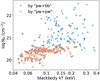 |
Fig. 13 Distributions of the blackbody temperature and NH measured by the powerlaw + blackbody model for the AGN with soft excess identified through the powerlaw + blackbody model (pw+bb; blue) and the double-powerlaw model (pw+pw; orange), respectively. |
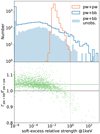 |
Fig. 14 Upper panel: distributions of the soft-excess relative strength measured by the powerlaw + blackbody model (blue) and the double-powerlaw model (orange), respectively, for the AGN with good redshifts and at least 20 net counts. The values are clipped at a lower limit of 10−6. The blue filled histograms indicate an unobscured subsample with the NH measured by the powerlaw + blackbody model below 1020.5 cm−2. Lower panel: ratio between the slopes of the primary power-law measured by the two models for the unobscured subsample as a function of the blackbody relative strength. The green horizontal line indicates the median value (1.04) of the ratio. |
4.5 X-ray luminosities
We have measured the absorption-corrected luminosity Lx in the 0.5–2 keV band and at 2 keV using a few spectral models. Among the used models, we choose the most appropriate one to present an LX for each AGN based on two principles: 1) adopting weaker spectral-shape priors for high-quality data and stronger spectral-shape priors for low-quality data, so that high-quality data provides accurate measurements through flexible, multicomponent spectral modeling and low-quality data provides usable measurements based on reasonable assumptions on typical AGN spectral shape; 2) avoiding over-modeling of multicomponent models to obscured sources, in which the strong degeneracy between the absorption and the soft excess causes superfluous uncertainty in the absorption correction to Lx.
The selection is done as follows. Firstly, when the NH parameter of the single-powerlaw model is unconstrainable, i.e., NHclass is uninformative, we consider the data quality as too low for a reasonable spectral fitting. For these 4889 sources with the worst data quality, we adopt the strongest prior, i.e., using shape-fixed-powerlaw model (model 5) to calculate LX. Rather than a spectral measurement, such an LX is in fact a counts measurement based on a strong assumption on the spectral shape, ignoring the spectral shape uncertainty. These LX measurements are presented in the catalog but excluded from further analysis in this paper. Secondary, for sources with KLΓ < 0.3 (15965) in the single-powerlaw model, the data quality is still relatively low and their power-law slope Γ are consistent with the assumed Gaussian prior centered at 2.0. We adopt a strong prior for them and use the T-fixed-powerlaw model (model 4) to compute LX. At last, for the other bright AGNs, if it is unobscured with the posterior median logNH < 20.5 (1334), we give preference to the powerlaw + blackbody model (model 3), because soft excess, if exists, can be modeled with it; if the median logNH > 20.5 (2486), we adopt the single-powerlaw model (model 1).
The lower panel of Fig. 10 displays the fraction of AGN with a spectral LX measurements (model 1, 3, or 4). The sources with a counts-measured Lx concentrate at detection likelihood < 10. For the sake of a robust intrinsic luminosity measurement, we recommend a sample selection threshold of detection likelihood > 10, which results in a 92% completeness combining with a good redshift measurement selection in the eFEDS 90%-area region.
Figure 15 displays the spectral-measured LX and their uncertainty widths (log Lx,up–log Lx,low) as a function of the 0.2– 2.3 keV detection likelihood. The LX uncertainty is largely affected by NH. For subsamples with the single-powerlaw measured posterior median NH in three ranges logNH <20.5, 20.5 < logNH <21.5, and logNH >21.5, the median and 1-σ interval of the LX uncertainty widths are  , and
, and  dex, respectively. We remark that these uncertainty measurements based on the model selection above are reasonable but inhomogeneous, since they are measured under different prior assumptions. If necessary, one could adopt the homogeneous luminosity measurements based on any particular model listed in Table 1. Using the single-powerlaw model (model 1), the corresponding LX uncertainty widths of the three subsamples are
  , and
, and  dex, respectively. Figure 16 displays the LX and redshift distribution of the AGN with both a spectral measurement of LX and a good redshift measurement.
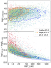 |
Fig. 15 Rest-frame 0.5–2 keV intrinsic luminosity Lx (upper panel) and its 1-σ confidence interval width (lower panel) as a function of the 0.2–2.3 keV source detection likelihood for the AGN with good red-shifts. Sources with posterior median logNH below 20.5, between 20.5 and 21.5, and above 21.5 are plotted in blue, green, and red, respectively. The contours indicate 68% of the sample in the three cases. For representation purposes, we only plot randomly-selected half of the sources. |
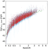 |
Fig. 16 Rest-frame 0.5–2 keV intrinsic luminosity Lx and redshift (in the scale of log(l + z)) distribution of the AGN with good redshift measurements (zG ⩾ 3) and with spectral measurements of Lx (LxModel 1,3,or 4). The median and the 68% percentile interval measured from the posterior Lx distributions are plotted with red points and light-blue error bars. The green line is the 90%-detection curve of AGN with logNH < 21 measured through simulation (Liu et al. 2022b). For representation purposes, we only plot randomly-selected half of the sources. |
4.6 X-ray–UV correlations
Paper II has measured photo-z of all the eFEDS sources through SED fitting. Based on the multiband photometry data and the best-fit SED model, we measure the UV 2500 Å and optical 5100 Å rest-frame monochromatic luminosities L2500 and L5100. For the sources with spec-z, we rerun the SED fitting with the redshift fixed at the spec-z. We use the photometry data between rest-frame 1500 Å and 3500 Å to measure L2500 and the data between rest-frame 4100 Å and 6100 Å to measure L5100. In these two bands, we normalize the best-fit SED component of AGN plus host galaxy to the data separately, multiplying the model by the mean data to model ratio f2500 and f5100 to calculate L2500 and L5100, respectively. We do not decompose the AGN and the host galaxy components, only a separate stellar component, if detected in the SED, is excluded from the luminosity measurements. We consider the L2500 and L5100 as good measurements only if the data quality satisfies the following criteria. First, the source must have either spec-z or the highest-quality photo-z (zG = 4). We require at least three photometry data points in the 1500 Å-3500 Å band, thus excluding the low-redshift sources. For L5100, which is in the optical band where most sources have relatively better photometry, we require at least one data point in the 4100 Å–6100 Å band. We require the mean data-to-model ratios in these two bands f2500 and f5100 in the range of 0.7–1.4 (0.15 dex). When the data to model deviation exceeds this range, we consider the SED model as less reliable. These criteria result in 10655 L2500 measurements and 12714 L5100 measurements.
The distributions of L2500 and L5100 are displayed in Fig. 17. Discontinuity and bimodality can be seen in the luminosities-redshift distributions, which reflect various sample selection effects in the hybrid multiband redshift catalog and various SED models adopted in the photo-z measurements. At high L2500, the sources show a strong correlation between L2500 and L5100, indicating they are typical type-I AGN with a blue UV-optical continuum. At low L2500, the L5100 becomes higher than L2500, suggesting strong UV extinction in type-II AGN and/or strong contamination from host galaxies. We use a criterion of L5100–L2500 < 0.2 to select a subsample of blue AGN. The others are called red AGN.
To analyze the correlation between the X-ray and UV emission, we select only the sources with spectral measurements of LX (model 1, 3, or 4). We select X-ray obscured sources as the well-measured or mildly-measured sources with median logNH ⩾21.5 and select X-ray unobscured sources as the ones with median logNH <21.5 excluding any sources classified as uninformative. Figure 18 displays the correlation between the 0.5–2 keV X-ray luminosity LX and the UV luminosity L2500 for the X-ray unobscured and X-ray obscured sources separately. Since LX is corrected for absorption, both the X-ray unobscured and obscured blue AGN show a strong L5100–L2500 correlation. For red AGN, the L2500 is relatively lower at low luminosities, indicating UV extinction in such sources. This trend of lower L2500 to LX ratio is more significant in the X-ray obscured red AGN, indicating a larger fraction of type-II AGN among such sources.
Figure 19 displays the αOX of the blue AGN, which is defined as

where L2keV, L2500, v2keV, and v2500 are the monochromatic luminosities and frequencies at 2 keV and 2500 Å, respectively. We consider the X-ray unobscured blue AGN as type-I AGN. By linear regression on them, we find the following relation (upper panel of Fig. 19):

The X-ray obscured blue AGN show slightly larger αox than the X-ray unobscured blue AGN, possibly because of selection bias against low-LX obscured AGN. For comparison, we also plot the αox–L2500 relations measured from the ROSAT and XMM-Newton detected SDSS-IV/SPIDERS (Spectroscopic IDentification of eROSITA Sources) type-I AGN catalog (Coffey et al. 2019) and the XMM-COSMOS type-I AGN catalog (Lusso et al. 2010). The differences between these relations might be caused by differences in the intrinsic properties of the AGN, for instance, the black hole mass and accretion rate.
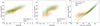 |
Fig. 17 Left and middle panels: L2500–z and L5100–z distributions. Right panel: L2500–L5100 correlation of the sources with both good L2500 and L5100 measurements. Only the sources with spec-z (green) or with the highest-quality photo-z (zG = 4; orange) are included. |
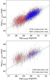 |
Fig. 18 X-ray 0.5–2 keV luminosity vs UV 2500 Åluminosity scatter plots for the X-ray unobscured AGN (upper panel) and X-ray obscured AGN (lower), respectively. UV-strong AGN and UV-weak AGN (with L5100–L2500 below and above 0.2) are plotted in blue and red, respectively. The green lines are obtained by linear regression among the unobscured, UV-strong AGN (blue points in the upper panel). |
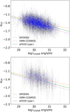 |
Fig. 19 αOX–L2500 scatter plots of the X-ray unobscured (upper panel) and obscured (lower) blue AGN. The green solid line (αOX = 2.840.14 log L2500) is based on the eFEDS type-I subsample (upper panel); the orange dashed line (αOX = 2.39–0.124 log L2500) is measured from the SPIDERS AGN catalog (Coffey et al. 2019); the magenta dash-dotted line (αOX = 3.176–0.154 log L2500) is from the XMM-COSMOS AGN catalog (Lusso et al. 2010). |
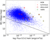 |
Fig. 20 Distribution of the eFEDS AGN in the space of the WISE W1 magnitude versus the observed 0.5–2 keV flux. The 19 luminous AGN are plotted as red points. The red diamonds and green squares indicate the six obscured luminous AGN and the seven radio-detected ones, respectively. The black line corresponds to W1 = –1.625logFlux0.5–2 keV-8.8 (Salvato et al. 2018). |
4.7 Particular AGN
Among the 81 AGN in our catalog with 0.5–2 keV intrinsic luminosities (LumiIntr_Med_s) above 1046 erg/s, there are 19 reliable ones with good redshift measurements (zG ⩾3) and spectral measurements of X-ray luminosities (model 1, 3, or 4). Out of them, only five have the best-quality redshifts (zG ⩾4), including three spec-z (ID 86, 830, 25176) and two photo-z (ID 2157, 2753), all of which have z > 2.2. There are 10 (out of 19) luminous AGN obscured with median logNH above 21 and five above 22 (ID 505, 4944, 21377, 21558, 25176). We look for radio counterparts of these luminous AGN in the 1.4 GHz FIRST survey catalog (White et al. 1997) and the 3 GHz VLASS Epoch 1 catalog (Gordon et al. 2020), adopting a searching radius of 2”. Seven sources (ID 19, 86, 830, 2157, 2267, 505, 4005) are detected in the VLASS catalog, and the first five of them are also detected in the FIRST catalog. In Fig. 20, we compare these luminous AGN with others in the space of infrared magnitude and X-ray flux. A few of them have abnormally large X-ray to infrared flux ratios, especially the radio-detected ones, indicating existence of powerful or even beamed jets.
We noticed that a type-I AGN 2MASX J09325962+0405062 (ID = 352, z = 0.0592) has an extremely flat power-law slope of 1.33 (1.16 ~ 1.51). Its flat spectral shape might be due to Compton-thick absorption or due to a warm absorber. To test the type-I Compton-thick scenario, we performed simultaneous optical and X-ray spectroscopic observations. We observed this source with Chandra on Jan 26 and 28, with a total exposure time of 50 ks. We performed optical photometry on Jan 10, 11, 13, 16, 18, 26, 27, 28, and 29 with the GROND instrument on the 2.2m ESO/MPG telescope and optical spectroscopy on Jan 24, 26, 27, and 29 at Asiago. The optical observations confirmed the type-I AGN nature of this source at the time of the Chandra observation. However, the Chandra spectrum can be well described by a powerlaw with a photon index of 1.63 ± 0.09 and does not require a Compton-thick absorption model or a warm absorber. Therefore, this source is more of a typical type-I AGN. The flat slope measured by eROSITA might be caused by spectral variability.
5 Conclusion
We present the AGN catalog (22 079 sources) selected from the eFEDS main X-ray catalog (27910 sources). To investigate the X-ray spectral properties of AGN, we extract and analyze the spectra of all the eFEDS sources, assuming all of them are point sources. As the first systematical analysis of eROSITA AGN spectra, we describe in detail the point-source spectra extraction methodology of eROSITA in the scanning mode. Using a Bayesian method, we fit the spectra of all the sources, with a second aim of exploring the lower limit of spectral constraining capability of eROSITA. We adopt a single-temperature plasma model for stars and a few power-law-based models for AGN. As simplified versions of the power-law model, we fix the power-law slope parameter at 2.0 and even fix the AGN absorption NH at 0, and limit the fitting to narrow soft or hard band instead of the broad band. As enriched versions, we add a soft power-law or a soft blackbody component to the primary power-law to model the potential soft excess component. With both these two phenomenological soft excess models, we can describe well the broad-band spectral shape of the eFEDS AGN because of their limited S/N. For the sake of information completeness, the spectral fitting results of all the models are presented together with the AGN catalog, as summarized in Table 1.
In the AGN catalog, we choose the most appropriate models to present different aspects of the AGN properties, including spectral shape parameters, soft and hard band fluxes, and soft-band intrinsic luminosities. We use the single-powerlaw model (model 1) to measure the AGN obscuring NH and use the powerlaw + blackbody model (model 3) to measure the slopes of the primary power law. The posterior output of Bayesian spectral analysis cannot always be adopted directly without considering the impact of the adopted prior. We introduce a method of quantifying this impact based on Kullback-Leibler divergence and HDI confidence interval. Using this method, we classify the NH measurements as uninformative, unobscured, mildly-measured, or well-measured, and select obscured AGN as the sources with well-measured or mildly-measured NH and having a median logNH >21.5. To suppress the fraction of uninformative sources, whose data quality does not allow any meaningful spectral analysis, we suggest a sample selection threshold of detection likelihood > 10. To cope with the large and asymmetric parameter uncertainty of each source, we use the HBM method to estimate the parameter distribution of samples. The intrinsic NH distribution of this catalog inferred using the HBM method is largely dominated by unobscured sources and has a 8% fraction of obscured sources with logNH above 21.5. We also use the HBM method to derive a Gaussian distribution for the primary-power-law slope measured by the powerlaw + blackbody model and find a mean of 2.07 and a standard deviation of 0.24. The low obscured fraction and the relatively steep slope reflects the soft-band dominated sample selection bias of eFEDS.
We also present the rest-frame 2500 Å and 5100 Å luminosities, when multiband photometry is available within a ±1000 Å wavelength range. The eFEDS AGN can be divided into two types by applying a threshold to the L2500 to L5100 ratio, i.e., blue AGN that are likely type-I and red AGN that are likely type-II or have strong contamination from host galaxies. The blue AGN show a strong correlation between X-ray and UV emission. The αOX of the blue AGN is anticorrelated with L2500.
Since eROSITA is much more sensitive in the soft band (<2.3 keV) than in the hard band, the eFEDS AGN catalog is more of a soft-X-ray selected catalog and thus is biased for unobscured, steep-slope sources. A detailed study of the less-biased, hard-band selected eFEDS AGN is presented in Nandra et al. (in prep.). More spectroscopic follow-up of eFEDS sources has been done in SDSS-V (Merloni et al., in prep.), a more detailed investigation of the physical properties of the eFEDS AGN based on the optical properties will be presented in a following paper. The upcoming first eROSITA all-sky survey (eRASS1) will be ~300 times larger than eFEDS in area, but eFEDS is deeper than eRASS1 by about an order of magnitude in exposure depth except in the regions near the ecliptic poles. Observed in scanning mode, the sources have averaged PSF, vignetting, and effective area, which are therefore similar between eFEDS and eRASS with a slight difference caused by the different scanning strategies.
Acknowledgements
This work is based on data from eROSITA, the soft X-ray instrument aboard SRG, a joint Russian-German science mission supported by the Russian Space Agency (Roskosmos), in the interests of the Russian Academy of Sciences represented by its Space Research Institute (IKI), and the Deutsches Zentrum für Luft- und Raumfahrt (DLR). The SRG spacecraft was built by Lav-ochkin Association (NPOL) and its subcontractors, and is operated by NPOL with support from the Max Planck Institute for Extraterrestrial Physics (MPE). The development and construction of the eROSITA X-ray instrument was led by MPE, with contributions from the Dr. Karl Remeis Observatory Bamberg and ECAP (FAU Erlangen-Nuernberg), the University of Hamburg Observatory, the Leibniz Institute for Astrophysics Potsdam (AIP), and the Institute for Astronomy and Astrophysics of the University of Tübingen, with the support of DLR and the Max Planck Society. The Argelander Institute for Astronomy of the University of Bonn and the Ludwig Maximilians Universität Munich also participated in the science preparation for eROSITA. The eROSITA data shown here were processed using the eSASS/NRTA software system developed by the German eROSITA consortium. Funding for the Sloan Digital Sky Survey IV has been provided by the Alfred P. Sloan Foundation, the U.S. Department of Energy Office of Science, and the Participating Institutions. SDSS acknowledges support and resources from the Center for High-Performance Computing at the University of Utah. The SDSS website is www.sdss.org SDSS is managed by the Astrophysical Research Consortium for the Participating Institutions of the SDSS Collaboration including the Brazilian Participation Group, the Carnegie Institution for Science, Carnegie Mellon University, Center for Astrophysics | Harvard and Smithsonian (CfA), the Chilean Participation Group, the French Participation Group, Instituto de Astrofısica de Canarias, The Johns Hopkins University, Kavli Institute for the Physics and Mathematics of the Universe (IPMU) / University of Tokyo, the Korean Participation Group, Lawrence Berkeley National Laboratory, Leibniz Institut für Astrophysik Potsdam (AIP), Max-Planck-Institut für Astronomie (MPIA Heidelberg), Max-Planck-Institut für Astrophysik (MPA Garching), Max-Planck-Institut für Extraterrestrische Physik (MPE), National Astronomical Observatories of China, New Mexico State University, New York University, University of Notre Dame, Observatório Nacional/MCTI, The Ohio State University, Pennsylvania State University, Shanghai Astronomical Observatory, United Kingdom Participation Group, Universidad Nacional Autónoma de México, University of Arizona, University of Colorado Boulder, University of Oxford, University of Portsmouth, University of Utah, University of Virginia, University of Washington, University of Wisconsin, Vanderbilt University, and Yale University. The Hyper Suprime-Cam (HSC) collaboration includes the astronomical communities of Japan and Taiwan, and Princeton University. The HSC instrumentation and software were developed by the National Astronomical Observatory of Japan (NAOJ), the Kavli Institute for the Physics and Mathematics of the Universe (Kavli IPMU), the University of Tokyo, the High Energy Accelerator Research Organization (KEK), the Academia Sinica Institute for Astronomy and Astrophysics in Taiwan (ASIAA), and Princeton University. Funding was contributed by the FIRST program from Japanese Cabinet Office, the Ministry of Education, Culture, Sports, Science and Technology (MEXT), the Japan Society for the Promotion of Science (JSPS), Japan Science and Technology Agency (JST), the Toray Science Foundation, NAOJ, Kavli IPMU, KEK, ASIAA, and Princeton University. This paper makes use of software developed for the Large Synoptic Survey Telescope. We thank the LSST Project for making their code available as free software at http://dm.lsst.org The Pan-STARRS1 Surveys (PS1) have been made possible through contributions of the Institute for Astronomy, the University of Hawaii, the Pan-STARRS Project Office, the Max-Planck Society and its participating institutes, the Max Planck Institute for Astronomy, Heidelberg and the Max Planck Institute for Extraterrestrial Physics, Garching, The Johns Hopkins University, Durham University, the University of Edinburgh, Queen's University Belfast, the Harvard-Smithsonian Center for Astrophysics, the Las Cumbres Observatory Global Telescope Network Incorporated, the National Central University of Taiwan, the Space Telescope Science Institute, the National Aeronautics and Space Administration under Grant No. NNX08AR22G issued through the Planetary Science Division of the NASA Science Mission Directorate, the National Science Foundation under Grant No. AST-1238877, the University of Maryland, and Eotvos Lorand University (ELTE) and the Los Alamos National Laboratory. Based [in part] on data collected at the Subaru Telescope and retrieved from the HSC data archive system, which is operated by Subaru Telescope and Astronomy Data Center at National Astronomical Observatory of Japan. M.K. acknowledges support by DFG grant KR 3338/4-1. K.I. acknowledges support by the Spanish MICINN under grant PID2019-105510GB-C33/AEI/10.13039/501100011033.
Appendix A Spectral vs imaging flux
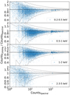 |
Fig. A1 Comparison between the catalog source counts (ML_CTS) and the net counts measured from the spectra, both of which are corrected for PSF-loss outside the extraction region but not corrected for vignetting. The gray lines indicate the 1σ and 2σ interval expected by the Poisson distribution. |
With the source and background spectra, a net source count can be calculated by subtracting the scaled background signal from the source signal. We correct it for the PSF loss using the average correction values in the corresponding energy range stored in the ARF. Fig. A.1 compares the source counts measured from the spectra and that measured through image fitting in the X-ray catalog in a few bands. Both of them correspond to PSF-corrected, vignetted source counts. The catalog source counts are relatively lower by a few percent. Such a lower count measurement in the catalog was also found by simulation comparing its output counts with its input counts (Liu et al. 2022b). This deviation is likely caused by different PSF models adopted by different eSASS tasks. Both the simulation in Liu et al. (2022b) and the spectra extraction in this work use the 2D PSF model (Dennerl et al. 2020), and the count rate measurement in both the real and mock catalogs uses the shapelet PSF model (Paper I).
Assuming a power-law with a slope of 2.0 and with Galactic NH =3×1020 cm−2, the energy conversion factor (ECF) from the 0.2–2.3 keV count rate to the 0.5–2 keV observed flux is 1.557×1012 cm2/erg. With this ECF, we convert the 0.2–2.3 keV count rate from the eFEDS catalog into 0.5–2 keV flux. Fig. A.2 compares this count-rate-based flux and the spectral flux measured using the shape-fixed-powerlaw model for the faint sources with less than 10 net counts in the 0.2–5 keV band. They are measured from the same data (both in the 0.2–2.3 keV band) assuming the same spectral model. However, the count rate is measured through maximum-likelihood PSF-fitting to the image using C-statistic and the spectral flux is measured using a Bayesian method. We find that the count rate measured by the maximum-likelihood fitting tends to truncate near the sensitivity limit; their uncertainties are also truncated accordingly at certain values. This is a numerical bias. It can be avoided by the Bayesian method, which allows the measurement to naturally spread over a wide rage.
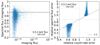 |
Fig. A2 Comparison between 0.5–2 keV fluxes measured from the 0.2–2.3 keV spectral fitting and from the 0.2–2.3 keV count rate (imaging) for sources with less than 10 net counts in the 0.2–5 keV band. The relative errors in the right panel are the ratio between the 1-σ upper and lower limits and the median value, thus the upper and lower limits are displayed in the ranges > 1 and < 1, respectively. |
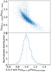 |
Fig. A3 Ratio between the 0.5–2 keV fluxes measured using the powerlaw + blackbody model and using the shape-fixed-powerlaw model (lower panel), and its correlation with the spectral softness, i.e., the ratio between the 0.5–1 keV and 1–2 keV fluxes measured using the power-law + blackbody model. |
It is common to adopt a fixed spectral shape to convert count rates to fluxes in X-ray catalogs (e.g., Paper I). For high-quality spectra, a spectral fit that properly models the spectral shapes and features gives rise to a more accurate flux measurement. As displayed in Fig. A.3, the ratio between the 0.5–2 keV fluxes measured using the powerlaw + blackbody model and that using the shape-fixed-powerlaw model has a median of 1.00 and a standard deviation of 0.11, and the ratio shows a strong correlation with the spectral softness, i.e., the ratio between the 0.5–1 keV and 1–2 keV fluxes measured using the powerlaw + blackbody model. The consistency indicates that the Γ = 2 spectral shape is a good assumption in the ECF calculation of the eFEDS catalog (Paper I). The scatter and the correlation reveal the additional flux uncertainty caused by spectral shape variety, which is not considered when calculating fluxes using a single ECF value.
Appendix B Catalog content description
As listed in Table. 1, we present the eFEDS AGN catalog and the X-ray spectral properties of all the eFEDS sources. The eFEDS AGN catalog provides the AGN NH measured with the single-powerlaw model, the power-law slopes measured with the powerlaw + blackbody model, and the fluxes/luminosities based on the most appropriate models selected in § 3.5 and § 4.5. The columns of this catalog are described in Table. B.1.
Columns of the eFEDS AGN catalog
In the second table as listed in Table. 1, we present the basic properties of the X-ray spectra for all the eFEDS sources, including the spectra extraction information and the source count rates and observed fluxes measured from the spectra. The columns of this table are described in Table. B.2.
We also present eight sets of spectral fitting results with different spectral models and settings, i.e., the tables 3~10 listed in Table. 1. The spectral fitting results in these tables are named in a uniform way as described in Table. B.3, although some columns only apply to particular models. For any parameter of the spectral models or any value (e.g., flux and luminosity) derived from the spectral models, we measure a few statistical quantities of its posterior distribution, including the median, the mean, the standard deviation, the 1-σ/2-σ percentile confidence intervals, and the HDI intervals. The values corresponding to the best-fit model are also presented, although we recommend using the above quantities obtained through Bayesian inference. For spectral shape parameters, which are of more interests than normalization parameters, the KL divergence between the prior and posterior distributions is also provided. In the observed-frame 0.5–2 and 2.3–5 keV bands, we provide measurements of both observed and absorption-corrected fluxes. We also present the absorption-corrected fluxes and luminosities in the rest-frame 0.5–2 keV band and at the monochromatic energy 2 keV.
References
- Ahumada, R., Prieto, C. A., Almeida, A., et al. 2020, ApJS, 249, 3 [Google Scholar]
- Aihara, H., Arimoto, N., Armstrong, R., et al. 2018, PASJ, 70, S4 [NASA ADS] [Google Scholar]
- Aihara, H., AlSayyad, Y., Ando, M., et al. 2019, PASJ, 71, 114 [Google Scholar]
- Akaike, H. 1974, IEEE Trans. Automatic Control, 19, 716 [CrossRef] [Google Scholar]
- Arcodia, R., Campana, S., Salvaterra, R., & Ghisellini, G. 2018, A&A, 616, A170 [NASA ADS] [CrossRef] [EDP Sciences] [Google Scholar]
- Arnaud, K. A. 1996, in Astronomical Society of the Pacific Conference Series, 101, Astronomical Data Analysis Software and Systems V, eds. G. H. Jacoby, & J. Barnes, 17 [NASA ADS] [Google Scholar]
- Baronchelli, L., Nandra, K., & Buchner, J. 2020, MNRAS, 498, 5284 [NASA ADS] [CrossRef] [Google Scholar]
- Bianchi, S., Guainazzi, M., Matt, G., Fonseca Bonilla, N., & Ponti, G. 2009, A&A, 495, 421 [NASA ADS] [CrossRef] [EDP Sciences] [Google Scholar]
- Blanton, M. R., Bershady, M. A., Abolfathi, B., et al. 2017, AJ, 154, 28 [Google Scholar]
- Boller, T., Liu, T., Weber, P., et al. 2021, A&A, 647, A6 [EDP Sciences] [Google Scholar]
- Brandt, W. N., & Alexander, D. M. 2015, A&Ar, 23, 1 [NASA ADS] [CrossRef] [Google Scholar]
- Brunner, H., Liu, T., Lamer, G., et al. 2022, A&A, 661, A1 (eROSITA EDR SI) [NASA ADS] [CrossRef] [EDP Sciences] [Google Scholar]
- Buchner, J. 2016, Stat. Comput., 26, 383 [Google Scholar]
- Buchner, J. 2019, PASP, 131, 108005 [Google Scholar]
- Buchner, J. 2021, J. Open Source Softw., 6, 3045 [NASA ADS] [CrossRef] [Google Scholar]
- Buchner, J. 2021, J. Open Source Softw., 6, 3001 [CrossRef] [Google Scholar]
- Buchner, J., Georgakakis, A., Nandra, K., et al. 2014, A&A, 564, A125 [NASA ADS] [CrossRef] [EDP Sciences] [Google Scholar]
- Cash, W. 1979, ApJ, 228, 939 [Google Scholar]
- Coffey, D., Salvato, M., Merloni, A., et al. 2019, A&A, 625, A123 [NASA ADS] [CrossRef] [EDP Sciences] [Google Scholar]
- Comparat, J., Merloni, A., Dwelly, T., et al. 2020, A&A, 636, A97 [NASA ADS] [CrossRef] [EDP Sciences] [Google Scholar]
- Crummy, J., Fabian, A. C., Gallo, L., & Ross, R. R. 2006, MNRAS, 365, 1067 [Google Scholar]
- Dawson, K. S., Kneib, J.-P., Percival, W. J., et al. 2016, AJ, 151, 44 [Google Scholar]
- Dey, A., Schlegel, D. J., Lang, D., et al. 2021, AJ, 157, 168 [Google Scholar]
- Dennerl, K., Andritschke, R., Bräuninger, H., et al. 2020, in Society of Photo-Optical Instrumentation Engineers (SPIE) Conference Series, 11444, 114444Q [NASA ADS] [Google Scholar]
- Dwelly, T., Salvato, M., Merloni, A., et al. 2017, MNRAS, 469, 1065 [Google Scholar]
- Foreman-Mackey, D. 2016, J. Open Source Softw., 1, 24 [Google Scholar]
- Freyberg, M., Perinati, E., Pacaud, F., et al. 2020, in Society of Photo-Optical Instrumentation Engineers (SPIE) Conference Series, 11444, 114441O [NASA ADS] [Google Scholar]
- Gaia Collaboration (Brown, A. G. A. et al.) 2021, A&A, 649, A1 [NASA ADS] [CrossRef] [EDP Sciences] [Google Scholar]
- Gierliński, M., & Done, C. 2004, MNRAS, 349, L7 [Google Scholar]
- Gordon, Y. A., Boyce, M. M., O’Dea, C. P., et al. 2020, RNAAS, 4, 175 [NASA ADS] [Google Scholar]
- Gunn, J. E., Siegmund, W. A., Mannery, E. J., et al. 2006, AJ, 131, 2332 [NASA ADS] [CrossRef] [Google Scholar]
- HI4PI Collaboration (Ben Bekhti, N., et al.) 2016, A&A, 594, A116 [NASA ADS] [CrossRef] [EDP Sciences] [Google Scholar]
- Lang, D. 2014, AJ, 147, 108 [Google Scholar]
- Liu, T., Tozzi, P., Wang, J.-X., et al. 2017, ApJS, 232, 8 [NASA ADS] [CrossRef] [Google Scholar]
- Liu, A., Bulbul, E., Ghirardini, V., et al. 2022a, A&A, 661, A2 (eROSITA EDR SI) [NASA ADS] [CrossRef] [EDP Sciences] [Google Scholar]
- Liu, T., Merloni, A., Comparat, J., et al. 2022b, A&A, 661, A27 (eROSITA EDR SI) [NASA ADS] [CrossRef] [EDP Sciences] [Google Scholar]
- Luo, B., Brandt, W. N., Xue, Y. Q., et al. 2017, ApJS, 228, 2 [Google Scholar]
- Lusso, E., Comastri, A., Vignali, C., et al. 2010, A&A, 512, A34 [NASA ADS] [CrossRef] [EDP Sciences] [Google Scholar]
- Miyazaki, S., Komiyama, Y., Kawanomoto, S., et al. 2018, PASJ, 70, S1 [NASA ADS] [Google Scholar]
- Nandra, K., & Pounds, K. A. 1994, MNRAS, 268, 405 [Google Scholar]
- Pierre, M., Pacaud, F., Adami, C., et al. 2016, A&A, 592, A1 [NASA ADS] [CrossRef] [EDP Sciences] [Google Scholar]
- Predehl, P., Andritschke, R., Arefiev, V., et al. 2021, A&A, 647, A1 [EDP Sciences] [Google Scholar]
- Ricci, C., Trakhtenbrot, B., Koss, M. J., et al. 2017, ApJS, 233, 17 [Google Scholar]
- Salvato, M., Buchner, J., Budavári, T., et al. 2018, MNRAS, 473, 4937 [Google Scholar]
- Salvato, M., Wolf, J., Dwelly, T., et al. 2022, A&A, 661, A3 (eROSITA EDR SI) [NASA ADS] [CrossRef] [EDP Sciences] [Google Scholar]
- Schlegel, D. J., Finkbeiner, D. P., & Davis, M. 1998, ApJ, 500, 525 [Google Scholar]
- Simmonds, C., Buchner, J., Salvato, M., Hsu, L. T., & Bauer, F. E. 2018, A&A, 618, A66 [NASA ADS] [CrossRef] [EDP Sciences] [Google Scholar]
- Smee, S. A., Gunn, J. E., Uomoto, A., et al. 2013, AJ, 146, 32 [Google Scholar]
- Smith, R. K., Brickhouse, N. S., Liedahl, D. A., & Raymond, J. C. 2001, ApJ, 556, L91 [Google Scholar]
- Sunyaev, R., Arefiev, V., Babyshkin, V., et al. 2021, A&A, 656, A132 [NASA ADS] [CrossRef] [EDP Sciences] [Google Scholar]
- Toba, Y., Liu, T., Urrutia, T., et al. 2022, A&A, 661, A15 (eROSITA EDR SI) [NASA ADS] [CrossRef] [EDP Sciences] [Google Scholar]
- Verner, D. A., Ferland, G. J., Korista, K. T., & Yakovlev, D. G. 1996, ApJ, 465, 487 [Google Scholar]
- Walter, R., & Fink, H. H. 1993, A&A, 274, 105 [NASA ADS] [Google Scholar]
- White, R. L., Becker, R. H., Helfand, D. J., & Gregg, M. D. 1997, ApJ, 475, 479 [Google Scholar]
- Willingale, R., Starling, R. L. C., Beardmore, A. P., Tanvir, N. R., & O’Brien, P. T. 2013, MNRAS, 431, 394 [Google Scholar]
- Wilms, J., Allen, A., & McCray, R. 2000, ApJ, 542, 914 [Google Scholar]
All Tables
All Figures
|
Fig. 1 Number of X-ray sources (upper panel) and fractions of sources (lower) resulted from counterpart quality and redshift quality selections. The red and blue lines indicate counterpart quality ⩾2 and ⩾3. respectively. The solid and dashed lines indicate good (zG ⩾3) and best (zG ⩾4) redshift measurements, respectively. The thick and thin lines indicate sources in the eFEDS 90%-area region and the KiDS region, respectively. |
| In the text | |
|
Fig. 2 Stacked filled histograms: redshift distributions of the eFEDS AGN with spec-z (5287; zG = 5; in blue), with best photo-z (9643; zG = 4; in green), and with good photo-z (6057; zG = 3; in yellow), respectively. The other AGN (1092; zG <3) are displayed in the magenta empty histogram. For sources with photo-z, the redshift PDF is used in plotting. For comparison, we plot the Gaussian distributions centered at z = 1.0 (green dotted line) and z = 1.1 (orange dotted line), which are normalized to the number of AGN with best redshift measurements (zG ⩾4) and good measurements (zG ⩾3), respectively. Both of them have σ = 0.15 in the space of log(l + z). |
| In the text | |
|
Fig. 3 Example of a background extraction region overlaid on the 0.2–2.3 keV image. For source 1702 (at the center), the background extraction region is defined by the area contained between the white annuli, after excluding nearby sources (circles with red stripes). The green and yellow circles indicate point- and extended sources, respectively. Physical scales are printed for the annuli and a source in terms of radii. |
| In the text | |
|
Fig. 4 Distributions of source (blue) and background (orange) extraction radii (upper panel) and distributions of source net counts and background counts in the 0.2–5 keV band (lower panel). The median values of the whole sample are marked with dotted vertical lines. The two-level shaded regions indicate the subsamples of the sources with source net counts ⩾10 and ⩾30, respectively. |
| In the text | |
|
Fig. 5 Background model normalized to a mean value of 1. The red line displays the median of the models of all the sources, and the three-level green shaded regions indicate the 1,2, and 3 σ percentiles. The lower panel displays the ratio to the median. |
| In the text | |
|
Fig. 6 Examples: posterior parameter distributions and spectra (inlaid at upper right) for an AGN (ID = 34) fitted with an absorbed power-law (left) and for a star (ID = 50) fitted with an APEC model (right). The posterior distribution of each individual parameter and each pair of parameters are plotted using the “corner” package (Foreman-Mackey 2016), with the median and 68% percentile interval around the median printed on top of each individual distribution. The spectral shape parameters for the absorbed power-law model include the slope (Γ) of the power-law and the logNH of the intrinsic absorber (in cm–2). For the APEC model, the spectral shape parameters include the Galactic absorption column density logNH, the temperature log KT (in ke V), and the abundance. All the normalization parameters (e.g., logPowNorm, logApecNorm) are measured in logarithm space. The background normalization parameter (logBkgNorm) is set free in the fitting and always equals one. In the spectral plot, the data (dark blue points) are rebinned just for representation to reach an S/N of 3 but allowing at most 6 adjacent bins (each bin includes 4 channels) to be grouped. The blue solid, dashed, and dot-dashed lines display the best-fit model folded with the instrument responses, the folded best-fit source model, and the best-fit background model rescaled to the source extraction region. The shaded region indicates the 99% percentile confidence interval of the model around the median. The lower panel compares the data with the best-fit model in terms of (data-model)/error, where the error is calculated as the square root of the model predicted number of counts. |
| In the text | |
|
Fig. 7 Same as Fig. 6, but for an AGN (ID = 7) fitted with the “double-powerlaw” model (left) and the “powerlaw + blackbody” model (right), respectively. In addition to the power-law normalization (logPowNorm) and the background normalization (logBkgNorm), for the first model, the spectral shape parameters include the ∆Γ for the additional power-law, the Γ of the primary power-law, the logNH, and the flux ratio of the secondary to the primary power-law at 1 keV (logFrac); and for the second model, the parameters determining the spectral shape include the Γ of the power-law, the logNH, the log kT of the blackbody, and the blackbody normalization (logBBNorm). |
| In the text | |
|
Fig. 8 Model comparison on the basis of Δ log Z between pairs of models, i.e., 1) the single-powerlaw (pw) model vs the APEC model; 2) the double-powerlaw (pw+pw) model vs the single-powerlaw model; 3) the powerlaw + blackbody (pw+bb) model vs the single-powerlaw model; 4) the powerlaw + blackbody model vs the double-powerlaw model. The empty histogram indicates all the sources and the filled histogram corresponds to the subsamples of bright sources with at least 20 net counts in 0.2–5 keV band. In the first panel, the blue and orange colors indicate AGN and stars respectively. In the second and third panels, the red color indicates the subsamples of AGN with a median logNH above 21.5. In the last panel, the blue and magenta colors indicate sources with log Zapec − log ZpW below and above 1.3 respectively. |
| In the text | |
|
Fig. 9 Distributions of the posterior median and 1-σ HDI interval as a function of KL divergence for NH (panels N1~N3) and for power-law slope Γ (G1~G3), respectively, as measured using the single-powerlaw model. Examples of source posterior PDF are compared with the prior PDF for NH (N4) and for Γ (G4). The distributions of posterior median values are also displayed for NH (N5) and Γ (G5), respectively. The HDI intervals are plotted as blue error bars for the sources with at least 30 net counts and yellow error bars for the other faint sources. For representation, we only plot the yellow error bars for a random 10% of these faint sources. In panels N1~N3, the AGN catalog is plotted separately in three groups, i.e., N1: sources with the HDI lower limit truncated by the boundary (<19.8); N2 and N3: other sources with the HDI lower limit below and above the green line, which corresponds to logNH = 20.2–2 log KLNH. In panels G1~G3, the catalog is also divided into three, i.e., sources with HDI interval width >0.8 (G1), between 0.55 and 0.8 (G2), and <0.55 (G3). The purple arrowed lines indicate 68% of the NH parameter range at one side of the boundary (N1) or at the center of the range (N2, N3). The magenta arrowed lines indicate the 68% range of the Gaussian(2.0,0.5) prior for Γ. In panels N5 and G5, the blue empty histograms indicate the whole AGN sample; the cyan, green, orange, and red colors indicate the four classes of NH measurements, i.e., 1) uninformative, 2) unobscured, 3) mildly-measured, and 4) well-measured; the purple and magenta colors indicate sources with KLΓ above and below 0.3. In panels N4 and G4, the black lines indicate the prior PDFs; the IDs of example sources for NH PDF are 878 (cyan), 4526 (green), 20 (orange), and 7274 (red); the ID of example sources for Γ PDF are 864 (magenta), 13651 (purple, dashed), 595 (purple, dotted), and 471 (purple, solid). |
| In the text | |
|
Fig. 10 Fractions of sources selected by X-ray spectral properties among the AGN detected in the eFEDS 90%-area region as a function of the 0.2–2.3 keV source detection likelihood. In the upper panel, concerning the NH measurement with the single-powerlaw model, the AGN are divided into four classes, i.e., 1) uninformative (cyan), 2) unobscured (green), 3) mildly-measured (orange), and 4) well-measured (red). In the lower panel, the purple lines indicate the AGN with spectral measurements of LX (discussed in Sect. 4.5), and the solid, dashed, and dash-dotted line styles indicated all the AGN, the AGN with good red-shift measurements, and the AGN with the best redshift measurements, respectively. |
| In the text | |
|
Fig. 11 Upper panel: NH distribution of the eFEDS AGN with good redshifts (zG ⩾3). The stacked filled histograms display the median NH distributions of the AGN with 0.2–5 keV net counts >200 (196 sources; yellow), >20 (6181; yellow and green), and >0 (20987; yellow, green, and blue). The red empty histogram displays the median NH of the sources with well-measured NH (NHclass = 4). The blue and green empty histograms (with 1-σ errorbars) present the inferred intrinsic NH distribution using the HBM method for all the AGN with good redshifts (20987) and the subsample with at least 20 counts (6181), respectively. Lower panel: detected fraction measured by simulation as a function of NH for three subsamples of AGN with 2–10 keV intrinsic luminosity Lx above given logarithmic thresholds and redshift below given thresholds. The three Lx thresholds are selected such that the three subsamples have similar detected fractions at the lowest NH. |
| In the text | |
|
Fig. 12 Comparison between the posterior median power-law slopes measured using the single-powerlaw (pw) model and the powerlaw + blackbody (pw + bb) model for all the AGN with good redshifts. The sources with logZpw+bb–logZpw below 0.5, between 0.5 and 1, and above 1 are plotted in blue, orange, and red, respectively. |
| In the text | |
|
Fig. 13 Distributions of the blackbody temperature and NH measured by the powerlaw + blackbody model for the AGN with soft excess identified through the powerlaw + blackbody model (pw+bb; blue) and the double-powerlaw model (pw+pw; orange), respectively. |
| In the text | |
|
Fig. 14 Upper panel: distributions of the soft-excess relative strength measured by the powerlaw + blackbody model (blue) and the double-powerlaw model (orange), respectively, for the AGN with good redshifts and at least 20 net counts. The values are clipped at a lower limit of 10−6. The blue filled histograms indicate an unobscured subsample with the NH measured by the powerlaw + blackbody model below 1020.5 cm−2. Lower panel: ratio between the slopes of the primary power-law measured by the two models for the unobscured subsample as a function of the blackbody relative strength. The green horizontal line indicates the median value (1.04) of the ratio. |
| In the text | |
|
Fig. 15 Rest-frame 0.5–2 keV intrinsic luminosity Lx (upper panel) and its 1-σ confidence interval width (lower panel) as a function of the 0.2–2.3 keV source detection likelihood for the AGN with good red-shifts. Sources with posterior median logNH below 20.5, between 20.5 and 21.5, and above 21.5 are plotted in blue, green, and red, respectively. The contours indicate 68% of the sample in the three cases. For representation purposes, we only plot randomly-selected half of the sources. |
| In the text | |
|
Fig. 16 Rest-frame 0.5–2 keV intrinsic luminosity Lx and redshift (in the scale of log(l + z)) distribution of the AGN with good redshift measurements (zG ⩾ 3) and with spectral measurements of Lx (LxModel 1,3,or 4). The median and the 68% percentile interval measured from the posterior Lx distributions are plotted with red points and light-blue error bars. The green line is the 90%-detection curve of AGN with logNH < 21 measured through simulation (Liu et al. 2022b). For representation purposes, we only plot randomly-selected half of the sources. |
| In the text | |
|
Fig. 17 Left and middle panels: L2500–z and L5100–z distributions. Right panel: L2500–L5100 correlation of the sources with both good L2500 and L5100 measurements. Only the sources with spec-z (green) or with the highest-quality photo-z (zG = 4; orange) are included. |
| In the text | |
|
Fig. 18 X-ray 0.5–2 keV luminosity vs UV 2500 Åluminosity scatter plots for the X-ray unobscured AGN (upper panel) and X-ray obscured AGN (lower), respectively. UV-strong AGN and UV-weak AGN (with L5100–L2500 below and above 0.2) are plotted in blue and red, respectively. The green lines are obtained by linear regression among the unobscured, UV-strong AGN (blue points in the upper panel). |
| In the text | |
|
Fig. 19 αOX–L2500 scatter plots of the X-ray unobscured (upper panel) and obscured (lower) blue AGN. The green solid line (αOX = 2.840.14 log L2500) is based on the eFEDS type-I subsample (upper panel); the orange dashed line (αOX = 2.39–0.124 log L2500) is measured from the SPIDERS AGN catalog (Coffey et al. 2019); the magenta dash-dotted line (αOX = 3.176–0.154 log L2500) is from the XMM-COSMOS AGN catalog (Lusso et al. 2010). |
| In the text | |
|
Fig. 20 Distribution of the eFEDS AGN in the space of the WISE W1 magnitude versus the observed 0.5–2 keV flux. The 19 luminous AGN are plotted as red points. The red diamonds and green squares indicate the six obscured luminous AGN and the seven radio-detected ones, respectively. The black line corresponds to W1 = –1.625logFlux0.5–2 keV-8.8 (Salvato et al. 2018). |
| In the text | |
|
Fig. A1 Comparison between the catalog source counts (ML_CTS) and the net counts measured from the spectra, both of which are corrected for PSF-loss outside the extraction region but not corrected for vignetting. The gray lines indicate the 1σ and 2σ interval expected by the Poisson distribution. |
| In the text | |
|
Fig. A2 Comparison between 0.5–2 keV fluxes measured from the 0.2–2.3 keV spectral fitting and from the 0.2–2.3 keV count rate (imaging) for sources with less than 10 net counts in the 0.2–5 keV band. The relative errors in the right panel are the ratio between the 1-σ upper and lower limits and the median value, thus the upper and lower limits are displayed in the ranges > 1 and < 1, respectively. |
| In the text | |
|
Fig. A3 Ratio between the 0.5–2 keV fluxes measured using the powerlaw + blackbody model and using the shape-fixed-powerlaw model (lower panel), and its correlation with the spectral softness, i.e., the ratio between the 0.5–1 keV and 1–2 keV fluxes measured using the power-law + blackbody model. |
| In the text | |
Current usage metrics show cumulative count of Article Views (full-text article views including HTML views, PDF and ePub downloads, according to the available data) and Abstracts Views on Vision4Press platform.
Data correspond to usage on the plateform after 2015. The current usage metrics is available 48-96 hours after online publication and is updated daily on week days.
Initial download of the metrics may take a while.