| Issue |
A&A
Volume 659, March 2022
|
|
|---|---|---|
| Article Number | A173 | |
| Number of page(s) | 37 | |
| Section | Extragalactic astronomy | |
| DOI | https://doi.org/10.1051/0004-6361/202142624 | |
| Published online | 23 March 2022 | |
A 2–3 mm high-resolution molecular line survey towards the centre of the nearby spiral galaxy NGC 6946⋆
1
Argelander-Institut für Astronomie, Universität Bonn, Auf dem Hügel 71, 53121 Bonn, Germany
e-mail: This email address is being protected from spambots. You need JavaScript enabled to view it.
2
Max Planck Institut für Astronomie, Königstuhl 17, 69117 Heidelberg, Germany
3
Max-Planck-Institut für Extraterrestrische Physik, Giessenbachstraße 1, 85748 Garching, Germany
4
New Mexico Institute of Mining and Technology, 801 Leroy Place, Socorro, NM 87801, USA
5
National Radio Astronomy Observatory, PO Box O, 1003 Lopezville Road, Socorro, NM 87801, USA
6
Observatorio Astronómico Nacional (IGN), C/ Alfonso XII 3, 28014 Madrid, Spain
7
Department of Astronomy, The Ohio State University, 4055 McPherson Laboratory, 140 West 18th Avenue, Columbus, OH 43210, USA
8
4-183 CCIS, University of Alberta, Edmonton, Alberta T6G 2E1, Canada
9
Centre for Astrophysics Research, School of Physics, Astronomy and Mathematics, University of Hertfordshire, College Lane, Hatfield AL10 9AB, UK
10
Institut de Radioastronomie Millimétrique (IRAM), 300 Rue de la Piscine, 38406 Saint Martin d’Hères, France
11
LERMA, Observatoire de Paris, PSL Research University, CNRS, Sorbonne Universités, 75014 Paris, France
12
European Southern Observatory, Karl-Schwarzschild Straße 2, 85748 Garching bei München, Germany
13
Univ. Lyon, Univ. Lyon1, ENS de Lyon, CNRS, Centre de Recherche Astrophysique de Lyon UMR5574, 69230 Saint-Genis-Laval, France
14
National Radio Astronomy Observatory (NRAO), 520 Edgemont Road, Charlottesville, VA 22903, USA
15
Astronomisches Rechen-Institut, Zentrum für Astronomie der Universität Heidelberg, Mönchhofstraße 12-14, 69120 Heidelberg, Germany
16
Universität Heidelberg, Zentrum für Astronomie, Institüt für Theoretische Astrophysik, Albert-Ueberle-Strasse 2, 69120 Heidelberg, Germany
17
Department of Astronomy, Xiamen University, Xiamen, Fujian 361005, PR China
18
Purple Mountain Observatory, Chinese Academy of Sciences (CAS), Nanjing 210023, PR China
19
Research School of Astronomy and Astrophysics, Australian National University, Canberra, ACT 2611, Australia
20
Universität Heidelberg, Interdisziplinäres Zentrum für Wissenschaftliches Rechnen, INF 205, 69120 Heidelberg, Germany
21
Department of Physics, Tamkang University, No. 151, Yingzhuan Rd., Tamsui Dist., New Taipei City 251301, Taiwan
22
Center for Astrophysics and Space Sciences, University of California San Diego, 9500 Gilman Drive, La Jolla, CA 92093, USA
Received:
9
November
2021
Accepted:
20
December
2021
Abstract
The complex physical, kinematic, and chemical properties of galaxy centres make them interesting environments to examine with molecular line emission. We present new 2 − 4″ (∼75 − 150 pc at 7.7 Mpc) observations at 2 and 3 mm covering the central 50″ (∼1.9 kpc) of the nearby double-barred spiral galaxy NGC 6946 obtained with the IRAM Plateau de Bure Interferometer. We detect spectral lines from ten molecules: CO, HCN, HCO+, HNC, CS, HC3N, N2H+, C2H, CH3OH, and H2CO. We complemented these with published 1 mm CO observations and 33 GHz continuum observations to explore the star formation rate surface density ΣSFR on 150 pc scales. In this paper, we analyse regions associated with the inner bar of NGC 6946 – the nuclear region (NUC), the northern (NBE), and southern inner bar end (SBE) and we focus on short-spacing corrected bulk (CO) and dense gas tracers (HCN, HCO+, and HNC). We find that HCO+ correlates best with ΣSFR, but the dense gas fraction (fdense) and star formation efficiency of the dense gas (SFEdense) fits show different behaviours than expected from large-scale disc observations. The SBE has a higher ΣSFR, fdense, and shocked gas fraction than the NBE. We examine line ratio diagnostics and find a higher CO(2−1)/CO(1−0) ratio towards NBE than for the NUC. Moreover, comparison with existing extragalactic datasets suggests that using the HCN/HNC ratio to probe kinetic temperatures is not suitable on kiloparsec and sub-kiloparsec scales in extragalactic regions. Lastly, our study shows that the HCO+/HCN ratio might not be a unique indicator to diagnose AGN activity in galaxies.
Key words: galaxies: ISM / ISM: molecules / galaxies: individual: NGC 6946
Based on observations carried out with the IRAM Plateau de Bure Interferometer (PdBI). IRAM is supported by INSU/CNRS (France), MPG (Germany) and IGN (Spain).
© ESO 2022
1. Introduction
The study of star-forming regions within galaxy centres is of particular interest, as the extreme conditions within these regions are thought to greatly influence their host giant molecular cloud (GMC) populations, and, thus, the stellar populations that they may form. For example, the inner few kiloparsecs of galaxies typically have higher average gas and stellar densities, gas temperatures, levels of turbulence and magnetic field strengths relative to their discs. All of these characteristics have direct implications for the physical, dynamical and chemical properties of the star-forming ‘dense’1 molecular gas within systems (see e.g. McKee & Ostriker 2007; Lada et al. 2010, 2012; Longmore et al. 2013; Klessen & Glover 2016).
Molecular gas is denser in centres than is typically inferred within disc star-forming regions; the cause of this are strong compressive tidal forces, frequent molecular cloud interactions, short dynamical timescales, constant feeding of material via, for example, bars (e.g. Schinnerer et al. 2006, 2007), and feedback from both young and old stars (e.g. Kruijssen et al. 2019; Chevance et al. 2020a,b; Barnes et al. 2020a) along with energetic phenomena within the galaxy centres (e.g. AGN; Combes et al. 2013; Querejeta et al. 2016) and this should favour star formation. However, it is seen both within the Milky Way (e.g. Kruijssen et al. 2014; Barnes et al. 2017) and inferred at centres of nearby galaxies (e.g. Gallagher et al. 2018a; Jiménez-Donaire et al. 2019) that the gas over-density required to form stars is also higher. Averaged over the galaxy population (and thereby presumably over episodic variations, e.g. Krumholz et al. 2017), centres show an apparent deficit of star formation despite their large quantities of dense molecular gas (e.g. Bigiel et al. 2015; Usero et al. 2015; Jiménez-Donaire et al. 2019 among others). For a complete understanding of star formation, the study of these complex environments present in galaxy centres is crucial.
Observations and simulations of a Milky Way-like galaxy suggest that large-scale bars (a few kiloparsecs) could be responsible for a molecular gas mass build-up in the central few hundred parsecs (e.g. Díaz-García et al. 2020; Renaud et al. 2015; Emsellem et al. 2015; Sormani & Barnes 2019; Sormani et al. 2020). The overlap between the end of those large-scale bars and the spiral arms are – in addition to the centre – active star-forming regions coupled with enhanced dense gas, for example the bar ends of NGC 3627 (Beuther et al. 2017; Bešlić et al. 2021). Secondary small-scale bars (a few hundred parsecs) of double barred galaxies (e.g. Erwin 2011) were intensively studied through photometric analysis (e.g. Méndez-Abreu et al. 2019; de Lorenzo-Cáceres et al. 2020). However, secondary small-scale bars (we refer to them as ‘inner bar’ in this work) have been hardly observed with emission from multiple rotational molecular line transitions. This leads us to question if we would find also enhanced molecular line emission (indicating increased gas volume densities) and/or star formation activity at the inner bar ends compared to the surrounding environment (i.e. as with larger scale galactic bars). And how does this relate to the increased dense gas fraction (fdense), and yet decreased dense gas star formation efficiency (SFEdense), typically observed in galaxy centres.
The emission from rotational molecular line transitions observed within the radio domain is typically used to study the aforementioned properties of the molecular interstellar medium (ISM). Studies conducted over the past several decades found that emission of high-critical-density tracers, such as Hydrogen Cyanide (HCN), Formylium ion (HCO+), Carbon Monosulfide (CS), and Diazenylium (N2H+) are prevalent across galaxy centres, suggesting the presence of large amounts of ‘dense’ molecular gas (Mauersberger et al. 1989; Mauersberger & Henkel 1989, 1991; Nguyen et al. 1992; Solomon et al. 1992; Helfer & Blitz 1993). More recently, higher angular resolution observations have allowed the study of dense gas content of individual centres of galaxies on sub-kiloparsec scales (e.g. Schinnerer et al. 2007; Pan et al. 2015; Tan et al. 2018 for NGC 6946; Martín et al. 2015 for NGC 253; Murphy et al. 2015 for NGC 3627; Salak et al. 2018 for NGC 1808; Querejeta et al. 2019 for M 51; Bemis & Wilson 2019 for NGC 4038 and NGC 4039; Callanan et al. 2021 for M 83).
Galaxy centres also have a rich and diverse chemistry that could be used to probe the environmental conditions of gas beyond just the density (e.g. Morris & Serabyn 1996; Belloche et al. 2013; Rathborne et al. 2015; Barnes et al. 2019; Petkova et al. 2021 for the Milky Way; Meier & Turner 2005 for IC 342; Meier & Turner 2012 for Maffei 2; Aladro et al. 2013 for NGC 1068; Meier et al. 2015; Leroy et al. 2018; Krieger et al. 2020; Holdship et al. 2021 for NGC 253; Martín et al. 2015 for NGC 1097; Henkel et al. 2018 for NGC 4945). These studies used molecular line ratio diagnostics to investigate the physics and chemistry of the ISM in these extreme environments. But many open questions still remain, such as: how the location of active formation of young massive stars correlate with that of the various molecular line tracers, or, what the ratios between molecular lines indicate about temperature, excitation and density structure in the gas.
NGC 6946 is an ideal candidate to study the effect of large and small scale bars on the dense gas and chemistry through molecular line emission. NGC 6946 has beside its large-scale stellar bar with a length of 100 − 120″ (≈3.7 − 4.5 kpc) (Regan & Vogel 1995; Menéndez-Delmestre et al. 2007; Font et al. 2014), a small-scale bar (see below), and is one of the nearest large double-barred spiral galaxies (D ≈ 7.72 Mpc; see Table 1). It does not seem to host an AGN (see Sect. 6.3) and leads the list of observed supernovae in a nearby galaxy disc (10 supernovae2), which has led to its name Fireworks Galaxy.
Properties of NGC 6946.
In this work, we study the inner 50″ ≈ 1.9 kpc of NGC 6946, which has previously been the target for many multi-wavelength observations which we can use to compare to, and build upon, for our analysis. We use ancillary 33 GHz continuum data (Murphy et al. 2018; Linden et al. 2020) to obtain the SFR from the free-free emission part to compare dense gas, total molecular gas, and extinction-free estimates of recent star formation across the inner star-forming centre of NGC 6946. In the sketch in Fig. 1, we see in green colours three distinct regions in 12CO (2−1) (hereafter CO(2−1)). The appearance of these three features as an S-shaped structure have been explained with modelling efforts in Schinnerer et al. (2006). To do so, they obtained a three-dimensional representation of the luminosity and mass distribution of the galaxy using the multi-Gaussian expansion (MGE) method (see e.g. Emsellem et al. 2003). They then inferred the corresponding axisymmetric gravitational potential by using the Poisson equation and assuming a constant mass-to-light ratio, which is then perturbed by adding a ∼kpc bar-like structure to the MGE potential (as in Emsellem et al. 2003). They showed that their model reproduces the observed (straight) ∼kpc gas lane morphologies, when applying an inner bar with a radius of ∼250 pc (or 6.5 − 8″ projected into the galaxy plane) with a pattern speed Ωp of 510 − 680 km s−1 kpc−1. They concluded that molecular gas flows inwards from the outer disc, shaping and driving the evolution of the centre of NGC 6946. Therefore, we refer to their ‘clumps’ as the bar ends of the inner bar (see green ellipses in the sketch of Fig. 1). This allows us to study different regions in the centre: (a) the nuclear region – NUC, (b) the northern inner bar end – NBE, and (c) the southern inner bar end – SBE, which we refer to as abbreviated above throughout this work.
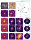 |
Fig. 1. Gallery of the multi-wavelength observation towards the centre of NGC 6946. Left panels: (a) three colour optical image, with the region of interest drawn as a purple box, (b) CO(1−0) emission shown in contours levels of 60, 90, 200, 300, 600 K km−1 s−1, and are repeated on all panels for comparison, (c) integrated CO(1−0) emission, (d) CO(2−1) emission towards the inner 20″ shown as colour scale; sketch (right): denoting all observed features (see Sect. 2.4 for an overview), (e)–(g) continuum emission, (h)–(j) infrared emission and (k)–(m) hydrogen recombination lines and X-ray emission (see Table A.1 for references of all observations shown). The rightmost column shows integrated intensity maps of three of our fourteen detected emission lines for comparison. Optical image credits: NASA, ESA, STScI, R. Gendler, and the Subaru Telescope (NAOJ). |
In this work we present a suite of lines observed across the 1 − 3 mm IRAM Plateau de Bure Interferometer (PdBI) window [PI: E. Schinnerer] to assess the physical and chemical structure of the inner ∼50″ of NGC 6946 (see Fig. 2). This gives us one of the most comprehensive, high resolution (2 − 4″ ≈ 75 − 150 pc) molecular line data set for a nearby galaxy centre in the northern hemisphere. In this first of a series of papers, we present the observations and especially focus on the short-spacing corrected bulk (CO) and dense gas tracers (HCN, HCO+, and HNC).
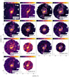 |
Fig. 2. Integrated intensity maps (moment 0) for 14 molecular emission lines at a common resolution of 4″ ≈ 150 pc. The maps were created using a hexagonal sampling with half a beam spacing, where CO(1−0) was used as a mask. The grey shaded circle in the lower left corner marks the beam size and the red contours show CO(1−0) S/N levels of 30, 60 and 90. The white contours in the first panel show S/N levels of 200 and 300, and in the second panel S/N levels of 30, 60 and 90. The following panels (from HCN to H2CO(2 − 1)) show S/N levels of 3, 6, 9, 30, 60 and 90. The colourbar indicates the integrated intensity of each line in units of K km s−1. See Table 1 for the properties of this data set. |
This paper is structured as follows: In Sect. 2, we present how the PdBI observations were taken, calibrated and imaged, along with information of the ancillary observations used within this work and how we convert observational measurements to physical quantities. Section 3 shows the results and Sect. 4 the discussion of our extended data set. In Sect. 5, we show the results from our short-spacing corrected data set focusing on the nuclear region and inner bar ends. In Sect. 6, we discuss line ratio diagnostics of the short-spacing corrected data set and possible implications for spectroscopic studies of other galaxy centres.
2. Observations and ancillary data
2.1. PdBI observations and data reduction
The Plateau de Bure Interferometer (PdBI) was used to image molecular lines at 1.3 to 3 mm using a single pointing focusing on the central 50″ of NGC 6946 for a total of 132 h from 2002 to 2009. Eight high-resolution spectral windows were used in each observation, each offering a bandwidth of 160 MHz and channel width of 2.5 MHz (i.e. 9 km s−1 at 87 GHz). The data, acquired from multiple observations (project codes: Q059, R02C, R09F, S02A, R09F, S08E, P069, M032 and S02A; PI: Schinnerer), were split between five spectral setups at reference frequencies of ∼87 GHz (setup A), ∼97 GHz (setup B), ∼92 GHz (setup C), ∼115 GHz (setup D) and ∼230 GHz (setup one mm). We identified in the spectral setup A: C2H(1 − 0), HCO+(1 − 0) and HCN(1−0), in setup B: CH3OH(2 − 1), CS(2−1), CH3OH(3 − 2), HC3N(16 − 15), H2CO(2 − 1) and CS(3−2), in setup C: HNC(1−0), HC3N(10 − 9) and N2H+(1−0), in setup D: CO(1−0), in setup one mm: CO(2−1) (see Table 2). The primary beam FWHM ranges from ∼57″ at 87 GHz to ∼43″ at 115 GHz and ∼22″ at 230 GHz. The spectral window of each molecular line was centred on the redshifted frequency of the line assuming a systemic velocity of 50 km s−1 for NGC 6946 (Schinnerer et al. 2006). The imaged width in each spectral window is the velocity width at zero level of the CO(1−0) line (300 km s−1, matching the Full Width at Zero Intensity of the HI line seen by THINGS in Walter et al. 2008) plus 50 km s−1 on each side of the line centre. These data were all calibrated and imaged using GILDAS3. For the bandpass calibration, observations of the bright quasars 3C 454.3, 2145+067, 0923+392 and 3C 273 have been used. The phase and amplitude calibrators were either both 2037+511 and 1928+738 or one of them. These calibrators were observed every 20 min. Most of the observations compared MWC 349 observations with its IRAM flux model to calibrate the absolute flux scale. We expect an accuracy of the flux calibration of about 5% at 3 mm and a typical antenna aperture efficiencies of about 25 Jy K−1 at 3 mm, and 28 Jy K−1 at 2 mm data.
Summary of the molecular lines in our compiled data set towards the centre of NGC 6946.
The continuum emission has been combined with the UV MERGE task after excluding the line channels. The spectral lines were resampled to 10 km s−1 for all the lines during the creation of UV tables in the GILDAS CLIC environment. The continuum has been subtracted in the u − v plane with the above continuum u − v table extracted from all line-free channels with the UV SUBSTRACT task before the imaging. Imaging of the visibilities used natural weighting, where each visibility is weighted by the inverse of the noise variance, as this maximises the sensitivity. The field of view of each image is twice the primary beam with pixel sizes 1/4 of the synthesised beam major axis FWHM size (ranging from 0.4″ × 0.29″ to 2.0″ × 1.7″ and 3.6″ × 2.9″, see Table 3).
Properties of the PdBI only data set.
Cleaning was performed with a preconstructed clean mask which has been produced similar to the signal identification methodology used in CPROPS (Rosolowsky & Leroy 2006; Rosolowsky et al. 2021; Leroy et al. 2021) using the high resolution (∼1″) CO(1−0) PdBI data without short-spacing correction (Schinnerer et al. 2006). Following Leroy et al. (2021; for the PHANGS-ALMA survey), the clean mask creation includes the following steps: (a) convolving the CO(1−0) beam from ∼1″ to a coarser resolution of 33″ and smoothing along the spectral axis with a boxcar function with a width of 20 km s−1; (b) selecting peak pixels for each channel which have a S/N of at least 4; (c) expanding each peak down to a S/N of 2; (d) binary-dilating 4 channels along the spectral axis to account for edge effect. This produces a clean mask that covers all possible CO signal regions and ensures that the cleaning of other molecular gas tracers is less affected by noisy, no-signal regions outside the mask. The typical rms per channel observed is ≈2 mJy beam−1.
Before being used in the deconvolution, the clean mask was regridded to match the astrometry of the dirty cube of each line. After imaging and deconvolution we corrected for the primary beam attenuation. We provide the observational characteristics of the PdBI only data in Table 3 (and show the channel maps in Figs. A.3–A.14).
Given that these data have different u − v coverage, we built a homogenised product by imaging only the visibilities that are within the u − v coverage of the CO(1−0) PdBI data, that is 11.5 to 153.8 kλ. We do this to match the spatial scales of the CO data. This has been done using a GILDAS script where we loop through all the visibilities and flag the ones outside the CO(1−0) u − v range by assigning negative weights to them. Then the UV TRIM function was used to discard the flagged data.
Interferometric observations are insensitive to emission with low spatial frequencies due to the lack of the shortest baselines. For the short-spacing correction, we utilise IRAM 30 m observations. We use data of the EMIR Multiline Probe of the ISM Regulating Galaxy Evolution (EMPIRE; Jiménez-Donaire et al. 2019) survey which observed in the 3 − 4 mm regime, in particular, HCN across the whole disc of nine nearby spiral galaxies, among them NGC 6946. For the purpose of short-spacing correction (SSC) we use their 33″ resolution HCN(1−0), HCO+(1 − 0) and HNC(1−0) maps. For the CO(2−1) observations, we use data from the HERA CO-Line Extragalactic Survey (HERACLES) (Leroy et al. 2009). For the remaining PdBI detected molecules we do not find public single-dish data with a significant S/N4, therefore, no SSC was feasible for them.
SSC has been done in GILDAS in its MAPPING environment. Before performing SSC on the data available, we ensured that the 30 m data used the same projection center and spectral grid as the interferometric data, before applying the UVSHORT task. This produces pseudo-visibilities that fill the short-spacings before imaging and deconvolution (see Rodriguez-Fernandez et al. 2008; Pety et al. 2013 for details). We summarise the observational characteristics of the SSC + u − v trim data in Table 4.
Properties of the SSC + u − v trim data set.
In summary, within this work we make use of the following data sets: PdBI only, which includes 14 molecular emission lines, and SSC + u − v trim, which includes five molecular emission lines.
2.2. Integrated intensity maps
As a next step, we converted our PdBI only and SSC + u − v trim data cubes from units of Jy beam−1 to brightness temperature, Tb, measured in Kelvin. Our observations include emission lines from a wavelength range of 1 to 3 mm which results in various spatial resolutions. We convolved our data to a common beam size of 4″ (corresponding to 150 pc at 7.72 Mpc distance) and sampled the integrated intensities onto a hexagonal grid. The grid points are spaced by half a beam size to approximately Nyquist sample the maps. This approach has the advantage that the emission lines can be directly compared.
To improve the signal-to-noise ratio (S/N) we applied a masking routine for the determination of the integrated intensity maps. We used the bright CO(1−0) emission line as a prior for masking and produced two S/N cuts: a low S/N mask (S/N > 2) and a high S/N mask (S/N > 4). Subsequently, the high S/N mask is expanded into connected voxels in the low S/N mask, and the integrated intensity is determined by integrating along the velocity axis for each of the individual sight lines multiplied by the channel width, Δvchan, of 10 km s−1:
 (1)
(1)
The uncertainty is calculated taking the square root of the number of masked channels (nchan) along a line of sight multiplied by the 1σ root mean square (σrms) value of the noise and the channel width:
 (2)
(2)
We calculate σrms over the signal-free part of the spectrum using the astropy (Astropy Collaboration 2013, 2018) function mad_std that calculates the median absolute deviation and scales it by a factor of 1.4826. This factor results from the assumption that the noise follows a Gaussian distribution. We show the integrated intensity maps of the PdBI only data in Fig. 2.
2.3. Ancillary data
We include ancillary data for investigating the central regions of NGC 6946 and analysing the relationship of our detected molecules to star formation rate (SFR) tracers. We also compare NGC 6946 with other galaxy centers. Therefore, we include (1) 33 GHz continuum emission, (2) EMPIRE dense gas observations of eight additional galaxy centres (angular resolution of 33″ ≈ 1 kpc), (3) high resolution resolution dense gas observations of M 51 (∼4″ ≈ 166 pc) and NGC 3627 (∼2″ ≈ 100 pc), and (4) 0.5 − 7.0 keV X-ray observations of NGC 6946.
2.3.1. SFR tracers
Tracers of the number of ionizing photons, specifically free-free radio continuum emission and hydrogen recombination lines, are often regarded as good indicators of massive star formation. The radio continuum emission at low frequencies consists of two components: (1) thermal free-free emission directly related to the production rate of ionizing photons in H II regions and (2) non-thermal emission arising from cosmic ray electrons or positrons which propagate through the magnetised ISM after being accelerated by supernova remnants or from AGN. Concentrating on the first case, only stars more massive than ∼8 M⊙ are able to produce a measurable ionising photon flux (see e.g. Murphy et al. 2012; Kennicutt & Evans 2012).
For NGC 6946 we find recently published 33 GHz continuum emission, which best match with the angular resolution of our molecular data set (∼2.1″ angular resolution, see Figs. 1g and 4). These data are from Very Large Array (VLA) observations within the Star Formation in Radio Survey (SFRS; Murphy et al. 2018; Linden et al. 2020). In this work, we use the (1) thermal free-free emission of the 33 GHz continuum emission as a SFR tracer (see below). We discuss the reasons why we preferred 33 GHz and check for consistency in the Appendix A.
2.3.2. Calibration of the SFR
The calibration of a variety of SFR indicators has been described in detail by Murphy et al. (2011). They used Starburst99 (Leitherer et al. 1999) together with a Kroupa (2001) initial mass function (IMF). This type of IMF has a slope of −1.3 for stellar masses between 0.1 and 0.5 M⊙, and a slope of −2.3 for stellar masses ranging between 0.5 and 100 M⊙. Together with their assumptions of a continuous, constant SFR over ∼100 Myr, their Starburst99 stellar population models show a relation between the SFR and the production rate of ionizing photons, Q(H0), as:
![Mathematical equation: $$ \begin{aligned} \frac{{\mathrm{SFR}}}{[M_{\odot }\,\mathrm{yr}^{-1}]} = 7.29 \times 10^{-54}\,\frac{Q(H^{0})}{[\mathrm{s}^{-1}]}\cdot \end{aligned} $$](/articles/aa/full_html/2022/03/aa42624-21/aa42624-21-eq3.gif) (3)
(3)
For the 33 GHz continuum map, we need to separate the (1) thermal free-free and (2) non-thermal (synchrotron) parts of the emission. The thermal emission (denoted by T) scales as  , where ν refers to the frequency in GHz. To convert the thermal flux into a SFR, we follow Eq. (11) from Murphy et al. (2011):
![Mathematical equation: $$ \begin{aligned} \frac{{\mathrm{SFR}}_{\nu }^{\mathrm{T} }}{[M_{\odot }\,\mathrm{yr^{-1}}]} =&4.6 \times 10^{-28}\,\left(\frac{T_{\rm e}}{[10^4\,\mathrm{K}]}\right)^{-0.45}\nonumber \\&\times \left(\frac{\nu }{[\mathrm{GHz}]}\right)^{{-\alpha ^\mathrm{T}}} \,\frac{L^\mathrm{T}_{\nu }}{[\mathrm{erg\,s^{-1}\,Hz^{-1}}]}, \end{aligned} $$](/articles/aa/full_html/2022/03/aa42624-21/aa42624-21-eq5.gif) (4)
(4)
where Te is the electron temperature in units of 104 K, ν refers to the frequency in GHz, and  is the luminosity of the free-free emission at frequency ν in units of erg s−1 Hz−1.
We adopt αT = 0.1 and a thermal fraction of  (as in Murphy et al. 2011 for the nucleus of NGC 6946) and calculate the luminosity of the thermal free-free emission at frequency ν:
![Mathematical equation: $$ \begin{aligned} \frac{L^\mathrm{T}_{{\nu }}}{[\mathrm{erg\,s^{-1}\,Hz^{-1}}]} = \frac{L}{[\mathrm{erg\,s^{-1}\,Hz^{-1}}]} \times f_{33\,\mathrm{GHz}}^{\mathrm{T}}. \end{aligned} $$](/articles/aa/full_html/2022/03/aa42624-21/aa42624-21-eq8.gif) (5)
(5)
Together with Te = 0.42 in units of 104 K (again as in Murphy et al. 2011 for the nucleus of NGC 6946) and Eq. (5) we can solve Eq. (4) and get a SFR map in units of M⊙ yr−1. We discuss the mean values within 150 pc sized apertures (i.e. the 4″ working resolution) containing the NUC, SBE, or NBE regions in Sect. 4. In this work, we also use SFR surface densities (ΣSFR) in units of M⊙ yr−1 kpc−2 for scaling relations in Sect. 5.2. We define ΣSFR as:
![Mathematical equation: $$ \begin{aligned} \frac{\Sigma _{\rm SFR}}{[M_{\odot }\,\mathrm{yr}^{-1}\,\mathrm{kpc}^{-2}]} = \frac{{\mathrm{SFR_{33\,GHz}}}}{{[M_{\odot }\,\mathrm{yr^{-1}]}}} \left(\frac{\Omega }{[\mathrm{kpc}^{-2}]}\right)^{-1}, \end{aligned} $$](/articles/aa/full_html/2022/03/aa42624-21/aa42624-21-eq10.gif) (6)
(6)
where Ω is:
![Mathematical equation: $$ \begin{aligned} \frac{\Omega }{[\mathrm{kpc^{-2}]}} =&\bigg (\pi \,\left[\frac{\theta _{\mathrm{bmaj}}}{{\mathrm{[arcsec]}}} \,\left(\frac{d}{{\mathrm{[kpc]}}}\,\psi ^{-1}\right)\right]\nonumber \\&\times \left[\frac{\theta _{\mathrm{bmin}}}{{\mathrm{[arcsec]}}} \,\left(\frac{d}{{\mathrm{[kpc]}}}\,\psi ^{-1}\right)\right]\bigg ) \times \left[\left(4\,\ln (2)\right)\right]^{-1}. \end{aligned} $$](/articles/aa/full_html/2022/03/aa42624-21/aa42624-21-eq11.gif) (7)
(7)
Here, θbmaj and θbmin are the major and minor axis of the beam in arcsec, d the distance to NGC 6946 in kpc and ψ is the factor to convert from rad to arcsec (i.e. (3600 × 180)/π).
2.3.3. Molecular gas mass and depletion time
The molecular gas mass surface density can be estimated from the CO(1−0) line emission in our data set. Given that H2 is the most abundant molecule, the conversion of CO emission to molecular gas mass surface density is related to the CO-to-H2 conversion factor αCO. We adopt a fixed conversion factor αCO = 0.39 M⊙ pc−2 (K km s−1)−1 corrected for helium (Sandstrom et al. 2013; from their Table 6 for the centre of NGC 6946). This low, central αCO value of NGC 6946 (a factor ∼10 lower than the canonical Milky Way value of 4.36 M⊙ pc−2 (K km s−1)−1; see Bolatto et al. 2013) agrees with other studies (e.g. Cormier et al. 2018; Bigiel et al. 2020) and will not affect the main results in this paper. Then we convert the CO(1−0) integrated intensity,  , to the molecular gas mass surface density, Σmol, via:
![Mathematical equation: $$ \begin{aligned} \frac{\Sigma _{\rm mol}}{{[M_{\odot }\,\mathrm{pc^{-2}]}}} = \alpha _{\rm CO}\,\frac{I_{\rm CO,\,150\,pc}^{1-0}}{{\mathrm{[K\, km\,s^{-1}]}}}\,\cos {(i)}. \end{aligned} $$](/articles/aa/full_html/2022/03/aa42624-21/aa42624-21-eq13.gif) (8)
(8)
Here,  stands for
  convolved to 150 pc (4″) FWHM and the cos(i) factor corrects for inclination. We note, that the conversion from observed to physical quantity is subject to uncertainties for example, the low-J transition of 12CO is known to be optically thick and does not necessarily peak in the 1−0 transition in many environments. These, together, may result in a less accurate CO to H2 conversion, particularly towards starburst or AGN regions, yet this is most likely still secondary compared to the uncertainty on the αCO (e.g. due to metallicity). The ratio of the two profiles Σmol/ΣSFR is the molecular gas depletion time, the time it takes (present day) star formation to deplete the current supply of molecular gas:
![Mathematical equation: $$ \begin{aligned} \frac{\tau _{\rm depl,\,150\,pc}^\mathrm{mol}}{[\mathrm{yr}^{-1}]} = \frac{\Sigma _{\rm mol}}{{[M_{\odot }\,\mathrm{pc^{-2}]}}} \left(\frac{\Sigma _{\rm SFR}}{{[M_{\odot }\,\mathrm{yr^{-1}\,kpc^{-2}}]}} \times \frac{\gamma }{{\mathrm{[kpc^{2}\,pc^{-2}]}}}\right)^{-1}. \end{aligned} $$](/articles/aa/full_html/2022/03/aa42624-21/aa42624-21-eq16.gif) (9)
(9)
Here, γ stands for the conversion factor to get from kpc−2 to pc−2. Equation (9) implies that all the molecular gas traced by CO will turn into star formation fuel which is an overestimate. We use CO to define  because we later compare it to literature values that used the same method to calculate
  ; this does not affect the main results of this work.
2.3.4. EMPIRE dense gas data, high-resolution M 51 and NGC 3627 data
In Sect. 6 we discuss line ratio diagnostic plots of the dense gas tracers HCN, HCO+ and HNC. To compare NGC 6946 with other galaxy centres, we use available observations of additional eight galaxy centres covered in the EMPIRE survey (Jiménez-Donaire et al. 2019). Those data products have a common angular resolution of 33″ (≈1 kpc). For the analysis in Sect. 6.3 we also include high resolution observations of the dense gas tracers for: (i) M 51 and (ii) NGC 3627. The M 51 short-spacing corrected observations have an angular resolution of ∼4″ (≈166 pc) and their reduction are described in Querejeta et al. (2016). We used the same technique as for the NGC 6946 observations described in Sect. 2.2 to sample the data on a hexagonal grid and produce integrated intensity maps with a common angular resolution of 4″. We have also done this for the NGC 3627 observations, which have an angular resolution of ∼2″ (≈100 pc); their short-spacing correction and reduction are described in Bešlić et al. (2021).
2.3.5. X-ray
We also compare our observations to Chandra ACIS-S observations (ObsIDs 1054 and 13435) from 2001 (PI: S. Holt; Holt et al. 2003) and 2012 (PI: C. Kochanek) totalling 79 ks. We reduced the data using the Chandra Interactive Analysis of Observations (ciao) Version 4.9 and produced exposure-corrected images using the ciao command merge_obs. Point sources were identified using wavdetect on the merged, broad-band (0.5 − 7.0 keV) image and were removed with dmfilth to create the X-ray image shown in Sect. 6.3. We also show a version of the X-ray diffuse, hot gas that has been smoothed with a Gaussian kernel (FWHM of 3) in Fig. 1m.
2.4. Multi-wavelength gallery of the central region of NGC 6946
Figure 1 shows a compilation of the various observations towards the inner 50″ ≈ 1.86 kpc of NGC 6946 (see Table A.1 for details on the observations). The centre appears to have several branches that connect to the outside environment. The two more pronounced spiral-like structures running north and south (extending 50″) are most apparent in 12CO(1 − 0) (published in Schinnerer et al. 2006) (c) and to some extent also in the infrared emission (h)–(j). Another spiral-like structure could be presumed from these observations. Preceding studies even assumed four spiral features (Regan & Vogel 1995), which are not apparent in this CO map. The sketch on the top right shows the two prominent spiral-like structures and the third presumable one as blue coloured arcs.
The red coloured ellipse in the sketch (extending 20″ ≈ 750 pc) denotes the radio continuum emission (e)–(g). In the 70 μm, 24 μm, 8 μm, Paβ, Hα and X-ray emission (h)–(m), we likewise find emission in this region. In maps (e)–(m), however, no substructures are visible within the red ellipse due to high saturation or limited angular resolution. In contrast to that, CO(2−1) reveals the nuclear region and two additional features to the north and south, illustrated as green ellipses in the sketch (central ∼10″ ≈ 372 pc). Schinnerer et al. (2006) showed with dynamical models that the structures of CO(2−1) can be explained with an inner bar (first observed and proposed via FIR by Elmegreen et al. 1998). The two inner bar ends (NBE and SBE) are connected to the nuclear region by straight gas lanes running along a position angle of PA ∼ 40°. Those regions are also bright in emission in HCN, HCO+ and HNC (see Sect. 3).
The four additional red ellipses in the sketch, most visible in the continuum emission (e)–(f), were identified by Linden et al. (2020). The southern two are associated with star formation (SF) regions and the northern two are suggested to be anomalous microwave emission (AME) candidates (Linden et al. 2020). The exact mechanism causing AMEs is not entirely understood, but the most promising explanation is that they occur due to small rotating dust grains in the ISM (see the review on AMEs by Dickinson et al. 2018). One of the techniques to identify AMEs is to investigate the 33 GHz/Hα flux ratio (Murphy et al. 2018). Larger ratios of 33 GHz flux to Hα line flux would arise by an excess of non-thermal radio emission (see Fig. 4 in Murphy et al. 2018; ratios of ∼109). Using 7″ apertures in diameter for the two AME candidates we find 33 GHz/Hα ratios of ∼109 expected for AME emission. This would confirm them being AME candidates.
Within the southern SF region, at the end of the CO(1−0) southern spiral structure, Gorski et al. (2018) found a water maser (H2O (616 − 523) at 22.235 GHz) and within the southern inner bar end two methanol masers (CH3OH (4−1 − 30) at 36.169 GHz), marked as blue and orange stars in the sketch. The water maser is associated with one of the identified SF regions of Linden et al. (2020). Water masers can be in general variable on timescales of a few weeks and could indicate YSOs or AGB stars (Palagi et al. 1993). Billington et al. (2020) showed within the Milky Way the relationship between dense gas clumps and water masers. The location of the water maser matches well with the SF region seen in the Hα and 33 GHz maps.
3. Results – Molecules in different environmental regions in the centre of NGC 6946
We investigate how the molecular species in our data set spatially vary in the inner kiloparsec of NGC 6946. Our compiled data set contains 14 molecular emission lines obtained with the IRAM PdBI covering the inner 50″ ≈ 1.9 kpc of NGC 6946, which are summarised in Table 3. Their intensity maps can be seen in Fig. 2 showing the integrated intensities for the detected molecular lines.
3.1. The substructures in the inner kiloparsec of NGC 6946
In every map of Fig. 2 we detect significant emission in the inner 10″ ≈ 375 pc. We note that we have for the first time detected ethynyl C2H(1 − 0), cyanoacetylene HC3N(10 − 9) and HC3N(16 − 15) in the inner kiloparsec of NGC 6946. All other molecules have been detected previously, mostly at lower resolution (e.g. ∼30″ HNC(1−0) and N2H+(1−0): Jiménez-Donaire et al. 2019; 25″ and 17″ CH3OH(2 − 1), CH3OH(3 − 2), H2CO(2 − 1): Kelly et al. 2015; 8″ HCO+(1 − 0): Levine et al. 2008; 1″ HCN(1−0): Schinnerer et al. 2007).
The spiral structures. We see several branches that seem to be connected to the outside environment. The two more prominent spiral-like structures are best visible in the integrated intensity map of CO(1−0) tracing the bulk molecular gas. For comparison with the other molecular species, we plot red contours of CO(1−0) with S/N levels of 30, 60, 90 showing the spirals to the north and south in all of the 14 maps. The white S/N contours of HCN(1−0), HCO+(1 − 0) and HNC(1−0) overlap with the northern spiral structure (labeled as ‘s1’ in the sketch in Fig. 1). The southern spiral (s2) is visible in HCN(1−0), HCO+(1 − 0), HNC(1−0) and N2H+(1−0). We denoted a third spiral (s3), which is present in HCN(1−0), HCO+(1 − 0), HNC(1−0), N2H+(1−0), CS(2−1) and CH3OH(2 − 1).
The inner bar and nuclear region. Already inferred in the sketch in Fig. 1 from the native resolution CO(2−1) data, we know the location of the inner bar ends (NBE and SBE) and the nuclear region (NUC), and are able to investigate them with our other molecular emission lines. Considering only the integrated intensities with S/N > 5 in each of the maps in Fig. 2, we see that the small-scale distributions of molecular species vary in these environments and that they do not necessarily peak at the same locations (see Table 5).
Spatial distribution comparison of the molecular species.
While in the strongest lines, CO(1−0), CO(2−1), HCN(1−0), HCO+(1 − 0) and HNC(1−0), all these regions are evident and their integrated intensities are peaking in the NUC, the situation becomes different for molecular species with higher effective critical densities5. In particular, CS(3−2) and C2H(1 − 0) show emission concentrated to the inner 5″ in radius. Contrary to that, the highest integrated intensities are not peaking at the very centre for HC3N(10 − 9), N2H+(1−0), CH3OH(2 − 1) and CH3OH(3 − 2). Their peaks in emission are in the southern inner bar end. Interestingly, in the CS maps we do not see a peak in the SBE, although their neff is higher than N2H+ which peaks in the SBE. Of course, the different distributions of the molecular emissions may not be a direct result of the density difference, but also temperature (e.g. driven by the embedded star formation) that could drive both excitation and abundance variations. Table 5 compares the spatial distribution of various molecular species.
3.2. Molecular line profiles towards the nuclear region and what they are indicating
Figure 3 shows the spectra of all the detected molecules for the central sight line (4″ ≈ 150 pc aperture). For visualisation purposes we normalised them to the maximum value in their spectra. We investigate what the molecular species in our data set reveal about the physical state of the molecular gas at the centre of NGC 6946.
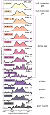 |
Fig. 3. Spectra of fourteen emission lines. We show the spectra of all the emission lines detected within this survey for the central sight line, i.e. aperture of 4″ ≈ 150 pc. The pink dotted rectangle shows the ones we use for discussing line ratio diagnostic plots later in this work (Sect. 6). We normalise all of them to the maximum value in their spectra. The right-hand side indicates what each molecule could be tracing according to literature (we refer the reader to the cautionary statements Sect. 3.2). Within each group we ordered the spectra by their S/N (see Table 3). |
CO is tracing the bulk molecular gas content and its line brightness is up to a factor of 14 higher than other molecular lines within this work (see Table 3). Relative to CO, molecules such as HCN are tracing denser gas, as they get excited at effective densities of n ≳ 103 cm−3. As we go up in neff, HNC, N2H+, CS and HC3N are potentially tracing even denser molecular gas. This means, HC3N is tracing the densest molecular gas in our data set. The spectrum in Fig. 3, however, shows that HC3N has in the central 150 pc the lowest S/N among all our molecular emission lines (S/N of 6). However, as we could see in Table 5, their maximum integrated intensities are located in the SBE, and there we find a S/N of 11 and 36.
Among our molecular species, there are some that reveal more about the chemistry of the gas. The formation path of ethynyl (C2H) is favoured in PDRs by the reaction of C+ with small hydrocarbons and additionally through photodissociation of C2H2 (Meier & Turner 2005, and references therein). This means enhanced C2H in PDRs associated with massive hot cores indicates hidden star formation (Martín et al. 2015; Harada et al. 2018). Recently, Holdship et al. (2021) showed in the nucleus of NGC 253 that high abundances of C2H can be caused by a high cosmic ray ionization rate. We detect C2H(1 − 0) towards the nuclear region of NGC 6946 and the line shows similar to CO and dense gas tracers a broad line profile (FWHM ∼ 200 km s−1) including two peaks.
Strong methanol (CH3OH) emission is considered a tracer of shocks (e.g. Saito et al. 2017). The reason for this is the formation process of CH3OH in the gas phase is not efficient enough to produce higher amounts of CH3OH (Lee et al. 1996). Intense CH3OH emission is believed to arise from a series of hydrogenations of CO on dust grain surfaces under a low-temperature condition (Watanabe et al. 2003). After production on dust, it needs energetic heating mechanisms – shock chemistry – (e.g. Viti et al. 2011; James et al. 2020) to heat the dust and then sublimate CH3OH into the gas phase. However, methanol emission can also be enhanced in non-shocked environments, such as towards massive stars or sources of cosmic ray or X-rays that heat the dust to ∼100 K and allow methanol to evaporate into the gas phase. In our data set, both methanol transitions are stronger in their line brightness than the faintest dense gas tracers – N2H+ and HC3N. Also, both methanol tracers have their maximum integrated intensity peaks in the SBE, where their ratios with CO are higher (ICH3OH/ICO(2 − 1)). Methanol is also known to be a good kinetic temperature probe (e.g. Beuther et al. 2005). Furthermore, para-H2CO transitions can also be used as a temperature indicator which is sensitive to warmer (T > 20 K) and denser (n ∼ 104 − 5 cm−3) gas (e.g. Ginsburg et al. 2016; Mangum et al. 2019). H2CO can be formed in the gas phase as well as on the surface of dust grains (e.g. Terwisscha van Scheltinga et al. 2021). In our data set, H2CO(2 − 1) is one of the faintest lines with S/N ∼ 7 towards the nuclear region.
We note, however, that each molecule is not a unique tracer of a particular process or sets physical conditions in a galaxy. To highlight this point, C2H(1 − 0), for example, in the Milky Way is a tracer of PDRs, yet in NGC 1068 or NGC 253 it is tracing a completely different type of gas (García-Burillo et al. 2017; Holdship et al. 2021). In NGC 1068 it appears to trace a turbulent extended interface between outflows and ISM, yet in NGC 253 it appears to trace the dense gas that is subject to enhanced cosmic-ray ionization rates. Modelling can shed some light on the interpretation, and will be the subject of future work.
Schinnerer et al. (2006) found that the profiles of CO(1−0) and CO(2−1) are double peaked in NGC 6946. In Fig. 3 we also notice double-peaked profiles in the spectra of HCN(1−0), HCO+(1 − 0), HNC(1−0), CS(2−1), CS(3−2), HC3N(10 − 9), N2H+(1−0), C2H(1 − 0), CH3OH(2 − 1) and CH3OH(3 − 2). These could be due to galactic orbital motions or in/outflows in the central 4″ ≈ 150 pc. A more detailed analysis of the kinematics and dynamics of these spectral features are not discussed in this paper but it is planned for a future publication.
In Fig. 3 we denote the peak S/N and what condition each of the molecules can potentially indicate on the right-hand side.
4. The environmental variability of the star formation rate in NGC 6946
We seek answers to how the molecular lines in our data set relate to the current star formation rate (SFR) and if the different environments vary in their SFR on 150 pc scales, or if they have similar characteristics in this respect. We show a map of SFR in panel a of Fig. 4 with contours of tracers of denser gas HCN(1−0) and HNC(1−0), and shock tracer CH3OH(3 − 2) at their native resolution (see Table 2). SFR is peaking at the very centre and drops towards the NBE and SBE.
 |
Fig. 4. Star formation rate map and region mask. Panel a: SFR map with red, orange and green contours of HCN(1−0), HNC(1−0) and CH3OH(3 − 2) integrated intensities (we used the thermal part of the 33 GHz continuum emission at |

To further investigate these differences and the correlations between SFR and the molecular lines in our data set, we convolve the SFR map in units of M⊙ yr−1 to our working resolution of 4″ ≈ 150 pc and sampled it onto a hexagonal grid to match with our integrated intensity maps6. The white contours in panel b of Fig. 4 show the CO(2−1) emission indicating the three distinct features – the nuclear region (NUC) and the northern and southern inner bar ends (NBE and SBE). Since integrated intensities of our dense gas tracers are higher in the SBE than in NBE, we expect to find higher SFR in SBE.
In the following we quote SFR values for the NUC, SBE and NBE which have been averaged over these 150 pc sized regions.
As expected, we find the highest SFR within the NUC, 0.089 M⊙ yr−1. But we see differences in the other two regimes: higher SFR in the SBE than in NBE, 0.013 and 0.006 M⊙ yr−1, respectively7. This agrees with our extended molecular data set, where we find that molecules representing even denser gas, such as N2H+(1−0) or HC3N(10 − 9), reach a maximum in their integrated emission in SBE. Additionally we find the shock tracer CH3OH peaking in their integrated intensities in SBE. This suggests that maybe weak shocks lead to a higher SFR in the SBE compared to the NBE.
The inner bar ends also differ in their molecular masses, as already noted by Schinnerer et al. (2006). We find in our 150 pc sized apertures using Eq. (8) molecular gas mass surface densities (Σmol) of ≈189 ± 0.26 M⊙ pc−2 in the NBE and Σmol ≈ 236 ± 5.09 M⊙ pc−2 in the SBE. We find that the bar ends have a molecular gas depletion time ( ) that is a factor of 10 higher than NUC; the highest in the SBE
  yr (which is rather short, see discussion below).
Towards the NUC we find that stars are formed at a rate of 0.089 M⊙ yr−1 over the past ∼10 Myr8 which translates into 0.89 × 10⁶ M⊙ of recently formed stars. We find Σmol ≈ 298 ± 1.98 M⊙ pc−2 and at the current SFR it will take  years to deplete the present supply of molecular gas. This is shorter (factor of ∼102) than found by previous studies on ∼kpc scales, for example a median Σmol ∼ 2.2 Gyr for the HERACLES galaxies in Leroy et al. (2013), or 1.1 Gyr in Usero et al. (2015). These studies used a Milky Way-like αCO value (a factor of 10 smaller), which is however, not applicable for NGC 6946 (see e.g. Sandstrom et al. 2013; Bigiel et al. 2020 and Sect. 2.3.3). The bar ends have a depletion time of a factor of 10 higher than NUC, and if we calculate
  with a MW value, we would also get into the Gyr range for the bar ends (i.e. ≈1.6 Gyr for NBE and ≈3.3 Gyr for SBE). This demonstrates the importance of adopting a proper αCO factor. The nuclear region of NGC 6946 was studied in terms of its SFR by e.g. Meier & Turner (2004), Schinnerer et al. (2007) and Tsai et al. (2013) using different SFR indicators over different spatial scales.
For example, Schinnerer et al. (2007) found within a 3″ × 3″ square box region a SFR of ∼0.18 M⊙ yr−1 using Paα, 6 cm and 3 mm continuum as SFR tracers9. We find with our 33 GHz based star formation in the same region a SFR of ∼0.11 M⊙ yr−1, that is slightly lower than that of Schinnerer et al. (2007).
We remind the reader that the SFR we calculate is based on free-free emission, which is not subject to the extinction problems that complicate the estimation of SFR at optical and ultraviolet wavelengths. The free-free emission is a tracer of high-mass star formation, as it is only sensitive to stars that are able to ionise the surrounding gas and produce an H II region. However, we have to mention some uncertainties with this SFR. A different choice of initial mass function10, or stellar population models during the calibration of 33 GHz (see Sect. 2.3.2), could introduce a systematic offset in the derived SFR but this should not vary from region to region. The parameter Te in Eq. (4) has an impact of at most ∼7% on the SFR and regional variations in the thermal fraction, fT, are likely to be too small to explain the observed variations in SFR among the bar ends (see e.g. Sect. 4.1 in Querejeta et al. 2019). Another factor that could potentially vary from region to region is the escape fraction of ionising photons (i.e. which part is absorbed in a region outside the 150 pc aperture and therefore does not contribute to the observed free-free emission). However, these uncertainties probably do not explain the factor of 2 higher SFR in the SBE than in the NBE.
5. Results – Line ratios and relationships among molecular species
Molecular line ratios open up the possibility to investigate the physical and chemical state of the ISM. Integrated line ratios among certain molecules were proposed to provide insights into the environment (e.g. HCO+/HCN; Loenen et al. 2008), the temperatures (HCN/HNC; Hacar et al. 2020) and density variations (e.g. line ratio pattern to CO; Leroy et al. 2017). The question can be asked whether we see differences between the inner bar ends and the nuclear region, and if these line ratio diagnostics hold for an extragalactic extreme environment like the centre of NGC 6946. For a meaningful analysis of the line ratios and their relationships, we need to correct the interferometric data for missing short-spacing information. Therefore, we use the five emission lines (CO(1−0), CO(2−1), HCN, HCO+ and HNC) for which single-dish observations were available (see Table 4). The line ratios are calculated from integrated line intensities in units of K km s−1 throughout the entire paper and we refer to them simply as ‘line ratio’.
5.1. Ratios of integrated intensities
In Fig. 5 we show line ratio maps for our SSC + u − v trim data set (see Table 4). We specify the line ratios such that the generally brighter line is in the denominator, while the overall weaker line is in the numerator. The line ratio maps were calculated by only taking integrated intensities with S/N > 5 for the fainter dense gas tracers (DGTs: HCN, HCO+ and HNC) and S/N > 15 for the bulk molecular gas tracers (CO); non-detections were discarded from the line ratio maps:
![Mathematical equation: $$ \begin{aligned} \mathrm{Ratio\,map} = \frac{I_{\rm line_1} \left[I_{\rm line_1}/\sigma _{\rm line_1} > \epsilon \right]}{I_{\rm line_2} \left[I_{\rm line_2}/\sigma _{\rm line_2} > \epsilon \right]}\ {\left\{ \begin{array}{ll} \epsilon = 5&\mathrm{for\,DGTs},\\ \epsilon = 15&\mathrm{for\,CO}. \end{array}\right.} \end{aligned} $$](/articles/aa/full_html/2022/03/aa42624-21/aa42624-21-eq24.gif) (10)
(10)
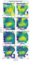 |
Fig. 5. Line ratio maps of the central 20″. We show the line ratio maps for the central 20″ ≈ 750 pc. We overplot on each map contours of the CO(2−1) integrated intensity map in red and denote the features associated with the inner bar (see Fig. 4 for the region mask). |
In the next section, we include non-detections in our analysis. For the case of no significant detection we replaced the values with the upper limits (2σ in Eq. (2)) and include the propagated errors (σprop). We derive them as:
 (11)
(11)
The errors are expressed on a logarithmic scale of base 10 as:
 (12)
(12)
In Fig. 5 the line ratio maps for the central 20″ ≈ 750 pc show differences in line ratios between the environments NUC, SBE and NBE. In the following we report straight mean values over these regions by applying the mask in Fig. 4. The ratios HCO+/HCN and HNC/HCN both show values below unity in all three regions; and over the entire field of view. In both cases, the ratio to HCN is greater in the NUC than in the SBE or NBE.
Looking at the NUC reveals values of 0.81 ± 0.01 and 0.37 ± 0.01 for HCO+/HCN and HNC/HCN, respectively. Ratios to CO indicate higher values in the SBE than in NBE; best visible in the case of HNC/CO(2−1). We discuss the implications of these line ratios in Sects. 6.2–6.4.
5.2. The relationship between molecular lines and SFR surface density
In this section we investigate how our molecular species correlate with ΣSFR and how the dense gas fraction traced by HCN/CO (we investigate also HCO+/CO and HNC/CO) responds to the integrated intensity of CO (an indicator of the mean volume density, see below). We study how these quantities relate to conditions in the centre of NGC 6946. Figure 6 shows the relationships we investigate.
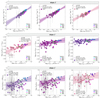 |
Fig. 6. Correlation plots ordered by their slope, β. Dark purple colours show HCN, purple HCO+ and pink HNC. Top row: integrated intensities of the dense gas tracers (ordered by their slope, β) versus ΣSFR. Middle row: integrated intensity of CO(2−1) – an indicator of the mean volume density – versus the line ratio with CO(2−1) – a spectroscopic tracers of fdense. Bottom row: integrated intensity of CO(2−1) – an indicator of the mean volume density – versus the ratio of ΣSFR with the dense gas tracers – a spectroscopic tracers of SFEdense. The linmix fits (accounting for upper limits) are shown as solid lines surrounded by 3σ confidence intervals (shaded regions of corresponding colours). Absolute uncertainties are plotted on each data point, which are generally small towards the regions NUC, NBE and SBE. We find the highest uncertainties in the outskirts in our ΣSFR map. Correlations including HNC result in 58 significant sight lines and 15 upper limits (denoted as light pink markers). We display in each panel Pearson’s correlation coefficient and the power-law slope, intercept and p-value (see Table 6). |
We characterise scaling relations by including upper limits and measurement errors, using the hierarchical Bayesian method described in Kelly (2007). This approach is available as a python package: linmix11. It performs a linear regression of y on x while having measurement errors in both variables and being able to account for non-detections (upper limits) in y. The regression assumes a linear relationship in the form of:
 (13)
(13)
where β is the slope, and α is the y-intercept12. We find Pearson’s correlation coefficients ρ of the data sets for each fitted relationship, and the 3σ confidence intervals are estimated via Markov chain Monte Carlo (MCMC). For a detailed description we refer to Kelly (2007). We provide all the correlations in Table 6.
Scaling relations and correlation coefficients for the central 20″ ≈ 745 pc of NGC 6946 at 150 pc scale.
Dense molecular gas traced by, e.g., HCN emission, has been observed to correlate with SFR (e.g. Gao & Solomon 2004; Lada et al. 2010, 2012). Kauffmann et al. (2017) showed that HCN traces more extended gas and therefore can have an impact on the observed SF trends in galaxies (also see e.g. Pety et al. 2017; Barnes et al. 2020a). Krumholz & Thompson (2007) showed that star formation correlates with any line with a critical density comparable to the median molecular cloud density. Therefore, we expect to see positive correlations between ΣSFR and the surface density of HCN, HCO+ and HNC. In our observations this is confirmed with the additional characteristic that the molecular line with the lowest effective critical density (neff) shows the strongest correlation (neff ordered as HCO+ < HNC < HCN; see Table 2). HCO+ shows the strongest (ρ ∼ 0.95, see Table 6 for uncertainties of ρ) correlation with a slope of β = 1.55 and a small intrinsic scatter:
 (14)
(14)
We note that our slopes are all higher (β > 1) than those found at global scales (β < 1; e.g. Gao & Solomon 2004; Krumholz & Thompson 2007). We speculate that this is due to two contributing factors. Firstly, in this work we are focussing on the centre of NGC 6946 (central 20″ ≈ 745 pc), and not the whole galaxy disc. Hence, this could be due to the limited dynamic range in environmental conditions we are including within the analysis – that is focussing on the densest and most actively star-forming gas within the galaxy. Secondly, this could be a result of the resolution obtained with our PdBI observations. At around 150 pc, we are close to resolving individual discrete star-forming and/or quiescent regions, which could result in the different slope compared to lower resolution studies that include an average on small scale conditions within each sample point; somewhat akin to following a branch of the tuning fork within the recent ‘uncertainty principle for star formation’ framework (Kruijssen et al. 2018, 2019; Chevance et al. 2020a; Kim et al. 2021).
The dense gas fraction, fdense13, usually traced by the integrated intensity of HCN(1−0) over CO, has been observed to increase towards the centres of galaxies (e.g. Usero et al. 2015; Bigiel et al. 2016; Gallagher et al. 2018a; Jiménez-Donaire et al. 2019; Jiang et al. 2020; Bešlić et al. 2021). In turbulent cloud models, increasing the mean volume density of a molecular cloud results in a shift of the gas density distribution to higher densities (e.g. Federrath & Klessen 2013). In addition, the velocity dispersion (or Mach number) widens the density PDF, which causes a larger fraction of the mass to be at higher gas densities. Combined, these increase the fraction of gas above a fixed density (e.g. the effective critical density of HCN), and consequently, these models predict a positive correlation between the volume density and fdense (see Padoan et al. 2014 for a review). Such trends are, in particular, interesting to study within galaxies centres environments thanks to their higher average densities and broader (cloud-scale) line widths compared to typical disc star-forming regions (e.g. Henshaw et al. 2016; Krieger et al. 2020). In the following we use the integrated intensity of CO(2−1) as an indicator of the mean volume density (Leroy et al. 2016; Sun et al. 2018; Gallagher et al. 2018b, see also Sect. 6.4) and explore the dense gas fraction using HCN, HCO+ and HNC. All three fdense versus CO(2−1) fits in Fig. 6 present sub-linear power-law indices (i.e. β < 1.0). We find that the correlations are weakest for the dense gas fraction using HCN (ρ ∼ 0.39) and strongest for HNC/CO(2−1) (ρ ∼ 0.66):
 (15)
(15)
The particular order in the slopes and correlation coefficients do not follow the order of neff as given in Shirley (2015). Instead, they show the order of βHNC > βHCO+ > βHCN (see second row in Fig. 6). Possible explanations for this behaviour could be anomalous excitation for one of the species, for example IR pumping of HCN and HNC levels and/or peculiar filling factors. The star formation efficiency of dense gas (SFEdense) – the ratio of SFR to the integrated intensity of HCN(1−0) – has been observed to decrease towards galaxy centres (same studies as above). This is because the critical overdensity (relative to the mean density) is higher due to the higher Mach number, but also that the absolute critical density (i.e. that obtained from the above line ratios) is higher due to the higher (1) mean density and (2) Mach number (in the context of the CMZ of the Milky Way, see e.g. Kruijssen et al. 2014). Hence, as the mean density of a molecular cloud approaches neff of the molecular line, the line’s intensity will increasingly trace the bulk mass of the cloud, and not exclusively the overdense, star-forming gas; in effect reducing the apparent SFE. From that we would expect to see SFEdense to drop with ICO(2 − 1) (∝volume density) as it has been observed over the disc regions of galaxies (e.g. Gallagher et al. 2018a; Jiménez-Donaire et al. 2019). We use the ratio of ΣSFR to the integrated intensities of the dense gas tracers as SFEdense, and find a different picture of SFEdense with galactocentric radius – increasing towards the NUC; as it shows higher efficiencies in the NUC than in the bar ends (see third row in Fig. 6). We find a moderate14, approximately linear correlation between ΣSFR/IHCN and ICO(2 − 1). The other two SFEdense measurements show weak sub-linear relationships with ρ ∼ 0.46 and ρ ∼ 0.19 for ratios using HCO+ and HNC, respectively. We find that SFEdense increases with increasing ICO(2 − 1), contrary to the trends found by Gallagher et al. (2018a), Jiménez-Donaire et al. (2019). The reason for that could be the special environment of NGC 6946 (inner bar) and/or the different used SFR tracers (we use the free-free emission of 33 GHz continuum compared to Hα + 24 μm and total infrared). Also the above studies could not resolve the inner bar of NGC 6946 (Jiménez-Donaire et al. 2019, angular resolution of 33″ ≈ 1 kpc) or NGC 6946 was not in the nearby disc galaxy sample (Gallagher et al. 2018a). However, we notice, as expected, that stronger correlations in fdense result in weaker correlations in SFEdense and vice versa (e.g. IHNC/ICO(2 − 1) with ρ = 0.76 ± 0.13 and ΣSFR/IHNC with ρ = 0.51 ± 0.24; see Table 6).
6. Implications for spectroscopic studies of other galaxies – from bulk molecular gas to dense gas
Here we discuss some of the common integrated line ratios in more detail and what they can be used for. We compare our high-resolution (150 pc) integrated line ratios of dense gas tracers towards the central region of NGC 6946 with available dense gas tracers from the EMPIRE survey, which include eight additional galaxy centers. It is worth noting that the central regions in the EMPIRE sample are ∼1 kpc sized areas which result in one data point per galaxy (see Jiménez-Donaire et al. 2019 for more details). Nevertheless, it provides us with an understanding of how NGC 6946 compares to other centers.
6.1. R21 variations in the nuclear region and inner bar ends
The CO(2−1)-to-CO(1−0) line ratio, R21, is widely used to convert CO(2−1) emission to CO(1−0), which then can be further converted via the αCO conversion factor to the molecular gas mass. It has been shown that higher R21 values are expected within the central kpc in individual galaxies (Leroy et al. 2009, 2013; Koda et al. 2020). The same trend has been found by den Brok et al. (2021) and Yajima et al. (2021) studying a galaxy sample. NGC 6946 is in both of the aforementioned studies. They find within the central kpc region R21 ∼ 0.7 (at an angular resolution of 33″ ∼ 1 kpc; den Brok et al. 2021 using the EMPIRE sample) and R21 ∼ 1.1 (angular resolution of 17″ ∼ 0.6 kpc; Yajima et al. 2021). However, these studies are not able to resolve variations within the centre between different sub-features. From a physical point of view, R21 should depend on the temperature and density of the gas, as well as on the optical depths of the lines (e.g. Peñaloza et al. 2018). Therefore, understanding how R21 varies in response to the local environment also has the prospect of providing information about the physical conditions of the molecular gas.
With our higher resolution (4″ ≈ 150 pc) observations we are able to resolve smaller-scale structures and thus have the opportunity to investigate variations of R21 within the centre. In Fig. 7 we show R21 against galactocentric radius, highlighting NUC, NBE and SBE in different colours.
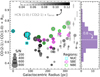 |
Fig. 7. R21 against galactocentric radius. The circular shaped markers represent all of the R21 values for the central 20″ ≈ 745 pc coloured by their fdense. The different sizes show their varying signal-to-noise ratio in CO(2−1). Additionally, we overplot the contours of the three different regions: The cyan colour refers to the nuclear region (NUC), the green to the northern bar end (NBE) and the magenta to the southern bar end (SBE). Along the galactocentric radius, we find in the centre higher R21 values, an initial steady decrease followed by a gradual increase. R21 towards NBE is higher than expected (more in Sect. 6.1). |
We see along the galactocentric radius, in the centre higher R21 values, an initial steady decrease followed by a gradual increase. We find average R21 of 0.65 ± 2E−3 within NUC and even lower values in the southern end of the bar R21 = 0.62 ± 3E−2 (see Table 7). Interestingly, however, we observe higher R21 values towards the northern end of the bar (R21 = 0.70 ± 3E−2) compared to the NUC (factor of ∼1.08), despite the higher ΣSFR in the SBE compared to the NBE (see Sect. 4). The reason for a higher R21 value could be related to denser gas and/or warmer gas with higher temperatures. We colour-code points in Fig. 7 by their HCN(1−0)/CO(2−1) line ratio (∝fdense) and find them showing higher fdense towards the NUC. Furthermore, we would expect to observe higher HCN-to-CO ratios towards the NBE. However, we do not see an increase in the denser gas in the NBE, suggesting a different physical driver for the increased R21 in the NBE. We analyse the three regions regarding their molecular gas density in more detail in Sect. 6.4.
Summary of the characteristics of the nuclear region and inner bar ends of NGC 6946 based on the analyses in this work.
In summary, we find higher R21 values towards one of the inner bar ends of NGC 6946 compared to the nuclear region. If substructures such as small-scale bar ends are to be observed and analysed, R21 may possibly deviate in a minimal way from the kpc-sized R21 values from the literature.
6.2. HNC/HCN: sensitive to kinetic temperatures in extragalactic environments?
In interstellar space, isomers do not necessarily share similar chemical or physical properties. HNC (hydrogen iso-cyanide) and HCN (hydrogen cyanide) isomers are both abundant in cold clouds, but at temperatures exceeding ∼30 K, HNC begins to be converted to HCN by reactions with atomic H. These isomers exhibit an abundance ratio of unity at low temperatures (Schilke et al. 1992; Graninger et al. 2014). A major study to understand this ratio, which was focused on the galactic SF region Orion Molecular Cloud 1 (OMC-1), was carried out by Schilke et al. (1992). They found that the HNC/HCN ratio is ∼1/80 in the direction of Orion Kleinmann-Low (Orion-KL) but increases to 1/5 in regions with lower temperatures near Orion-KL. In the coldest OMC-1 regions, the ratio rises further to 1. The temperature dependence suggests that the ratio must be kinetically controlled (Herbst et al. 2000), so that the integrated intensity line ratio HNC/HCN should decrease at higher temperatures (Pety et al. 2017).
Whether this ratio is sensitive to temperatures in extragalactic sources is uncertain (e.g. Aalto et al. 2002; Meier & Turner 2005, 2012). For example, Meier & Turner (2005) found a kinetic temperature for the centre of IC 342 using the HCN/HNC ratio and the empirical relation of Hirota et al. (1998) of a factor of 2 less than the dust temperature and the kinetic temperature of the gas using CO(2−1) and ammonia (NH3). They suggested that there might be an abundant dense component in IC 342 that is significantly cooler and more uniform than the more diffuse CO, but this was not consistent with the similar distribution of CO, HNC and HCN, unless such a dense component directly follows the diffuse gas. Alternatively, they assumed that this line relationship might not capture temperature, for the nuclear region of IC 342. Also Aalto et al. (2002) find overluminous HNC in many of the most extreme (and presumably warm) (U)LIRGs and suggest that its bright emission cannot be explained by the cool temperatures demanded.
Recently, however, this line ratio has come back into focus. Hacar et al. (2020) demonstrated the strong sensitivity of the HNC/HCN ratio to the gas kinetic temperature, Tk, again towards the Orion star-forming region. They compared the line ratio with NH3 observations (Friesen et al. 2017) and derived Tk from their lower inversion transition ratio NH3 (1, 1)/NH3 (2, 2). In particular, they found that Tk can be described by a two-part linear function for two conditions (we show only Eq. (3) in Hacar et al. 2020):
![Mathematical equation: $$ \begin{aligned} T_{\rm k}\,[\mathrm{K}] = 10 \times \frac{I_{\mathrm{HCN}}}{I_{\mathrm{HNC}}} \quad \mathrm{for} \quad \frac{I_{\mathrm{HCN}}}{I_{\mathrm{HNC}}} \le 4. \end{aligned} $$](/articles/aa/full_html/2022/03/aa42624-21/aa42624-21-eq31.gif) (16)
(16)
However, since the NH3 (1, 1)/NH3 (2, 2) transitions are only sensitive to Tk ≲ 50 K (see e.g. Fig. 1 of Mangum et al. 2013), the calibration shown above only represents the low temperature regime. The challenge of apply such concepts in nearby galaxies is that the concentrations of dense gas studied by Hacar et al. (2020) in the local Milky Way environment (i.e. Orion) are very compact (∼0.1 − 1 pc; Lada & Lada 2003), and representative of solar neighbourhood environmental conditions (e.g. chemistry, and average densities, Mach numbers and kinetic temperatures). Achieving such a resolution is currently extremely difficult in an extragalactic context (e.g. 1 pc = 0.025″ at the distance of the NGC 6946), potentially limiting our capability to determine kinetic temperatures (e.g. when using H2CO; see Mangum et al. 2019 and below). That said, galaxy centres present an ideal regime in which to focus our efforts. As densities similar to the concentrations observed within local star-forming regions are not compact, but can span (nearly) the entire CMZ (so up to 100 pc), leading to luminous and, importantly, extended HCN and HNC emission (Longmore et al. 2013; Rathborne et al. 2015; Krieger et al. 2017; Petkova et al. 2021). Hence, testing this temperature probe within galaxy centres overcomes the requirement for such extremely high-resolution observations, and should be possible with ∼100 pc scale measurements presented in this work.
We find in the nuclear region of NGC 6946 a mean HNC/HCN ratio of ∼0.37. For the bar ends we find lower ratios: ∼0.31 for NBE and ∼0.32 for the SBE (see Table 7). Jiménez-Donaire et al. (2019) reported over kpc-scales a ratio of ∼0.31. There are no other ratios of HNC and HCN in the literature for a comparison, since HNC has hardly been observed towards NGC 6946. If we assume that the ratio of HCN and HNC traces kinetic temperature and adopt the Hacar et al. (2020) relation15, then we would infer a Tk(HCN/HNC) of ∼27 K for the NUC. For the bar ends we calculate slightly higher temperatures of ∼31 K and ∼32 K (on 4″ ≈ 150 pc scales). Meier & Turner (2004) predict Tk ∼ 20 − 40 K (for nH2 = 103 cm−3) based on CO and its isotopologues using a large velocity gradient (LVG) radiative transfer model (building on the models presented in Meier et al. 2000). Including HCN into their LVG models, favoured higher Tk (∼90 K) and nH2 (∼104 − 104.5 cm−3), but these numbers are sensitive to whether 13CO and HCN trace the same gas component. With the inverse transition of NH3, Mangum et al. (2013) found Tk ∼ 47 ± 8 K (using the NH3 (1, 1)/NH3 (2, 2) ratio) which is a factor of ∼2 higher than our inferred Tk (HNC/HCN). The higher excitation NH3 (2, 2)/NH3 (4, 4) ratio, which monitors Tk ≲ 150 K, was not yet detected towards NGC 6946 (Mangum et al. 2013; Gorski et al. 2018). Those studies already showed that an unambiguous determination of the kinetic temperature is challenging.
Comparing our obtained Tk (HNC/HCN) to typical Tk measurements towards the central molecular zone (CMZ) in the Milky Way, reveals higher gas temperatures in the CMZ (Tk > 40 K; Ao et al. 2013; Ott et al. 2014; Ginsburg et al. 2016; Krieger et al. 2017). Investigating individual CMZ clouds, Ginsburg et al. (2016) used para-H2CO transitions as a temperature tracer which is sensitive to warmer (Tk > 20 K) and denser (n ∼ 104 − 5 cm−3) gas. They determined gas temperatures ranging from ∼60 to > 100 K. We know from extragalactic studies that high kinetic temperatures (50 to > 250 K) can be produced by both cosmic ray and mechanical (turbulent) heating processes (Mangum et al. 2013; Gorski et al. 2018). The CMZ of our own Galaxy seems to be different in this respect where the mismatch between dust and gas temperature at moderately high density (n ∼ 104 − 5 cm−3) is better explained by mechanical heating (Ginsburg et al. 2016). However, it is not clear what might be the reason for observing low Tk in an environment where we expect mechanical heating processes.
Compared to the better studied extragalactic nuclear source NGC 253, Mangum et al. (2019) found kinetic temperatures on 5″ ≈ 85 pc scales of Tk > 50 K using ten transitions of H2CO, while on scales < 1″ (∼17 pc) they measure Tk > 300 K. Using NH3 as a thermometer indicates the presence of a warm and hot component with Tk = 75 K and Tk > 150 K, respectively (Gorski et al. 2018; Pérez-Beaupuits et al. 2018). The reported HCN/HNC ratio over the whole nucleus is ∼1, which if Hacar et al. (2020) were true would imply Tk(HNC/HCN)∼10 K. This is in contrast to the aforementioned warm component a factor of 7 lower. It indicates that this ratio provides no reliable information about Tk in the extragalactic region of NGC 253.
We find for the eight kpc-sized galaxy centers in the EMPIRE sample – using Eq. (16) – Tk (HNC/HCN) lower than 50 K for almost all galaxies16. NGC 3627 and NGC 5055 exhibit higher kinetic temperatures, 58 K and 61 K, respectively. Bešlić et al. (2021) found towards NGC 3627 on 100 pc scales (using the same framework) lower Tk (HNC/HCN) of ∼34 K.
In summary, the HNC/HCN ratio results in low inferred kinetic temperatures in galaxy centres (Tk < 50 K) if Hacar et al. (2020) prescription can be applied. However, in the absence of other accurate kinetic temperature measurements (with NH3 or H2CO) against NGC 6946 and the EMPIRE galaxies, we speculate that the isomer ratio is not a suitable Tk probe for large sized extragalactic regions, and, in particular, towards galaxy centres that can also have high optical depths and complex chemistry (also AGN activity and prominent additional excitation mechanisms). A comparison with similarly high resolution observations towards a galaxy centre using kinetic temperatures derived from ammonia emission would be worthwhile to further investigate the HNC/HCN temperature sensitivity framework of Hacar et al. (2020).
6.3. Examining ratios among HCN, HCO+ and HNC as a diagnostic of AGN state
Clouds of gas in the inner kpc of galaxies are exposed to intense radiation, which can emanate from an active galactic nucleus (AGN), seen as hard X-rays with E > 1 keV; from starburst regions, dominated by radiation of O and B stars; or from both. Excess of X-ray emission affects the thermal and chemical balance of the surrounding ISM, which in turn could influence molecular line emission (see below). The centre of NGC 6946 exhibits no clear indication for the presence of an AGN. Holt et al. (2003) studied the distribution of the X-ray emission over the full disc of NGC 6946 and found several low-luminosity point-like sources, one of which coincides with the dynamical centre determined by Schinnerer et al. (2006).
Theoretical modelling of ratios between HCO+ and HCN suggested it as a diagnostic tool to distinguish between photon-dominated regions (PDRs) and X-ray-dominated regions (XDRs) for a given column density of N ∼ 1023 cm−2 in the presence of ionizing radiation (Meijerink & Spaans 2005; Meijerink et al. 2007). In their models the HCO+/HCN ratio seems to systematically vary with gas density, the incident ultraviolet and infrared radiation field. Also mechanical heating and cosmic ray ionization could be possible sources of variations in HCO+/HCN (Bayet et al. 2010; Meijerink et al. 2011). Including HNC to the analyses, Loenen et al. (2008) claims that in XDRs HNC is always stronger than the HCN line, whereas the inverse trend is seen in PDRs (resulting in line ratios lower than unity). For their analyses they used observations obtained with the IRAM 30-m telescope for the HCN, HNC, HCO+ line emission of 37 infrared luminous galaxies (Baan et al. 2008) and additional 80 sources from the literature (see Loenen et al. 2008 and references therein); all unresolved measurements. Then they compared the observational data with the predictions of PDR and XDR models (Meijerink et al. 2007) with varying volume densities, ranging from 104.5 to 106.0 cm−3.
A low HCO+/HCN ratio was proposed as the signature of an AGN. Since studies of galaxies hosting an AGN have found evidence for enhanced emission from HCN, relative to HCO+ (e.g. Kohno et al. 2001; Imanishi et al. 2007; Davies et al. 2012). Recently, however, this statement has been under discussion, for example, in Privon et al. (2020). They investigated NuSTAR hard X-ray emission together with literature HCO+ and HCN observations and found no correlation between the HCO+/HCN ratio and the X-ray to IR luminosity ratio or the AGN luminosity. Thus, observing enhanced HCN relative to HCO+ against a galaxy centre is not convincingly linked to currently observed AGN activity.
We now apply the PDR versus XDR framework by Baan et al. (2008) and Loenen et al. (2008) to our observed dense gas tracers towards the centre of NGC 6946 and investigate Chandra X-ray observations.
We see from the top panels of Fig. 5 that the HCO+/HCN and HNC/HCN ratios exhibit values lower than unity in all three regions (see Table 7). In Fig. 8 we investigate the diagnostic plots proposed by Baan et al. (2008) and Loenen et al. (2008) to visually discriminate between XDR and PDR by comparing the line ratios between HCO+, HCN and HNC in the central 20″ ≈ 745 pc towards NGC 6946. In all these diagnostic plots (panels a–d), NGC 6946 is in the PDR regime. Panel d could indicate a linear relationship between HNC/HCN and HNC/HCO+. We see log10(HNC/HCN) in the range of −0.80 to −0.25 and log10(HNC/HCO+) between −0.70 and +0.10. We investigate which mechanism could cause the observed ranges of line ratios. For this purpose we run the Meijerink & Spaans (2005) models for the PDR case. In particular, we investigate two scenarios: (i) fixing the radiation field (G0 = 102) with varying densities ranging of n = 105 − 106 cm−3, and (ii) fixing the density (n = 105.5 cm−3) with varying radiation field17 of G0 = 102 − 105 (see panel i and ii in Fig. 8). For the first scenario, we find consistent ratios for n ∼ 105.25 − 105.75 cm−3, but the predicted ratios span a narrow range (from log10(HNC/HCO+ = −0.25 to +0.10) compared to the observations (red shaded areas). On the other hand, log10(HNC/HCN) remains rather constant. In the second case, log10(HNC/HCO+) decreases roughly linearly with G0, from −0.2 to −0.7. This corresponds quite well to our observed ranges. From this we conclude that the scatter we observe in log10(HNC/HCO+) (panel d) is mainly due to variations in the radiation field strength, with smaller ratios for stronger radiation fields. From all these diagnostic plots (panels a–d), it seems that the centre of NGC 6946 is dominated by photons (PDR) rather than X-rays (XDR).
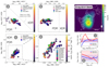 |
Fig. 8. Diagnostic plots using integrated line ratios of HCN, HNC and HCO+ versus each other. Left panels: (a): integrated HCO+/HCN versus HNC/HCO+ ratios. (b): integrated HCO+/HCN versus HNC/HCN ratios. (c): integrated HNC/HCN versus HNC/HCO+ ratios. The grey dashed lines marks the boarder between XDR and PDR (Baan et al. 2008; Loenen et al. 2008). Circles indicate reliable values (S/N > 5) and upper limits for the central 20″ ≈ 745 pc towards NGC 6946. Stars show the EMPIRE galaxies and stars with red contours present galaxy centres hosting an AGN (Goulding & Alexander 2009). For two of them we find ancillary data: the cross shaped markers show the ∼4″ (≈166 pc) M 51 observations (Querejeta et al. 2016) and the ∼2″ (≈100 pc) NGC 3627 observations (Bešlić et al. 2021). (d): the enclosed integrated HNC/HCN versus HNC/HCO+ with the kpc-sized centres of the EMPIRE survey (see Jiménez-Donaire et al. 2019 for details). NGC 6946 and the EMPIRE galaxies are in the PDR regime in all panels. Interestingly, EMPIRE galaxies harbouring an AGN do not show an enhancement of HCN as suggested in many studies (see text for a discussion). We run (Meijerink & Spaans 2005) PDR models for the observed ranges of line ratios (blue and red shaded areas) by (i) fixing the radiation field and (ii) fixing the density. The red and blue lines show the model output (more in text). The colours in (a–d) indicate ΣSFR. We have normalised them to the mean ΣSFR value and find no trend with the integrated line ratios. Upper right panel: X-ray 0.5 − 7.0 keV in counts for NGC 6946 with integrated CO(2−1) contours on top. The black crosses mark the positions of the detected X-ray sources by Holt et al. (2003) which are not strong enough to trigger a XDR. |
For NGC 6946 – as mentioned above – there is no clear evidence for an AGN. In the following we investigate whether there are X-ray sources that are strong enough to trigger an XDR, although the diagnostic diagrams favour a PDR. The Chandra X-ray map (0.5 − 7.0 keV) in counts towards the central 20″ of NGC 6946 shows us that most of the diffuse X-ray emission is coming from a region not associated with the NUC, SBE and NBE (see Fig. 8). The stronger of the two detected X-ray sources near NUC by Holt et al. (2003) (shown as black crosses) is ∼2″ away from the dynamical centre position (shown as red circle). They find a flux of 2.8 × 10⁻¹³ erg s−1 cm−2 and classified its hardness as ‘medium’ (see their Table 2 for SourceID 45). Scaling this flux to our working resolution results in 4.53 × 10⁻³ erg s−1 cm−218. This is similar to the lowest values in Meijerink et al. (2007). This suggests that the brightest X-ray source might affect the gas within a beam scale, but hardly beyond that.
Interestingly, all the kpc-sized central regions of the EMPIRE galaxies in Fig. 8 lie in the PDR regime. Their log10(HNC/HCN) ratios are in the same range as those observed for NGC 6946. On the other hand, log10(HNC/HCO+) varies only from −0.60 to −0.20. The galaxies NGC 3627, NGC 5055 and M 51 are known to host an AGN classified as LINER (Goulding & Alexander 2009) and are still located in the PDR regime in Fig. 8. There is no strong enhanced HCN emission relative to HCO+ towards these three galaxy centres which would ‘move’ them to the XDR regime of the diagnostic plots. The fact that they do not lie within the XDR region of Loenen et al. (2008) could be because: (a) their models are not quantitatively accurate; (b) the EMPIRE AGNs are faint and their effects are diluted when averaging over 1 kpc regions; and (c) a different model that does not require the significant variations in the line ratio to be driven by a PDR or XDR (e.g. Viti 2017). We test the dilution effects in a way that we include available high-resolution dense gas observations of M 51 and NGC 3627 (i.e. ∼4″ ≈ 166 pc from Querejeta et al. 2016 and ∼2″ ≈ 100 pc from Bešlić et al. 2021, respectively; see Sect. 2.3). For both, we show line ratios for the central beam size; they are all in the PDR regime. From that we speculate that the diagnostic plots shown in Fig. 8 and in particular the HCO+/HCN line ratio might not be a unique indicator to diagnose the presence of an AGN in galaxies on kpc/sub-kpc scales. This finding is consistent with the previous studies by Privon et al. (2020) and Li et al. (2021).
6.4. Density variations at the inner bar ends and nuclear region
Already in Fig. 2 we saw that the CO(1−0) and CO(2−1) emission is spatially more extended than HCN(1−0), HCO+(1 − 0) or HNC(1−0), which could be a sign that the CO lines trace a lower density regime. That said, line intensities depend not only on density, but also on optical depth, elemental abundance variations and IR pumping (see e.g. Shirley 2015; Barnes et al. 2020b), and all of these effects can thus drive the relative line intensity ratios.
Leroy et al. (2017) analysed how changes in the sub-beam density distributions affect the beam-averaged line emissivity, by applying non-LTE radiative transfer models coupled with a parametrised density probability distribution. They found that the strength of tracer emission for dense gas is more sensitive to changes in gas density than for example CO. More precisely, the line can still be emitted at densities below the critical density, but with lower efficiency. As a result, a small increase in gas density can significantly increase the efficiency of the emission. This is not the case for lines with a lower critical density (e.g. bulk molecular gas tracer – CO). The density of the gas exceeds the critical density, so varying the gas density does not significantly affect the efficiency of the emission.
We investigate the scenario from Leroy et al. (2017) that line ratios can reflect changes in density distributions. In Fig. 9 we investigate the dependence of the observed molecular line ratios. The colourbar shows the integrated intensity of CO (an indicator of the volume density at cloud scales Leroy et al. 2016; Sun et al. 2018) towards the 150 pc sized NUC, NBE and SBE (see Fig. 4; we take the mean over the 7 hexagonal points). The upper panel shows on the y-axis logarithmic molecular line ratios with CO(2−1). At first glance, within NUC we find line ratios being enhanced by at least 20% compared to the inner bar ends. Identifying ratio variations by eye in the two bar ends is challenging. The lower panel shows the relative differences. Here we divide for example HCN/CO by the mean HCN/CO of all the 3 regions. We ordered them by their flaring appearance. We see the trend is not monotonic with neff, instead they show an order of HCN < HCO+ < HNC; that is the order of decreasing intensity. We find that the highest ratios are associated with NUC (purple marker), except for the CO(1−0)/CO(2−1) ratio. Comparing the two bar ends we find (i) higher ratio values towards the SBE (orange marker) for ratios including CO(1−0) and HCN, (ii) higher ratio values towards the NBE (brown markers) for ratios including HCO+ and HNC and, (iii) that the highest differences between the SBE and NBE is ∼10% which are ratios including CO(1−0) and HCO+. The HCO+ intensity in the SBE seems to be under-luminous compared to the other two environments. The HNC intensity provides the largest dynamic range, with the highest value seen in the NUC and the lowest one in the SBE.
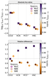 |
Fig. 9. Line ratios for the nuclear region and inner-bar ends. Top: scatter plot showing the mean line ratios of the 7 hexagonal points for each molecule on the y-axis with respect to CO(2−1). For visualisation purpose we spaced the markers along the x-axis. The different shapes of the markers present the defined regions. The colourbar shows the normalised CO(2−1) integrated intensity to the mean CO(2−1) value. We plot the propagated errors in grey and find that they are very small. For the ratios we applied a signal-to-noise cut (see Sect. 5.1). Bottom: the relative differences of the line ratios with respect to the mean of the line ratios among the different regions (linear-scale). |
We compare the observed line ratios of CO, HCN, HCO+ and HNC in the three regions using radiative transfer models to estimate the mass-weighted mean gas density. From the temperature analyses (see Sect. 6.2) we would expect potential higher densities in the bar ends, whereas from the R21 examinations (see Sect. 6.1) we would anticipate higher molecular densities in the NBE than in the SBE. Furthermore, from our derived ΣSFR (see Sect. 4 and Table 7) we would expect higher molecular gas densities in the SBE than in the NBE. For that purpose we use the radiative transfer code Dense Gas Toolbox (Puschnig 2020) which is based on the approach by Leroy et al. (2017) including that emission lines emerge from an isothermal ensemble of gas densities that follow a log-normal distribution (with or without power-law tail) in combination with RADEX calculations (van der Tak et al. 2007). It works as follows: (i) Using Bayesian inference, model parameters (i.e. temperature and density) are inferred from a number of integrated input line intensities. (ii) The assumed fixed line optical depths and abundances are calibrated through observations of the EMPIRE survey (Jiménez-Donaire et al. 2019, which includes NGC 6946). (iii) Then it solves for line emissivities in each density bin which are calculated using expanding-sphere escape probabilities (large velocity gradient approximation) as implemented in RADEX (van der Tak et al. 2007). (iv) Given the estimated kinetic temperature in Sect. 6.2, we are assuming a fixed temperature of 30 K. A more detailed description of the Dense Gas Toolbox will be provided in Puschnig et al. (in prep.). The models suggest that the density in NUC is highest with a mass-weighted mean density of ∼104.0 cm−3, while the lowest one is found in the NBE with a value of ∼103.7 cm−3.
In summary, these models broadly agree with our empirical findings of Fig. 9. The higher mass-weighted mean densities in the SBE agree with the enhanced ΣSFR in the SBE (compared to the NBE). However, the model results do not explain the elevated R21 in NBE (see Fig. 7) and, therefore, an additional physical mechanism has to be responsible for it. A note of caution is appropriate, as the mass-weighted mean density differences found among the three regions are of small magnitude and might not be significant in conjunction with the model assumptions (see Table 7). For example, the kinetic temperature in the model is fixed and the same for the two bar ends and the nuclear region. An accurate measurement of kinetic temperatures on parsec scales could unveil the duality of the bar ends.
7. Conclusion
In this paper we present the high-resolution (2 − 4″ ≈ 75 − 150 pc at 7.7 Mpc distance) IRAM PdBI multi-molecule observation towards the inner 50″ ≈ 1.9 kpc of the Fireworks Galaxy, NGC 6946 (see Fig. 1). Our compiled data set includes a total of 14 detected molecular lines in the mm-wavelength range. For the analyses in this paper, we convolve our molecular lines to a common beam size of 4″, and analyse three distinct environmental regions associated with the inner bar of NGC 6946: the nuclear region (NUC), the northern inner bar end (NBE) and the southern inner bar end (SBE) (see Fig. 4 for mask and Table 7). We find the following results:
-
(1)
We report the first detection of C2H(1 − 0), HC3N(10 − 9) and HC3N(16 − 15) towards NGC 6946.
-
(2)
The different lines show distinct morphology. More extended emission is seen with CO(1−0), CO(2−1) (associated with bulk molecular gas), HCO+(1 − 0), HCN(1−0) and HNC(1−0). The latter three are typically used to trace denser gas. We find that even denser gas (e.g. as seen by N2H+(1−0)) and shocks (e.g. as seen by CH3OH(2 − 1)) are more concentrated in the SBE than in the NUC or NBE (see Fig. 2).
-
(3)
We discover a higher star formation rate (SFR) in the SBE. Shocks and denser gas in this bar end could possibly enhance star formation compared to the lower SFR in NBE.
We use our u − v trimmed and short-spacing corrected data set (SSC + u − v trim data) which includes CO(1−0), CO(2−1), HCN(1−0), HCO+(1 − 0) and HNC(1−0) to investigate how they relate to ΣSFR and how the dense gas fraction (fdense) and the star formation efficiency (SFEdense) respond to the integrated intensity of CO(2−1) (an indicator of mean volume density).
-
(4)
We find among our molecules that HCO+(1 − 0) correlates best with ΣSFR, with Pearson’s correlation coefficient ρ ∼ 0.95. Additionally, we find a relation of ρ to the effective critical density (neff) of the dense gas tracers.
-
(5)
The dense gas fraction fits do not follow the order of neff, instead they show the order of βHNC > βHCO+ > βHCN. The strongest correlation among our mean volume density versus different fdense is ICO(2 − 1) versus HNC/CO(2−1) with ρ ∼ 0.76.
-
(6)
We find that SFEdense increases with increasing gas surface density (i.e. ICO(2 − 1) emission) within the inner ∼1 kpc of NGC 6946, contrary to the opposite trends found within low-resolution observations covering the whole disc (Gallagher et al. 2018a; Jiménez-Donaire et al. 2019). The reason for this is that we are resolving structures within this region, such as the nuclear region (NUC; inner ∼0.15 kpc) that appears to exhibit SFEdense enhancements relative to the rest of the centre.
We test line ratio diagnostic plots and compare our high-resolution (150 pc) dense gas tracer towards NGC 6946 with those of eight other galaxy centres in the EMPIRE survey (angular resolution of 33″ ∼ 1 kpc) and discuss implications for other galaxy centre studies.
-
(7)
From previous studies higher CO(1−0) to CO(2−1) (R21) values are expected in the inner kiloparsec compared to their disc. We find R21 variations in the centre; higher R21 in NBE (∼0.7) than in the NUC or SBE (∼0.65 and ∼0.62). The reason for this could be, for example, denser gas that is in the NBE. However, we do not find an increase of higher fdense in NBE (see Fig. 7 and Table 7).
-
(8)
Whether the ratio between HCN and HNC is temperature dependent has been discussed by several authors in the past. We speculate that the isomer ratio is not an accurate probe for kinetic temperatures for kiloparsec and sub-kiloparsec sized extragalactic regions. This is because, if the prescription of Hacar et al. (2020) can be applied here, the HCN/HNC ratio results in low Tk (< 50 K, for NGC 6946 as well as for six EMPIRE galaxies, IC 342 and NGC 253) which is up to a factor of 7 lower compared to other existing Tk measurements (NH3 or H2CO).
-
(9)
The observed HCO+/HCN ratios have been proposed to be a diagnostic tool to distinguish between XDR and PDR. The diagnostic plots for the centre of NGC 6946 favour a PDR. We find that an X-ray source about 2″ away from the dynamical centre does not affect the molecular gas properties in the nucleus. However, when we include the EMPIRE galaxy centres in our analysis, we find that those galaxies that have an active galactic nucleus (AGN) fall within the PDR range in these diagnostic diagrams. We find for two of these AGN host galaxies higher resolution observations (∼100 pc for NGC 3627 and ∼166 pc for M 51) which also lay in the PDR regime. Thus, the HCO+/HCN ratio might not be a unique indicator to diagnose AGN activity in galaxies at (sub-)kiloparsec scales. This ambiguity is consistent with recent studies (see Fig. 8 and Sect. 6.3).
-
(10)
Molecular line ratios may reflect changes in the (unresolved) gas density distributions (Leroy et al. 2017). The ratios to CO, show enhanced line ratios within the NUC compared to the inner bar ends. HCO+(1 − 0) in NBE seems to be under-luminous compared to the NUC and SBE. On the other hand, HNC provides the largest dynamic range, with the highest values in the NUC and the lowest in the SBE (see Fig. 9). We compared that with radiative transfer models and find mass-weight mean densities of ∼103.7 − 4.3 cm−3 for the NUC, while the NBE shows the lowest mean density of ∼103.3 − 4.1 cm−3. The higher mean densities in the SBE compared to the NBE agree with the higher integrated line intensities and the enhanced SFR in the SBE.
This study reflects the importance of analysing molecular lines to better understand galactic centres. Also, it shows that bar ends in galaxies can vary in their dense gas fraction, star formation rate, integrated line ratios and molecular gas densities. In future work we follow up on the investigation of shocks, the densest gas tracers in our extended data set and examine the kinematic and dynamic of the inner bar in more detail.
The majority of the discussed studies throughout this work, observed the base transitions of molecules such as HCN and HCO+, which become excited at effective critical densities of n > 3 × 103 cm−3 (e.g. Shirley 2015). This is then typically referred to in the literature as ‘dense gas’, relative to the density of gas traced by CO (n ≈ 102 cm−3).
We note that the 3 mm emission lines of C2H, N2H+, and HC3N were covered by EMPIRE, but not included in the public release.
The effective critical densities, neff, are defined in Table 2.
We do this also with our ΣSFR map in units of M⊙ yr−1 kpc−2 to calculate star formation efficiencies of the dense molecular gas (see Eq. (8)).
We calculate the uncertainties for these SFR values using the uncertainty 33 GHz map and apply the equations as in Sect. 2.3.2. We then get over a 4″ region a SFR uncertainty of ±1.35 × 10⁻³ M⊙ yr−1.
Recall that the approximate age sensitivity of the thermal fraction of the 33 GHz continuum emission as a SFR tracer is ∼10 Myr.
They adopted a distance of 5.5 Mpc to NGC 6946 for their SFR calculations. We have re-scaled their value to the distance of 7.7 Mpc using a factor of 1.8, see Appendix A.1.
As well as any potential stochasticity due to IMF sampling.
We specify the covariance between the measurement errors in x and y (xycov parameter) and set K = 2.
In this work, we take the CO(2−1) data for our fdense estimates because they have a higher S/N and better quality than CO(1−0).
Here we refer to a moderate correlation if ρ lies in the range of 0.5 − 0.7.
The equation in Hacar et al. (2020) uses HCN over HNC (HCN/HNC), therefore we have for e.g. NUC = 1/0.37 = 2.7.
For NGC 3627, NGC 4254 and NGC 5055 we had to take for the calibration the second part of the two-part linear function in Hacar et al. (2020).
G0 = 102 and G0 = 105 are the default minimum and maximum G0 in their model outputs.
Assuming the source is point-like, we scale the flux by (D/d)2, where D is the distance to NGC 6946 and d is the distance from the X-ray source, 2″.
Acknowledgments
We would like to thank the anonymous referee for their insightful comments that helped improve the quality of the paper. C.E. gratefully acknowledges funding from the Deutsche Forschungsgemeinschaft (DFG) Sachbeihilfe, grant number BI1546/3-1. F.B., A.B., I.B., J.P. and J.d.B. acknowledge funding from the European Research Council (ERC) under the European Union’s Horizon 2020 research and innovation programme (grant agreement No. 726384/Empire). E.S., D.L., H.A.P., T.S. and T.G.W. acknowledge funding from the European Research Council (ERC) under the European Union’s Horizon 2020 research and innovation programme (grant agreement No. 694343). I.L. acknowledges funding from the Deutsche Forschungsgemeinschaft (DFG) Sachbeihilfe, grant number SCHI 536/11-1. M.C. and J.M.D.K. gratefully acknowledge funding from the Deutsche Forschungsgemeinschaft (DFG) in the form of an Emmy Noether Research Group (grant number KR4801/1-1) and the DFG Sachbeihilfe (grant number KR4801/2-1), and from the European Research Council (ERC) under the European Union’s Horizon 2020 research and innovation programme via the ERC Starting Grant MUSTANG (grant agreement number 714907). H.H. acknowledges the support of the Natural Sciences and Engineering Research Council of Canada (NSERC), funding reference number RGPIN-2017-03987 and the Canadian Space Agency funding reference 21EXPUVI3. SCOG and RSK acknowledge financial support from the German Research Foundation (DFG) via the collaborative research center (SFB 881, Project-ID 138713538) ‘The Milky Way System’ (subprojects A1, B1, B2, and B8). They also acknowledge funding from the Heidelberg Cluster of Excellence ‘STRUCTURES’ in the framework of Germany’s Excellence Strategy (grant EXC-2181/1, Project-ID 390900948) and from the European Research Council via the ERC Synergy Grant ‘ECOGAL’ (grant 855130). The work of AKL is partially supported by the National Science Foundation under Grants No. 1615105, 1615109, and 1653300. J.P. acknowledges support from the Programme National “Physique et Chimie du Milieu Interstellaire” (PCMI) of CNRS/INSU with INC/INP co-funded by CEA and CNES. M.Q. acknowledges support from the Spanish grant PID2019-106027GA-C44, funded by MCIN/AEI/10.13039/501100011033. E.R. acknowledges the support of the Natural Sciences and Engineering Research Council of Canada (NSERC), funding reference number RGPIN-2017-03987. T.S. acknowledges funding from the European Research Council (ERC) under the European Union’s Horizon 2020 research and innovation programme (grant agreement No. 694343). M.C.S. acknowledges financial support from the German Research Foundation (DFG) via the collaborative research center (SFB 881, Project-ID 138713538) “The Milky Way System” (subprojects A1, B1, B2, and B8). A.U. acknowledges support from the Spanish grants PGC2018-094671-B-I00, funded by MCIN/AEI/10.13039/501100011033 and by “ERDF A way of making Europe”, and PID2019-108765GB-I00, funded by MCIN/AEI/10.13039/501100011033. Y.-H.T. acknowledges funding support from NRAO Student Observing Support Grant SOSPADA-012 and from the National Science Foundation (NSF) under grant No. 2108081. Y.G. acknowledges support by National Key Basic R&D Program of China (2017YFA0402704), NSFC grants 11861131007 and 12033004.
References
- Aalto, S., Polatidis, A. G., Hüttemeister, S., & Curran, S. J. 2002, A&A, 381, 783 [NASA ADS] [CrossRef] [EDP Sciences] [Google Scholar]
- Aladro, R., Viti, S., Bayet, E., et al. 2013, A&A, 549, A39 [NASA ADS] [CrossRef] [EDP Sciences] [Google Scholar]
- Anand, G. S., Rizzi, L., & Tully, R. B. 2018, AJ, 156, 105 [NASA ADS] [CrossRef] [Google Scholar]
- Ao, Y., Henkel, C., Menten, K. M., et al. 2013, A&A, 550, A135 [NASA ADS] [CrossRef] [EDP Sciences] [Google Scholar]
- Astropy Collaboration (Robitaille, T. P., et al.) 2013, A&A, 558, A33 [NASA ADS] [CrossRef] [EDP Sciences] [Google Scholar]
- Astropy Collaboration (Price-Whelan, A. M., et al.) 2018, AJ, 156, 123 [Google Scholar]
- Baan, W. A., Henkel, C., Loenen, A. F., Baudry, A., & Wiklind, T. 2008, A&A, 477, 747 [NASA ADS] [CrossRef] [EDP Sciences] [Google Scholar]
- Barnes, A. T., Longmore, S. N., Battersby, C., et al. 2017, MNRAS, 469, 2263 [Google Scholar]
- Barnes, A. T., Longmore, S. N., Avison, A., et al. 2019, MNRAS, 486, 283 [NASA ADS] [CrossRef] [Google Scholar]
- Barnes, A. T., Longmore, S. N., Dale, J. E., et al. 2020a, MNRAS, 498, 4906 [NASA ADS] [CrossRef] [Google Scholar]
- Barnes, A. T., Kauffmann, J., Bigiel, F., et al. 2020b, MNRAS, 497, 1972 [NASA ADS] [CrossRef] [Google Scholar]
- Bayet, E., Awad, Z., & Viti, S. 2010, ApJ, 725, 214 [NASA ADS] [CrossRef] [Google Scholar]
- Belloche, A., Müller, H. S. P., Menten, K. M., Schilke, P., & Comito, C. 2013, A&A, 559, A47 [NASA ADS] [CrossRef] [EDP Sciences] [Google Scholar]
- Bemis, A., & Wilson, C. D. 2019, AJ, 157, 131 [NASA ADS] [CrossRef] [Google Scholar]
- Beuther, H., Thorwirth, S., Zhang, Q., et al. 2005, ApJ, 627, 834 [CrossRef] [Google Scholar]
- Beuther, H., Meidt, S., Schinnerer, E., Paladino, R., & Leroy, A. 2017, A&A, 597, A85 [NASA ADS] [CrossRef] [EDP Sciences] [Google Scholar]
- Bešlić, I., Barnes, A. T., Bigiel, F., et al. 2021, MNRAS, 506, 963 [CrossRef] [Google Scholar]
- Bigiel, F., Leroy, A. K., Blitz, L., et al. 2015, ApJ, 815, 103 [NASA ADS] [CrossRef] [Google Scholar]
- Bigiel, F., Leroy, A. K., Jiménez-Donaire, M. J., et al. 2016, ApJ, 822, L26 [NASA ADS] [CrossRef] [Google Scholar]
- Bigiel, F., de Looze, I., Krabbe, A., et al. 2020, ApJ, 903, 30 [CrossRef] [Google Scholar]
- Billington, S. J., Urquhart, J. S., König, C., et al. 2020, MNRAS, 499, 2744 [Google Scholar]
- Bolatto, A. D., Wolfire, M., & Leroy, A. K. 2013, ARA&A, 51, 207 [CrossRef] [Google Scholar]
- Callanan, D., Longmore, S. N., Kruijssen, J. M. D., et al. 2021, MNRAS, 505, 4310 [NASA ADS] [CrossRef] [Google Scholar]
- Chevance, M., Kruijssen, J. M. D., Hygate, A. P. S., et al. 2020a, MNRAS, 493, 2872 [NASA ADS] [CrossRef] [Google Scholar]
- Chevance, M., Kruijssen, J. M. D., Vazquez-Semadeni, E., et al. 2020b, Space Sci. Rev., 216, 50 [NASA ADS] [CrossRef] [Google Scholar]
- Combes, F., García-Burillo, S., Casasola, V., et al. 2013, A&A, 558, A124 [NASA ADS] [CrossRef] [EDP Sciences] [Google Scholar]
- Cormier, D., Bigiel, F., Jiménez-Donaire, M. J., et al. 2018, MNRAS, 475, 3909 [NASA ADS] [CrossRef] [Google Scholar]
- Crosthwaite, L. P. 2002, PASP, 114, 929 [NASA ADS] [CrossRef] [Google Scholar]
- Davies, R., Mark, D., & Sternberg, A. 2012, A&A, 537, A133 [NASA ADS] [CrossRef] [EDP Sciences] [Google Scholar]
- de Blok, W. J. G., Walter, F., Brinks, E., et al. 2008, AJ, 136, 2648 [NASA ADS] [CrossRef] [Google Scholar]
- de Lorenzo-Cáceres, A., Méndez-Abreu, J., Thorne, B., & Costantin, L. 2020, MNRAS, 494, 1826 [Google Scholar]
- den Brok, J. S., Chatzigiannakis, D., Bigiel, F., et al. 2021, MNRAS, 504, 3221 [NASA ADS] [CrossRef] [Google Scholar]
- de Vaucouleurs, G., de Vaucouleurs, A., Corwin, H. G., Jr., et al. 1991, Third Reference Catalogue of Bright Galaxies (New York: Springer) [Google Scholar]
- Díaz-García, S., Moyano, F. D., Comerón, S., et al. 2020, A&A, 644, A38 [NASA ADS] [CrossRef] [EDP Sciences] [Google Scholar]
- Dickinson, C., Ali-Haïmoud, Y., Barr, A., et al. 2018, New Astron. Rev., 80, 1 [CrossRef] [Google Scholar]
- Elmegreen, D. M., Chromey, F. R., & Santos, M. 1998, AJ, 116, 1221 [NASA ADS] [CrossRef] [Google Scholar]
- Emsellem, E., Goudfrooij, P., & Ferruit, P. 2003, MNRAS, 345, 1297 [NASA ADS] [CrossRef] [Google Scholar]
- Emsellem, E., Renaud, F., Bournaud, F., et al. 2015, MNRAS, 446, 2468 [Google Scholar]
- Engelbracht, C. W., Rieke, M. J., Rieke, G. H., & Latter, W. B. 1996, ApJ, 467, 227 [NASA ADS] [CrossRef] [Google Scholar]
- Erwin, P. 2011, Mem. Soc. Astron. It. Suppl., 18, 145 [Google Scholar]
- Federrath, C., & Klessen, R. S. 2013, ApJ, 763, 51 [Google Scholar]
- Font, J., Beckman, J. E., Zaragoza-Cardiel, J., et al. 2014, MNRAS, 444, L85 [NASA ADS] [CrossRef] [Google Scholar]
- Friesen, R. K., Pineda, J. E., Rosolowsky, E., et al. 2017, ApJ, 843, 63 [NASA ADS] [CrossRef] [Google Scholar]
- Gallagher, M. J., Leroy, A. K., Bigiel, F., et al. 2018a, ApJ, 858, 90 [NASA ADS] [CrossRef] [Google Scholar]
- Gallagher, M. J., Leroy, A. K., Bigiel, F., et al. 2018b, ApJ, 868, L38 [CrossRef] [Google Scholar]
- Gao, Y., & Solomon, P. M. 2004, ApJS, 152, 63 [Google Scholar]
- García-Burillo, S., Viti, S., Combes, F., et al. 2017, A&A, 608, A56 [Google Scholar]
- Ginsburg, A., Henkel, C., Ao, Y., et al. 2016, A&A, 586, A50 [NASA ADS] [CrossRef] [EDP Sciences] [Google Scholar]
- Gorski, M., Ott, J., Rand, R., et al. 2018, ApJ, 856, 134 [NASA ADS] [CrossRef] [Google Scholar]
- Goulding, A. D., & Alexander, D. M. 2009, MNRAS, 398, 1165 [NASA ADS] [CrossRef] [Google Scholar]
- Graninger, D. M., Herbst, E., Öberg, K. I., & Vasyunin, A. I. 2014, ApJ, 787, 74 [Google Scholar]
- Hacar, A., Bosman, A. D., & van Dishoeck, E. F. 2020, A&A, 635, A4 [NASA ADS] [CrossRef] [EDP Sciences] [Google Scholar]
- Harada, N., Sakamoto, K., Martín, S., et al. 2018, ApJ, 855, 49 [Google Scholar]
- Helfer, T. T., & Blitz, L. 1993, ApJ, 419, 86 [NASA ADS] [CrossRef] [Google Scholar]
- Henkel, C., Mühle, S., Bendo, G., et al. 2018, A&A, 615, A155 [NASA ADS] [CrossRef] [EDP Sciences] [Google Scholar]
- Henshaw, J. D., Longmore, S. N., Kruijssen, J. M. D., et al. 2016, MNRAS, 457, 2675 [Google Scholar]
- Herbst, E., Terzieva, R., & Talbi, D. 2000, MNRAS, 311, 869 [NASA ADS] [CrossRef] [Google Scholar]
- Hirota, T., Yamamoto, S., Mikami, H., & Ohishi, M. 1998, ApJ, 503, 717 [Google Scholar]
- Holdship, J., Viti, S., Martín, S., et al. 2021, A&A, 654, A55 [NASA ADS] [CrossRef] [EDP Sciences] [Google Scholar]
- Holt, S. S., Schlegel, E. M., Hwang, U., & Petre, R. 2003, ApJ, 588, 792 [NASA ADS] [CrossRef] [Google Scholar]
- Imanishi, M., Nakanishi, K., Tamura, Y., Oi, N., & Kohno, K. 2007, AJ, 134, 2366 [NASA ADS] [CrossRef] [Google Scholar]
- James, T. A., Viti, S., Holdship, J., & Jiménez-Serra, I. 2020, A&A, 634, A17 [EDP Sciences] [Google Scholar]
- Jiang, X.-J., Greve, T. R., Gao, Y., et al. 2020, MNRAS, 494, 1276 [NASA ADS] [CrossRef] [Google Scholar]
- Jiménez-Donaire, M. J., Bigiel, F., Leroy, A. K., et al. 2019, ApJ, 880, 127 [CrossRef] [Google Scholar]
- Kauffmann, J., Goldsmith, P. F., Melnick, G., et al. 2017, A&A, 605, L5 [NASA ADS] [CrossRef] [EDP Sciences] [Google Scholar]
- Kelly, B. C. 2007, ApJ, 665, 1489 [Google Scholar]
- Kelly, G., Viti, S., Bayet, E., Aladro, R., & Yates, J. 2015, A&A, 578, A70 [NASA ADS] [CrossRef] [EDP Sciences] [Google Scholar]
- Kennicutt, R. C., & Evans, N. J. 2012, ARA&A, 50, 531 [NASA ADS] [CrossRef] [Google Scholar]
- Kennicutt, R. C., Jr., Armus, L., Bendo, G., et al. 2003, PASP, 115, 928 [NASA ADS] [CrossRef] [Google Scholar]
- Kennicutt, R. C., Calzetti, D., Aniano, G., et al. 2011, PASP, 123, 1347 [Google Scholar]
- Kessler, S., Leroy, A., Querejeta, M., et al. 2020, ApJ, 892, 23 [NASA ADS] [CrossRef] [Google Scholar]
- Kim, J., Chevance, M., Kruijssen, J. M. D., et al. 2021, MNRAS, 504, 487 [NASA ADS] [CrossRef] [Google Scholar]
- Klessen, R. S., & Glover, S. C. O. 2016, Saas-Fee Advanced Course, 43, 85 [Google Scholar]
- Koda, J., Sawada, T., Sakamoto, K., et al. 2020, ApJ, 890, L10 [NASA ADS] [CrossRef] [Google Scholar]
- Kohno, K., Matsushita, S., Vila-Vilaró, B., et al. 2001, in The Central Kiloparsec of Starbursts and AGN: The La Palma Connection, eds. J. H. Knapen, J. E. Beckman, I. Shlosman, & T. J. Mahoney, ASP Conf. Ser., 249, 672 [NASA ADS] [Google Scholar]
- Krieger, N., Ott, J., Beuther, H., et al. 2017, ApJ, 850, 77 [NASA ADS] [CrossRef] [Google Scholar]
- Krieger, N., Bolatto, A. D., Leroy, A. K., et al. 2020, ApJ, 897, 176 [Google Scholar]
- Kroupa, P. 2001, MNRAS, 322, 231 [NASA ADS] [CrossRef] [Google Scholar]
- Kruijssen, J. M. D., Longmore, S. N., Elmegreen, B. G., et al. 2014, MNRAS, 440, 3370 [Google Scholar]
- Kruijssen, J. M. D., Schruba, A., Hygate, A. P. S., et al. 2018, MNRAS, 479, 1866 [NASA ADS] [CrossRef] [Google Scholar]
- Kruijssen, J. M. D., Schruba, A., Chevance, M., et al. 2019, Nature, 569, 519 [NASA ADS] [CrossRef] [Google Scholar]
- Krumholz, M. R., & Thompson, T. A. 2007, ApJ, 669, 289 [NASA ADS] [CrossRef] [Google Scholar]
- Krumholz, M. R., Kruijssen, J. M. D., & Crocker, R. M. 2017, MNRAS, 466, 1213 [Google Scholar]
- Lada, C. J., & Lada, E. A. 2003, ARA&A, 41, 57 [Google Scholar]
- Lada, C. J., Lombardi, M., & Alves, J. F. 2010, ApJ, 724, 687 [Google Scholar]
- Lada, C. J., Forbrich, J., Lombardi, M., & Alves, J. F. 2012, ApJ, 745, 190 [NASA ADS] [CrossRef] [Google Scholar]
- Lee, H. H., Bettens, R. P. A., & Herbst, E. 1996, A&AS, 119, 111 [NASA ADS] [CrossRef] [EDP Sciences] [Google Scholar]
- Leitherer, C., Schaerer, D., Goldader, J. D., et al. 1999, ApJS, 123, 3 [Google Scholar]
- Leroy, A. K., Walter, F., Bigiel, F., et al. 2009, AJ, 137, 4670 [Google Scholar]
- Leroy, A. K., Walter, F., Sandstrom, K., et al. 2013, AJ, 146, 19 [Google Scholar]
- Leroy, A. K., Hughes, A., Schruba, A., et al. 2016, ApJ, 831, 16 [Google Scholar]
- Leroy, A. K., Usero, A., Schruba, A., et al. 2017, ApJ, 835, 217 [NASA ADS] [CrossRef] [Google Scholar]
- Leroy, A. K., Bolatto, A. D., Ostriker, E. C., et al. 2018, ApJ, 869, 126 [NASA ADS] [CrossRef] [Google Scholar]
- Leroy, A. K., Hughes, A., Liu, D., et al. 2021, ApJS, 255, 19 [NASA ADS] [CrossRef] [Google Scholar]
- Levine, E. S., Helfer, T. T., Meijerink, R., & Blitz, L. 2008, ApJ, 673, 183 [NASA ADS] [CrossRef] [Google Scholar]
- Li, F., Wang, J., Gao, F., et al. 2021, MNRAS, 503, 4508 [NASA ADS] [CrossRef] [Google Scholar]
- Linden, S. T., Murphy, E. J., Dong, D., et al. 2020, ApJS, 248, 25 [NASA ADS] [CrossRef] [Google Scholar]
- Loenen, A. F., Spaans, M., Baan, W. A., & Meijerink, R. 2008, A&A, 488, L5 [NASA ADS] [CrossRef] [EDP Sciences] [Google Scholar]
- Long, K. S., Winkler, P. F., & Blair, W. P. 2019, ApJ, 875, 85 [NASA ADS] [CrossRef] [Google Scholar]
- Longmore, S. N., Bally, J., Testi, L., et al. 2013, MNRAS, 429, 987 [NASA ADS] [CrossRef] [Google Scholar]
- Mangum, J. G., Darling, J., Henkel, C., et al. 2013, ApJ, 779, 33 [CrossRef] [Google Scholar]
- Mangum, J. G., Ginsburg, A. G., Henkel, C., et al. 2019, ApJ, 871, 170 [NASA ADS] [CrossRef] [Google Scholar]
- Martín, S., Kohno, K., Izumi, T., et al. 2015, A&A, 573, A116 [NASA ADS] [CrossRef] [EDP Sciences] [Google Scholar]
- Mauersberger, R., & Henkel, C. 1989, IAU Circ., 4889, 1 [NASA ADS] [Google Scholar]
- Mauersberger, R., & Henkel, C. 1991, A&A, 245, 457 [NASA ADS] [Google Scholar]
- Mauersberger, R., Henkel, C., Wilson, T. L., & Harju, J. 1989, A&A, 226, L5 [NASA ADS] [Google Scholar]
- McKee, C. F., & Ostriker, E. C. 2007, ARA&A, 45, 565 [Google Scholar]
- Meier, D. S., & Turner, J. L. 2004, AJ, 127, 2069 [CrossRef] [Google Scholar]
- Meier, D. S., & Turner, J. L. 2005, ApJ, 618, 259 [NASA ADS] [CrossRef] [Google Scholar]
- Meier, D. S., & Turner, J. L. 2012, ApJ, 755, 104 [NASA ADS] [CrossRef] [Google Scholar]
- Meier, D. S., Turner, J. L., & Hurt, R. L. 2000, ApJ, 531, 200 [CrossRef] [Google Scholar]
- Meier, D. S., Walter, F., Bolatto, A. D., et al. 2015, ApJ, 801, 63 [NASA ADS] [CrossRef] [Google Scholar]
- Meijerink, R., & Spaans, M. 2005, A&A, 436, 397 [CrossRef] [EDP Sciences] [Google Scholar]
- Meijerink, R., Spaans, M., & Israel, F. P. 2007, A&A, 461, 793 [NASA ADS] [CrossRef] [EDP Sciences] [Google Scholar]
- Meijerink, R., Spaans, M., Loenen, A. F., & van der Werf, P. P. 2011, A&A, 525, A119 [NASA ADS] [CrossRef] [EDP Sciences] [Google Scholar]
- Méndez-Abreu, J., de Lorenzo-Cáceres, A., Gadotti, D. A., et al. 2019, MNRAS, 482, L118 [Google Scholar]
- Menéndez-Delmestre, K., Sheth, K., Schinnerer, E., Jarrett, T. H., & Scoville, N. Z. 2007, ApJ, 657, 790 [Google Scholar]
- Morris, M., & Serabyn, E. 1996, ARA&A, 34, 645 [Google Scholar]
- Murphy, E. J., Condon, J. J., Schinnerer, E., et al. 2011, ApJ, 737, 67 [Google Scholar]
- Murphy, E. J., Bremseth, J., Mason, B. S., et al. 2012, ApJ, 761, 97 [Google Scholar]
- Murphy, E. J., Dong, D., Leroy, A. K., et al. 2015, ApJ, 813, 118 [NASA ADS] [CrossRef] [Google Scholar]
- Murphy, E. J., Dong, D., Momjian, E., et al. 2018, ApJS, 234, 24 [NASA ADS] [CrossRef] [Google Scholar]
- Nguyen, Q. R., Jackson, J. M., Henkel, C., Truong, B., & Mauersberger, R. 1992, ApJ, 399, 521 [NASA ADS] [CrossRef] [Google Scholar]
- Ott, J., Weiß, A., Staveley-Smith, L., Henkel, C., & Meier, D. S. 2014, ApJ, 785, 55 [NASA ADS] [CrossRef] [Google Scholar]
- Padoan, P., Federrath, C., Chabrier, G., et al. 2014, in Protostars and Planets VI, eds. H. Beuther, R. S. Klessen, C. P. Dullemond, & T. Henning, 77 [Google Scholar]
- Palagi, F., Cesaroni, R., Comoretto, G., Felli, M., & Natale, V. 1993, A&AS, 101, 153 [Google Scholar]
- Pan, H.-A., Kuno, N., Koda, J., et al. 2015, ApJ, 815, 59 [NASA ADS] [CrossRef] [Google Scholar]
- Peñaloza, C. H., Clark, P. C., Glover, S. C. O., & Klessen, R. S. 2018, MNRAS, 475, 1508 [CrossRef] [Google Scholar]
- Pérez-Beaupuits, J. P., Güsten, R., Harris, A., et al. 2018, ApJ, 860, 23 [Google Scholar]
- Petkova, M. A., Kruijssen, J. M. D., Kluge, A. L., et al. 2021, MNRAS, submitted [arXiv:2104.09558] [Google Scholar]
- Pety, J., Schinnerer, E., Leroy, A. K., et al. 2013, ApJ, 779, 43 [NASA ADS] [CrossRef] [Google Scholar]
- Pety, J., Guzmán, V. V., Orkisz, J. H., et al. 2017, A&A, 599, A98 [NASA ADS] [CrossRef] [EDP Sciences] [Google Scholar]
- Privon, G. C., Ricci, C., Aalto, S., et al. 2020, ApJ, 893, 149 [NASA ADS] [CrossRef] [Google Scholar]
- Puschnig, J. 2020, https://doi.org/10.5281/zenodo.3686329 [Google Scholar]
- Querejeta, M., Schinnerer, E., García-Burillo, S., et al. 2016, A&A, 593, A118 [NASA ADS] [CrossRef] [EDP Sciences] [Google Scholar]
- Querejeta, M., Schinnerer, E., Schruba, A., et al. 2019, A&A, 625, A19 [NASA ADS] [CrossRef] [EDP Sciences] [Google Scholar]
- Rathborne, J. M., Longmore, S. N., Jackson, J. M., et al. 2015, ApJ, 802, 125 [Google Scholar]
- Regan, M. W., & Vogel, S. N. 1995, ApJ, 452, L21 [NASA ADS] [Google Scholar]
- Renaud, F., Bournaud, F., Emsellem, E., et al. 2015, MNRAS, 454, 3299 [NASA ADS] [CrossRef] [Google Scholar]
- Rodriguez-Fernandez, N., Pety, J., & Gueth, F. 2008, Single-dish Observation and Processing to Produce the Short-spacing Information for a Millimeter Interferometer, IRAM Memo 2008-2 [Google Scholar]
- Rosolowsky, E., & Leroy, A. 2006, PASP, 118, 590 [NASA ADS] [CrossRef] [Google Scholar]
- Rosolowsky, E., Hughes, A., Leroy, A. K., et al. 2021, MNRAS, 502, 1218 [NASA ADS] [CrossRef] [Google Scholar]
- Saito, T., Iono, D., Espada, D., et al. 2017, ApJ, 834, 6 [Google Scholar]
- Salak, D., Tomiyasu, Y., Nakai, N., et al. 2018, ApJ, 856, 97 [CrossRef] [Google Scholar]
- Sandstrom, K. M., Leroy, A. K., Walter, F., et al. 2013, ApJ, 777, 5 [Google Scholar]
- Schilke, P., Walmsley, C. M., Pineau Des Forets, G., et al. 1992, A&A, 256, 595 [Google Scholar]
- Schinnerer, E., Böker, T., Emsellem, E., & Lisenfeld, U. 2006, ApJ, 649, 181 [NASA ADS] [CrossRef] [Google Scholar]
- Schinnerer, E., Böker, T., Emsellem, E., & Downes, D. 2007, A&A, 462, L27 [NASA ADS] [CrossRef] [EDP Sciences] [Google Scholar]
- Shirley, Y. L. 2015, PASP, 127, 299 [Google Scholar]
- Solomon, P. M., Downes, D., & Radford, S. J. E. 1992, ApJ, 387, L55 [NASA ADS] [CrossRef] [Google Scholar]
- Sormani, M. C., & Barnes, A. T. 2019, MNRAS, 484, 1213 [NASA ADS] [CrossRef] [Google Scholar]
- Sormani, M. C., Tress, R. G., Glover, S. C. O., et al. 2020, MNRAS, 497, 5024 [Google Scholar]
- Sun, J., Leroy, A. K., Schruba, A., et al. 2018, ApJ, 860, 172 [NASA ADS] [CrossRef] [Google Scholar]
- Tan, Q.-H., Gao, Y., Zhang, Z.-Y., et al. 2018, ApJ, 860, 165 [NASA ADS] [CrossRef] [Google Scholar]
- Terwisscha van Scheltinga, J., Hogerheijde, M. R., Cleeves, L. I., et al. 2021, ApJ, 906, 111 [Google Scholar]
- Tsai, C.-W., Turner, J. L., Beck, S. C., Meier, D. S., & Wright, S. A. 2013, ApJ, 776, 70 [NASA ADS] [CrossRef] [Google Scholar]
- Usero, A., Leroy, A. K., Walter, F., et al. 2015, AJ, 150, 115 [Google Scholar]
- van der Tak, F. F. S., Black, J. H., Schöier, F. L., Jansen, D. J., & van Dishoeck, E. F. 2007, A&A, 468, 627 [NASA ADS] [CrossRef] [EDP Sciences] [Google Scholar]
- Viti, S. 2017, A&A, 607, A118 [NASA ADS] [CrossRef] [EDP Sciences] [Google Scholar]
- Viti, S., Jimenez-Serra, I., Yates, J. A., et al. 2011, ApJ, 740, L3 [NASA ADS] [CrossRef] [Google Scholar]
- Walter, F., Brinks, E., de Blok, W. J. G., et al. 2008, AJ, 136, 2563 [Google Scholar]
- Watanabe, N., Shiraki, T., & Kouchi, A. 2003, ApJ, 588, L121 [Google Scholar]
- Yajima, Y., Sorai, K., Miyamoto, Y., et al. 2021, PASJ, 73, 257 [NASA ADS] [CrossRef] [Google Scholar]
Appendix A: Star formation rates
In this work, we used the 33 GHz continuum emission as a SFR tracer. We also found published 15 GHz and Hα observations in comparable angular resolution of our molecular data set (2″; see Table A.1). We chose the 33 GHz over the 15 GHz as a SFR tracer because the 33 GHz observations are: (1) higher in sensitivity (9.72 compared to 21.44 mK, Linden et al. 2020), and (2) probe less non-thermal emission (38% compared to 63%, see Equations below). We did not use extinction corrected Hα data (from Kessler et al. 2020) for our main SFR in this paper because: (1) they used 2″ sized apertures across the whole galaxy covering the bright Hα emitting regions (1σ threshold in Hα) for the extinction correction (using Paβ) and those apertures do not fully cover the inner kpc of NGC 6946, and (2) causes them to miss a handful of heavily attenuated regions in the centre of NGC 6946 (see Fig. 2 in Kessler et al. 2020).
In the following we check the consistency of our SFR derived from the 33 GHz thermal part of the radio continuum emission with the thermal part of the 15 GHz as a ΣSFR tracer (observations from Murphy et al. 2018; Linden et al. 2020) for the inner kpc-sized region of NGC 6946.
-
33 GHz continuum: Using 33 GHz for the inner 1 kpc gives us a mean ΣSFR of 0.792 M⊙ yr−1 kpc−2.
-
15 GHz continuum: Before we can use Eq. (4), we first have to compute the thermal fraction (fT) at 15 GHz. We recall that we denote thermal as T, non-thermal as NT and the frequency as ν. Knowing that
 with αT ∼ 0.1 and
  with αNT ∼ 0.74 (from Murphy et al. 2011 for the nucleus of NGC 6946), we find:
 (A.1)
(A.1)We take as in Section 2.3.2
 and find using Eq. (A.1) that
  . Now we are able to calculate LνT (Eq. (5)) and use Eq. (4) to convert the thermal fluxes into a SFR and further to ΣSFR. Within the central kpc-sized region we get a mean ΣSFR of 0.774 M⊙ yr−1 kpc−2.
We conclude, that the ΣSFR for the inner kpc derived from 33 GHz and 15 GHz are within the margin of error (∼1σ).
A.1. Correcting for distance
Schinnerer et al. (2007) found within a 3″ × 3″ region a SFR of ∼0.1 M⊙ yr−1 adopting a distance of 5.5 Mpc. Using 33 GHz as a SFR tracer and taking the same distance and region, we get 0.06 M⊙ yr−1. Adopting the updated distance to NGC 6946 of 7.72 Mpc results in 0.11 M⊙ yr−1. This is only a factor of 1.8 higher.
References of the data shown in Fig. 1.
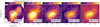 |
Fig. A.1. SSC + uv trim integrated intensity maps: The way of presenting the data is done as in Figure 2. Here, however, we performed a u − v cut and corrected for the short-spacing using available EMPIRE data for the three typical dense gas tracers. In the first two panels we show contours of 200, 300σ and in the remaining three panels contours of 3, 6, 9, 30, 60, 90σ. |
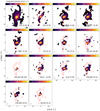 |
Fig. A.2. Same as Figure 2 but only showing hexagonal points with S/N > 25 for CO(1−0) and CO(2−1), and with S/N > 5 for all other lines. |
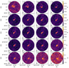 |
Fig. A.3. HCN channel maps, from −80 to 110 km s−1. |
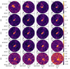 |
Fig. A.4. HCO+ channel maps, from −80 to 110 km s−1. |
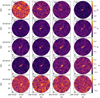 |
Fig. A.5. HNC channel maps, from -80 to 110 km s−1. |
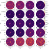 |
Fig. A.6. CS(2-1) channel maps, from -80 to 110 km s−1. |
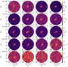 |
Fig. A.7. CS(3-2) channel maps, from -80 to 110 km s−1. |
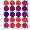 |
Fig. A.8. N2H+ channel maps, from -80 to 110 km s−1. |
 |
Fig. A.9. CH3OH(2k-1k) channel maps, from -80 to 110 km s−1. |
 |
Fig. A.10. CH3OH(3k-2k) channel maps, from -80 to 110 km s−1. |
 |
Fig. A.11. C2H(1-0) channel maps, from -80 to 110 km s−1. |
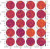 |
Fig. A.12. HC3N(10-9) channel maps, from -80 to 110 km s−1. |
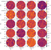 |
Fig. A.13. HC3N(16-15) channel maps, from -80 to 110 km s−1. |
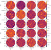 |
Fig. A.14. H2CO(2-1) channel maps, from -80 to 110 km s−1. |
All Tables
Summary of the molecular lines in our compiled data set towards the centre of NGC 6946.
Scaling relations and correlation coefficients for the central 20″ ≈ 745 pc of NGC 6946 at 150 pc scale.
Summary of the characteristics of the nuclear region and inner bar ends of NGC 6946 based on the analyses in this work.
All Figures
|
Fig. 1. Gallery of the multi-wavelength observation towards the centre of NGC 6946. Left panels: (a) three colour optical image, with the region of interest drawn as a purple box, (b) CO(1−0) emission shown in contours levels of 60, 90, 200, 300, 600 K km−1 s−1, and are repeated on all panels for comparison, (c) integrated CO(1−0) emission, (d) CO(2−1) emission towards the inner 20″ shown as colour scale; sketch (right): denoting all observed features (see Sect. 2.4 for an overview), (e)–(g) continuum emission, (h)–(j) infrared emission and (k)–(m) hydrogen recombination lines and X-ray emission (see Table A.1 for references of all observations shown). The rightmost column shows integrated intensity maps of three of our fourteen detected emission lines for comparison. Optical image credits: NASA, ESA, STScI, R. Gendler, and the Subaru Telescope (NAOJ). |
| In the text | |
|
Fig. 2. Integrated intensity maps (moment 0) for 14 molecular emission lines at a common resolution of 4″ ≈ 150 pc. The maps were created using a hexagonal sampling with half a beam spacing, where CO(1−0) was used as a mask. The grey shaded circle in the lower left corner marks the beam size and the red contours show CO(1−0) S/N levels of 30, 60 and 90. The white contours in the first panel show S/N levels of 200 and 300, and in the second panel S/N levels of 30, 60 and 90. The following panels (from HCN to H2CO(2 − 1)) show S/N levels of 3, 6, 9, 30, 60 and 90. The colourbar indicates the integrated intensity of each line in units of K km s−1. See Table 1 for the properties of this data set. |
| In the text | |
|
Fig. 3. Spectra of fourteen emission lines. We show the spectra of all the emission lines detected within this survey for the central sight line, i.e. aperture of 4″ ≈ 150 pc. The pink dotted rectangle shows the ones we use for discussing line ratio diagnostic plots later in this work (Sect. 6). We normalise all of them to the maximum value in their spectra. The right-hand side indicates what each molecule could be tracing according to literature (we refer the reader to the cautionary statements Sect. 3.2). Within each group we ordered the spectra by their S/N (see Table 3). |
| In the text | |
|
Fig. 4. Star formation rate map and region mask. Panel a: SFR map with red, orange and green contours of HCN(1−0), HNC(1−0) and CH3OH(3 − 2) integrated intensities (we used the thermal part of the 33 GHz continuum emission at |
| In the text | |
|
Fig. 5. Line ratio maps of the central 20″. We show the line ratio maps for the central 20″ ≈ 750 pc. We overplot on each map contours of the CO(2−1) integrated intensity map in red and denote the features associated with the inner bar (see Fig. 4 for the region mask). |
| In the text | |
|
Fig. 6. Correlation plots ordered by their slope, β. Dark purple colours show HCN, purple HCO+ and pink HNC. Top row: integrated intensities of the dense gas tracers (ordered by their slope, β) versus ΣSFR. Middle row: integrated intensity of CO(2−1) – an indicator of the mean volume density – versus the line ratio with CO(2−1) – a spectroscopic tracers of fdense. Bottom row: integrated intensity of CO(2−1) – an indicator of the mean volume density – versus the ratio of ΣSFR with the dense gas tracers – a spectroscopic tracers of SFEdense. The linmix fits (accounting for upper limits) are shown as solid lines surrounded by 3σ confidence intervals (shaded regions of corresponding colours). Absolute uncertainties are plotted on each data point, which are generally small towards the regions NUC, NBE and SBE. We find the highest uncertainties in the outskirts in our ΣSFR map. Correlations including HNC result in 58 significant sight lines and 15 upper limits (denoted as light pink markers). We display in each panel Pearson’s correlation coefficient and the power-law slope, intercept and p-value (see Table 6). |
| In the text | |
|
Fig. 7. R21 against galactocentric radius. The circular shaped markers represent all of the R21 values for the central 20″ ≈ 745 pc coloured by their fdense. The different sizes show their varying signal-to-noise ratio in CO(2−1). Additionally, we overplot the contours of the three different regions: The cyan colour refers to the nuclear region (NUC), the green to the northern bar end (NBE) and the magenta to the southern bar end (SBE). Along the galactocentric radius, we find in the centre higher R21 values, an initial steady decrease followed by a gradual increase. R21 towards NBE is higher than expected (more in Sect. 6.1). |
| In the text | |
|
Fig. 8. Diagnostic plots using integrated line ratios of HCN, HNC and HCO+ versus each other. Left panels: (a): integrated HCO+/HCN versus HNC/HCO+ ratios. (b): integrated HCO+/HCN versus HNC/HCN ratios. (c): integrated HNC/HCN versus HNC/HCO+ ratios. The grey dashed lines marks the boarder between XDR and PDR (Baan et al. 2008; Loenen et al. 2008). Circles indicate reliable values (S/N > 5) and upper limits for the central 20″ ≈ 745 pc towards NGC 6946. Stars show the EMPIRE galaxies and stars with red contours present galaxy centres hosting an AGN (Goulding & Alexander 2009). For two of them we find ancillary data: the cross shaped markers show the ∼4″ (≈166 pc) M 51 observations (Querejeta et al. 2016) and the ∼2″ (≈100 pc) NGC 3627 observations (Bešlić et al. 2021). (d): the enclosed integrated HNC/HCN versus HNC/HCO+ with the kpc-sized centres of the EMPIRE survey (see Jiménez-Donaire et al. 2019 for details). NGC 6946 and the EMPIRE galaxies are in the PDR regime in all panels. Interestingly, EMPIRE galaxies harbouring an AGN do not show an enhancement of HCN as suggested in many studies (see text for a discussion). We run (Meijerink & Spaans 2005) PDR models for the observed ranges of line ratios (blue and red shaded areas) by (i) fixing the radiation field and (ii) fixing the density. The red and blue lines show the model output (more in text). The colours in (a–d) indicate ΣSFR. We have normalised them to the mean ΣSFR value and find no trend with the integrated line ratios. Upper right panel: X-ray 0.5 − 7.0 keV in counts for NGC 6946 with integrated CO(2−1) contours on top. The black crosses mark the positions of the detected X-ray sources by Holt et al. (2003) which are not strong enough to trigger a XDR. |
| In the text | |
|
Fig. 9. Line ratios for the nuclear region and inner-bar ends. Top: scatter plot showing the mean line ratios of the 7 hexagonal points for each molecule on the y-axis with respect to CO(2−1). For visualisation purpose we spaced the markers along the x-axis. The different shapes of the markers present the defined regions. The colourbar shows the normalised CO(2−1) integrated intensity to the mean CO(2−1) value. We plot the propagated errors in grey and find that they are very small. For the ratios we applied a signal-to-noise cut (see Sect. 5.1). Bottom: the relative differences of the line ratios with respect to the mean of the line ratios among the different regions (linear-scale). |
| In the text | |
|
Fig. A.1. SSC + uv trim integrated intensity maps: The way of presenting the data is done as in Figure 2. Here, however, we performed a u − v cut and corrected for the short-spacing using available EMPIRE data for the three typical dense gas tracers. In the first two panels we show contours of 200, 300σ and in the remaining three panels contours of 3, 6, 9, 30, 60, 90σ. |
| In the text | |
|
Fig. A.2. Same as Figure 2 but only showing hexagonal points with S/N > 25 for CO(1−0) and CO(2−1), and with S/N > 5 for all other lines. |
| In the text | |
|
Fig. A.3. HCN channel maps, from −80 to 110 km s−1. |
| In the text | |
|
Fig. A.4. HCO+ channel maps, from −80 to 110 km s−1. |
| In the text | |
|
Fig. A.5. HNC channel maps, from -80 to 110 km s−1. |
| In the text | |
|
Fig. A.6. CS(2-1) channel maps, from -80 to 110 km s−1. |
| In the text | |
|
Fig. A.7. CS(3-2) channel maps, from -80 to 110 km s−1. |
| In the text | |
|
Fig. A.8. N2H+ channel maps, from -80 to 110 km s−1. |
| In the text | |
|
Fig. A.9. CH3OH(2k-1k) channel maps, from -80 to 110 km s−1. |
| In the text | |
|
Fig. A.10. CH3OH(3k-2k) channel maps, from -80 to 110 km s−1. |
| In the text | |
|
Fig. A.11. C2H(1-0) channel maps, from -80 to 110 km s−1. |
| In the text | |
|
Fig. A.12. HC3N(10-9) channel maps, from -80 to 110 km s−1. |
| In the text | |
|
Fig. A.13. HC3N(16-15) channel maps, from -80 to 110 km s−1. |
| In the text | |
|
Fig. A.14. H2CO(2-1) channel maps, from -80 to 110 km s−1. |
| In the text | |
Current usage metrics show cumulative count of Article Views (full-text article views including HTML views, PDF and ePub downloads, according to the available data) and Abstracts Views on Vision4Press platform.
Data correspond to usage on the plateform after 2015. The current usage metrics is available 48-96 hours after online publication and is updated daily on week days.
Initial download of the metrics may take a while.